

Submitted:
30 April 2026
Posted:
01 May 2026
You are already at the latest version
Abstract
Smart microgrids combining photovoltaic arrays, wind turbines, and battery storage generate telemetry that existing open-source monitoring tools cannot process with per-mechanism energy loss visibility in real time. This paper presents a design, im-plementation, and evaluation of an open-source IoT Monitoring Framework. The framework incorporates a physics-based microgrid simulator, a hierarchical MQTT communication architecture, and a React-based web-based user interface that supports WebSocket-based real-time data visualization. The open-source framework consists of twelve containerized microservices that can be started with a single command: docker compose up -d. The code has been released under the permissive MIT license. All stack performance testing was conducted using a simulated 1 hour test case based on a 100kWp PV system, 10kW wind turbine, and 50kWh battery powered campus mi-crogrid. Average P50 end-to-end latency was 27.2 ms and P99 end-to-end latency was 48.3 ms with 100% message delivery across 5,840 test messages with per-topic analy-sis revealing a 25 ms serialization-order effect in sequential MQTT publishing. Com-parative analysis against ten existing platforms including OpenEMS, VOLTTRON, Eclipse Ditto, and pymgrid confirms that no prior open-source framework unifies physics-based loss telemetry, IoT communication, time-series storage, and real-time visualization in a single reproducible deployment.
Keywords:
digital twin
; smart microgrid
; MQTT
; IoT
; real-time monitoring
; energy losses
; open-source
; physics-based simulation
1. Introduction
Since 2020, the deployment of distributed photovoltaic systems in Europe has grown by more than 40% annually [10], driving campus-scale and community microgrids into configurations that conventional SCADA systems were never designed to monitor. A microgrid combining PV arrays, small wind turbines, battery storage, and time-varying building loads generates heterogeneous telemetry, power flows, voltages, frequencies, state of charge, and weather conditions at sub-minute intervals. Tracking these measurements in real time is a solved problem for a single metering point. Tracking them across a dozen assets while simultaneously determining where energy is lost between the panel and the common connection point, contamination, cable resistance, inverter conversion, transformer core magnetization doesn't happen. That is the monitoring gap this paper addresses.
Digital twin technology has emerged as a candidate solution. A digital twin, in the energy context, is a virtual replica of a physical system synchronized through IoT communication, enabling monitoring, simulation, and decision support without interrupting the physical asset [1,3]. Digital twin for microgrids have attracted considerable attention in recent years. Although, there are six review papers and articles written between 2024 and 2025 on digital twin applications for smart grids and renewable energy systems [1,3,4,5,6], and two other have addressed specific topologies of microgrids [2,7]. Despite the numerous surveys on the topic, the field is very poor in terms of actual, deployable implementations. Out of 112 papers on digital twins for smart energy published by Aghazadeh Ardebili et al. [5] in , 107 of them are based on the conceptual design of digital twins or simulation results without any runnable code, IoT communication layers, or a step-by-step guide for their real-world deployments.
Current solutions only cover fragments of the required capabilities. OpenEMS [29] provides energy flow calculations in a Java OSGi bundle structure and thus serves as a good base. However, it lacks an MQTT communication layer and also a physics-based loss model. VOLTTRON [31], provided by Pacific Northwest National Laboratory, is an agent-based architecture that provides a communication framework using its own protocol. However, it is focused on building-connected applications and not for microgrid-related use cases. Eclipse Ditto [32] is a generic solution for digital twins and is well-engineered. It supports MQTT messaging and comes with a REST API to manage the state of a digital twin. But, comes without energy equations, microgrid-specific topic hierarchies and without a dashboard. ThingsBoard [33] is an open-source software for data collection from IoT devices using MQTT protocol, and creation of configurable interactive web dashboards. However, the community edition is limited in aspect of connected devices, and there is no physics simulation engine built-in. For microgrid simulation using reinforcement learning, we found pymgrid [11], a Python open-source software library for research simulation of microgrid. While it has capabilities for microgrid simulation, it outputs arrays of numerical values and lacks functions for deployment and real-time monitoring of time-series data from various IoT devices and sensors. Another relevant numerical calculation library is pvlib [12] which computes PV energy losses with high fidelity using validated models including the CEC inverter curves [15] and NOCT cell temperature estimates, but it is a calculation library, not a monitoring platform. For example, Hamid et al. [14] built a MATLAB-based digital twin of a large PV plant with high accuracy (prediction accuracy of 99.77%) in a controlled environment, while it is proprietary framework that cannot be freely distributed or even containerized. Sivaneasan et al. [2] came closest, their Cognitive DT for a Singapore microgrid achieved 0.24% cost deviation in a real-world deployment, but it uses proprietary components, focuses on optimization rather than monitoring, and does not publish itemized loss telemetry. Izquierdo Monge et al. [28] built an open-source monitoring and alarm system for microgrids, but it lacks physics-based loss models and does not report MQTT performance benchmarks. And the most recent MQTT performance study for microgrid communication Kondoro et al. [8] is now five years old and tested simpler payloads on different hardware.
In our previous work [30], we presented a web-based hybrid optimization platform for real-time microgrid energy management at SoftCOM 2025. That system demonstrated the viability of combining genetic algorithm and reinforcement learning optimizers with LSTM-based load forecasting for battery dispatch scheduling. But it was built on Flask (synchronous), had no IoT communication layer, no physics-based loss models, and no containerized deployment, precisely the limitations that motivated the present study.
The gaps in existing approaches fall into four distinct categories: (a) reliance on proprietary tools that prevent reproducibility, (b) absence of physics-based energy loss models that quantify where generation is lost between source and load, (c) lack of real-time IoT communication layers with structured topic hierarchies and published latency analysis, and (d) no reproducible performance benchmarks against which alternative implementations can be compared. In light of these gaps, this paper makes the following four contributions:
1. An end-to-end open-source digital twin architecture comprising twelve Docker services: simulator, MQTT broker, data-ingestion subscriber, API gateway, time-series database, in-memory cache, frontend dashboard, reverse proxy, and four supporting services deployable via a single `docker compose up -d` command under the MIT license.
2. A physics-based microgrid simulator implementing nine distinct energy loss mechanisms applied sequentially at 5-second resolution: PV soiling (Kimber linear model [16]), module mismatch, DC cable I²R losses, CEC inverter efficiency curves [15], AC distribution cable losses, transformer iron-copper losses, battery self-discharge, BMS parasitic draw, and wind mechanical losses, each published as itemized MQTT telemetry per simulation step.
3. A hierarchical MQTT topic architecture with QoS 1 at-least-once delivery, six topic patterns carrying per-asset measurements including full loss breakdowns, and a dual-write ingestion pipeline that routes messages simultaneously to TimescaleDB hypertables for historical storage and to Valkey pub/sub channels for sub-second WebSocket delivery to the dashboard.
4. Reproducible performance benchmarks from a one-hour automated test demonstrating P50 end-to-end latency of 27.2 ms, P99 of 48.3 ms, 100% message delivery reliability across 5,840 messages, and a per-topic latency analysis revealing the serialization-order effect inherent in sequential MQTT publishing, the first such benchmark for a microgrid digital twin framework since Kondoro et al. [8] in 2021.
The remainder of this paper is organized as follows. Section 2 describes the system architecture, simulator, MQTT, data pipeline, web interface and deployment. Section 3 presents the experimental results like latency, throughput, reliability, loss model validation, and platform comparison. In section 4 we discuss key findings, Industry 5.0 alignment, and limitations. Section 5 concludes with specific future research directions.
2. Materials and Methods
This section covers the overall architecture of the framework, the detailed simulation model using a physics-based simulator, loss models, MQTT communication, data ingestion, real-time visualisation, and a containerized deployment. The code for all components is open-source and can be deployed on a single machine with a single Docker Compose command
2.1. System Architecture Overview
Twelve containerized services. That is the full count not a monolithic application partitioned after the fact, but twelve independent services, each with its own failure domain, each designed and implemented from the ground up to serve a specific purpose and with no shared runtime state.
The architecture used for building the campus microgrid digital twin is shown in Figure 1. The architecture is four-layered, progressing from simulation down to application. The Simulation Layer consists of a physics-based microgrid simulator that models PV generation, wind power, campus loads, battery storage and nine energy loss mechanisms within the microgrid. The simulator models each at a 5-second time step. The IoT Transport Layer includes the IoT broker - Eclipse Mosquitto MQTT message broker [25] - and the data-ingestion service used to subscribe to all telemetry topics on the broker and route them to storage and real-time microservices as required. The Data Layer consists of TimescaleDB [22] - a PostgreSQL 16 extension that automatically partitions data into hypertables - supplemented by a Valkey open-source Redis-compatible cache that is used to cache the digital twin state and provide a WebSocket pub/sub bridge between simulation, data store and application layers. The Application Layer consists of a FastAPI [23] REST and WebSocket gateway that serves up a React 18 web-based dashboard to the end-user, as well as Traefik-based HTTP routing.
In addition to the main data path through the bot, we also have two supporting layers that get hit from time to time. To monitor load and performance, Prometheus is configured to scrape the /metrics endpoint from each of the four backends every 15 seconds, which gets rendered out into a bunch of Grafana dashboards. We also have a bunch of forecasting and optimization services (PyTorch LSTM and DEAP genetic algorithm, respectively) that talk to the TimescaleDB database and Valkey cache, but those are not exercised in this paper, they form the subject of our next publication, which builds on the monitoring infrastructure described here.
In the table below you can find the entire stack of technology used. Every part of the stack consists of open-source components with license that suit our needs: all of them have permissive free-to-use licenses (open-source MIT license, Apache-2.0, EPL-2.0, BSD-3). We choose TimescaleDB instead of InfluxDB for our time-series database for support of full SQL and ability to utilize the many PostgreSQL features and tools like pg_dump, psql, and Alembic for schema migrations. For the cache we picked Valkey over Redis after the relicensing of Redis in 2024, an event that created ambiguity in the license. We utilize Zustand [24] for our dashboard state store because we only want to have to write as much boilerplate as necessary. We chose Mosquitto [25] because it uses very little memory and proven reliability in IoT deployments.

Table 1.
Technology stack of the proposed framework.
| Layer | Technology | Version | License | Role |
|---|---|---|---|---|
| Simulator | Python 3.12 | 3.12+ | PSF | Physics engine |
| MQTT Broker | Eclipse Mosquitto | 2.0+ | EPL-2.0 | Message transport |
| Backend | FastAPI | 0.115+ | MIT | REST API + WebSocket |
| Time-Series DB | TimescaleDB (PG 16) | 2.17+ | Apache-2.0 | Measurement storage |
| Cache / Broker | Valkey | 8.0+ | BSD-3 | Pub/sub + state cache |
| Frontend | React 18 + TypeScript | 18.3+ | MIT | Dashboard UI |
| UI Components | shadcn/ui + Radix | latest | MIT | Accessible primitives |
| Charts | Recharts | 2.12+ | MIT | Data visualization |
| State Management | Zustand | 5+ | MIT | Client state |
| Containerization | Docker Compose | 27+ | Apache-2.0 | Orchestration |
| Monitoring | Prometheus + Grafana | latest | Apache / AGPL | Metrics + alerting |
| Reverse Proxy | Traefik | 3.2+ | MIT | Routing + TLS |
2.2. Physics-Based Microgrid Simulator
The simulator is the "physics engine" of the digital twin. It reads weather data from either a recorded CSV profile or synthetic AR(1) stochastic weather generation, and then computes the electrical state of every asset at each time step. Also, simulator fetches real-time weather from the Open-Meteo API [34] (Lipjan, Kosovo coordinates) when running at 1x speed. The electrical state of every asset is then computed, applying loss models sequentially, and the results are then published out as a set of structured MQTT messages.
2.2.1. Simulation Pipeline Overview
This results in the long pipeline illustrated in Figure 2 for each simulation timestep. The first four steps of this process compute the basic generation and demand: raw weather (irradiance, temperature, wind speed, humidity, rain indicator), raw generation from equation (1), raw wind generation from a cubic power curve defined by cut-in, rated, and cut-out (3 m/s, 12 m/s, 25 m/s for the 10 kW turbine), and campus building load from an interpolated diurnal load profile that ranges from a 30 kW nighttime base load to an 80 kW daytime peak load.
In Step 5 of the loss chain, the 9 mechanisms for loss are applied in sequence to compute the lossy transformation from gross generation to net power delivered. Following that, Steps 6 through 8 handle demand-response curtailment, diesel, and EV charging, which are enabled/disabled based on configuration. Step 9 applies a time-of-use aware battery dispatch strategy. Step 10 calculates the SoC of batteries including self discharge and BMS parasitic current drain according to Equation (7). Step 11 calculates the grid power balance at the PCC per Equation (8). Finally, Step 12 publishes results via MQTT with detailed breakdown of losses. You can configure the simulation speed, from 1× (real time) up to 3,600× (one hour simulated per real second), or even faster if needed. At 3,600× speed, with a 5-second physics interval, the simulator can produce an average of 720 steps per simulated hour, and approximately 8 MQTT messages per step, spread across 7 different topic types.
2.2.2. Photovoltaic Model with Energy Loss Chain
PV model starts with DC output of PV system equation:
where G is plane-of-array irradiance (W/m²), A = 555 m² is total panel area, η₀ = 0.18 is reference efficiency at standard test conditions, and β = 0.004 K⁻¹ is the temperature power coefficient. Cell temperature is estimated via the NOCT model:
with NOCT = 45 °C. At 30 °C ambient and 800 W/m² irradiance, cell temperature reaches 55 °C, causing approximately 12% power derating.
Table 2.
Energy loss model parameters.
| # | Loss Mechanism | Model | Default Value | Configurable |
|---|---|---|---|---|
| 1 | PV Soiling | Kimber linear + rain reset [16] | 0.2%/day | Yes |
| 2 | PV Mismatch | Fixed factor | 1.5% | Yes |
| 3 | DC Cable | I^2R at 600 V | R = 0.15 Ω | Yes |
| 4 | PV Inverter | CEC weighted [15] | 100 kW SMA ref. | Yes |
| 5 | AC Cable | I^2R at 400 V, 3-phase | R = 0.08 Ω | Yes |
| 6 | Transformer | Iron + copper | 250 kVA, 0.75 + 3 kW | Yes |
| 7 | Battery Self-Discharge | Linear SOC drain | 2%/month | Yes |
| 8 | BMS Parasitic | Constant draw | 50 W | Yes |
| 9 | Wind Mechanical | Drivetrain + yaw | 5% + 2% | Yes |
Nine loss mechanisms are then applied in sequence. Figure 3 shows the loss chain from gross DC to net AC delivery and the table 2 lists all parameters.
Soiling follows the Kimber linear accumulation model [16]:
where r_soil = 0.002 per day is the daily accumulation rate and d_rain(t) is days since last rainfall. A rain event resets the soiling factor to 0.95 (not 1.0, residual dust persists). After 25 consecutive dry days, the factor saturates at its floor of 0.85.
Module mismatch is modeled as a fixed 1.5% derating factor, representing manufacturing variance and thermal non-uniformity across the string.
DC cable losses follow an ohmic I²R model:
with R_dc = 0.15 Ω (100 m of 6 mm² copper conductor) and V_dc = 600 V (MPP string voltage). At 50 kW, this yields 1.04 kW loss (2.1%).
Inverter efficiency uses the California Energy Commission (CEC) weighted model [15]:
where p = P_actual / P_rated is the normalized load point. The coefficients k₀ = 0.0072, k₁ = 0.0096, k₂ = 0.0044 are derived from the SMA Sunny Tripower 100 kW datasheet. At half load, efficiency reaches 97.4%; at 10% load, it drops to 92.4%. Below the minimum power threshold, the inverter enters standby at 30 W constant consumption. The CEC model captures what a single fixed-efficiency value cannot: the nonlinear relationship between inverter loading and conversion loss.
AC distribution cable losses use the same I²R formulation for three-phase conductors:
with R_ac = 0.08 Ω (200 m of 16 mm² copper), V_ac = 400 V, and PF = 0.95.
Transformer losses combine constant iron (no-load core) losses with load-dependent copper (winding) losses:
with P_iron = 0.75 kW, P_copper = 3.0 kW, and S_rated = 250 kVA. At no load, the transformer still consumes 0.75 kW, an always-on penalty visible in Figure 10 as a constant baseline across the 24-hour simulation.
The remaining three mechanisms are: battery self-discharge at 2% per month (NMC Li-ion typical), BMS parasitic draw of 50 W constant (battery management system electronics and cooling), and wind mechanical losses combining drivetrain friction (η = 0.95) with yaw misalignment (2% average error), yielding a combined 6.9% derating on gross wind output.
2.2.3. Battery Energy Storage Model
The 50 kWh lithium-ion NMC battery is modeled with bidirectional power flow, asymmetric charge/discharge efficiency, and state-of-charge constraints:
where η_c = η_d = 0.95, E_cap = 50 kWh, and the self-discharge term r_sd = 0.02 per month drains SOC continuously. SOC is bounded between 10% and 95% to prevent deep discharge and overcharge. Maximum charge and discharge rates are each limited to 25 kW (0.5C).
A time-of-use dispatch strategy governs battery behavior: charge from grid during off-peak hours (22:00–06:00) when SOC falls below 80%, discharge to offset load during peak hours (09:00–21:00) when SOC exceeds the minimum, and follow surplus/deficit during shoulder periods. The battery's bidirectional inverter introduces its own conversion losses, modeled identically to the PV inverter using scaled CEC coefficients for the 25 kW power rating.
2.2.4. Grid Power Balance
The power balance at the point of common coupling follows:
Positive values indicate grid import; negative values indicate export. The distribution loss term P_dist,loss sums the AC cable and transformer losses from Equations (6) and (7). Grid voltage is modeled at 400 V three-phase with 50 Hz nominal frequency, consistent with Kosovo's distribution standard. Probabilistic grid disturbance events, voltage sags (~5% per simulated hour), frequency excursions (~2% per hour), and brief outages (~0.5% per hour) are injected stochastically to test the dashboard's alert handling, following the voltage ride-through requirements of IEEE 1547-2018 [21].
2.3. MQTT Communication Architecture
The topic hierarchy was designed for one purpose: enabling a single wildcard subscription (`microgrid/+/#`) to capture all telemetry for a given microgrid while preserving per-asset, per-measurement-type granularity.
Figure 4 illustrates the topic patterns which are implemented within this project. They serve six different purposes, which are listed up in Table 3. Energy topics of the form "microgrid/{id}/energy/{type}" contain per asset electrical data, such as power, voltage, current and frequency, and an itemized loss breakdown as a nested JSON object. A battery state topic exists for each step with information SOC, SOH, charging/discharging power, cycle count and inverter loss. Additionally a topic for losses summary that sums up all losses of nine different mechanisms within a single message. This is unique in the comparison of common messaging platforms shown in Table 6, a feature that no other platform in our comparison provides via MQTT.
All data topics use QoS 1 (at-least-once delivery) with a PUBACK acknowledgment from the broker before a publisher can send the next message. The control status topic uses QoS 0 (fire-and-forget) because losing an occasional status heartbeat is acceptable, but losing a measurement is not. This is a trade-off where QoS 1 adds about 15 ms of round-trip overhead per message (the dominant contributor to the per-topic latency spread discussed in Section 3.2), but it guarantees that no telemetry point is silently dropped.
All data messages include three timestamps - created_at, published_at and sim_time. The created_at is the start of the simulation step; the published_at is the point just before the MQTT publish() method is called, and the sim_time is the virtual physics clock at that point. This allows for end-to-end latency calculation. The MQTT transit latency is calculated as the difference between published_at and datetime.now() on the ingestion service, as reported in Section 3.2.
2.4. Data Ingestion and Storage Pipeline
Our data-ingestion service is a self contained FastAPI application that utilises the aiomqtt async client to connect to our MQTT broker to subscribe to all data topics on the broker. All received messages are then funneled through a 6 step processing pipeline. First messages are deduplicated by checking if a Valkey SET with a TTL of 10 seconds exists in database with a key of `(asset_id, timestamp)`. If such a message already exists the function returns without inserting anything to prevent the QoS 1 retransmit message from creating an additional, duplicated entry in database. The source of each message is then classified as either simulator, physical sensor (Modbus or MQTT device) or hybrid together with any applicable optional sensor calibration (CT ratio scaling, offset correction) for the asset the message originated from. After that level alerts are asynchronously evaluated to check for conditions such as low voltage (below 360 V) and frequency (±0.5 Hz) deviance. These alerts are then persisted and broadcast. Finally the message is inserted into the relevant hypertable in TimescaleDB with the messages timestamp (not the database servers `NOW()`) used as the time dimension, the options hypertable energy_measurements, battery_states, weather_data or energy_losses depending on asset and message. All messages are also published to the Valkey pub/sub channel ws:microgrid:{id} in order to be able to immediately supply connected clients with an WebSocket connection to the dashboard. Inspired by the Eclipse Ditto [32] twin-state cache pattern to store the reported and desired state of a digital twin separately, we have built a twin-state cache for assets in Valkey. This cache stores the latest known value of all assets in Valkey hashes with a TTL of 5 minutes. The dashboard can then directly query this cache via a REST endpoint as soon as it connects, and then subscribe to the WebSocket stream for live updates as they happen. This means we never have to wait for the next simulation step before the interface is populated again.
2.5. Real-Time Visualization Dashboard
The new dashboard is a fully functional React 18 single-page application built with TypeScript and styled with the latest version of Tailwind CSS 4 and can be seen in the Figure 5. The single-page application is powered by React component primitives from shadcn/ui to improve accessibility. Client-side stores are managed with Zustand [24] and server-state is synchronized with TanStack React Query. Charts and graphs are rendered with Recharts [27].
We consume real-time data via a WebSocket connection and JWT token, and handle reconnects with exponential backoff starting at 3s and maxing out at 30s. The energy map in the dashboard is persisted by asset ID between flushes, but all other information (battery, weather, and loss) is stored in an ephemeral buffer that is cleared every 2 seconds. At each 2-second flush, the power value from multiple devices of the same type is summed together (two PV panels produce one aggregate reading for the dashboard, instead of 2 separate readings), while the voltage and frequency is averaged. This allows us to accurately represent a microgrid with multiple devices without having to manually aggregate the data.
5 Metric cards show live PV generation, wind, load, battery (charge/discharge) and grid (import/export) with a 30 point sparkline and a 'freshness' indicator that changes from green (received within 15 seconds) to grey (stale). Animated Energy Flow Diagrams show the direction of power flow between generation sources, battery, load and grid with the width of the arrows representative of the power. Figure 6 shows the loss waterfall chart that is also updated in real time to show the breakdown of the 9 mechanisms of loss as described in Section 3. The Communication metrics strip shows the same MQTT latency percentiles, message throughput and delivery reliability as shown in Section 3.
2.6. Containerized Deployment
With one command you can have all twelve services up and running in seconds. `docker compose up -d` is the command that gets everything up and running in just a few seconds. It will create named volumes for all of the persistent data stores (TimescaleDB, Valkey, Mosquitto, Prometheus, Grafana), set up health checks, and enables inter-service networking. Each service supports a health check that the service is monitored every 30 seconds. For TimescaleDB this is ‘pg_isready’, Valkey is ‘valkey-cli ping‘, Mosquitto is a TCP connect to port 1883, and the Python services are simple health endpoint /health. For the services that have dependencies we have set ‘depends_on’ on the API gateway to condition: service_healthy so that it doesn’t attempt to connect to the TimescaleDB database until it is ready.
Our Multi-stage Dockerfiles keep production image sizes down as only the builder image needs to have all dependencies installed. The build step produces compiled files that are then copied into the runtime image which is then deployed to production. All containers run as non-root users. The production override (docker-compose.prod.yml) contains a number of important config options, including CPU and memory limits, the number of CPUs and GB of RAM assigned to TimescaleDB (2 each), the number of CPUs and GB of RAM assigned to the API gateway (1 each), the amount of CPUs and MB of RAM assigned to lightweight services (0.5 and 256 MB respectively). All services in production have JSON formatted logging with file rotation enabled. The Traefik container has TLS termination enabled and the API gateway has the debug port disabled.
3. Results
This section presents results from a one-hour automated benchmark applied to the entire 12 service stack. First we describe the experimental setup and use it to report on latency, throughput, and reliability numbers. We then validate our energy loss models for the individual services and conclude by positioning our stack against 10 existing platforms.
3.1. Experimental Setup
All services were run on a single workstation. The hardware consisted of an AMD Ryzen 7 5800X (8 cores, 3.8 GHz base speed) and 32 GB DDR4-3200 RAM, with 1 TB storage on a NVMe SSD. The Operating System was Windows 11 Pro, with Docker Desktop 4.37. The 12 containers: simulator, Mosquitto, data-ingestion, API gateway, TimescaleDB, Valkey, frontend, Traefik, Prometheus, Grafana, forecasting, and optimization were orchestrated via a single command: `docker compose up -d`. The services were allocated default resources for their containers.
We ran the benchmark using scripts/benchmark.py at 3,600× real time. The microgrid consists of 100 kWp solar (2 × 50 kWp) and 10 kW horizontal axis wind turbine generating and 50 kWh lithium-ion NMC battery storing energy to supply the building load of 80 kW that we modeled after UBT Campus in Lipjan, Kosovo (42.53° N, 21.12° E). We excluded a 60-s warmup period and reported all numbers gathered over 3,540 s in 355 polling intervals.
3.2. End-to-End Latency Analysis
Every one of the 5,840 messages arrived below 75 ms, and P50 had a latency of 27.2 ms, together with P99 with a latency of 48.3 ms Note that end-to-end latency here is the time from the moment the simulator stamps a "published_at" value right before it sends the MQTT packet to the time the data-ingestion service receives and has parsed the message. This therefore includes the time to transmit the message down the broker, the time for TCP ACKs (QoS 1 requires a PUBACK), as well as the time to deserialize the JSON object and perform initial processing. It does not, however, include the time to write to the database which occurs asynchronously after this measurement is taken.
The Figure 7 shows the cumulative distribution function. The function rises steeply in the 10 to 40 ms range, indicating that 96.1% of messages arrived within 50 ms. 18 messages (0.3%) took longer than 50 ms and interestingly enough, not a single message took longer than 100 ms to complete delivery. The P50 value also remained consistent during the 1 hour test period fluctuating within a 1.8 ms window of 25.9 ms to 27.7 ms.
Further examination of the average latency per topic in Table 5 shows that latency increases monotonically from 15.09 ms for the first topic `energy/solar_pv` to 39.53 ms for the last topic `losses/summary`. The ~25 ms difference between the first and last topics is due to serialization overhead and not network congestion or broker queuing. Each 5-second step of the simulator publishes seven different topic types. Each `publish()` call to the serializer must wait for the corresponding PUBACK message before continuing, which introduces delay. Interestingly, the aggregate P50 latency of 27.2 ms masked this effect. We have learned that topic publication order should generally follow a logic that ensures the topics operators need to know about the soonest are those published with the lowest latency. In this case, that means PV generation and battery state.
The control/status topic was published at QoS 0 every 10 steps with an average latency of 1.01 ms, showing that QoS 0 eliminates the PUBACK round-trip overhead that is so dominant of the delivery times for QoS 1.
3.3. Throughput Analysis
The pipeline maintained an average throughput of 1.62 msg/s with a standard deviation of 0.08 msg/s over a 3,540 s effective run window. Figure 8 is a throughput time series updated at 10 s intervals.
Throughput was constant at 353/355 polling intervals with values of 1.59-1.70 msg/s. There were two brief anomalies with a single decrease to 0.80 msg/s at around the 45 min mark followed by a spike to 2.50 msg/s in the next interval. This is consistent with a brief TCP stall likely caused by garbage collection in the Python simulator process, followed by transmission of messages buffered during the stall. The pipeline resumed normal operation within one interval. Message count was unchanged and there were no lost messages.
So what is 1.62 msg/s worth talking about? The simulator publishes 8 messages every 5 seconds, or 7 regular data topics and one status message every 10 steps, which at 3,600× speed completes in approximately 1.4 ms of wall-clock time, yielding a theoretical rate of ~1.6 msg/s averaged over the polling interval. Of course this rate reflects the simulator's step frequency, not the pipeline's capacity ceiling, the Mosquitto broker, the data-ingestion subscriber, and the TimescaleDB writer can each handle orders of magnitude more traffic than a single microgrid generates.
3.4. Reliability Analysis
No reconnections or service restarts occurred and no message drops were observed. The data-ingestion service received and stored 5,840 messages published by the message-simulator service, which were stored in TimescaleDB. Failures: zero. Delivery reliability: 100.0%. Effective window: 3,540 seconds.
In order to guarantee QoS 1 (at-least-once) delivery we implemented a layer of deduplication in the data-ingestion service, where Valkey SET messages are stored with a TTL of 10 seconds, indexed on (asset_id, timestamp). As it turned out no retransmissions were ever needed during the benchmark - the deduplication key was never triggered for the 5,840 messages sent. Clean first-attempt delivery across the board.
3.5. Energy Loss Model Validation
This is shown in Figure 9 for a typical day. Each loss, starting from the gross PV DC power generation, successively step-reduces the ultimately delivered power: soiling (0.2–1.5% lost for days since last rain, etc.), mismatch (1.5% loss), DC cable I²R (0.3–2.1% loss depending on power level), inverter DC/AC conversion (2.6–8.7% loss at varying load points via CEC datasheet curves), AC cable I²R (0.5–4.4% loss), and transformer iron-copper loss (0.75 kW constant plus a component proportional to load). For average meteorological conditions, this results in a total PV chain loss of 11.4% at peak midday for the 85 kW AC that is delivered after losses for the 100 kWp DC nameplate system power.
Detailed losses for the system are presented in Figure 10 in the form of a 24-hour stacked area chart. The inverter's losses are generally highest during times of high irradiance; this is due in large part to the effect of the CEC model's quadratic term (k₂ = 0.0044). At dawn and dusk, the PV system is generating less than 10% of nameplate. Under these conditions, inverter efficiency falls to 92.4%, from 97.4% at half-nameplate, and the standby consumption of 30 W becomes a measurable fraction of the already-small output. The transformer's iron losses (0.75 kW) are constant 24/7, and appear as the constant baseline in Figure 10.
The loss values obtained in the analysis are physics plausible rather than field calibrated. These values were validated against the manufacturer provided inverter power versus voltage characteristics for a SMA Sunny Tripower series [15] as well as against the Kimber linear soiling model [16] . The magnitude of the losses obtained in this analysis falls in the range reported in IEC 61724-1 [20] for monitoring grade PV systems. It is important to note that the absolute loss percentages obtained here are representative rather than definitive until physical sensor data from an operational microgrid installation is used to calibrate the model parameters.
3.6. Platform Comparison
Table 6 compares our developed framework to ten current frameworks/platforms based on six criteria: Open source, IoT layer for communication, loss modeling using physics, real-time interactive dashboard, benchmarking results and reproducibility.
Each of the software solutions considered for monitoring provide one or more of the necessary monitoring layers. OpenEMS [29] provides monitoring of energy flows in the form of Java OSGi bundles, however it does not provide a layer for MQTT communication, loss modeling, or a dashboard to view the information. VOLTTRON [31] is an agent-based architecture that provides a messaging layer, but the energy models that have been implemented are specific to buildings and do not include the PV loss chains or battery degradation. Eclipse Ditto [32] is a generic digital twin framework that is well-engineered, but generic is the opposite of what is needed here as it does not include energy equations, no microgrid-specific topic hierarchy, and no visualization layer. ThingsBoard [33] provides a dashboard and MQTT support, but the community edition has a device limit and does not include a physics engine. pymgrid [11] is a python simulation of microgrids for AI research purposes but has no IoT layer, no deployment tooling, and no real-time interface. pvlib [12] provides very accurate computation of PV losses but is a library, not a deployable platform.
The closest work to this project is Sivaneasan et al. Cognitive DT [2], which achieved 0.24% cost deviation in a Singapore microgrid deployment; however it used proprietary components and focuses on optimization rather than monitoring. Another open-source microgrid monitoring system, Izquierdo Monge et al. [28], is able to issue proper alerts and provides a Grafana dashboard, but does not include any physics-based loss modeling or MQTT performance benchmarks.
There is currently no platform or solution that integrates all of the requirements outlined in the above framework (Physics Simulator with Loss telemetry, MQTT IoT Communication with per Topic QoS, Time Series Data Pipeline and Interactive Real-Time Dashboard). Specifically, there is no single containerized image that combines all of these functionalities along with performance benchmarking metrics.
4. Discussion
4.1. Key Findings and Implications
We present four findings based on the benchmark data and the platform comparison results, and discuss them in the context of designing a monitoring system for a microgrid. We show that sub-50 ms end-to-end latency can be achieved with existing hardware and software. The P99 of 48.3 ms for 5,840 messages sent over a period of one hour is below the monitoring interval set forth in IEC 61724-1 [20] and is suitable for monitoring and supervisory display. Not suitable for protection-class control, which requires latency on the order of < 4 ms, according to IEC 61850.
Secondly, we observe the serialization effect in how these topics are published sequentially from the simulation. This effect is not captured in our aggregate latency metrics. Specifically, there is a 25 ms delta between the fastest topic (solar_pv at 15 ms) and the slowest topic (losses/summary at 40 ms). That means for an administrator who cares most about seeing the battery state (e.g. during a grid outages), simply reordering the publication of these topics would result in battery telemetry arriving 19 ms sooner with no change to the underlying code. This observation, which provides a per-topic latency insight that is not available in prior microgrid MQTT studies, required no code modification to determine.
Third, the physics-based loss modeling can provide insight into the losses on a per-mechanism basis. While energy metering can provide useful aggregate information, it does not offer the type of granular per-mechanism information provided by a detailed loss model. For example, the dominant loss mechanism at the CEC inlet inverter is seen to shift from 42% of total loss at midday to 18% at dawn in Figure 9, due to the highly nonlinear form of the k₂ term that a constant-efficiency model would entirely miss. This insight would not otherwise be available to the microgrid operator. Note that, in contrast to the measured energy loss values provided by the energy meters, these fractional contributions are model derived and not measured at the sensor. Nevertheless, they can be very useful for making scheduling, maintenance, and economic decisions. The soiling loss is seen to be the dominant loss during dry weeks, with the transformer iron loss equal to 0.75 kW running continuously 24 hours per day, for all levels of generation.
Fourth, our benchmark package includes single commands that enable deployment of the twelve services, start-up, health-check, and connectivity within 90 seconds. This removes what the Linux Foundation [13] identified as the primary barrier to open-source microgrid adoption: complex setup procedures that discourage evaluation by practitioners and researchers who are not DevOps specialists. Our twelve services start with a single `docker compose up -d` command. Reproducing the benchmark requires two commands.
4.2. Industry 5.0 Alignment
The European Commission’s Industry 5.0 vision [19] encompasses three key aspects: human-centricity, sustainability, and resilience. These aspects have recently been studied in the context of smart grids in several reviews [17,18], but first a working implementation needs to be developed for each of them. Our framework implements each of the three pillars by a set of testable features.
The connection to sustainability is most direct. The nine-mechanism loss chain quantifies exactly how much energy loss occurs between generation and consumption, mapped to the physical mechanisms driving the loss. We see that soiling has accumulated 3% over a dry week. The site operator knows immediately that scheduling a panel cleaning will result in recovered energy and a reduction of the carbon intensity per delivered unit of energy. Real-time loss data means this information is always available, not left buried in monthly reports.
The dashboard is human-centric. The energy flow diagram, as pretty as it is, is designed first and foremost for non-technical building managers who run the actual campus microgrid. The color-coded metric cards and the loss waterfall graph are as well. The small green/gray dots next to each widget are designed to remove ambiguity as to whether the data is fresh, and the dashboard updates every 2 seconds to match human perceptual limits of what constitutes “real-time” data viewing.
We have some, but not complete, coverage of resilience. Health monitoring classifies each device as online (we received data in the last 60 seconds), stale (we received data 60-120 seconds ago), or offline (we haven't heard from it in more than 120 seconds). The health monitoring alert pipeline does fire for occasional voltage sags and frequency deviations, as per IEEE 1547 [21] . However we do not yet have automatic failover or redundant MQTT paths, and these remain future work.
4.3. Limitations and Threats to Validity
Only simulated data were validated for this benchmark. No physical devices were connected. The simulator's physics-based models use published parameters (CEC [15], Kimber [16], NOCT) and the output should fall within the expected IEC 61724-1 [20] ranges, but absolute loss percentages are not intended to be used as basis of performance in actual field scenarios.
We did not test network saturation. Based on 1.62 msg/s through put at the simulator step frequency, operation of a microgrid in realistic scenarios is supported by the pipeline. We do not have a measurement for the pipeline's maximum capacity in terms of messages per second before Mosquitto packet drop or TimescaleDB insertion latency becomes unacceptable.
Loss model parameters are provided as literature default values, and not calibrated to a particular installation. The 0.15 Ω DC cable resistance assumes 100m of 6 mm² copper cable, which is deemed reasonable at campus scale but not verified against real cable routes at the specific UBT Campus in Lipjan. Loss mechanisms are treated as independent sequential multipliers to the capacity factor loss. Reality differs in that soiling changes the thermal absorptance of the glass surface affecting the cell temperature which in turn affects the temperature coefficient in Equation (1).
Currently, the implementation does not include LSTM-based load forecasting. The sections for genetic algorithm / reinforcement learning optimization, 3D digital twin visualization, demand response / electric vehicle charging, etc. are present in the overall platform [30] but have been left out of this paper in order to analyze monitoring / IoT related contributions in isolation.
The benchmarks in this post were run on a single machine, but with 12 containers (one writer and 11 readers) all competing for the same single CPU core and single network stack. Running distributed on multiple hosts or in the cloud would add latency due to networks involved, additional overhead from a container orchestration system like Kubernetes (as opposed to Docker Compose used here), and synchronization of clocks on different machines that a localhost benchmark cannot test for. But will the P99 stay below 100 ms in a distributed scenario? That remains to be seen.
5. Conclusions
We ran a test that pushed 5,840 messages and confirmed a p50 latency of 27.2ms with zero packet loss over an hour. This was all hosted on a single workstation comprised of twelve containerized services (a physics simulator, an MQTT broker, an async data ingestion service, time-series database, an in-memory cache, and a REST/WebSocket gateway service) with a React dashboard, and all completely open source.
This paper offers four novel contributions to IoT-enabled monitoring of microgrids. First, we present a complete end-to-end digital twin architecture for a microgrid, implemented with twelve separate services that can be started with a single command: docker compose up -d. All of the services are implemented with open-source licensed code: MIT, Apache-2.0, EPL-2.0, BSD-3. Second, we present a physics-based simulator that applies nine separate energy loss mechanisms, from PV soiling loss to transformer iron-copper loss, with a time-resolution of 5 seconds. These losses are published as separate items of telemetry to an MQTT broker, rather than as an opaque single value. Third, we develop an MQTT topic hierarchy that structures microgrid telemetry around microgrid-specific usage patterns, and utilize QoS 1 (guaranteed delivery) messages with triple-timestamps that enable latency decomposition, exposing the serialization-order effect that is obscured by the P50 latency value of aggregates. Finally, we present the first reproducible performance benchmark of an IoT-connected microgrid digital twin since Kondoro et al. [8] was published in 2021, demonstrating that it is possible to achieve sub-50 ms latency and 100% reliable message delivery with widely available hardware and open-source middleware.
Table 6 shows a comparative analysis among existing open-source platforms. To the best of our knowledge, there is no single open-source platform available in the literature that combines physics-based simulators, IoT communication layer with packet loss statistics, real-time visualization, and benchmarking performance. OpenEMS, VOLTTRON, Ditto, ThingsBoard, pymgrid and pvlib address individual components. In our work, we integrated all four aspects under one roof and made it deployable with a single command with Docker Compose file.
The paper does not include several aspects of the larger platform that it is based on. Most notably, the paper does not include connecting physical hardware sensors to gather real-time data, validating the loss model with field data, or testing the pipeline at scale (i.e., with hundreds of microgrids in the network) under adversarial network conditions. Additionally, three additional modules within the larger platform that are enabled by the presented pipeline LSTM-based forecasting, GA+RL-based optimization, and 3D data visualization are not demonstrated.
First we will incorporate into the real time platform the 24 hour load forecast from the LSTM network run on historical campus data with a 4 hour look back window. This will enable the use of the forecast in the genetic and reinforcement learning based battery dispatch optimizers discussed in [30] . In parallel we are also establishing physical Modbus RTU links to monitoring equipment at the UBT Campus in Lipjan and starting a multi week field trial to validate the loss model parameters, and details of this work will be presented in a next paper.:
Funding
This research work was funded by the European Regional Development Fund within the Operational Program “Bulgarian national recovery and resilience plan” and the procedure for direct provision of grants “Establishing of a network of research higher education institutions in Bulgaria”, under the Project BG-RRP-2.004-0005 “Improving the research capacity and quality to achieve international recognition and resilience of TU-Sofia”.
Data Availability Statement
The original contributions presented in this study are included in the article. Further inquiries can be directed to the corresponding authors.
Abbreviations
| Abbreviation | Full Form |
| AC | Alternating Current |
| API | Application Programming Interface |
| BESS | Battery Energy Storage System |
| BMS | Battery Management System |
| CDF | Cumulative Distribution Function |
| CEC | California Energy Commission |
| DC | Direct Current |
| DER | Distributed Energy Resource |
| DT | Digital Twin |
| IoT | Internet of Things |
| MQTT | Message Queuing Telemetry Transport |
| NOCT | Nominal Operating Cell Temperature |
| PCC | Point of Common Coupling |
| PF | Power Factor |
| PV | Photovoltaic |
| QoS | Quality of Service |
| REST | Representational State Transfer |
| SOC | State of Charge |
| SOH | State of Health |
| STC | Standard Test Conditions |
| TLS | Transport Layer Security |
| WS | WebSocket |
References
- Al-Shetwi, A.Q.; Atawi, I.E.; El-Hameed, M.A.; Abuelrub, A. Digital Twin Technology for Renewable Energy, Smart Grids, Energy Storage and Vehicle-to-Grid Integration. IET Smart Grid 2025, 8, e70026. [Google Scholar] [CrossRef]
- Sivaneasan, B.; Tan, K.T.; Zhang, W. Cognitive Digital Twins for the Microgrid: A Real-World Study for Intelligent Energy Management and Optimization. IEEE Internet Comput. 2025, 29, 39–47. [Google Scholar] [CrossRef]
- Sahoo, B.; Panda, S.; Rout, P.K.; Bajaj, M.; Blazek, V. Digital Twin Enabled Smart Microgrid System for Complete Automation: An Overview. Results Eng. 2025, 25, 104010. [Google Scholar] [CrossRef]
- Mchirgui, N.; Quadar, N.; Kraiem, H.; Lakhssassi, A. The Applications and Challenges of Digital Twin Technology in Smart Grids: A Comprehensive Review. Appl. Sci. 2024, 14, 10933. [Google Scholar] [CrossRef]
- Aghazadeh Ardebili, A.; Zappatore, M.; Ramadan, A.I.H.A.; Longo, A.; Ficarella, A. Digital Twins of Smart Energy Systems: A Systematic Literature Review. Energy Inform. 2024, 7, 94. [Google Scholar] [CrossRef]
- Alharbey, R.; Shafiq, A.; Daud, A.; Dawood, H.; Bukhari, A.; Alshemaimri, B. Digital Twin Technology for Enhanced Smart Grid Performance. Front. Energy Res. 2024, 12, 1397748. [Google Scholar] [CrossRef]
- Sado, K.; Peskar, J.; Downey, A.; Khan, J.; Booth, K. A Digital Twin Based Forecasting Framework for Power Flow Management in DC Microgrids. Sci. Rep. 2025, 15, 6430. [Google Scholar] [CrossRef] [PubMed]
- Kondoro, A.; Ben Dhaou, I.; Tenhunen, H.; Mvungi, N.H. Real Time Performance Analysis of Secure IoT Protocols for Microgrid Communication. Future Gener. Comput. Syst. 2021, 116, 1–12. [Google Scholar] [CrossRef]
- Arbab Zavar, B.; Palacios Garcia, E.J.; Vasquez, J.C.; Guerrero, J.M. Message Queuing Telemetry Transport Communication Infrastructure for Grid-Connected AC Microgrids Management. Energies 2021, 14, 5610. [Google Scholar] [CrossRef]
- Bonavolonta, F.; Liccardo, A.; Mottola, F.; Proto, D. Real-Time Monitoring of Energy Contributions in Renewable Energy Communities Through an IoT Measurement System. Sensors 2025, 25, 1402. [Google Scholar] [CrossRef] [PubMed]
- Henri, G.; Levent, T.; Halev, A.; Alami, R.; Cordier, P. pymgrid: An Open-Source Python Microgrid Simulator for Applied Artificial Intelligence Research. In Proceedings of the NeurIPS 2020 Workshop on Tackling Climate Change with Machine Learning, Virtual, 11 December 2020; Available online: https://arxiv.org/abs/2011.08004.
- Holmgren, W.F.; Hansen, C.W.; Mikofski, M.A. pvlib python: A Python Package for Modeling Solar Energy Systems. J. Open Source Softw. 2018, 3, 884. [Google Scholar] [CrossRef]
- Linux Foundation. The Open Source Opportunity for Microgrids: Five Ways to Drive Innovation and Overcome Market Barriers for Energy Resilience; The Linux Foundation: San Francisco, CA, USA, 2023; Available online: https://www.linuxfoundation.org/research/open-source-opportunity-for-microgrids (accessed on 25 March 2026).
- Hamid, A.K.; Farag, M.M.; Hussein, M. Enhancing Photovoltaic System Efficiency Through a Digital Twin Framework: A Comprehensive Modeling Approach. Int. J. Thermofluids 2025, 26, 101078. [Google Scholar] [CrossRef]
- King, D.L.; Gonzalez, S.; Galbraith, G.M.; Boyson, W.E. SAND2007-5036; Performance Model for Grid-Connected Photovoltaic Inverters. Sandia National Laboratories: Albuquerque, NM, USA, 2007. [CrossRef]
- Kimber, A.; Mitchell, L.; Nogradi, S.; Wenger, H. The Effect of Soiling on Large Grid-Connected Photovoltaic Systems in California and the Southwest Region of the United States. In Proceedings of the 2006 IEEE 4th World Conference on Photovoltaic Energy Conversion, Waikoloa, HI, USA, 7–12 May 2006; pp. 2391–2395. [Google Scholar] [CrossRef]
- Khan, S.; Mazhar, T.; Shahzad, T.; Khan, M.A.; Rehman, A.U.; Hamam, H. Integration of Smart Grid with Industry 5.0: Applications, Challenges and Solutions. Meas. Energy 2024, 5, 100031. [Google Scholar] [CrossRef]
- Hu, J.-L.; Li, Y.; Chew, J.-C. Industry 5.0 and Human-Centered Energy System: A Comprehensive Review with Socio-Economic Viewpoints. Energies 2025, 18, 2345. [Google Scholar] [CrossRef]
- Breque, M.; De Nul, L.; Petridis, A. Industry 5.0: Towards a Sustainable, Human-Centric and Resilient European Industry; European Commission, Directorate-General for Research and Innovation: Luxembourg; Publications Office of the European Union, 2021. [Google Scholar] [CrossRef]
- IEC 61724-1:2021Photovoltaic System Performance—Part 1: Monitoring, 2nd ed.; International Electrotechnical Commission: Geneva, Switzerland, 2021.
- IEEE Std 1547-2018; *IEEE Standard for Interconnection and Interoperability of Distributed Energy Resources with Associated Electric Power Systems Interfaces*; IEEE: New York, NY, USA, 2018. [CrossRef]
- Freedman, M.J.; Kulkarni, A. TimescaleDB: SQL Made Scalable for Time-Series Data; Technical White Paper; Timescale Inc.: New York, NY, USA, 2018; Available online: https://www.timescale.com/ (accessed on 25 March 2026).
- Ramirez, S. FastAPI. 2018. Available online: https://fastapi.tiangolo.com/ (accessed on 25 March 2026).
- Poimandres. Zustand: Bear Necessities for State Management in React. Available online: https://github.com/pmndrs/zustand (accessed on 25 March 2026).
- Light, R.A. Mosquitto: Server and Client Implementation of the MQTT Protocol. J. Open Source Softw. 2017, 2, 265. [Google Scholar] [CrossRef]
- Merkel, D. Docker: Lightweight Linux Containers for Consistent Development and Deployment. Linux J. 2014, 2014, 2. [Google Scholar]
- Recharts Contributors. Recharts: A Composable Charting Library Built on React Components. Available online: https://github.com/recharts/recharts (accessed on 25 March 2026).
- Izquierdo Monge, O.; Redondo Plaza, A.G.; Pena Carro, P.; Zorita Lamadrid, A.L.; Alonso Gomez, V.; Hernandez Callejo, L. Open Source Monitoring and Alarm System for Smart Microgrids Operation and Maintenance Management. Electronics 2023, 12, 2471. [Google Scholar] [CrossRef]
- OpenEMS Association. OpenEMS: Open Energy Management System. Available online: https://openems.github.io/ (accessed on 25 March 2026).
- Boshnjaku, E.; Qehaja, B.; Hajrizi, E.; Guliashki, V.; Marinova, G. A Web-Based Hybrid Optimization Platform for Real-Time Microgrid Energy Management. In Proceedings of the 2025 International Conference on Software, Telecommunications and Computer Networks (SoftCOM), Split, Croatia, 18–20 September 2025; pp. 1–6. [Google Scholar] [CrossRef]
- VOLTTRON — Pacific Northwest National Laboratory. Available online: https://volttron.readthedocs.io/ (accessed on 25 March 2026).
- Eclipse Foundation. Eclipse Ditto: Digital Twin Framework. Available online: https://eclipse.dev/ditto/ (accessed on 25 March 2026).
- ThingsBoard Authors. ThingsBoard: Open-Source IoT Platform. Available online: https://thingsboard.io/ (accessed on 25 March 2026).
- Zippenfenig, P. Open-Meteo.com Weather API. Zenodo 2023. [Google Scholar] [CrossRef]
Figure 1.
System architecture block diagram.
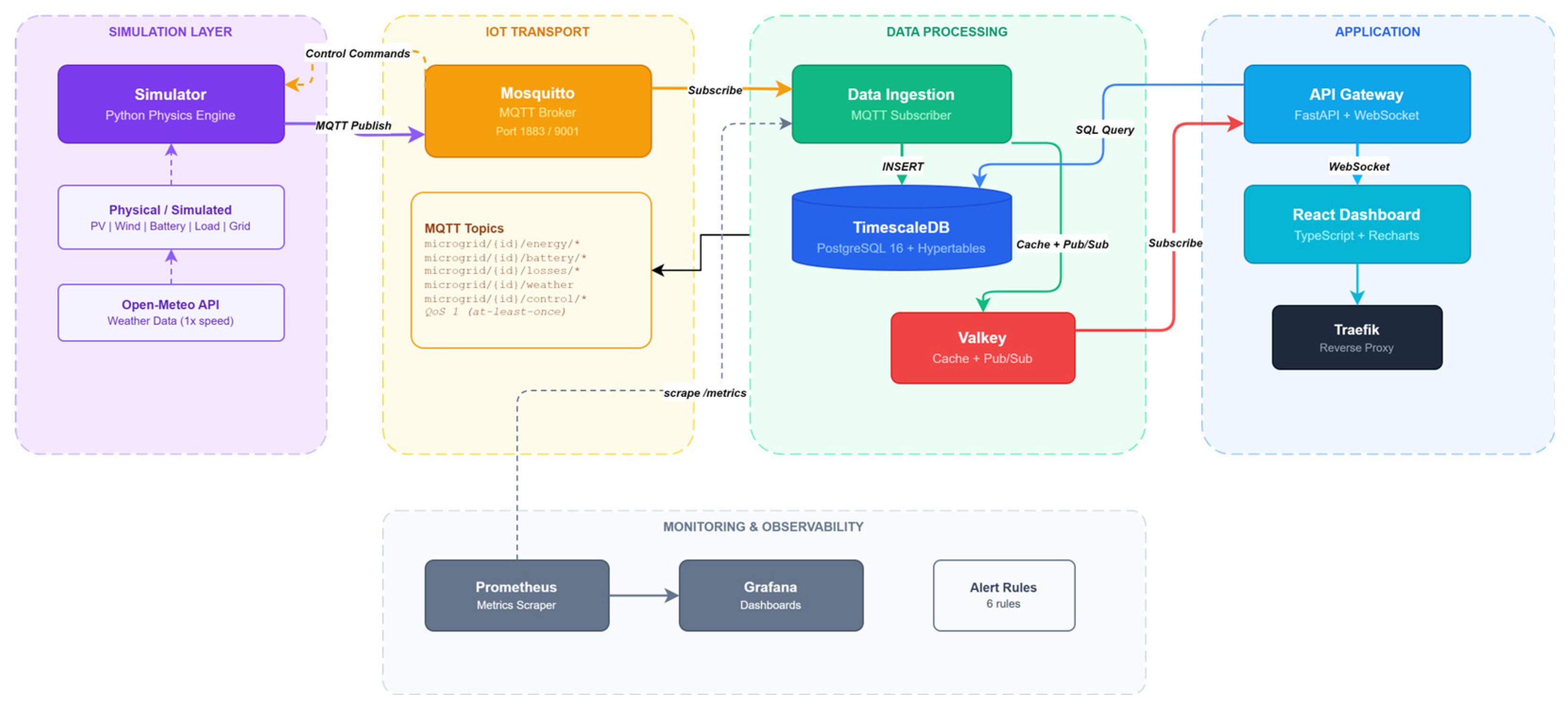
Figure 2.
12-step simulation pipeline flowchart.
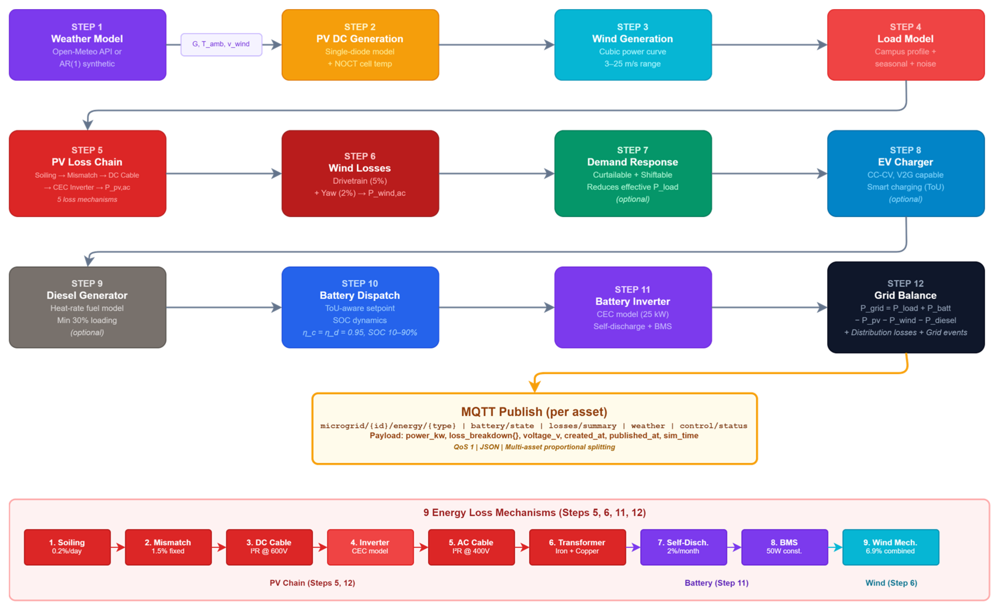
Figure 3.
PV loss chain block diagram (DC -> Soiling -> Mismatch -> DC Cable -> Inverter -> AC).
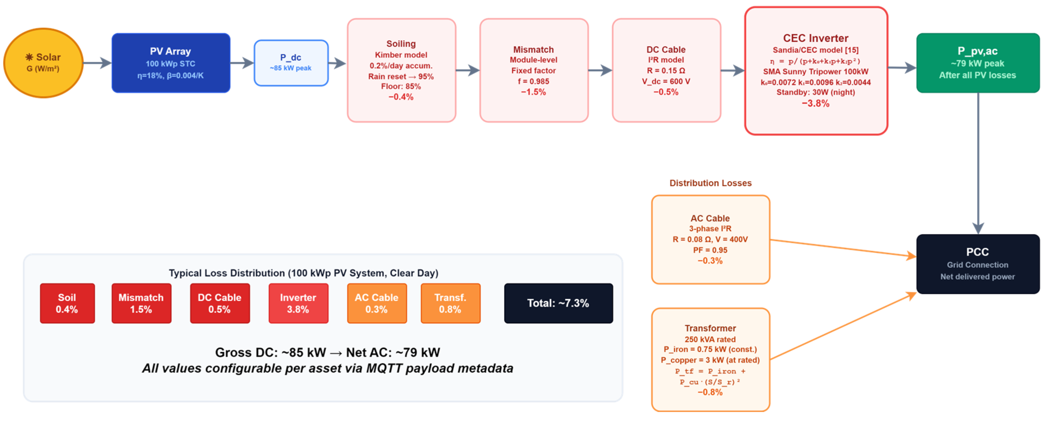
Figure 4.
MQTT topic hierarchy tree diagram.
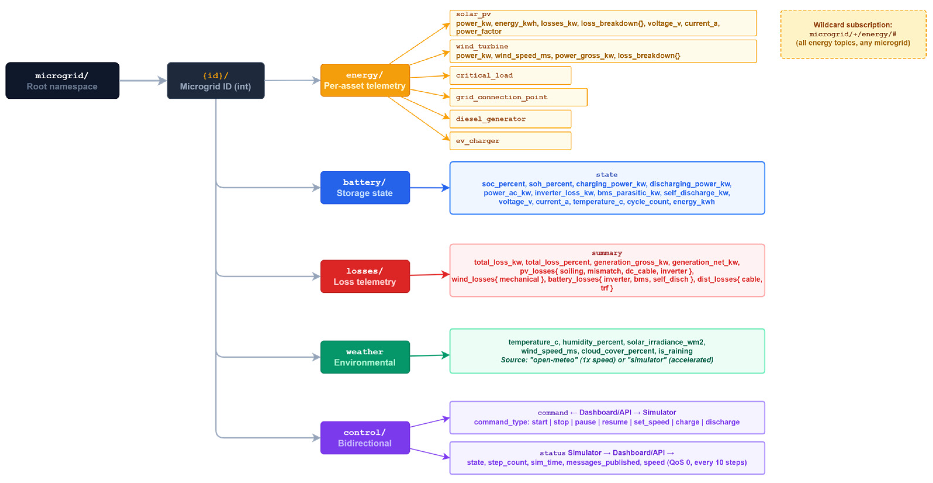
Figure 5.
Dashboard screenshot.
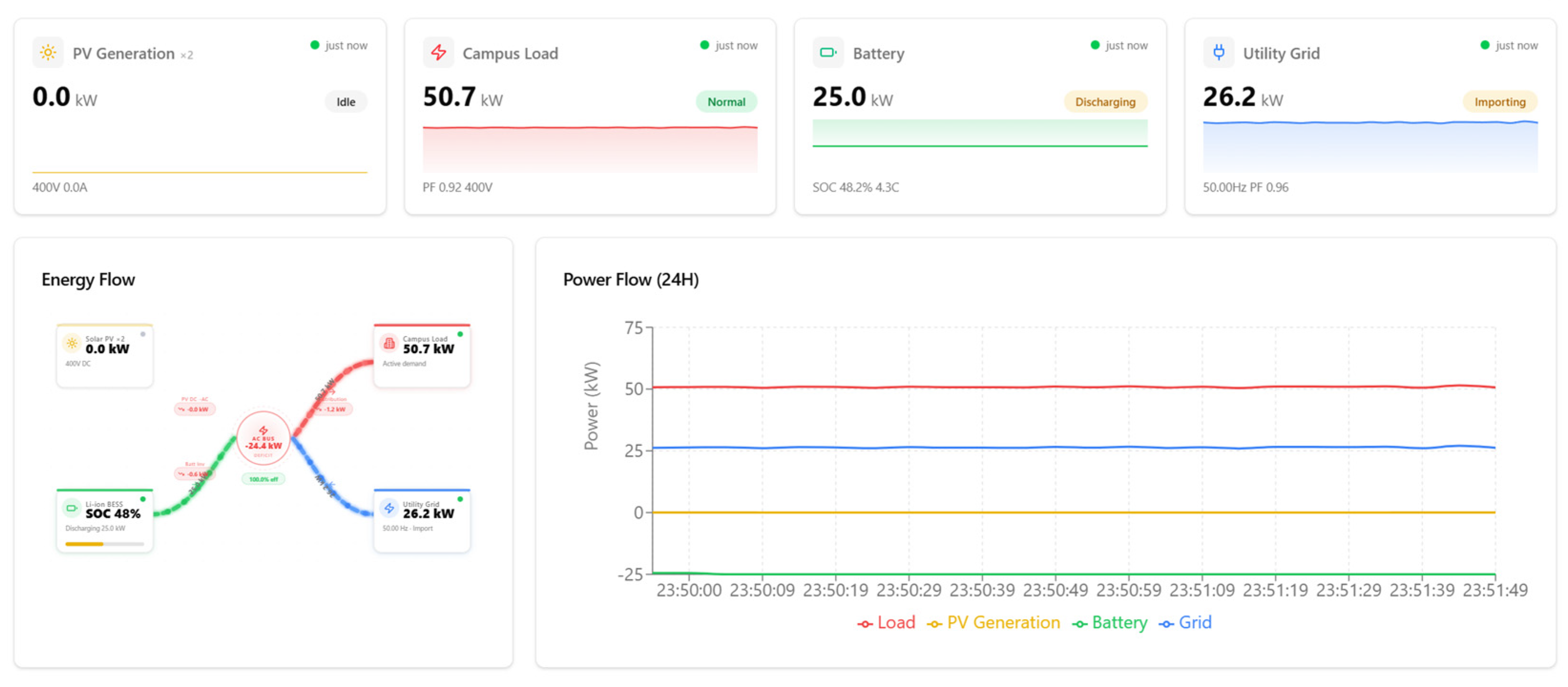
Figure 6.
The loss waterfall chart screenshot.
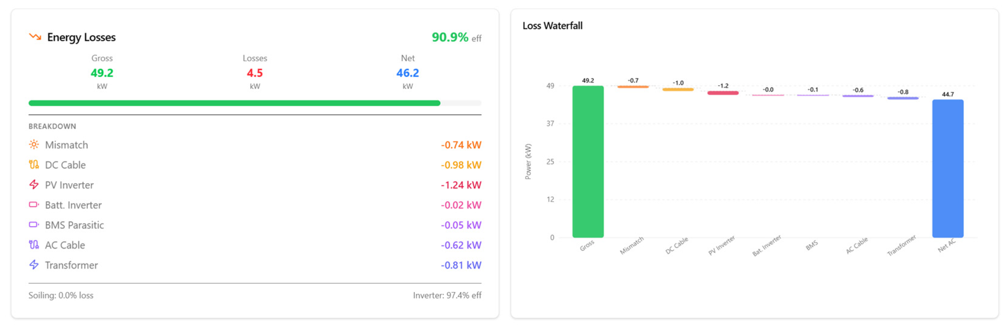
Figure 7.
Cumulative distribution function.
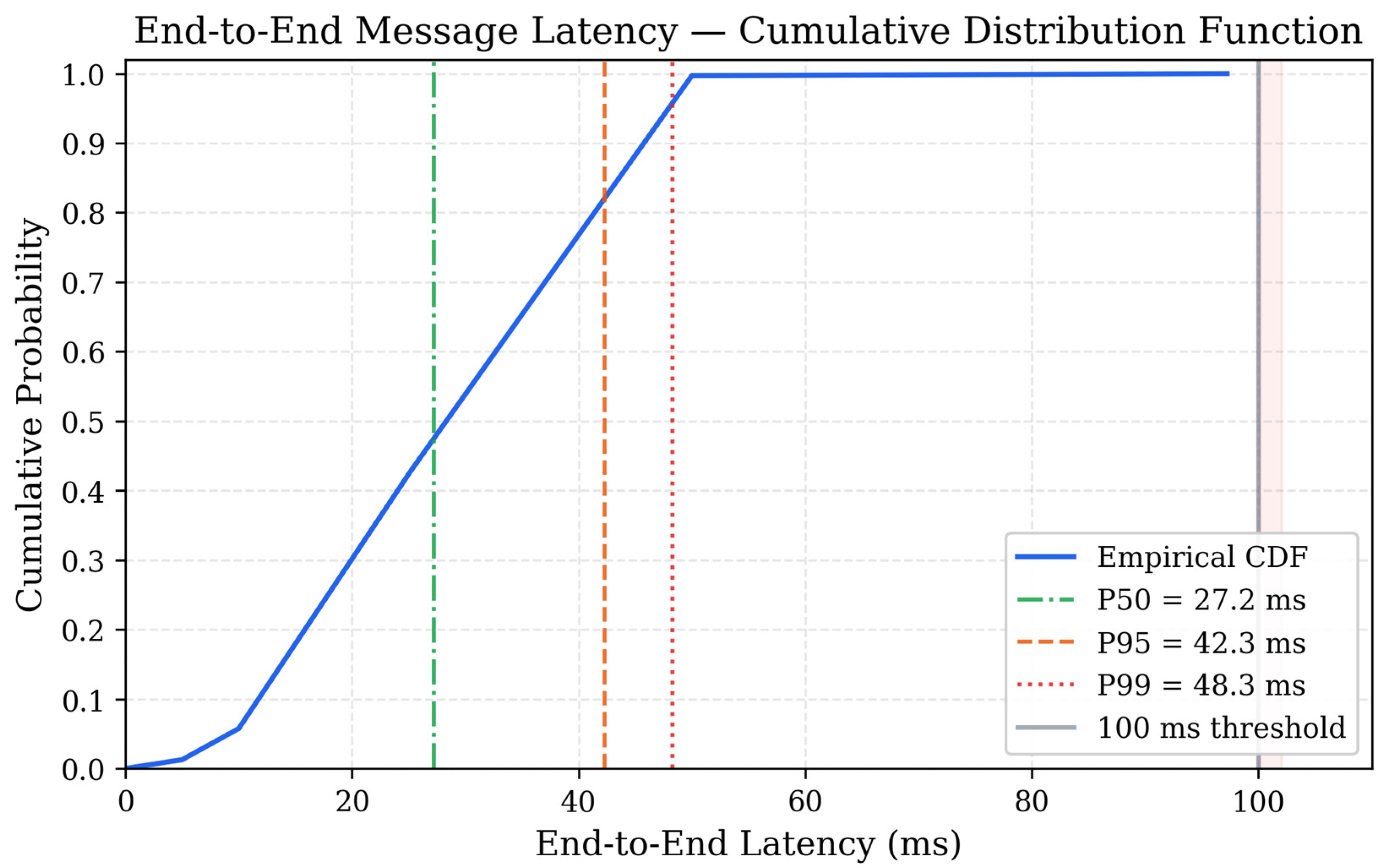
Figure 8.
Message throughput over time.
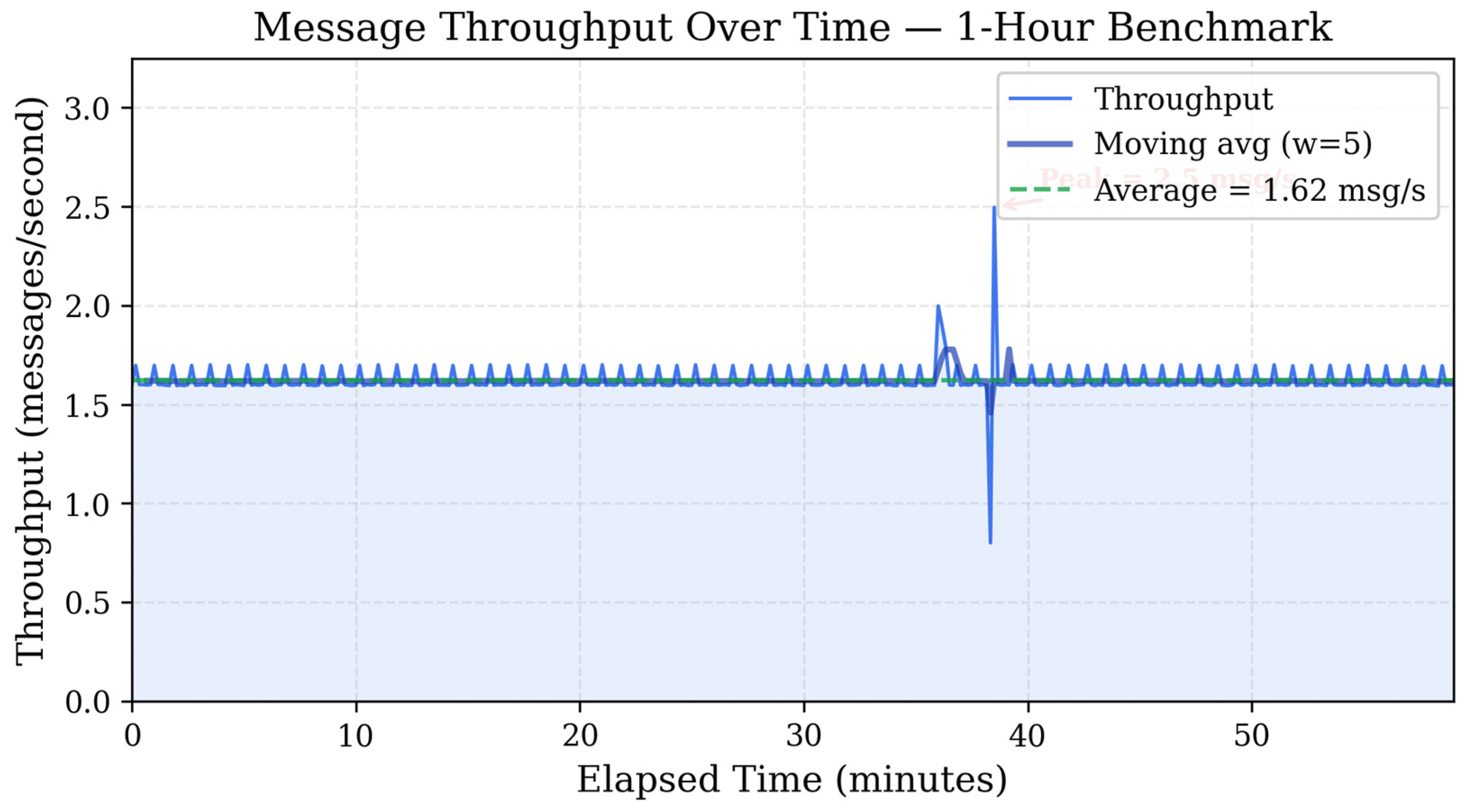
Figure 9.
PV energy loss waterfall.
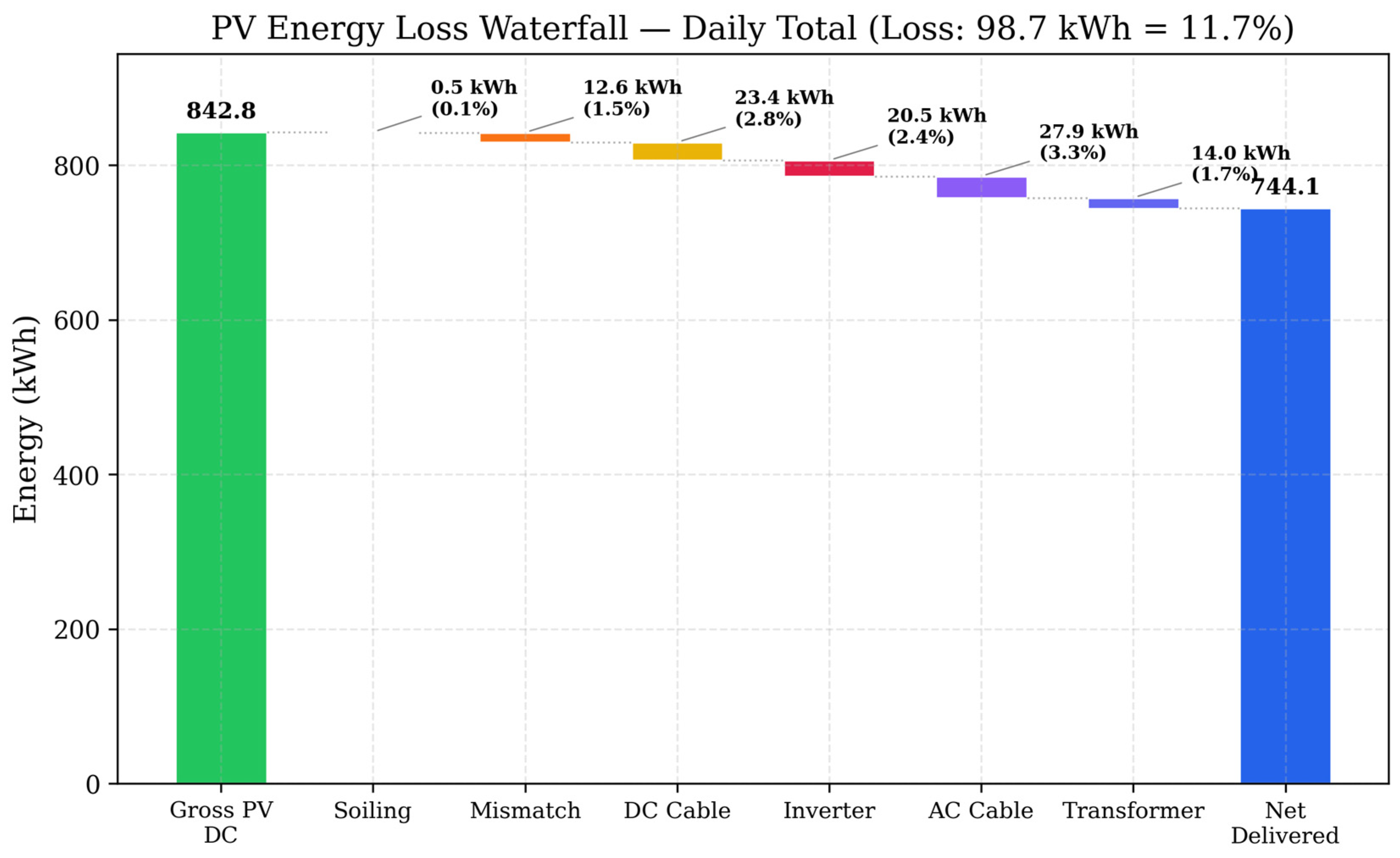
Figure 9.
Hourly loss breakdown by Mechanism.
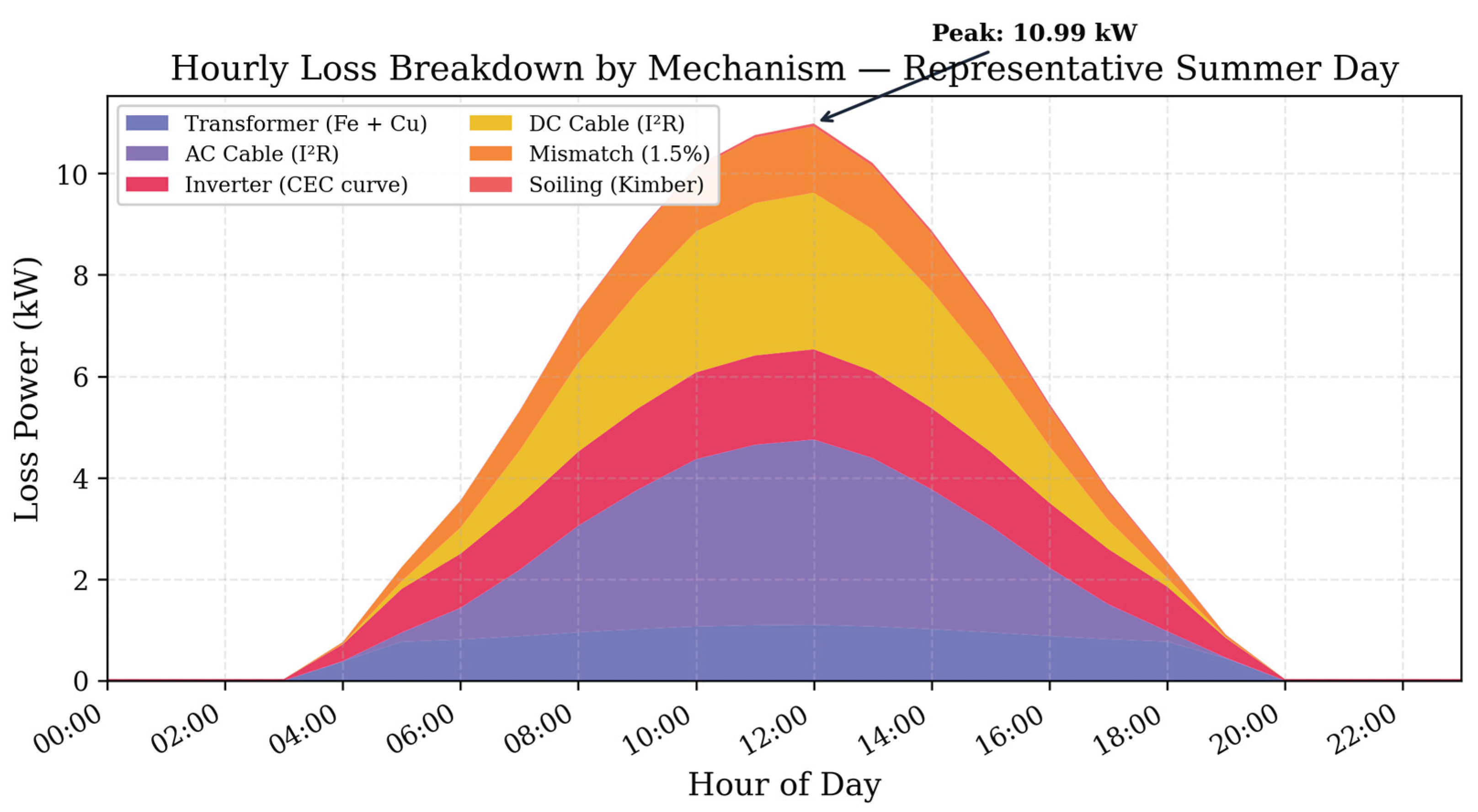
Table 3.
MQTT message schemas.
| Topic Pattern | Key Payload Fields | QoS | Rate | Avg Size |
|---|---|---|---|---|
| `microgrid/{id}/energy/{type}` | power_kw, energy_kwh, losses_kw, loss_breakdown, voltage_v, current_a, power_factor, frequency_hz, reactive_power_kvar | 1 | Per step | 374–604 B |
| `microgrid/{id}/battery/state` | soc_percent, soh_percent, charging_power_kw, discharging_power_kw, inverter_loss_kw, bms_parasitic_kw, temperature_c, cycle_count | 1 | Per step | 523 B |
| `microgrid/{id}/losses/summary` | total_loss_kw, total_loss_percent, generation_gross_kw, generation_net_kw, pv_losses{}, wind_losses{}, battery_losses{}, distribution_losses{} | 1 | Per step | 706 B |
| `microgrid/{id}/weather` | temperature_c, humidity_percent, solar_irradiance_wm2, wind_speed_ms, cloud_cover_percent, is_raining | 1 | Per step | 397 B |
| `microgrid/{id}/control/command` | command_type, parameters, target_asset_id | 1 | On demand | Variable |
| `microgrid/{id}/control/status` | state, step_count, sim_time, messages_published | 0 | Every 10 steps | 247 B |
Table 4.
End-to-End Latency Results (Aggregate).
| Metric | Value |
|---|---|
| P50 (average) | 27.2 ms |
| P50 (maximum) | 27.7 ms |
| P95 (average) | 42.3 ms |
| P95 (maximum) | 46.4 ms |
| P99 (average) | 48.3 ms |
| P99 (maximum) | 74.8 ms |
| Messages under 50 ms | 96.1% (5,610 / 5,840) |
| Messages under 100 ms | 100.0% (5,840 / 5,840) |
| Messages over 100 ms | 0 |
Table 5.
Per-Topic Latency Breakdown.
| Topic | Message Count | Rate (msg/min) | Avg. Latency (ms) | Avg Payload Size (B) |
|---|---|---|---|---|
| control/status | 75 | 1 | 1.01 | 247 |
| energy/solar_pv | 1474 | 24 | 15.09 | 604 |
| energy/wind_turbine | 737 | 12 | 21.65 | 485 |
| energy/critical_load | 737 | 12 | 25.83 | 374 |
| energy/grid_connection_point | 737 | 12 | 30.00 | 524 |
| battery/state | 737 | 12 | 30.73 | 523 |
| weather | 737 | 12 | 36.71 | 397 |
| losses/summary | 737 | 12 | 39.53 | 706 |
Table 6.
Platform Comparison.
| Platform | Open Source | Simulator | MQTT | Dashboard | Loss Model | Container | Benchmark |
|---|---|---|---|---|---|---|---|
| This Work | Yes | 12-step, 9 losses | Hierarchical | React + WS | Itemized, real-time | Docker x 12 | P50/P95/P99 |
| OpenEMS [29] | Yes | No | No | Partial | No | Partial | No |
| VOLTTRON [31] | Yes | No | No | No | No | No | No |
| Eclipse Ditto [32] | Yes | No | Generic | No | No | Yes | No |
| Cognitive DT [2] | No | Proprietary | Custom | Custom | Partial | Unknown | Cost only |
| pymgrid [11] | Yes | Basic | No | No | No | No | No |
| pvlib [12] | Yes | PV only | No | No | PV Only | No | No |
| ThingsBoard [33] | Yes (CE) | No | Yes | Generic | No | Yes | No |
| Hamid et al. [14] | No | MATLAB | No | No | PV only | No | No |
| Izquierdo et al. [28] | Yes | No | No | Partial | No | No | No |
Disclaimer/Publisher’s Note: The statements, opinions and data contained in all publications are solely those of the individual author(s) and contributor(s) and not of MDPI and/or the editor(s). MDPI and/or the editor(s) disclaim responsibility for any injury to people or property resulting from any ideas, methods, instructions or products referred to in the content. |
© 2026 by the authors. Licensee MDPI, Basel, Switzerland. This article is an open access article distributed under the terms and conditions of the Creative Commons Attribution (CC BY) license (http://creativecommons.org/licenses/by/4.0/).
Copyright: This open access article is published under a Creative Commons CC BY 4.0 license, which permit the free download, distribution, and reuse, provided that the author and preprint are cited in any reuse.


