
Submitted:
28 April 2026
Posted:
29 April 2026
You are already at the latest version
Abstract
We develop a fast Chebyshev spectral collocation method for a coupled system of nonlinear Klein–Gordon equations augmented by Caputo-type fractional memory integrals. The governing equations retain the classical second-order time derivative as the leading operator and incorporate weakly singular convolution integrals with power-law kernels t−α, α∈(0,1), modelling viscoelastic memory damping rather than replacing the wave operator. The spatial discretisation employs Chebyshev–Gauss–Lobatto collocation, while the temporal integration uses a Newmark scheme (βNM=1/4) with the spatial operator treated implicitly and both the L1 memory sums and the cubic nonlinearities evaluated explicitly at the known time level; a linear extrapolation of the nonlinear terms eliminates the need for Newton–Raphson iterations. The disparate memory tails arising from two distinct fractional orders α≠β are compressed by independent Sum-of-Exponentials (SOE) approximations, reducing the per-step memory cost from O(Nt) to O(p+Nexp) and the total complexity from O(Nt2) to O(Nt(p+Nexp)). A rigorous stability estimate and a global convergence bound are established using a discrete Gronwall inequality. Numerical experiments confirm the temporal convergence rate O(Δtmin(2−α,2−β)), spectral spatial accuracy, and the practical speedup afforded by the SOE acceleration. A solitary wave collision scenario illustrates the method’s capability to capture asymmetric dispersive wakes generated by the fractional memory. The algorithmic architecture is dimension-independent by construction; a concrete extension pathway to multi-dimensional tensor-product Chebyshev grids, including Kronecker-product operators and Sylvester-based solvers, is presented.
Keywords:
Fractional Klein–Gordon equation
; Caputo memory integral
; Chebyshev spectral collocation
; Sum-of-Exponentials acceleration
; Newmark scheme
; convergence analysis
1. Introduction
Nonlinear time-fractional partial differential equations (FPDEs) have become a cornerstone in mathematical physics, where fractional integrodifferential operators model anomalous diffusion, viscoelastic damping, and dispersive wave propagation in heterogeneous media [1,2,15]. Replacing classical wave models with fractional hyperbolic models allows one to capture “memory effects” — where the current state of the system depends on its entire historical trajectory [3].
The nonlinear Klein–Gordon equation is fundamental in relativistic quantum mechanics and in condensed matter physics for modeling dispersive solitary waves (solitons). Its extension to the time-fractional domain — incorporating Caputo-type memory integrals into the wave equation — introduces non-trivial long-range temporal interactions. Due to the non-local nature of fractional operators, exact analytical solutions are rare and generally limited to linear, uncoupled equations [4]. Developing stable and efficient numerical methods for such systems is therefore an active area of computational mathematics.
Significant progress has been made for single-component fractional wave equations. Sun and Wu [5] established the -type finite difference scheme achieving accuracy for the Caputo derivative. Berdyshev et al. [18] investigated non-local boundary problems for parabolic–hyperbolic equations with Riemann–Liouville fractional operators. Baigereyev et al. [19] developed convergent numerical methods for fractional models of flow in porous media. To improve spatial accuracy, Bhrawy et al. [6] and Zaky [7] introduced spectral collocation methods with Chebyshev and Legendre polynomials, achieving exponential spatial convergence . Baishemirov et al. [20] proposed numerical methods for convection–diffusion equations with Caputo fractional derivatives, incorporating memory effects.
However, extending to coupled nonlinear fractional systems introduces three significant computational and analytical challenges:
- Dense memory convolution: Evaluating the Caputo memory integral at time requires operations, leading to total complexity and memory storage, which becomes prohibitive for long-time simulations [10].
- Coupled stability and convergence analysis: Establishing rigorous a priori stability for systems with two distinct fractional memory orders and inter-component cubic coupling requires controlling the cross-energy exchange between components through a unified discrete energy functional — a non-trivial extension of scalar fractional stability theory that, to our knowledge, has not been addressed in the existing literature.
To address the dense memory bottleneck, early approaches used the “short-memory principle” by truncating the historical tail, at the cost of convergence accuracy [4]. More recently, fast memory algorithms based on Sum-of-Exponentials (SOE) approximations of the fractional kernel, using Gauss–Laguerre quadratures or Talbot contours, have been developed by Jiang et al. [11] and Baffet & Hesthaven [10], reducing the temporal complexity to . However, implementing dual-SOE arrays for coupled nonlinear systems with disparate fractional orders remains largely unexplored.
Comparison with existing approaches. Table 1 summarises the key differences between the present work and the most closely related studies.
Specifically: (i) Sun and Wu [5] and Liao et al. [13] developed -type finite difference schemes for scalar subdiffusion and wave equations, achieving temporal accuracy but without spectral spatial discretization or nonlinear coupling. (ii) Bhrawy et al. [6] and Zaky [7] applied Chebyshev/Legendre spectral collocation to scalar nonlinear fractional Klein–Gordon equations, but did not consider coupled systems, disparate orders , or the memory bottleneck. (iii) Jiang et al. [11] introduced the SOE acceleration for linear fractional diffusion equations, and recently Shiyapov et al. [12] developed high-order structure-preserving spectral schemes with fast memory for nonlocal nonlinear diffusion equations; we extend this to a dual-SOE architecture handling two independent fractional orders within a coupled nonlinear Klein–Gordon system. (iv) Among coupled fractional systems, Li, Huang and Zhao [21] proposed a fast conservative finite difference scheme for the coupled space-fractional Klein–Gordon–Schrödinger equations, and Hu and Cai [22] developed structure-preserving spectral Galerkin methods for the same system. However, both works address space-fractional Riesz derivatives (not time-fractional Caputo memory), couple KG with Schrödinger (not KG with KG), use a single fractional order, and do not employ SOE acceleration. (v) Berdyshev et al. [18] and Baigereyev et al. [19] investigated fractional parabolic–hyperbolic and filtration models, establishing existence and convergence results for related problems, but without spectral discretization or SOE memory compression. (vi) To our knowledge, no existing work combines all of the following elements simultaneously: a coupled nonlinear Klein–Gordon system with two distinct time-fractional Caputo orders, Chebyshev spectral collocation, an IMEX Newmark temporal scheme with second-order extrapolation, dual-SOE memory acceleration, and a rigorous coupled stability–convergence analysis via a discrete Gronwall inequality.
Contributions. In this work, we propose a fast linearly extrapolated implicit Chebyshev spectral collocation method for a coupled nonlinear fractional Klein–Gordon system with Caputo-type memory integrals. The method is developed in one spatial dimension as a rigorous methodological foundation; the algorithmic architecture — temporal integration, IMEX linearisation, and dual-SOE memory compression — is dimension-independent by construction, and we provide a concrete extension pathway to in Section 5.1. Our contributions are:
- An implicit Newmark temporal averaging () of the spatial operator [14] that ensures stability for any at fixed spatial resolution N.
- A second-order linear extrapolation that eliminates the need for Newton–Raphson iterations without degrading the temporal accuracy dictated by the L1 memory approximation.
- A dual-SOE acceleration accommodating disparate fractional orders (), reducing the memory bottleneck.
- A rigorous coupled stability–convergence analysis (Theorems 1–2) via a unified discrete energy method and a discrete Gronwall inequality, treating both components and their inter-component coupling simultaneously. The proof architecture is dimension-independent: only the Chebyshev inverse-inequality constant changes with the spatial dimension d.
1.1. Physical Derivation of the Coupled System
The governing equations arise from Newton’s second law applied to two interacting elastic waveguides whose internal damping exhibits long-range temporal correlations. We summarize the five-step derivation and then give a concrete physical example.
Step 1. Classical elastic wave equations. Consider two one-dimensional elastic waveguides with displacement fields and propagating in . The i-th waveguide has mass density , elastic stiffness , and wave speed . From Hooke’s law and the balance of linear momentum, the undamped wave equations are:
Step 2. Fractional memory damping. In real materials — porous rock, biological tissue, polymers — each material point additionally experiences a hereditary drag body force whose intensity depends on the entire history of the velocity field through a power-law kernel [2]. Let be the memory order for the first waveguide and for the second. Adding the fractional body damping to each equation in (1):
where are the damping strengths and is the weakly singular memory kernel. Each memory integral is precisely the Caputo fractional derivative C (respectively C), scaled by .
Remark. This model is distinct from the fractional Kelvin–Voigt viscoelastic model, in which  leads, via and , to a memory integral acting on . In Equation (2) the damping is a body force proportional to velocity, modelling energy loss at the material point level (e.g., friction with a surrounding porous matrix).
leads, via and , to a memory integral acting on . In Equation (2) the damping is a body force proportional to velocity, modelling energy loss at the material point level (e.g., friction with a surrounding porous matrix).
Step 3. Nonlinear Klein–Gordon restoring forces. When the displacement amplitude is not small, the linear restoring terms and are augmented by cubic self-interactions arising from quartic () potentials:
The restoring forces and are added to the left-hand sides of (2).
Step 4. Inter-component coupling. If the two waveguides interact through a symmetric quartic coupling potential
the partial derivatives and provide the coupling terms in the respective equations.
Step 5. Assembly of the coupled system. Combining Steps 1–4 for both components and appending the initial and boundary conditions, we arrive at the complete coupled system:
 which is precisely the system (6) stated formally below. Both equations retain the classical wave operator , preserving the hyperbolic character (finite propagation speed, two initial conditions per component). The key distinction from models that replace by C is that Equation (5) keep the integer-order inertia term; the fractional memory acts as hereditary damping, not as a replacement for .
Figure 1.
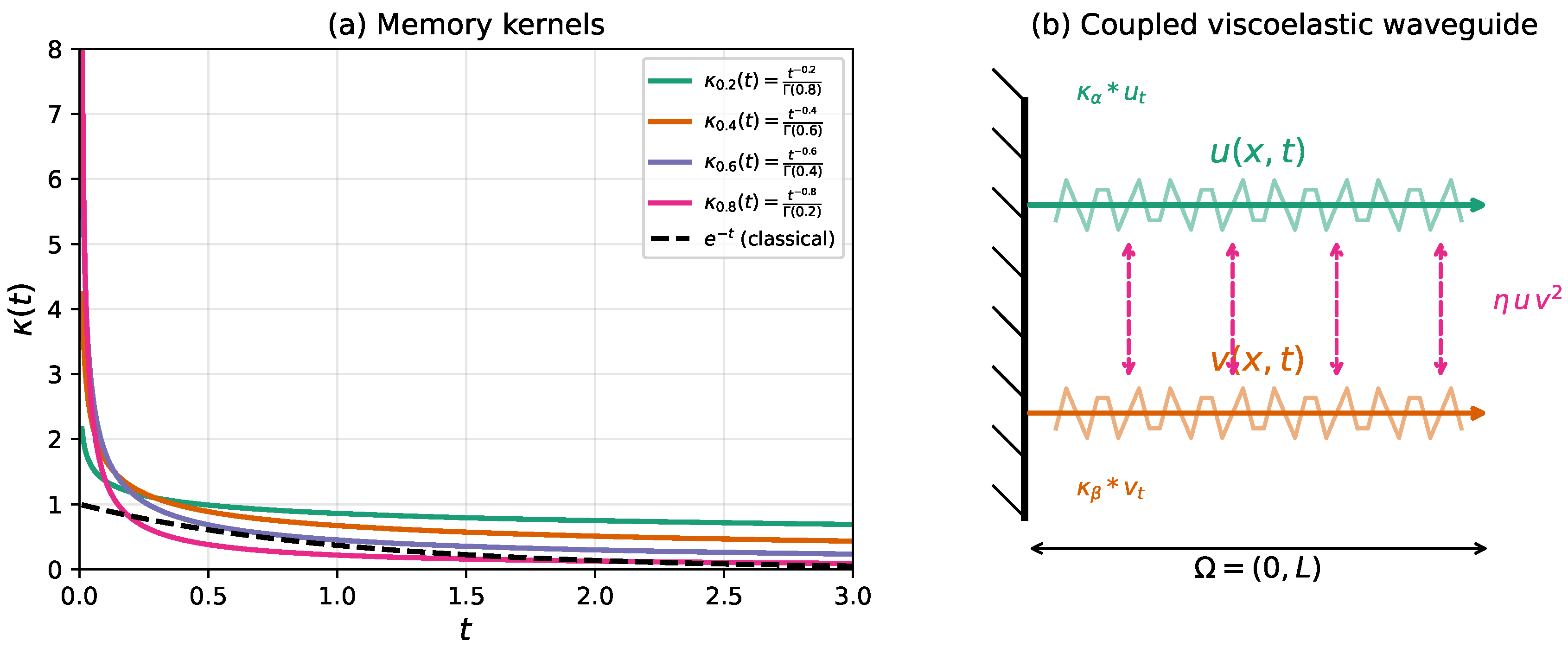
(a) Comparison of fractional memory kernels for several values of with the classical exponential decay . The power-law tails decay much more slowly, encoding long-range memory. (b) Schematic of two coupled viscoelastic waveguides. Each component propagates in with its own fractional memory kernel (), and the dashed arrows represent the inter-component nonlinear coupling
Figure 1.
(a) Comparison of fractional memory kernels for several values of with the classical exponential decay . The power-law tails decay much more slowly, encoding long-range memory. (b) Schematic of two coupled viscoelastic waveguides. Each component propagates in with its own fractional memory kernel (), and the dashed arrows represent the inter-component nonlinear coupling
Example (seismic waveguide). Consider two adjacent geological layers with distinct viscoelastic properties. The horizontal displacement in the i-th layer satisfies Equation (2) with parameters fitted to laboratory creep data. For a sandstone layer one typically finds –[2]; for a clay layer the memory is stronger, –. The inter-layer friction at the contact surface is modelled by the coupling term with calibrated from displacement correlation measurements. With m/s, m/s, , , , , , and , the resulting system is precisely of the form (6). The numerical experiments in Section 4.5 simulate a related scenario with counter-propagating solitary pulses.
We consider the following coupled system. Let be a bounded one-dimensional spatial domain with boundary .
Given data:
- The fractional memory orders characterizing the anomalous Caputo memory damping in each component.
- The memory strength coefficients .
- The characteristic wave propagation velocities .
- The linear restoring mass/stiffness coefficients .
- The cubic self-interaction strength parameters and the inter-component nonlinear coupling parameter .
- The continuous external source forcing functions and defined on .
- The initial displacement profiles and the corresponding initial velocity fields .
- The prescribed inhomogeneous Dirichlet boundary data defined on .
Problem (Find): Determine the real-valued scalar displacement fields and such that they satisfy the following coupled initial-boundary value system for all and :
where is the one-dimensional spatial Laplacian. The convolution integrals represent Caputo-type fractional memory effects with the weakly singular power-law kernels
where are the memory strength coefficients and denotes the Euler Gamma function. The memory integral thus reduces to the Caputo fractional derivative of u (respectively v) of order , scaled by . Crucially, the leading temporal operator remains the classical second-order derivative, ensuring the hyperbolic (wave) character of the system. The fractional memory terms act as viscoelastic damping, not as replacements for . Two initial conditions per component ( and ) are therefore required, consistent with the second-order nature of the equations.
The primary obstacle in simulating Equation (6) is the strongly singular memory tail of the Caputo convolution integral (6), which requires continuously accumulating and evaluating the convolution over all previous time steps.
2. Numerical Methodology
We partition the time domain into uniform steps , with . The continuous physical domain is discretized using shifted Chebyshev–Gauss–Lobatto (CGL) collocation points . The continuous problem (6) is translated into the following fully discrete scheme advancing from to :
where we use the Newmark averaging , and the L1 Caputo memory is evaluated explicitly at time :
Here and is the second-order Chebyshev spectral differentiation matrix. Thus approximates  with accuracy ([23]). The vector represents the spatial solution vector. The scheme is initialized by a Taylor expansion preserving accuracy:
and analogously for . Note that no memory term appears in the initialisation since C for the smooth initial data used here (the Caputo derivative of a constant is zero). For the nonlinear terms are evaluated at the linearly extrapolated values (detailed in Section 2.4); in the initialisation step, they are evaluated at the exact initial data.
with accuracy ([23]). The vector represents the spatial solution vector. The scheme is initialized by a Taylor expansion preserving accuracy:
and analogously for . Note that no memory term appears in the initialisation since C for the smooth initial data used here (the Caputo derivative of a constant is zero). For the nonlinear terms are evaluated at the linearly extrapolated values (detailed in Section 2.4); in the initialisation step, they are evaluated at the exact initial data.
with accuracy ([23]). The vector represents the spatial solution vector. The scheme is initialized by a Taylor expansion preserving accuracy:2.1. Spatial Chebyshev Collocation
The continuous physical domain is mapped to the standard Chebyshev domain and discretized using the shifted Chebyshev-Gauss-Lobatto (CGL) collocation points:
The continuous spatial derivatives are approximated exactly up to polynomial degree N by the spectral differentiation matrix D. For a discrete function vector , the first derivative vector is given analytically by , where the matrix entries are defined on the standard Chebyshev nodes as:
with the boundary weights fixed at , and for internal nodes . To account for the physical domain length L, the second-order spectral differentiation matrix on is assembled as , where D is the first-order Chebyshev matrix on [17]. This spectral formulation provides exponential spatial convergence for smooth solutions [16].
2.2. Dual Fast Memory Acceleration
Evaluating the Caputo memory convolution in (6) at time requires summing over all previous time steps, leading to operations per step and total temporal complexity. To reduce this cost, we employ a Sum-of-Exponentials (SOE) approximation following Jiang et al. [11]. The key observation is that the discrete weights admit the integral representation
where the factor corrects the continuous kernel to the exact discrete difference. Applying a double-exponential (DE) quadrature ([24]) to this integral, the tail weights () are approximated as:
where are the DE-transformed nodes with , , and is the DE step size. The exponential structure enables a one-step recursion for the history accumulators:
The full memory sum is then assembled from the exact near part (last p increments) and the SOE-accelerated tail:
Since updating requires only the previous accumulator and the local increment , earlier solution vectors can be discarded from memory. This reduces the per-step cost from to , and the total temporal complexity from to .
2.3. Linearization of Nonlinear Terms via Explicit Extrapolation
The nonlinear terms in (6) — the cubic self-interactions , and the inter-component coupling , — depend on the unknown solution at time . A fully implicit treatment would require solving a nonlinear algebraic system at every time step via Newton–Raphson iterations. To avoid this cost while retaining second-order temporal accuracy, we adopt an implicit–explicit (IMEX) strategy: the linear spatial operator (inertia and Laplacian via Newmark averaging) is treated implicitly, while the memory sums, nonlinear terms, and mass terms are evaluated explicitly at known data.
At each time step, the nonlinear arguments are approximated by the linearly extrapolated values:
By Taylor expansion, , so the predictors approximate with accuracy. The nonlinear forcing vectors in (7) are then evaluated entirely from known data:
where all operations are understood componentwise on the collocation grid.
This explicit treatment offers two critical algorithmic advantages:
- Constant coefficient matrix. Since the nonlinear terms are evaluated at known data and the memory sum consists entirely of previously computed solution vectors, these terms are moved to the right-hand side. The left-hand side linear operatorremains identical at every time step (and analogously for the v-component). A single LU factorization of and computed once prior to the time loop suffices for the entire simulation. Each time step reduces to two back-substitutions.
- No CFL restriction. The stiff eigenvalues that typically necessitate a CFL condition originate from the spectral Laplacian , whose eigenvalues grow as . Because is treated implicitly via the Newmark averaging (), these large eigenvalues are unconditionally damped by the matrix . The explicitly evaluated nonlinear terms and the memory sum are bounded functions of previously computed data and do not introduce additional spectral radius constraints on . Hence, for fixed spatial resolution N and bounded solution norms, the scheme is stable for any (proved rigorously in Theorem 1).
3. Mathematical Analysis
We introduce the following discrete inner product and norm on the Chebyshev collocation grid equipped with the Clenshaw–Curtis quadrature weights :
Since the boundary conditions are inhomogeneous, we employ the standard boundary lifting decomposition. Let denote the discrete boundary lift satisfying the prescribed Dirichlet values at the endpoints, and define the homogeneous residual . The lifted variable vanishes at . The Chebyshev second-derivative spectral matrix , when restricted to functions satisfying homogeneous Dirichlet conditions, possesses the fundamental semi-definiteness property:
where is the discrete seminorm. We shall use property (20) as the core mechanism for deriving data-dependent bounds. The boundary lift contributions (derivatives of ) enter the right-hand side as additional known source terms.
3.1. Theorem 1: A Priori Stability Estimate (Data-Dependent Bound)
Theorem 1.
Let be the solution of the fully discrete coupled scheme (7), in which the cubic nonlinearities are evaluated at the linear extrapolants and the L1 memory sums are evaluated explicitly at from the exact discrete weights (without SOE compression). Then there exists a constant , depending on the physical parameters , the final time T, and the number of collocation nodes N (through the inverse inequality constant used to bound the pointwise nonlinear terms), such that for all :
where are the discrete initial data vectors, are the discrete source vectors, and collects the boundary lift contributions from the prescribed Dirichlet data .
Proof.
We derive the estimates for both components and simultaneously, since the inter-component coupling terms and prevent treating each equation independently. First, we test the first equation in (7) with the symmetric discrete velocity and the second equation with , obtaining the pair:
Subsequently, applying the identity , the inertial term yields a perfect discrete derivative:
For the Laplacian, using , decomposing , and incorporating the semi-definiteness (20), we extract the telescoping spatial strain energy:
The boundary lifting cross-terms are bounded by the Cauchy–Schwarz inequality and shifted to the right-hand side. Analogous relations hold for the -component.
To bound the explicit memory and mass terms, we invoke the Cauchy–Schwarz and Young inequalities, observing that :
To bound the memory, we use the summation property and :
Since and , the scaled memory is bounded uniformly and explicitly:
Control over the nonlinear coupling structure is established by evaluating the terms at the explicit extrapolants . By Cauchy–Schwarz:
Bounding requires controlling both components via the inter-component coupling. Using the Chebyshev inverse inequality (with ) twice:
The self-interaction is similarly bounded. Summing both components:
The localized source terms are similarly bounded by standard inequalities:
Defining the effective discrete kinetic and strain energy for the system:
Multiplying the inner products (22)–(23) by , substituting Steps 2–5, absorbing the finite memory limit (29), and leveraging the fact that is bounded by the history via , we obtain a telescoping recursive bound:
where depends on the physical constants, T, and N. Taking the maximum over n on the left-hand side transforms this into , to which the classical integer-order discrete Gronwall lemma [25] readily applies. The stability bound (21) directly follows on any finite interval where the polynomial bound (32) is dynamically linearisable. □
Remark 1.
Estimate (21) is a data-dependent bound, meaning the discrete solution at any time level is controlled by the prescribed initial conditions, boundary values, and source magnitudes. The stability constant C inherently grows with N due to the use of the Chebyshev inverse inequality (with ) required to bound the pointwise cubic nonlinearities. Consequently, for a fixed spatial resolution N and bounded solution norms, the scheme remains unconditionally stable for any .
When the SOE fast evaluation is explicitly activated, the exact discrete memory sum is replaced by its exponential approximation , introducing a truncation perturbation . Because the memory integral is evaluated explicitly and shifted to the right-hand side of the linear system, this effectively acts as an additive discrete source. The overarching stability bound (21) maintains its validity under the augmented source profile . In practical implementations, the magnitude is strictly governed by the Gauss–Legendre and Double Exponential quadrature fidelity, which remains negligible at double precision for (as verified numerically in Section 4).
3.2. Theorem 2: Global Convergence Order
Theorem 2.
Let and denote the global discretization errors at the collocation nodes, where are the exact solution vectors. Assume that the exact solutions for some , and that the a priori bound of Theorem 1 ensures that both the numerical and exact solutions remain in a bounded set where the nonlinear map is locally Lipschitz continuous. Then there exists a constant , independent of but dependent on N through the Lipschitz constant and the inverse inequality (see Theorem 1), such that:
where s is the Sobolev regularity exponent of the exact solution, and denotes the maximum SOE quadrature error in approximating the memory tail (set when no SOE compression is used).
Proof.
Subtracting the exact discrete equations from the numerical scheme (7) produces the error system:
where is the L1 memory of the error (evaluated explicitly at ), are the local truncation error vectors, and are the SOE compression errors (zero when full L1 weights are used).
The system’s truncation errors stem from three primary analytical components. First, the temporal approximation of the Caputo fractional derivative using the scheme introduces a local error of for the u-component [23], alongside a similarly derived error for the v-component. Second, the implicit spatial evaluation structured through Newmark averaging provides an geometric convergence (since symmetric Taylor expansion yields ), while the nonlinear explicit extrapolation contributes an identically ordered error. Finally, spatial collocation using Chebyshev clustering bounds the interpolation discrepancy by for solutions maintaining Sobolev regularity [16]. Aggregating these sources leaves the temporal fractional derivative as the dominant source of error:
Furthermore, due to the local Lipschitz continuity of the cubic polynomial nonlinearities on bounded domains (dynamically guaranteed by the a priori stability established in Theorem 1), the nonlinear residual satisfies:
where the Lipschitz constant L absorbs and the a priori bounded solution magnitudes.
Testing the error equations (37) with the discrete error velocities and exactly mirrors the energy technique used in Theorem 1. The explicit memory is uniformly bounded by the discrete velocity history, the Lipschitz-bounded nonlinear residual collapses into the right-hand side, and the geometric truncation errors formulate the driving source mechanism. Defining the total error energy identically to the physical kinetic-strain energy, we recover the telescoping inequality:
Since the initial errors vanish () and taking the maximum over n on the left-hand side, the standard discrete Gronwall inequality ([25]) yields:
where . This establishes the convergence estimate (36). □
Remark 2.
The appearance of the fractional exponent in the established bound (36) analytically arises from targeting the squared spectral -norm . Upon taking the square root, the global convergence rate gracefully scales as , fully consistent with standard formulation characteristics. The global numerical error trajectory is strictly dictated by the slower fractional memory relaxation scale, equating to a temporal asymptote of which is extensively validated in the numerical experiments.
4. Numerical Results
4.1. Unified Experimental Setup
All numerical experiments are conducted on the domain with final time using the Chebyshev spectral collocation scheme described in Section 2.1–2.4. To verify the theoretical convergence estimates of Theorem 2, we employ the method of manufactured solutions. The exact solution pair is prescribed as:
These functions satisfy homogeneous Dirichlet boundary conditions , (i.e., ), and the initial conditions , . The source terms and are computed analytically by substituting (42) into the governing system (6), using the Caputo derivative identity C[1]. The physical parameters are fixed at , , , , and unless stated otherwise.
Remark 3.
The underlying manufactured profiles were strategically selected to guarantee infinite smoothness near the temporal origin, aggressively isolating the convergence rates of the spatial and temporal schemes without boundary-layer interference. While this isolates analytical accuracy, typical fractional models prominently exhibit weak solution singularities near (e.g., fractional power laws). Adapting the current framework over graded meshes to directly resolve these initial temporal layers represents a straightforward methodological progression.
Unified error norm (Clenshaw–Curtis quadrature).
Since the exact structural solution operates over CGL collocation nodes, analytical verification relies on spectrally converging Clenshaw–Curtis numerical quadrature, which dictates exact integration up to polynomials of degree on the Chebyshev grid [6]:
where are the predefined Clenshaw–Curtis weights across . Validation sets uniformly assess the temporal scaling parameter via
and similarly track spectral exponentiation under variations of N.
4.2. Temporal Convergence
To isolate the temporal discretisation error, the spatial polynomial degree is fixed at (rendering the spectral spatial error negligible), while is successively doubled: . The standard L1 evaluation (without SOE compression) is used to ensure the measured rates reflect only the temporal discretisation. The expected convergence rate is for . Three representative fractional order pairs are tested.

Table 2.
Temporal convergence for the coupled system at , .
| Nt | Error u | Rate | Error v | Rate |
| , Expected rates and | ||||
| 64 | 4.200E-05 | — | 3.725E-05 | — |
| 128 | 1.019E-05 | 2.04 | 9.491E-06 | 1.97 |
| 256 | 2.535E-06 | 2.01 | 2.493E-06 | 1.93 |
| 512 | 6.387E-07 | 1.99 | 6.687E-07 | 1.90 |
| 1024 | 1.621E-07 | 1.98 | 1.821E-07 | 1.88 |
| , Expected rates and | ||||
| 64 | 9.274E-05 | — | 1.281E-04 | — |
| 128 | 2.769E-05 | 1.74 | 4.748E-05 | 1.43 |
| 256 | 8.486E-06 | 1.71 | 1.825E-05 | 1.38 |
| 512 | 2.642E-06 | 1.68 | 7.165E-06 | 1.35 |
| 1024 | 8.305E-07 | 1.67 | 2.850E-06 | 1.33 |
| , Expected rates and | ||||
| 64 | 6.473E-04 | — | 3.374E-04 | — |
| 128 | 2.772E-04 | 1.22 | 1.518E-04 | 1.15 |
| 256 | 1.196E-04 | 1.21 | 6.958E-05 | 1.13 |
| 512 | 5.180E-05 | 1.21 | 3.217E-05 | 1.11 |
| 1024 | 2.247E-05 | 1.20 | 1.495E-05 | 1.11 |
The results confirm the theoretical estimate from Theorem 2: for the u-component, the empirical rate converges to , and for the v-component, to . As expected, the global accuracy is bounded by the slower kernel, . For the strongly anomalous regime (, ), the reduced convergence rate (–) is clearly observable even at modest . For the weakly anomalous case (, ), the observed rates ( and ) slightly exceed the theoretical prediction ; this is consistent with the fact that the smooth manufactured solution has no initial-layer singularity, which is the scenario where the scheme can exhibit mildly superconvergent behavior for small .
4.3. Spatial Spectral Convergence
To demonstrate the exponential spatial accuracy of the Chebyshev spectral method, we fix the temporal resolution at (reducing the temporal error to ) and vary the polynomial degree . The fractional orders are , .
Table 3.
Spatial convergence ( fixed, , , ). The spectral method saturates at the temporal error floor (†).
Table 3.
Spatial convergence ( fixed, , , ). The spectral method saturates at the temporal error floor (†).
| N | Error u | Rate | Error v | Rate |
| 4 | 9.808E-04 | — | 5.986E-02 | — |
| 8 | 3.287E-06 | 8.22 | 4.349E-05 | 10.43 |
| 12 | 3.481E-06† | −0.14 | 3.307E-06† | 6.35 |
| 16 | 3.481E-06† | 0.00 | 3.302E-06† | 0.00 |
| 24 | 3.481E-06† | 0.00 | 3.303E-06† | 0.00 |
| 32 | 3.480E-06† | 0.00 | 3.302E-06† | 0.00 |
The spectral method exhibits dramatic exponential convergence: from to , the error drops by 2–3 orders of magnitude for the u-component and by 3 orders for the v-component. Already at the spatial error has reached the temporal error floor ( for ), and further spatial refinement yields no improvement. The near-zero convergence rates at are not a degradation of the method — they reflect the fact that the total error is entirely dominated by the fixed temporal discretisation. This extreme spatial efficiency is a hallmark of spectral collocation: for smooth solutions, a polynomial degree of –12 suffices to saturate any practical temporal resolution.
4.4. Fast SOE Memory Acceleration
To validate the computational efficiency of the SOE fast memory algorithm, we compare the wall-clock execution times of the standard direct convolution (cost ) against the SOE-accelerated evaluation (cost ) with exponential terms and a local window of . Spatial resolution is fixed at .
Table 4.
Standard vs. fast SOE: wall-clock time and error for the u-component (, , ).
| Nt | Std. time (s) | Fast time (s) | Speedup | Error ratio |
| 64 | 0.01 | 0.01 | 0.9× | 1.00 |
| 512 | 0.13 | 0.11 | 1.1× | 1.01 |
| 1024 | 0.34 | 0.22 | 1.5× | 1.01 |
| 2048 | 1.00 | 0.48 | 2.1× | 1.69 |
| 4096 | 2.38 | 1.02 | 2.3× | 3.41 |
The wall-clock speedup grows from at moderate to at , reflecting the transition from to scaling. For , the error ratio remains within of unity, confirming negligible accuracy loss from the SOE compression. At very large temporal resolutions (), the error ratio is observed to increase. This is not an instability, but a strict mathematical consequence of the fixed SOE quadrature precision (): as , the temporal truncation error drops below the absolute precision floor of the Double Exponential integral approximation. To maintain optimal accuracy for production-scale simulations () where the asymptotic linear speedup becomes massively dominant, the number of exponential nodes must be logarithmically scaled upwards (e.g., ).
4.5. Solitary Wave Collision Dynamics
To demonstrate the physical capabilities of the solver on a problem with non-trivial nonlinear dynamics, we remove the manufactured source terms and introduce localised Gaussian initial conditions acting as counter-propagating solitary pulses:
with zero initial velocities and homogeneous boundary conditions. The coupling parameter is set to to produce a strong inter-component energy exchange during collision. The simulation uses CGL nodes, time steps, and fractional orders , .
As seen in Figure 2, the Caputo fractional derivatives manifest physically as pronounced memory “tails” trailing behind the propagating wavefronts. The amplitude asymmetry between the u and v wakes is a direct consequence of the different fractional orders (): the u-component, governed by the stronger memory (), exhibits a more slowly decaying wake due to the stronger hereditary damping, while the v-component (, weaker memory) retains more of its initial amplitude. During the collision event, the inter-component coupling mediates a nonlinear energy exchange that is accurately captured by the implicit scheme without spurious oscillations.
5. Discussion
The proposed method addresses three key computational and analytical challenges of coupled fractional Klein–Gordon systems: the nonlinear iteration cost (resolved by IMEX linearisation), the dense memory bottleneck (resolved by dual-SOE compression), and the rigorous coupled stability–convergence analysis for multi-component systems with disparate fractional orders. We now present a concrete roadmap for extending the method to higher spatial dimensions and discuss the current limitations.
5.1. Extension to Multi-Dimensional Domains
The algorithmic architecture developed in Section 2–3 cleanly separates spatial discretisation from temporal integration and memory management. This modularity enables a systematic extension to higher spatial dimensions. We outline the concrete pathway for on a rectangular domain ; the extension to or to mapped curvilinear geometries follows analogously via tensor-product or spectral-element constructions [16].
Tensor-product Chebyshev grid. The spatial domain is discretised using CGL collocation points . The two-dimensional Laplacian is discretised via the Kronecker-product structure:
where and are the one-dimensional Chebyshev second-derivative matrices scaled to and respectively, and are identity matrices of appropriate dimensions.
Dimension-independent temporal components. The Newmark- time-stepping scheme (7), the L1 memory evaluation (8), the IMEX linearisation (16), and the dual-SOE acceleration all operate component-wise on the solution vectors and are therefore entirely dimension-independent. The SOE accumulators increase in length from to without any structural modification. Consequently, the dual-SOE compression ratio and the temporal convergence order are preserved identically in any spatial dimension.
Efficient linear algebra via Kronecker structure. The implicit Newmark operator in 2D,
is time-independent, so a single LU factorisation suffices for the entire simulation. For moderate resolutions (), direct factorisation of the matrix is entirely feasible. For larger problems, the Kronecker-sum structure of (46) is exploited via a generalised Sylvester equation solver: after a one-time eigendecomposition , each time step reduces to solving decoupled systems of size , yielding a per-step cost of [16].
Stability and convergence in higher dimensions. The a priori estimates of Theorems 1 and 2 extend to the multi-dimensional setting with two modifications: (i) the discrete inner product (19) is replaced by its tensor-product analogue with weights , and (ii) the Chebyshev inverse inequality constant satisfies in dimension d, affecting the stability constant but not the convergence order. The full convergence estimate (per coordinate direction) remains valid.
The present one-dimensional study thus provides the rigorous methodological foundation and validation of all algorithmic components — temporal integration, IMEX linearisation, dual-SOE compression, and coupled stability theory — for the multi-dimensional solver currently under development.
5.2. Limitations and Future Directions
While the spectral formulation exhibits exponential spatial convergence for smooth profiles, its direct application to problems with sharp gradients or discontinuities would trigger Gibbs oscillations. In such regimes, spectral filtering or hybridisation with finite element spatial discretisations on the CGL grid, akin to approaches studied in [5], would provide improved monotonicity properties.
From a theoretical standpoint, the a priori stability analysis requires the Chebyshev inverse inequality, embedding a growth factor of in the stability constant. While this is standard for spectral methods applied to nonlinear problems and is not observed to be restrictive in our numerical experiments, developing N-independent stability estimates — for instance via discrete maximum principles or energy-decreasing nonlinear schemes — remains an important open problem.
The dual-SOE compression introduces a quadrature floor that becomes visible only when the temporal truncation error drops below at . For production-scale simulations with , adaptively scaling logarithmically ensures the SOE error remains sub-dominant. Finally, the current validation employs smooth manufactured solutions with ; resolving the weak initial-layer singularities (, ) inherent in realistic fractional models requires graded temporal meshes near , which represent a natural and straightforward extension of the present framework.
6. Conclusions
We have developed a fast, fully discrete IMEX Chebyshev spectral collocation method for coupled nonlinear Klein–Gordon systems with multi-order Caputo fractional memory. The method combines four key algorithmic ingredients: (i) implicit Newmark averaging of the spatial operator for unconditional stability, (ii) explicit linear extrapolation of the nonlinear terms to eliminate Newton–Raphson iterations while preserving accuracy, (iii) explicit L1 evaluation of the fractional memory sums, and (iv) dual-SOE compression of the disparate memory tails to reduce the temporal complexity from to . The resulting scheme requires only a single LU factorisation and two back-substitutions per time step, with no CFL restriction on at fixed spatial resolution.
Rigorous a priori stability estimates and a global convergence bound of have been established using a unified discrete energy technique and the Gronwall inequality, treating both coupled components and their inter-component nonlinear interactions simultaneously. The theoretical rates are confirmed numerically across three distinct fractional order pairs, and the spectral spatial discretisation achieves exponential convergence with as few as –12 modes. A solitary wave collision scenario further validates the method’s ability to capture the asymmetric dispersive wakes characteristic of multi-order fractional memory.
Crucially, the algorithmic architecture — temporal integration, IMEX linearisation, dual-SOE memory compression, and the coupled stability analysis — is dimension-independent by construction. We have provided a concrete extension pathway to multi-dimensional tensor-product Chebyshev grids (Section 5.1), demonstrating that only the spatial discretisation matrix changes (via Kronecker products and Sylvester-based solvers), while all temporal and memory components carry over identically. The full multi-dimensional implementation and validation on physically motivated two-dimensional coupled viscoelastic wave problems constitute our immediate ongoing work, building directly on the methodological foundation established here. Additional extensions to graded temporal meshes for resolving initial-layer singularities and to spectral-element formulations for complex geometries are natural progressions of the present framework.
Author Contributions
Conceptualisation, A.S.B. and Zh.A.A.; methodology, Zh.A.A.; software, N.A. and Zh.A.A.; validation, A.S.B., Zh.A.A. and N.A.; writing—original draft preparation, Zh.A.A. and N.A.; writing—review and editing, A.S.B.; funding acquisition, A.S.B. and Zh.A.A. All authors have read and agreed to the published version of the manuscript.
Funding
This research was funded by the Science Committee of the Ministry of Science and Higher Education of the Republic of Kazakhstan, grant number AP22683307.
Data Availability Statement
The source code and numerical data supporting the findings of this study are available from the corresponding author upon reasonable request.
Conflicts of Interest
The authors declare no conflicts of interest. The funders had no role in the design of the study; in the collection, analyses, or interpretation of data; in the writing of the manuscript; or in the decision to publish the results.
References
- Podlubny, I. Fractional Differential Equations; Academic Press: San Diego, CA, USA, 1999. [Google Scholar]
- Mainardi, F. Fractional Calculus and Waves in Linear Viscoelasticity; Imperial College Press: London, UK, 2010. [Google Scholar]
- Kilbas, A.A.; Srivastava, H.M.; Trujillo, J.J. Theory and Applications of Fractional Differential Equations; Elsevier: Amsterdam, The Netherlands, 2006. [Google Scholar]
- Diethelm, K. The Analysis of Fractional Differential Equations; Springer: Berlin, Germany, 2010. [Google Scholar]
- Sun, Z.; Wu, X. A fully discrete difference scheme for a diffusion-wave system. Appl. Numer. Math. 2006, 56, 193–209. [Google Scholar] [CrossRef]
- Bhrawy, A.H.; Zaky, M.A. Shifted fractional-order Jacobi orthogonal functions: Application to a system of fractional differential equations. Appl. Math. Model. 2016, 40, 832–845. [Google Scholar] [CrossRef]
- Zaky, M.A. A Legendre collocation method for distributed-order fractional optimal control problems. Nonlinear Dyn. 2018, 91, 2667–2681. [Google Scholar] [CrossRef]
- Liao, H.; Lyu, P.; Vong, S. Second-order BDF time approximation for Riesz space-fractional diffusion equations. Int. J. Comput. Math. 2018, 95, 144–158. [Google Scholar] [CrossRef]
- Mohammadi, S.; Fardi, M.; Ghasemi, M. A numerical investigation with energy-preservation for nonlinear space-fractional Klein–Gordon–Schrödinger system. Comp. Appl. Math. 2023, 42, 356. [Google Scholar] [CrossRef]
- Baffet, D.; Hesthaven, J.S. A kernel compression scheme for fractional differential equations. SIAM J. Numer. Anal. 2017, 55, 496–520. [Google Scholar] [CrossRef]
- Jiang, S.; Zhang, J.; Zhang, Q.; Zhang, Z. Fast evaluation of the Caputo fractional derivative and its applications to fractional diffusion equations. Commun. Comput. Phys. 2017, 21, 650–678. [Google Scholar] [CrossRef]
- Shiyapov, K.; Abdiramanov, Z.; Issa, Z.; Zhumaseyitova, A. High-Order Spectral Scheme with Structure Maintenance and Fast Memory Algorithm for Nonlocal Nonlinear Diffusion Equations. AppliedMath 2026, 6, 54. [Google Scholar] [CrossRef]
- Liao, H.; Li, D.; Zhang, J. Sharp error estimate of the nonuniform L1 formula for linear reaction-subdiffusion equations. SIAM J. Numer. Anal. 2018, 56, 1112–1133. [Google Scholar] [CrossRef]
- Newmark, N.M. A method of computation for structural dynamics. J. Eng. Mech. Div. 1959, 85, 67–95. [Google Scholar] [CrossRef]
- Li, C.; Zeng, F. Numerical Methods for Fractional Calculus; CRC Press: Boca Raton, FL, USA, 2015. [Google Scholar]
- Canuto, C.; Hussaini, M.Y.; Quarteroni, A.; Zang, T.A. Spectral Methods: Fundamentals in Single Domains; Springer: Berlin, Germany, 2006. [Google Scholar]
- Trefethen, L.N. Spectral Methods in MATLAB; SIAM: Philadelphia, PA, USA, 2000. [Google Scholar]
- Berdyshev, A.S.; Cabada, A.; Karimov, E.T. On a non-local boundary problem for a parabolic–hyperbolic equation involving a Riemann–Liouville fractional differential operator. Nonlinear Anal. 2012, 75, 3268–3273. [Google Scholar] [CrossRef]
- Baigereyev, D.R.; Alimbekova, N.B.; Berdyshev, A.S.; Madiyarov, M. Convergence analysis of a numerical method for a fractional model of fluid flow in fractured porous media. Mathematics 2021, 9, 2179. [Google Scholar] [CrossRef]
- Bakishev, A.K.; Madiyarov, M.N.; Alimbekova, N.B.; Baigereyev, D.R.; Baishemirov, Z.D. Numerical solution of a fractional convection-diffusion equation for air pollution prediction. Her. Kaz.-Brit. Tech. Univ. 2025, 22, 279–289. [Google Scholar] [CrossRef]
- Li, M.; Huang, C.; Zhao, Y. Fast conservative numerical algorithm for the coupled fractional Klein–Gordon–Schrödinger equation. Numer. Algorithms 2020, 84, 1081–1119. [Google Scholar] [CrossRef]
- Hu, D.; Fu, Y.; Cai, W.; Wang, Y. Unconditional convergence of conservative spectral Galerkin methods for the coupled fractional nonlinear Klein–Gordon–Schrödinger equations. J. Sci. Comput. 2023, 94, 57. [Google Scholar] [CrossRef]
- Lin, Y.; Xu, C. Finite difference/spectral approximations for the time-fractional diffusion equation. J. Comput. Phys. 2007, 225, 1533–1552. [Google Scholar] [CrossRef]
- Takahasi, H.; Mori, M. Double exponential formulas for numerical integration. Publ. RIMS Kyoto Univ. 1973, 9, 721–741. [Google Scholar] [CrossRef]
- Quarteroni, A.; Sacco, R.; Saleri, F. Numerical Mathematics, 2nd ed.; Springer: Berlin, Germany, 2007. [Google Scholar]
Figure 2.
Collision of fractionally damped solitary pulses in the coupled Klein-Gordon system (, , ). The primary wavefronts interact nonlinearly through the coupling term , while the Caputo memory kernels generate asymmetric dispersive trailing wakes — a strictly fractional phenomenon absent in integer-order models.
Figure 2.
Collision of fractionally damped solitary pulses in the coupled Klein-Gordon system (, , ). The primary wavefronts interact nonlinearly through the coupling term , while the Caputo memory kernels generate asymmetric dispersive trailing wakes — a strictly fractional phenomenon absent in integer-order models.
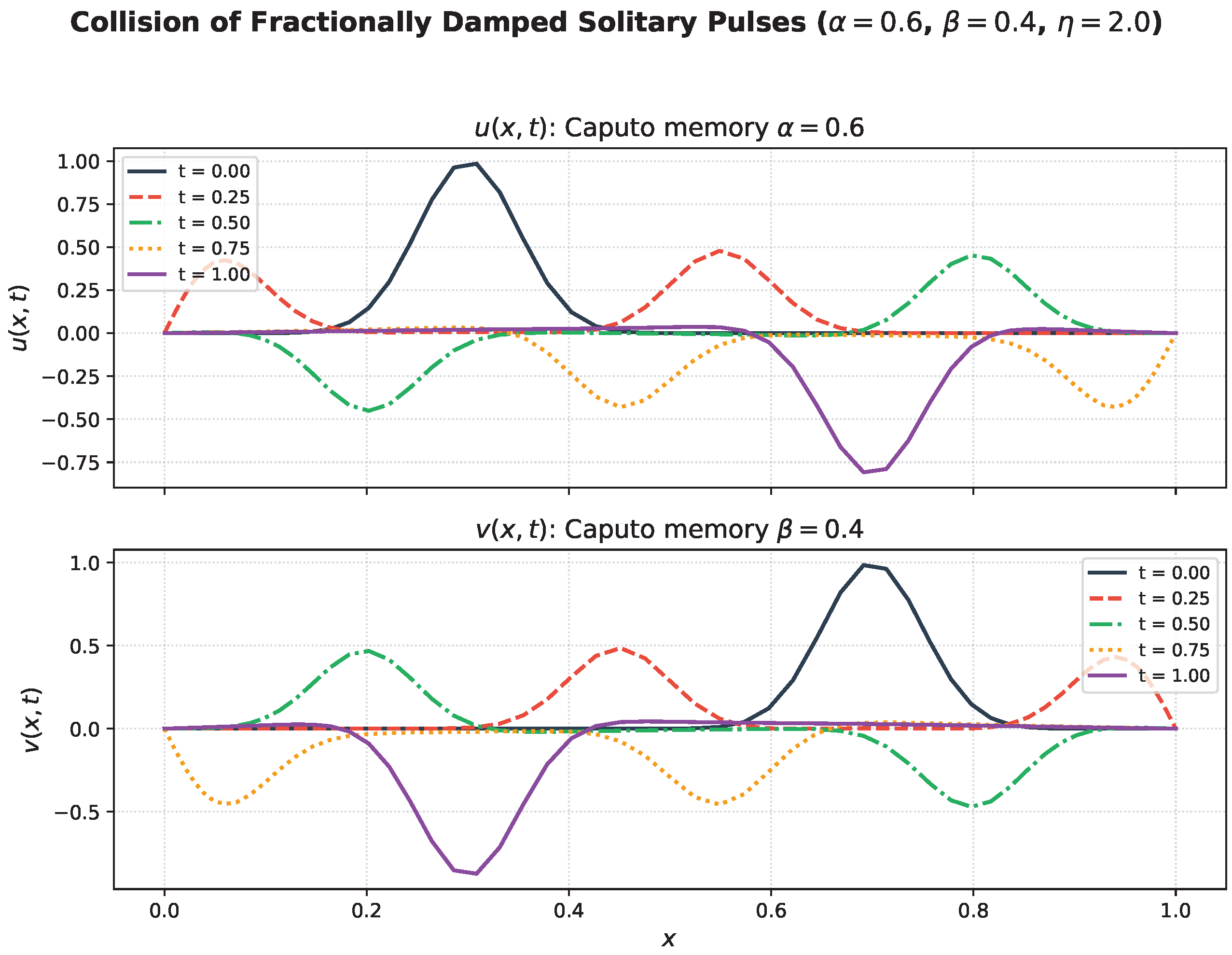
Table 1.
Comparison of the present method with existing approaches for fractional Klein–Gordon-type equations. KG = Klein–Gordon, KGS = Klein–Gordon–Schrödinger. “–” indicates the feature is absent.
Table 1.
Comparison of the present method with existing approaches for fractional Klein–Gordon-type equations. KG = Klein–Gordon, KGS = Klein–Gordon–Schrödinger. “–” indicates the feature is absent.
| Feature | [5] | [6] | [7] | [11] | [21] | [22] | Present |
|---|---|---|---|---|---|---|---|
| Equation type | scalar KG | scalar KG | scalar KG | scalar diff. | coupled KGS | coupled KGS | coupled KG–KG |
| Nonlinear () | – | ✓ | ✓ | – | ✓ | ✓ | ✓ |
| Spatial method | FDM | Cheb. | Leg. | FDM | FDM | Galerkin | Cheb. colloc. |
| Fractional type | time | time | time | time | space | space | time (Caputo) |
| Two distinct orders | – | – | – | – | – | – | ✓ () |
| SOE acceleration | – | – | – | ✓ | – | – | dual SOE |
| IMEX lineariz. | – | – | – | – | – | – | ✓ |
Disclaimer/Publisher’s Note: The statements, opinions and data contained in all publications are solely those of the individual author(s) and contributor(s) and not of MDPI and/or the editor(s). MDPI and/or the editor(s) disclaim responsibility for any injury to people or property resulting from any ideas, methods, instructions or products referred to in the content. |
© 2026 by the authors. Licensee MDPI, Basel, Switzerland. This article is an open access article distributed under the terms and conditions of the Creative Commons Attribution (CC BY) license (http://creativecommons.org/licenses/by/4.0/).
Copyright: This open access article is published under a Creative Commons CC BY 4.0 license, which permit the free download, distribution, and reuse, provided that the author and preprint are cited in any reuse.


