

Submitted:
23 July 2026
Posted:
23 July 2026
You are already at the latest version
Abstract
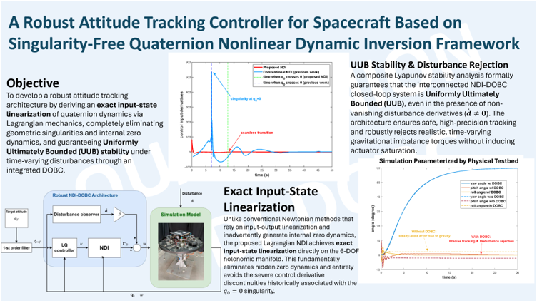
This paper presents a robust attitude-tracking control architecture for rigid spacecraft subject to model mismatches and external disturbances. Quaternions are utilized for attitude representation to prevent the gimbal lock associated with Euler angles. While conventional nonlinear dynamic inversion (NDI) relies on Newtonian mechanics and input-output linearization — which inadvertently generates internal zero dynamics and encounters severe control derivative discontinuities at the \( q_0 =0 \) singularity — this study proposes a novel NDI framework derived strictly from Udwadia’s Lagrangian formulation. This approach realizes an exact input-state linearization directly on the 6-degree-of-freedom active holonomic constraint manifold, completely eliminating internal zero dynamics and mathematical singularities. To ensure robustness against physical uncertainties, the singularity-free NDI is augmented with a nonlinear disturbance observer (DOBC) and an outer-loop linear-quadratic (LQ) tracking controller. A rigorous composite Lyapunov stability analysis is conducted for the complete closed-loop architecture. The analysis formally guarantees that both the isolated disturbance estimation error and the fully interconnected dual-loop NDI-DOBC system are Uniformly Ultimately Bounded (UUB), even in the presence of realistic, time-varying disturbances with non-vanishing derivatives (\( \dot{\textbf{d}}\neq \textbf{0} \)). Comprehensive numerical simulations, parameterized by a physical spherical air-bearing testbed subject to state-dependent gravitational imbalance torques, validate the architecture's exceptional tracking precision, smooth transient response, and robust disturbance rejection.
Keywords:
quaternions
; input-state linearization
; nonlinear dynamic inversion
; disturbance observer-based controller
; spacecraft attitude control
1. Introduction
The control of spacecraft attitude has evolved significantly, progressing from classical linear techniques to advanced nonlinear architectures capable of meeting the rigorous agility requirements of modern missions. Conventional Proportional-Integral-Derivative (PID) controllers have served as the industry standard due to their implementation simplicity and extensive flight heritage. While effective for set-point regulation, PID designs often struggle with the strong gyroscopic coupling encountered during rapid, large-angle maneuvers. Some researchers have proposed modified PID methods to increase robustness and overcome the phenomenon [1]. To address the multi-variable interactions, Linear Quadratic Regulator (LQR) was introduced, providing a systematic framework for minimizing energy and error for multi-input-multi-output (MIMO) systems [2,3,4,5]. However, both PID and LQR are inherently limited by their linearization around equilibrium points and often need extensive gain scheduling to cover the full flight envelope. To bridge this gap, Linear-Parameter-Varying (LPV) control has emerged as a powerful intermediate solution [6,7], allowing designers to embed nonlinear dynamics into a family of linear models scheduled by state-dependent parameters, thus extending the valid operating range of linear techniques.
Despite these advancements, the nonlinearity of rigid body dynamics - particularly at high angular velocities - has driven research toward purely nonlinear control paradigms. Sliding Mode Control (SMC) has been widely investigated for its robust properties, utilizing discontinuous control laws to force system states onto a predefined sliding manifold [8]. While SMC is theoretically invariant to matched uncertainties, it famously suffers from the “chattering” phenomenon, which can excite high-frequency structural modes and wear down actuators. Another way to address the nonlinearity is nonlinear dynamic inversion (NDI), also known as feedback linearization, which offers a more geometric and physically intuitive alternative. Unlike robust controllers that fight against nonlinearities, NDI exploits the system’s physics to cancel them. By algebraically transforming the nonlinear spacecraft dynamics into a linear time-invariant (LTI) system, NDI enables the application of well-understood linear control laws to the “synthetic” LTI system.
The NDI technique has been widely implemented in aerospace systems, from aircraft flight control [9,10], reentry vehicle [11], reusable rocket [12], and satellites [8,13,14]. A two-loop cascaded flight control architecture is commonly used for attitude control based on the assumption of time-scale separation. In this approach, the angular velocity loop (the inner loop) and the attitude loop (the outer loop) are linearized and controlled separately. This method simplifies the controller design process. Banerjee et al. [14] demonstrate the conventional two-loop structure NDI in the attitude control of a lunar lander, employing Euler angles for attitude representation. However, the use of Euler angles is hindered by a singularity at pitch angles of ±90 degrees, a phenomenon known as gimbal lock. As a result, alternative approaches for attitude representation, such as quaternions, have garnered increasing attention. Zhang et al. [15] design a quaternion-based NDI for fixed-wing UAV flight controller, but still using the conventional two-loop structure.
Unlike the conventional cascaded structure, we can select quaternions as the output and directly linearize them with respect to the input torque using the NDI technique. The angular velocity is implicitly dictated by the quaternion kinematics equation [8]. However, there is a dimension mismatch between the output quaternion, which is represented as a vector in , and the input torque, which is a vector in . To resolve this issue, previous studies [8,13,16,17] have used only the vector part of the quaternions as the output, while computing the scalar part using the unit-quaternion constraint. It has been noted, however, that a singularity may occur in the matrix inversion during NDI when the scalar part of the quaternions is zero, leading to numerical instability in control processes. Long et al. [16] and Navabi et al. [17] demonstrate that the internal dynamics of the linearized system remain stable as long as the scalar part of the quaternions is non-zero. To address this issue, Bang et al. [8] proposed adding a small value to the scalar part of the quaternions when it approaches zero, thus avoiding singularities. Bhargavapuri et al. [18] focused on quaternion error, defined as the difference between the desired and actual quaternions. They integrated the scalar part of the quaternions into the NDI framework to prevent it from crossing zero.
The NDI can effectively cancel system nonlinearity, but its performance relies heavily on the accuracy of state feedback and the model information. Model discrepancies and external disturbances can impair the effectiveness of the nonlinearity cancellation. To mitigate the sensitivity of conventional exact linearization to model mismatch, recent literature has heavily favored Incremental Nonlinear Dynamic Inversion (INDI) [19,20]. While INDI successfully bypasses deep model dependencies, it strictly requires high-fidelity angular acceleration measurements. In practical attitude control architectures, differentiating noisy IMU signals severely amplifies high-frequency noise, risking actuator saturation. Therefore, returning to an exact, model-based NDI approach augmented with an active disturbance observer remains practically superior for environments where sensor noise is prevalent.
Chen and Yang [21,22] introduced a nonlinear disturbance observer-based control (DOBC) approach to improve the NDI’s ability to manage disturbances and uncertainties resulting from model mismatches. The DOBC consists of two main components: disturbance estimation and compensation. Chen et al. [23] categorized various types of observers based on their application to linear or nonlinear systems, as well as the compensation mechanisms addressing external disturbances or model mismatches.
Consequently, DOBC and Extended State observers (ESO) have seen continued advancement for robust spacecraft and UAV tracking applications [15,24]. These state-of-the-art observer designs provide excellent lumped disturbance rejection. However, integrating these modern observers with quaternion-based NDI presents a distinct challenge. Conventional input-output linearization on the quaternion vector part often induces unwinding or unstable internal zero dynamics, compromising the observer’s stability guarantees.
Previous research indicates that matrix inversion in NDI is related to the control input and the second derivatives of the output function in rotational dynamics. While earlier studies employed Newtonian mechanics to describe these motions, they encountered singularities with the matrix inverse. Therefore, it is worthwhile to explore alternative approaches. Udwadia et al. [25] present a direct method for obtaining Lagrange rotational motion using quaternions. This approach establishes the relationship between torque and the second derivatives of quaternions, while accounting for the unit-quaternion constraints.
In this paper, we derive a quaternion-based NDI using the Lagrange equation of motion, not suffering from the singularity issues observed in previous studies. Crucially, unlike conventional Newtonian approaches that rely on input-output linearization and inadvertently generate internal zero dynamics, our pure Lagrangian derivation achieves an exact input-state linearization. Because the synthetic linear states are chosen to be mathematically identical to the Lagrangian physical states, the required state coordinate transformation constitutes a perfect global identity diffeomorphism. Furthermore, we rigorously prove the complete realization of this LTI framework. By deriving a structurally non-singular input-transformation and satisfying the necessary differential geometry conditions – specifically, proving that the input distribution is inherently involutive and strictly spans the active constraint manifold – we guarantee that the exact input-state linearization is completely realized on the 6-degree-of-freedom holonomic manifold without inducing any hidden zero dynamics.
After eliminating the nonlinearity using NDI, we can implement a linear controller for the input-output linearized system. In this paper, we design a Linear Quadratic Tracking (LQ) controller that incorporates both feedback and feedforward gains to achieve the desired attitude while ensuring the stabilization of the quaternions and their derivatives. Additionally, a first-order filter is introduced before the controller to smooth the reference signal, rather than applying a step signal directly. This approach helps prevent actuator saturation.
To guarantee robustness against exogenous disturbances, we augment the NDI framework with a DOBC. By designing the nonlinear observer gain to respect the geometric properties of the quaternion, we formally prove that the disturbance estimation error is uniformly ultimately bounded (UUB), even in the presence of a non-vanishing disturbance derivative (. Furthermore, rather than analyzing the observer and controller in isolation, we construct a composite Lyapunov function to evaluate the complete NDI-DOBC interconnected system. This rigorous stability analysis demonstrates that the total close-loop system remains strictly UUB, mathematically ensuring safe and robust tracking performance without compromising the strictly separated observer-controller software architecture.
Finally, to validate these theoretical contributions, comprehensive numerical simulations are conducted to evaluate the proposed architecture against conventional input-output linearization methods. The comparative analysis explicitly demonstrates that the proposed exact input-state linearization successfully eliminates the discontinuity in the control input derivative at the quaternion singularity (), ensuring smooth and physically realizable control efforts during large-angle, shortest-path maneuvers. Furthermore, the simulations are grounded in the physical parameters of an actual spherical air-bearing attitude control testbed. By explicitly modeling the realistic, time-varying external disturbance torque induced by the gravitational imbalance – resulting from the inevitable misalignment between the center of gravity and the center of rotation – we demonstrate that the proposed NDI-DOBC framework achieves exceptional robust tracking performance, fully validating the theoretical UUB stability guarantees.
In summary, the main contributions of this paper are outlined as follows:
- Exact input-state linearization via Lagrangian mechanics: Unlike conventional Newtonian approaches that utilize input-output linearization and inadvertently generate internal zero dynamics, this work derives a quaternion-based NDI strictly utilizing the Udwadia formulation. This achieves an exact input-state linearization on the 6-degree-of-freedom holonomic manifold, eliminating zero dynamics and avoiding the control input derivative discontinuities typically found at singularity.
- Disturbance observer design: To address dynamic external disturbances, a nonlinear disturbance observer is designed. By selecting an appropriate observer gain that respects the geometric properties of the quaternion, we mathematically prove that the disturbance estimation error is Uniformly Ultimately Bounded (UUB), even in the presence of a non-vanishing disturbance derivative ().
- Interconnected closed-loop stability proof: Moving beyond isolated observer and controller analysis, a composite Lyapunov function is constructed to evaluate the complete NDI-DOBC architecture. This stability analysis formally guarantees that the interconnected system remains strictly UUB, mathematically validating the separated controller-observer framework.
- Physical testbed simulation and validation: The theoretical framework is validated through comprehensive numerical simulations parameterized by the physical properties of a spherical air-bearing attitude control testbed. The results demonstrate the proposed method’s superiority over the conventional approaches, showcasing exceptional tracking robustness against realistic, time-varying gravitational imbalance torques.
2. System Architecture
This section introduces the schematic of the NDI-DOBC architecture and the attitude control testbed. First, we present a system overview in the form of a block diagram, providing a visual summary of the framework.
2.1. System Block Diagram
The NDI-DOBC block diagram is shown in Figure 1. For clarity, we delineate the signal propagation from the reference input to the system output. The design process is divided into signal filtering, linear quadratic (LQ) tracking control, nonlinear-dynamic-inversion (NDI) linearization, and disturbance observation. This graphical mapping connects the general overview to each subsystem described below.
A first-order filter, acting as a signal smoother, is placed before the controller to smooth the input signal. For a large-angle maneuver, this smoother outputs a continuous curve to the controller instead of a step function. This prevents excitation of the nonlinearity and actuator saturation from rapid movement. The linear-quadratic tracking controller is designed using the linearized system. It stabilizes the system with state-feedback gains and provides feed-forward gains to improve tracking accuracy. The outputs of the LQ tracking controller, known as “virtual inputs,” serve as the inputs to the linearized system. The NDI then converts these “virtual inputs” into real, physically meaningful control torques for rotational motion.
The disturbance observer, shown as an orange block, estimates external disturbance using information from the original nonlinear system. The nonlinear function and the observer gain are to be designed to ensure the disturbance estimate error stays asymptotically stable regardless of the states . The estimated disturbance is then multiplied by the compensation gain and added to the NDI control torques. These serve as inputs to the nonlinear system. Details are given in Section IV.
2.2. Physical Disturbance Modeling and Theoretical Bounds
The primary exogenous disturbance acting on the attitude testbed arises from physical misalignment between the system’s center of gravity (CG) and its center of rotation, as illustrated in Figure 2. Let denote the position vector of the CG relative to the center of rotation, and represent the total mass of the testbed. The resulting gravitational imbalance torque, , is formulated as:
Where represents the local gravitational acceleration vector. Because the direction of relative to the inertial gravity vector changes continuously as the testbed rotates, this disturbance torque is inherently state-dependent and time-varying.
However, because the testbed is mounted on a spherical air-bearing, its maximum tilt angle is strictly constrained by the physical limits of the mechanical structure. Consequently, the magnitude of the gravitational imbalance torque is fundamentally upper bounded by an absolute physical maximum, yielding the inequality . Furthermore, since the angular velocity of the system is physically constrained by the finite saturation limits of the control actuators, the time derivative of the disturbance torque is mathematically guaranteed to be strictly bounded, satisfying .
3. Quaternion Rotation Dynamics
This section introduces the Lagrange equation of rotational motion using quaternions, which is essential for deriving NDI in the next section. Udwadia first derived this equation in 2010 using a direct Lagrange approach without relying on the concept of Lagrange multipliers or Newtonian mechanics [25]. The derivation constructs the Lagrangian from energy terms and expresses the unconstrained equation of motion in terms of quaternions, their derivatives, angular velocity, and generalized torque. The unit-quaternion constraint is incorporated by applying the fundamental equation of constrained motion [26], resulting in a constrained equation of motion. The relationship between generalized and physical torque is then established, providing an equation that describes rotational dynamics in terms of quaternions while satisfying the unit-quaternion constraint for a given input torque.
The derivation begins with the Lagrangian, defined as kinetic energy minus potential energy. For rotational motion, only kinetic energy is present, so the Lagrangian is . The body-fixed coordinate axes are assumed to align with the principal axes of the rigid body, resulting in a diagonal moment of inertia matrix . The Lagrange equation of motion is:
Equation (2) is an unconstrained equation of motion. The quaternion vector serves as the generalized coordinate, with each element considered independent. Quaternions are divided into the scalar part and the vector part . The input to Equation (2) is a generalized quaternion torque vector . Several properties of quaternions are useful for expanding and rearranging Equation (2):
Quaternion time derivatives: The quaternion time derivative is defined as the “quaternion product” of the quaternion and the augmented angular velocity:
Here, denotes the quaternion product, and the augmented angular velocity is . Using the properties of quaternions, Equation (3) can be rearranged into two matrix forms [27]:
and represent the orthogonal matrix of quaternions and its time derivative:
From Equation (4), the augmented angular velocity can be expressed as:
Properties of matrix and : is a submatrix of shown in Equation (5). is an orthogonal matrix, and is a matrix with orthogonal rows, hence they have the following property:
lies in its null space because each row of is orthogonal to . Multiplying by the quaternion vector yields a zero vector:
From Equations (5) and (8), it follows that:
Substituting the quaternions with their time derivatives in Equation (8), the matrix transforms into . Each row of is orthogonal to :
Equation (10) will appear later for the observer gain design.
Unit-quaternion constraint: When quaternions represent attitude, they must satisfy the unit-norm constraint: . This leads to the following expression:
Differentiate Equation (9) with respect to time, and substitute the result into Equation (6), this yields another expression of augmented angular velocity:
Substituting Equations (6) and (12) into the kinetic energy equation, the rotational kinetic energy can be expressed in terms of quaternions and their derivatives:
is a moment of inertia matrix, and is a extended moment of inertia matrix matching the dimension of , where is an arbitrary positive number. The unconstrained Lagrange equation of motion (2) can also be rearranged as follows:
Applying the fundamental equation of constrained motion [26] incorporates the unit-quaternion constraint into the unconstrained system. After algebraic manipulation, the arbitrary number is eliminated, and the generalized acceleration is given by Equation (14) as
in Equation (15) denotes the skew-symmetric matrix of angular velocity, defined as:
For practical applications, the generalized quaternion torque vector must be converted to a physical torque . Udwadia [25] established the relationship between these torques using the “virtual work method,” resulting in:
By substituting Equation (17) into Equation (15), the Lagrange equation of motion for rigid body rotation using quaternions and body-fixed frame torque is obtained:
4. Quaternion NDI and LQ Tracking Controller
In this section, we apply nonlinear dynamic inversion (NDI) to the rotational dynamics – based on the Lagrange equations of motion presented in Equation (18) – to obtain a linearized dynamic model. Following this, a linear quadratic (LQ) tracking controller is developed for the linearized system, utilizing both state feedback and feedforward gains to ensure precise tracking performance.
To simplify controller design, we apply exact input-state linearization to transform the nonlinear rotational dynamics into synthetic Linear Time-Invariant (LTI) system. By comparing the system equations with the Lagrange equation of motion from Section 3, we define the complete system state vector using the quaternions and their time derivatives, .
Equations (4) and (18) can be rewritten as follows:
where the drift vector field and the input matrix are partitioned as:
Here, the angular velocity vector is treated as a parameter, with its relationship to given in Equation (4). If the quaternion time derivatives are bounded, the angular velocity will also remain bounded.
The control inputs are the torques applied to the body axes, . To perform the input-state linearization, we examine the lower partition of the state equations, which governs the angular acceleration ():
By defining the second derivative of the quaternions as the “virtual input”, , we can algebraically cancel the system nonlinearities. Let and . The acceleration dynamics become:
Utilizing the Moore-Penrose pseudoinverse of the decoupling matrix , we derive the input transformation mapping the virtual control to the physical torque :
Expanding the Equation (23) yields:
Since is not a square matrix, we use the pseudoinverse of . In the next subsection, we examine whether a singularity exists in this NDI formulation, as observed in previous studies [13,16,17,18].
Finally, the linearization system is shown below:
where is the states vector and is the input vector of the LTI system.
4.1. Singularity Analysis of the Matrix Inversion
The matrix in Equation (24) is a matrix. To determine whether a pseudoinverse exists, we examine its column rank. If the rank is 3, the pseudoinverse exists, and no singularity occurs during inversion. To show that is full column rank, it is equivalent showing that the matrix is full rank and invertible.
Since the result in equation (26) is a diagonal matrix and the moments of inertia of the principal axes are always positive, is full column rank and its pseudoinverse exists.
The pseudoinverse of is referred to as a “left inverse” because it is a tall matrix. The inverse is provided below:
In previous works [16,17] that derive the NDI formulation using a Newtonian mechanics approach, the counterpart matrix to be inverted has the form:
With its determinant
The result shows a singularity at , which leads to numerical instability when calculating the control torque.
In summary, the NDI formulation derived from the Lagrange mechanics approach can include both the vector and scalar parts of quaternions as outputs. Importantly, this approach does not exhibit the singularity reported in previous work, providing a robust foundation for controller design.
4.2. Proof of Exact Input-State Linearization
To formally establish that the proposed Lagrangian NDI constitutes an exact input-state linearization rather than a conventional input-output linearization, the geometric condition of the state transformation must be rigorously verified. In standard Newtonian formulations, linearizing the rotational dynamics typically involves selecting the vector part of the quaternion as the system output. This approach dictates a coordinate transformation that inevitably splits the state space, leaving the scalar part of the quaternion as internal zero dynamics.
Conversely, the Udwadia formulation operates directly on the generalized coordinates while intrinsically preserving the holonomic constraint () without requiring state partitioning. Because the Lagrangian derivation comprehensively maps the physical constraints into system’s kinetic energy, the nonlinear coordinate transformation required to map the original dynamics into the synthetic LTI space is simply the identity mapping:
For exact input-state linearization to be theoretically valid, the coordinate transformation must be a diffeomorphism. The Jacobian matrix of the proposed transformation evaluates trivially to the identity matrix:
Since the identity matrix is globally non-singular and its inverse is smooth, the mapping constitutes a global diffeomorphism. This mathematical property is highly significant: it guarantees that the entire mathematical state vector is seamlessly and invertibly mapped into the synthetic linear domain. Consequently, the entire state space is fully observable and controllable within the linear framework, rigorously proving the complete absence of internal zero dynamics.
With the global diffeomorphism established, the second requirement for input-state linearization is a well-defined, non-singular input mapping. As derived in the beginning of Section 4, the algebraic mapping between the virtual control input and the physical torque is given by . Because the decoupling matrix is analytically proven to maintain full column rank across the entire operational manifold, its pseudoinverse is globally well-defined. Therefore, this input transformation strictly guarantees the exact algebraic cancellation of the nonlinear dynamics without encountering the mathematical singularities inherent to conventional Newtonian formulations.
Finally, to eliminate any theoretical ambiguity regarding the realization of this LTI system, the proposed transformation must satisfy the necessary and sufficient differential geometry conditions established by the Frobenius Theorem [28]. Let the system input matrix be partitioned into its three constituent column vector fields, such that , where each corresponds to a distinct control input channel. For the feedback linearization of our system, the input distribution is defined by the span of these column vector fields:
For exact linearization to be mathematically realized, this distribution must be involutive. Because the input vector fields are structurally independent of the angular velocities , the Jacobian cross-multiplications strictly evaluate to zero. Consequently, the Lie brackets of any two input vector fields commute and vanish (), proving is completely involutive.
Furthermore, to evaluate the multi-input-multi-output exact linearization, the “controllability-like” block matrix must be constructed using the Lie brackets between the drift vector field and the input distribution. Because the physical control inputs are torques acting on rotational dynamics, the relative degree of each input channel to the attitude state is for . According to feedback linearization theory, the maximum order of the required Lie brackets in matrix is . Thus the required block matrix is formulated as:
Let define the unconstrained domain of the mathematical vector . In conventional unconstrained systems, exact linearization would require to have a rank of 8. However, governed by the Udwadia formulation, the system’s actual physical trajectories are permanently restricted to the active holonomic constraint manifold defined by and . Let this 6-degree-of-freedom constraint manifold be defined as the specific operational subdomain .
As established by the full column rank of the decoupling matrix , the block matrix strictly possesses a rank of 6 for all . Because the sum of the relative degrees () precisely equals the topological dimension of the active manifold , the exact full input-state linearization is completely realized on this constraint manifold. This rigorously proves that within the physically valid domain , the transformation achieves perfect LTI realization without generating any internal zero dynamics.
4.3. Linear Quadratic Tracking Controller
After the NDI formulation, a linear quadratic controller is designed to determine the virtual input in Equation (25). In Figure 1, the blue area represents the linearized equivalent system, and the LQ controller provides the virtual input to control the linearized state and track the reference signal .
A linear quadratic controller for attitude tracking is formulated to minimize the cost functional:
and subject to the linearized dynamic system (25). and are positive definite matrices representing the weighting matrices for the linear system’s states and virtual inputs. The control input vector computed by the linear quadratic method takes the form: , where is the state feedback gain and is the feedforward term [29].
The state feedback gain is obtained by solving the Riccati equation. In our case, it can be partitioned into two submatrices, , corresponding to their respective state variables. When tracking a desired attitude, , we set the desired state vector as , and the 1st-order filter generates smooth sequence of equilibrium points as reference signal for the controller instead of a step signal. The feedforward term is then . To summarize, the virtual control input consists of both feedback and feedforward components, as shown below.
5. Nonlinear Disturbance Observer-Based Controller
Nonlinear systems often encounter unmodeled disturbances, which can significantly impact the performance of model-based controllers. These disturbances may originate from the external environment, parameter uncertainty, or unmodeled dynamics. Chen et al. [23] classified such disturbances as either matched or mismatched. In our application, external disturbances result from shifts in the center of gravity and the center of the spherical air-bearing, producing additional torque on the attitude control testbed. Because this disturbance acts through the same channel as the control torque, it is considered as a matched disturbance. The rotation dynamics with external disturbances can be represented as follows:
The state vector, , matches the nonlinear system in equation (19). corresponds to the matrix in equation (20), while maps disturbances into the state space. For matched disturbances, we have .
In the DOBC framework, the controller and disturbance observer loops are designed independently. This separation principle enables the direct application of the NDI and LQ controller results from the previous section. We first introduce the DOBC framework to propose a nonlinear observer gain function based on the Lagrange equation of motion using quaternions, and then combine the control torque from the LQ controller with the estimated disturbance to obtain the final control inputs for the nonlinear system (38). The orange block in Figure 1 illustrates the disturbance observer structure. The estimated disturbance is fed forward to the control input through the triangular gain block , located between the blue and orange blocks.
Chen et al. [23] reviewed various disturbance observers and their corresponding DOBCs, considering the characteristics of the target system and disturbances. For nonlinear systems with matched disturbances, they propose a nonlinear disturbance observer:
The observer output, in the lower part of Equation (37), represents the estimated disturbance. It is calculated as the sum of the observer’s internal states, , and a nonlinear function, , which must be designed. The upper part of Equation (37) describes the dynamics of the internal states, which depend on the nonlinear system (38). The relationship between observer gain function and is given below:
The observer gain function is synthesized based on the nominal disturbance assumption (). Under this condition, the nominal disturbance estimation error dynamics are defined as:
Equation (39) is a first-order ODE. If the designed gain ensures that is positive definite, the nominal error dynamics are asymptotically stable. The disturbance estimation error is defined as the difference between the actual disturbance and its estimate, . Therefore, when designing the disturbance observer, we first determine , then obtain by integrating . The following subsection discusses the details of designing the observer gain function.
Equation (39) is a first-order ODE. If is positive definite, the ODE is stable. The gain function can be defined as , so . Since , and , equation (39) is equivalent to:
Therefore, we can design first by setting . To guarantee that be positive definite, we can simply let it be an identity matrix multiplied by a positive-scalar gain . Learning that , and the property in Equation (7),we can set so that
It is clear from Equation (38) that is the partial derivative of with respect to . Expanding yields:
The nonlinear function can be obtained by integrating with respect to . Assuming a zero constant of integration for simplicity, which leads to:
And can be derived by partially differentiating with respect to .
While the condition does not affect Equation (39) and allows us to design first, the dynamics in Equation (37) includes the term . Since , it is necessary to investigate the influence of on . From the property described by Equation (10), it follows that:
Given that has no influence on the dynamics of , as shown in Equation (47), the gain becomes negligible. Thus, the observer gain function is constructed as:
After determining and , the estimated disturbance can be obtained from Equation (37). The system input should not be taken directly from the control torque calculated by the NDI and LQ controller. Disturbance compensation is applied before the control torque is used in the nonlinear system:
The in the equation above is the disturbance compensation gain. Chen et al. [23] provided various methods for determining this gain. In the case of matched disturbances, where , the gain reduces to -1. Therefore, the control input for the nonlinear system becomes:
5.1. Lyapunov Stability Analysis of the Disturbance Observer
Having established the observer gain matrix to stabilize the nominal system, we now evaluate the actual disturbance estimation error in the presence of physical, time-varying disturbances. In reality, the gravitational imbalance torque possesses a non-vanishing derivative (). Therefore, the true error dynamics are governed by:
Consider the following positive-definite Lyapunov candidate function for the observer error dynamics:
Taking the time derivative of along the trajectories of the error dynamic yields:
Substituting the derived relation , the derivative becomes:
Utilizing the Rayleigh quotient and the Cauchy-Schwarz inequality, we can bound the Lyapunov derivative as follows:
As established in Section 2.2, the time derivative of the gravitational imbalance disturbance is strictly bounded by . Applying this physical bound:
For the Lyapunov derivative to be strictly negative (), the norm of the estimation error must satisfy:
This result mathematically guarantees that the disturbance estimation error is Uniformly Ultimately Bounded (UUB). The error will converge exponentially to an ultimate bound defined by , and remain within this bounded region thereafter.
The theoretical bound reveals a critical engineering design trade-off. While mathematically minimizing this bound requires maximizing the convergence speed via a very large observer gain, doing so practically risks amplifying unmodeled high-frequency noise and inducing undesirable transient behaviors. Prioritizing system stability and smooth transitions dictates the selection of a more moderate gain. The specific numerical selection of this gain, alongside a comprehensive analysis of its impact on the transient behavior, is detailed in the simulation results presented in Section 7.
6. Stability Analysis of the Interconnected NDI-DOBC System
To guarantee the robustness of the complete attitude control architecture, it is imperative to analyze the coupled stability of the linear quadratic tracking controller and the nonlinear disturbance observer. While the previous sections established the stability of each subsystem in isolation, the estimated disturbance introduces a cross-coupling effect into the closed-loop tracking dynamics must be bounded.
6.1. Perturbed Tracking Error Dynamics
Let the state tracking error of the linearized system be defined as . Without environment disturbances, the closed-loop LTI dynamics under the state-feedback LQ controller are governed by , where is a Hurwitz system matrix.
However, under the influence of the physical disturbance and the composite control law , the input transformation is purturbed by the disturbance estimation error, . Consequently, the closed-loop tracking error dynamics are formulated as:
Where is the linear input matrix mapping the virtual acceleration.
6.2. Composite Lyapunov Function and Stability Proof
To evaluate the interconnected system, we construct a composite Lyapunov candidate function. A weighting constant is introduced to scale the observer’s estimation error dynamics:
For the LTI tracking system, because is Hurwitz, for any given symmetric positive-definite matrix , there exists a unique symmetric positive-definite matrix that satisfies the continuous-time Lyapunov equation:
Taking the time derivative of along the system trajectories yield:
Substituting Equation (56) and the observer error dynamics () results in:
Applying Equation (58) and utilizing the Rayleigh quotient, the first term on the right-hand side, the nominal tracking term, is bounded by the minimum eigenvalue of :
To separate the cross-coupling term , we apply Young’s inequality. For any vectors and any strict positive scalar , the inequality states .
Let and :
Substituting these bounds into Equation (60) and applying the physical disturbance bound , we obtain:
Rearranging the terms to group the state norms:
For the interconnected system to maintain bounded stability, the coefficients of the quadratic error terms must be strictly positive. This establishes two critical design conditions that govern the selection of the Young’s inequality scaling parameter , the Lyapunov weighting constant , and the observer gain :
By first selecting a sufficiently large to satisfy the first condition, we can subsequently define a weighting constant and an observer gain that satisfy the second condition. With these parameters established, let the strictly positive constants be defined as and .
The Lyapunov derivative simplifies to:
Rearranging Equation (66) yields:
For the overall Lyapunov derivative to be strictly negative (), it is sufficient that the norm of the disturbance estimation error satisfies:
Since is always semi-negative, whenever this condition holds, is negative definite outside a bounded compact set.
This mathematical inequality rigorously guarantees that the complete interconnected NDI-DOBC system is Uniformly Ultimately Bounded (UUB). The state tracking error and the disturbance estimation error will concurrently converge to a compact region bounded by the physical limits of the testbed’s disturbance derivative (). Once the errors converge into this boundary, they will remain there indefinitely, formally proving the robust tracking stability of the proposed dual-loop architecture.
7. Simulation Results
This section presents the simulation results utilized to validate the efficacy of the proposed NDI-DOBC methodology. We categorize the simulations into four cases. First, the attitude tracking control with the zero-crossing of the scalar component of quaternion () is examined under ideal conditions, characterized by a diagonal moment of inertia matrix and the absence of external disturbance. To underscore the singular-free attributes of the proposed NDI framework, we adopt the moment of inertia matrix and initial, final conditions from previous work [8] and compare the simulation results. In the subsequent case, we adjust the moment of inertia matrix and add off-diagonal elements to test the robustness of the linear quadratic tracking controller in cooperation with the NDI framework.
Before detailing the specific simulation cases, the physical parameters of the attitude control testbed – which define the theoretical disturbance bounds established in Section 2.2 – are quantified. The modeled testbed has a total mass of 19.899 kg and a center of gravity (CG) displacement of [0.02, 0.02, 0.05] m from the center of the spherical air-bearing. Evaluated under standard local gravitational acceleration, this yields an absolute maximum gravitational imbalance torque bound of . Furthermore, the physical control torque saturation limit of the actuator is strictly set to 5.25 . Constrained by this maximum control effort and the resulting rotational dynamics, the maximum allowable rate of change of the disturbance torque is calculated and bounded by .
The first case focuses on the general spacecraft static-to-static attitude control scenario, where the initial and target attitudes are denoted by and , respectively. To further demonstrate the performance optimization capabilities of the proposed architecture, Case 1 also includes an additional comparative result utilizing a smaller system time constant. This specific tuning is designed to significantly accelerate the convergence rate while remaining strictly within the physical control saturation limits, highlighting an optimal balance between aggressive tracking and actuator constraints.
In contrast, the second case considers a dynamic transition from an initially rotating state with an angular velocity of to a static target attitude . The moment of inertia matrices for simulation Case 1 and 2 are defined as follows. In Case 1, a purely diagonal moment of inertia matrix, , is used for both the derivation of the NDI control law and the plant simulation. In case 2, is retained for the NDI controller derivation to introduce a deliberate model mismatch, while the actual plant simulation is conducted using the full matrices featuring off-diagonal coupled inertias (, and ):
The third simulation case introduces external disturbances, focusing on the attitude control testbed as the physical target. As illustrated in Figure 2, the disturbance is induced by the misalignment between the testbed’s center of gravity and the support center of the air bearing, generating a state-dependent gravitational moment. The proposed DOBC is utilized to estimate and dynamically counteract this specific disturbance impact. Given the constrained roll and pitch angles of the physical testbed, new operational initial and target conditions are defined. Represented in Euler angles, the testbed transitions from an initial roll, pitch, and yaw of -5°, 10°, and 0° to a final target of 0°, 0°, and 60°.
The fourth case considers the simultaneous presence of both model mismatch and external disturbance, reflecting the realistic scenario of the attitude control testbed. The true moment of inertia of the testbed, , is calculated using CAD software and applied as the plant baseline in simulation Cases 3 and 4. To test the framework’s robustness, the NDI control law is deliberately handicapped by only being supplied with the diagonal elements of .
7.1. Case 1: Zero Crossing of Quaternions
The simulation of quaternions is shown in Figure 3. The results are compared with those from Bang’s work [8], which utilizes a conventional linear controller alongside Newtonian NDI. The scalar component of quaternion, , crosses zero at approximately t=12.7 seconds in our simulation, indicated by the green dashed line; In Bang’s case, this crossing occurs at t=7.9 seconds, marked by the blue dashed line. We can see that Bang’s controller experiences significant oscillations before reaching the desired attitude, whereas the proposed method yields a remarkably smooth convergence.
The most significant difference between the two controllers lies in the derivatives of the control input, as shown in Figure 4. Because Bang’s controller relies on an input-output linearization that possesses a mathematical singularity at , the system experiences severe numerical instability. This singularity causes massive, rapid fluctuations in the control input, with the derivative exceeding 500 , even with their proposed modified gain intended to mitigate the singularity. In contrast, the change in the control input for the proposed Lagrangian NDI remains completely smooth and bounded throughout the exact moment crosses zero.
To further demonstrate the tuning flexibility of the proposed LQ controller and the robustness of the singularity-free NDI framework, an additional simulation is conducted with a reduced system time constant (). The quaternion trajectories and the corresponding control input derivative for the aggressive tuning are presented in Figure 5 and Figure 6, respectively. As depicted in Figure 5, decreasing the time constant significantly accelerates the system’s convergence rate, allowing the spacecraft to reach the target attitude much faster than the nominal case.
However, as confirmed by the control input derivatives in Figure 6, the proposed architecture successfully accommodates the accelerated tracking without numerical failure. It is important to clarify the distinct roles of the control architecture components: while actuator saturation is prevented by the integrated first-order filter, the fundamental contribution of the proposed NDI is the complete elimination of the mid-maneuver control derivative peak. As seen in Figure 6, the control input derivative remains entirely smooth and continuous as crosses zero, proving that the Lagrangian formulation is fundamentally free from mathematical singularities regardless of the desired convergence speed.
Furthermore, an initial peak in the control input derivative – reaching approximately 400 – is observable at in Figure 6. This is a standard start-up transient caused by the instantaneous step in the commanded control torque from a zero initial state. Because the reduced time constant dictates a more aggressive initial angular acceleration, this start-up derivative is naturally larger than the case presented in Figure 4. Crucially, this initial transient is an expected physical response, completely distinct from the mathematically induced singularity spike that plagues conventional methods during the transient tracking phase.
7.2. Case 2: Robustness to Mismatched Moment of Inertia
In this case, we use the moment of inertia matrices , , and shown in Equation (69) for numerical simulation, but still adopt for deriving the NDI formulation. The cross-coupling terms and the decreasing diagonal terms in the moment of inertia matrices simulate the misalignment between principal axes and body-fixed axes and decreasing mass. The spacecraft is controlled by the LQ controller defined in Equation (34) with the weighting matrices and .
According to Newtonian rotational dynamics, the moment of inertia predominantly governs a system’s transient rotational behavior. Consequently, to explicitly evaluate this effect, Case 2 – unlike Case 1 – is initialized with a non-zero angular velocity. As illustrated in Figure 7, although variations in the moment of inertia yield distinct transient paths, all trajectories successfully converge to the reference quaternions. These results effectively demonstrate the robustness of the combined NDI and LQ control scheme in handling model mismatches.
7.3. Case 3: Robustness to External Disturbances
We introduce the DOBC derived in Section 5 to compensate for the influence of disturbances. The disturbance observer gain, , is tested with values of 1, 5, 10, and 20. Figure 8 shows the disturbance estimation error for the observer with different gains. Since the disturbances are related to the testbed’s attitude, we use the error between the disturbance and the estimated one as the performance index for the observer. Figure 8 indicates that the larger the observer gain, the faster the estimation error converges.
Figure 9 and Figure 10 also show that the observer gain will significantly influence the performance of attitude control. It appears that all the estimation errors converge to zero in Figure 8, but biases still exist at the steady state. Take y-axis for example, the value of equals 1 (green line) and 20 (red line) are in the order of magnitude of and . These biases cause the poor performance of the green line in Figure 9 and Figure 10.
Although the red lines () have the fastest convergence time, this large gain not only induces oscillations in disturbance estimation but also affects attitude control. Therefore, we select as the observer gain for implementation.
7.4. Case 4: Attitude Control with Both Model Mismatch and Disturbance
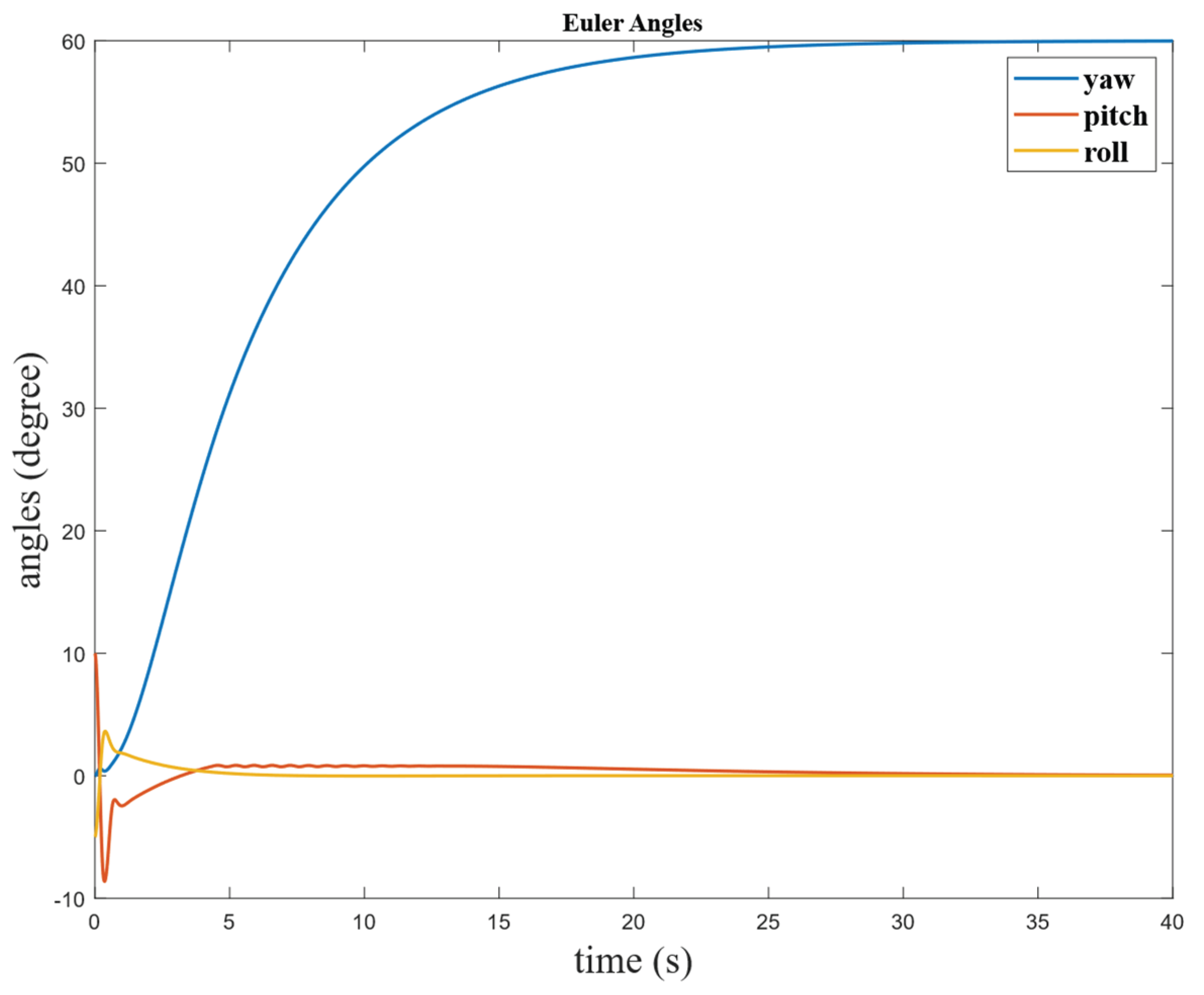
Finally, we adopt controller and observer gains designed from the two cases above and implement them in the scenario that contains both model mismatch and disturbance. The result is shown in Figure 11, where the yaw angle smoothly aligns with the desired heading. Meanwhile, the pitch and roll axes struggle to compensate for the disturbances caused by the initial pitch and roll angles. However, the DOBC rapidly takes effect to suppress these perturbations. Consequently, both axes achieve a smooth convergence to zero, while the yaw axis perfectly tracks the 60° target.
8. Conclusion
This paper presents a robust, singularity-free attitude tracking architecture for spacecraft, integrating a novel quaternion-based nonlinear dynamic inversion (NDI) framework with a disturbance observer-based controller (DOBC). By deriving the rotational dynamics strictly through Udwadia’s Lagrangian formulation, the proposed NDI achieves exact input-state linearization directly on the active holonomic constraint manifold. The geometric realization of this state transformation is mathematically proven to eliminate internal zero dynamics and entirely avoid the severe control derivative discontinuities historically associated with the singularity. To ensure robust performance against physical model uncertainties and time-varying environmental disturbances, a nonlinear DOBC is synthesized to augment a baseline linear quadratic (LQ) tracking controller. Rigorous Lyapunov stability analysis formally guarantee that both the isolated disturbance estimation error and fully interconnected dual-loop NDI-DOBC system are Uniformly Ultimately Bounded (UUB), even in the presence of non-vanishing disturbance derivatives (). Comprehensive numerical simulations, parameterized by a physical spherical air-bearing testbed, validate the architecture’s exceptional precision, smooth transient response, and robust disturbance rejection without inducing actuator saturation. Because the proposed Lagrangian NDI seamlessly maps the complex nonlinear rotational dynamics into a globally valid synthetic linear time-invariant domain, future research will focus on leveraging this exact linearization to deploy advanced optimal control strategies, such as Model Predictive Control (MPC), and exploiting the linear state constraints to significantly accelerate computational convergence for real-time trajectory optimization problems.
Author Contributions
Conceptualization, C.-T.S.; methodology, C.-T.S and C.-D.Y; software, C.-T.S.; validation, C.-T.S.; formal analysis, C.-T.S. and Y.-C.C.; investigation, C.-T.S.; resources, C.-T.S. and Y.-C.C; data curation, C.-T.S.; writing – original draft preparation, C.-T.S.; writing – review and editing, C.-T.S. and C.-D.Y; visualization, C.-T.S.; supervision, Y.-C.C.; project administration, Y.-C.C. All authors have read and agreed to the published version of the manuscript.
Funding
This work was supported by the National Science and Technology Council (NSTC) under Grant No. NSTC 108-2221-E-006-072-MY3 and 114-2221-E-006-070-MY3.
Data Availability Statement
The data presented in this study are available on request from the author.
Conflicts of Interest
The authors declare no conflicts of interest.
Abbreviations
The following abbreviations are used in this manuscript:
| DOBC | Disturbance Observer-Based control |
| LQ | Linear quadratic |
| NDI | Nonlinear dynamic inversion |
References
- Wie, B.; Weiss, H.; Arapostathis, A. Quarternion feedback regulator for spacecraft eigenaxis rotations. 1989. [Google Scholar] [CrossRef]
- Yang, Y. Analytic LQR Design for Spacecraft Control System Based on Quaternion Model. 2012. [Google Scholar] [CrossRef] [PubMed]
- Kolosa, D. Implementing a Linear Quadratic Spacecraft Attitude Control System. 2015. [Google Scholar] [CrossRef] [PubMed]
- Enejor, E.U.; et al. Low Earth Orbit Satellite Attitude Stabilization Using Linear Quadratic Regulator. Eur. J. Electr. Eng. Comput. Sci. 2023. [Google Scholar] [CrossRef]
- Helmy, M.; Hafez, A.; Ashry, M. CubeSat attitude control via linear quadratic regulator (LQR). J. Phys. 2023. [Google Scholar] [CrossRef]
- Corti, A.; Dardanelli, A.; Lovera, M. LPV methods for spacecraft control: An overview and two case studies. American Control Conference, 2012. [Google Scholar]
- Burgin, E.; Biertümpfel, F.; Pfifer, H. Linear Parameter Varying Controller Design For Satellite Attitude Control*. IFAC-PapersOnLine 2023. [Google Scholar] [CrossRef]
- Bang, H.; Lee, J.-S.; Eun, Y.-J. Nonlinear attitude control for a rigid spacecraft by feedback linearization. KSME Int. J. 2004, 18, 203––210. [Google Scholar] [CrossRef]
- Snell, S.A.; Enns, D.F.; Garrard, W.L. Nonlinear Inversion Flight Control for a Supermaneuverable Aircraft. J. Guid. Control Dyn. 1992, 15(4), 976–984. [Google Scholar] [CrossRef]
- Reiner, J.; Balas, G.; Garrard, W.L. Flight control design using robust dynamic inversion and time-scale separation. Automatica 1996. [Google Scholar] [CrossRef]
- Ito, D.; et al. Reentry Vehicle Flight Controls Design Guidelines: Dynamic Inversion. 2002. [Google Scholar] [CrossRef] [PubMed]
- B, P.A.; Briese, L.E.; Schnepper, K. Guidance command generation and nonlinear dynamic inversion control for reusable launch vehicles. Acta Astronaut. 2020. [Google Scholar] [CrossRef]
- Jensen, H.-C.B.; Wiśniewski, R. Quaternion Feedback Control for Rigid-body Spacecraft. 2001. [Google Scholar] [CrossRef] [PubMed]
- Banerjee, A.; Padhi, R. Nonlinear Guidance and Autopilot Design for Lunar Soft Landing. 2018. [Google Scholar] [CrossRef] [PubMed]
- Zhang, P.; et al. Quaternion-based Flight Control of Fixed-wing UAV via ESO-augmented Dynamic Inversion. In 2025 IEEE 14th Data Driven Control and Learning Systems (DDCLS); IEEE, 2025. [Google Scholar]
- Long, Y.; et al. Design and Quaternion-Based Attitude Control of the Omnicopter MAV Using Feedback Linearization. 2012. [Google Scholar] [CrossRef] [PubMed]
- Navabi, M.; Hosseini, M.R.S.S.M.H. Spacecraft quaternion based attitude input-output feedback linearization control using reaction wheels. 2017 8th International Conference on Recent Advances in Space Technologies (RAST), 2017. [Google Scholar]
- Bhargavapuri, M.; Parwana, H. A Novel Quaternion-based Nonlinear Dynamic Inversion for Rigid Body Control. 2021 Seventh Indian Control Conference (ICC), 2021. [Google Scholar]
- Gäßler, B.; Robens, J. Incremental Nonlinear Dynamic Inversion Flight Control for the DLR Reusability Flight Experiment ReFEx, in AIAA SCITECH 2025 Forum. 2025. [Google Scholar]
- Simplício, P.; Acquatella, P.; Bennani, S. Design and Analysis of a Launcher Flight Control System Based on Incremental Nonlinear Dynamic Inversion. Aerospace 2025, 12(4), 296. [Google Scholar] [CrossRef]
- Chen, W.H. Nonlinear Disturbance Observer-Enhanced Dynamic Inversion Control of Missiles. 2003. [Google Scholar] [CrossRef] [PubMed]
- Yang, J.; Chen, W.H.; Li, S. Non-linear disturbance observer-based robust control for systems with mismatched disturbances/uncertainties. 2011. [Google Scholar] [CrossRef] [PubMed]
- Chen, W.H.; et al. Disturbance-Observer-Based Control and Related Methods—An Overview. IEEE transactions on industrial electronics, 1982. Print), 2016. [Google Scholar]
- Shahid, F.; et al. Disturbance Observer-Based Composite Feedback Attitude Control for Flexible Spacecraft. in 2025 44th Chinese Control Conference (CCC); IEEE, 2025. [Google Scholar]
- Udwadia, F.E.; Schutte, A. An Alternative Derivation of the Quaternion Equations of Motion for Rigid-Body Rotational Dynamics. 2010. [Google Scholar] [CrossRef] [PubMed]
- Udwadia, F.E.; Kalaba, R.E. A New Perspective on Constrained Motion. Proc. R. Soc. Lond. Ser. A-Math. Phys. Eng. Sci. 1992, 439(1906), 407–410. [Google Scholar] [CrossRef]
- Sola, J. Quaternion kinematics for the error-state Kalman filter. arXiv 2017, arXiv:1711.02508. [Google Scholar]
- Khalil, H.K.; Grizzle, J.W. Nonlinear systems; Prentice hall Upper Saddle River, NJ, 2002; Vol. 3. [Google Scholar]
- Franklin, G.F.; Powell, J.D.; Emami-Naeini, A. Feedback control of dynamic systems Gene F. Franklin, J. David Powell, Abbas Emami-Naeini., 6th ed.; Pearson Education: Upper Saddle River, N.J., 2010. [Google Scholar]
Figure 1.
Block diagram of the NDI-DOBC framework for attitude tracking control. The system consists of three parts: 1. The NDI linearized system in the blue block; 2. The nonlinear disturbance observer (orange block), which estimates external disturbances and computes the disturbance compensation term by multiplying it by the compensation gain beta; 3. An LQ controller and a filter to control the linearized system.
Figure 1.
Block diagram of the NDI-DOBC framework for attitude tracking control. The system consists of three parts: 1. The NDI linearized system in the blue block; 2. The nonlinear disturbance observer (orange block), which estimates external disturbances and computes the disturbance compensation term by multiplying it by the compensation gain beta; 3. An LQ controller and a filter to control the linearized system.
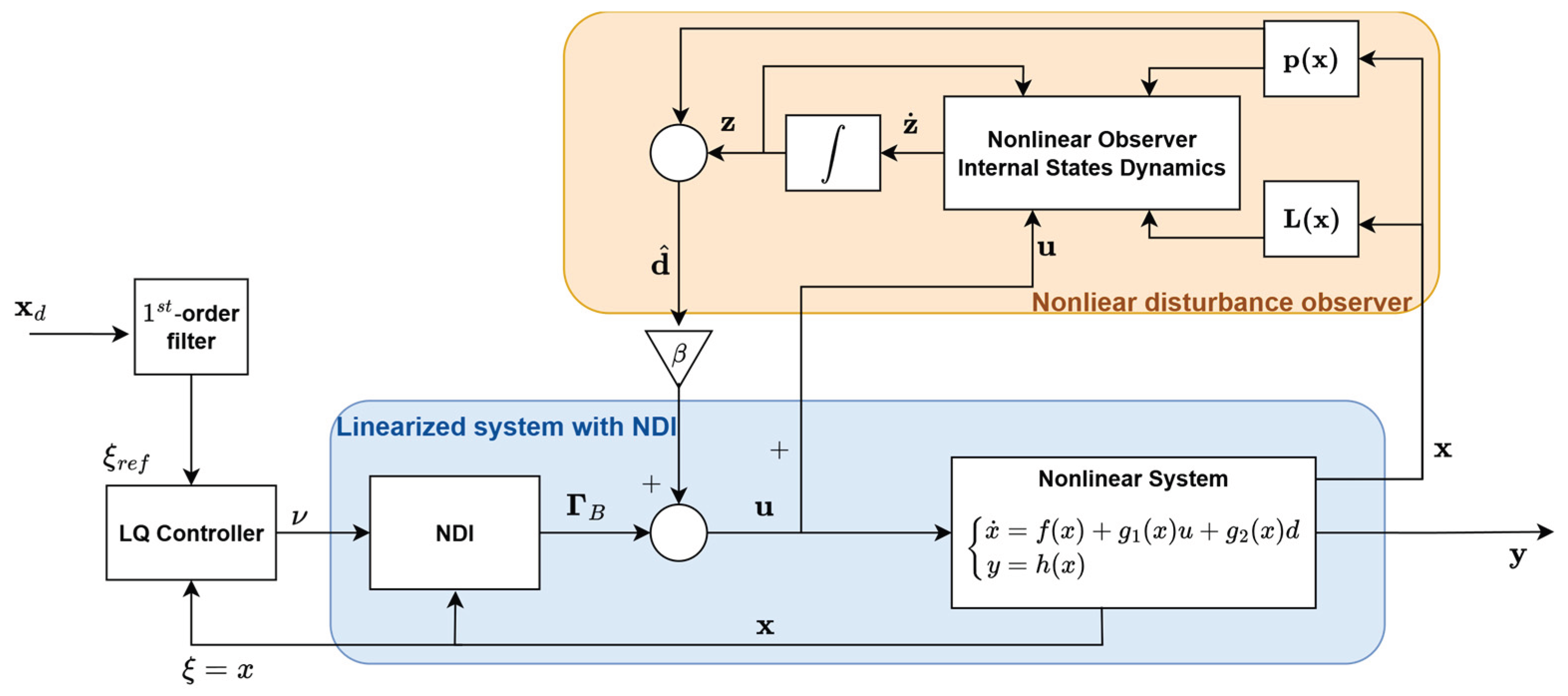
Figure 2.
Illustration of the gravity disturbance acting on the attitude control testbed. The misalignment of the center of gravity and the center of air bearing causes a disturbance torque.
Figure 2.
Illustration of the gravity disturbance acting on the attitude control testbed. The misalignment of the center of gravity and the center of air bearing causes a disturbance torque.
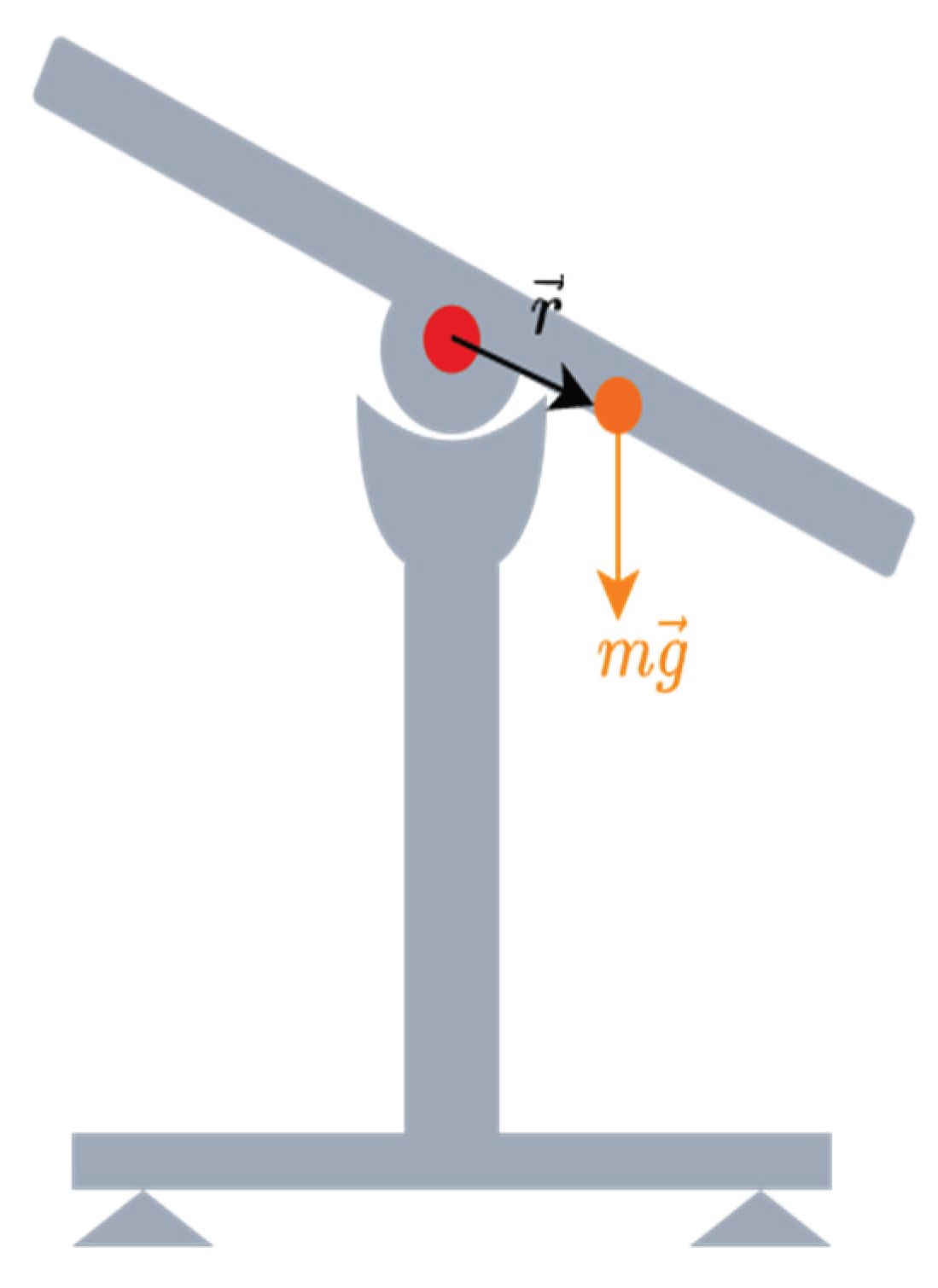
Figure 3.
Comparison of quaternion simulation results between the proposed NDI and Bang’s method [8]. The proposed method (red) outperforms Bang’s method (blue) during the transient phase by providing a smooth convergence without oscillatory overshoots.
Figure 3.
Comparison of quaternion simulation results between the proposed NDI and Bang’s method [8]. The proposed method (red) outperforms Bang’s method (blue) during the transient phase by providing a smooth convergence without oscillatory overshoots.
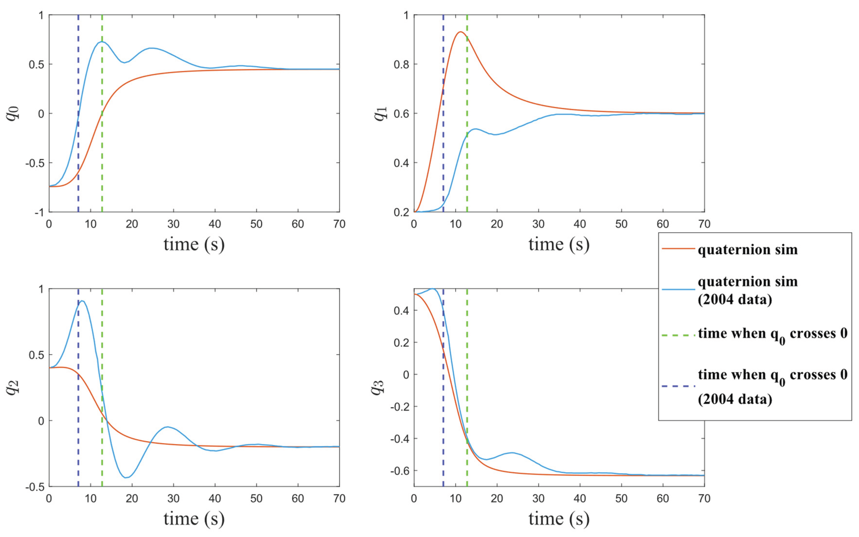
Figure 4.
Comparison of control input derivatives between the proposed NDI and Bang’s method [8]. While Bang’s method (blue) suffers from severe numerical instability – evidenced by the massive spike when crosses zero – the proposed NDI method (red) successfully avoids this singularity, maintaining smooth and bounded control input derivatives.
Figure 4.
Comparison of control input derivatives between the proposed NDI and Bang’s method [8]. While Bang’s method (blue) suffers from severe numerical instability – evidenced by the massive spike when crosses zero – the proposed NDI method (red) successfully avoids this singularity, maintaining smooth and bounded control input derivatives.
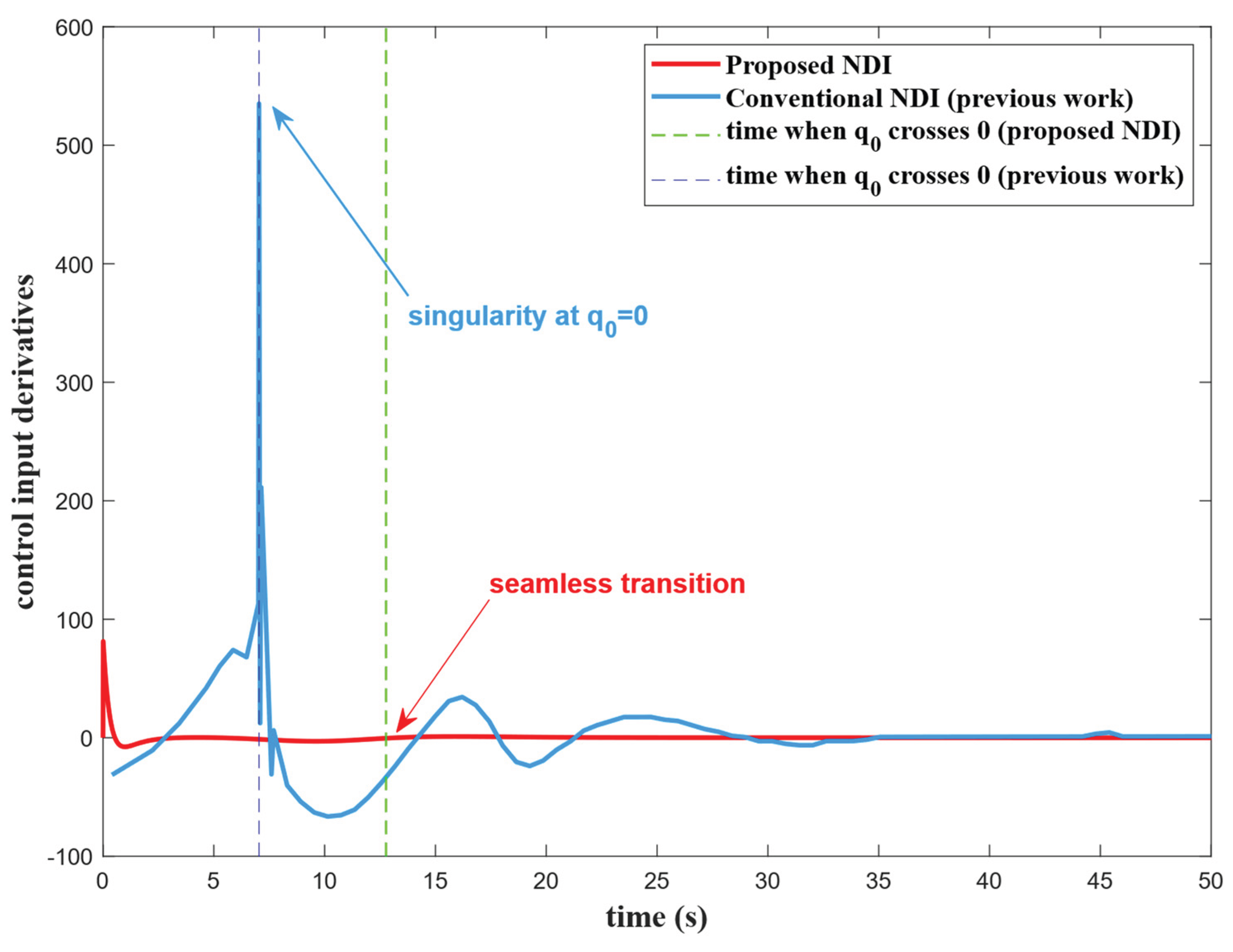
Figure 5.
Quaternion simulation results utilizing a reduced time constant (). The proposed exact input-state linearization method (red) allows for significantly faster attitude convergence while completely eliminating the oscillatory overshoots present in conventional formulations (blue).
Figure 5.
Quaternion simulation results utilizing a reduced time constant (). The proposed exact input-state linearization method (red) allows for significantly faster attitude convergence while completely eliminating the oscillatory overshoots present in conventional formulations (blue).
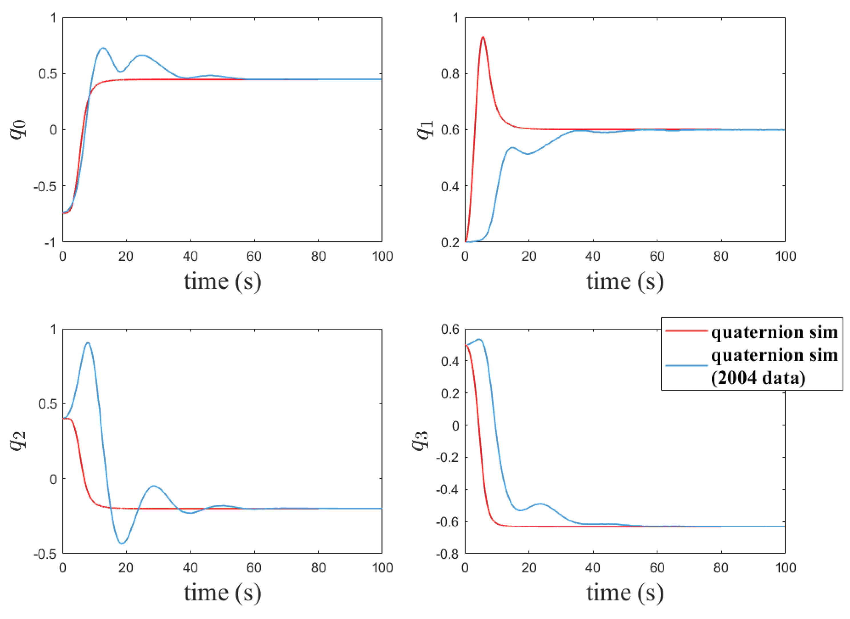
Figure 6.
Comparison of control input derivatives under accelerated tracking (). Despite the aggressive tracking requirements of the smaller time constant, the proposed NDI framework (red) seamlessly navigates the crossing without singularity spikes, maintaining strictly bounded control efforts and successfully preventing actuator saturation.
Figure 6.
Comparison of control input derivatives under accelerated tracking (). Despite the aggressive tracking requirements of the smaller time constant, the proposed NDI framework (red) seamlessly navigates the crossing without singularity spikes, maintaining strictly bounded control efforts and successfully preventing actuator saturation.
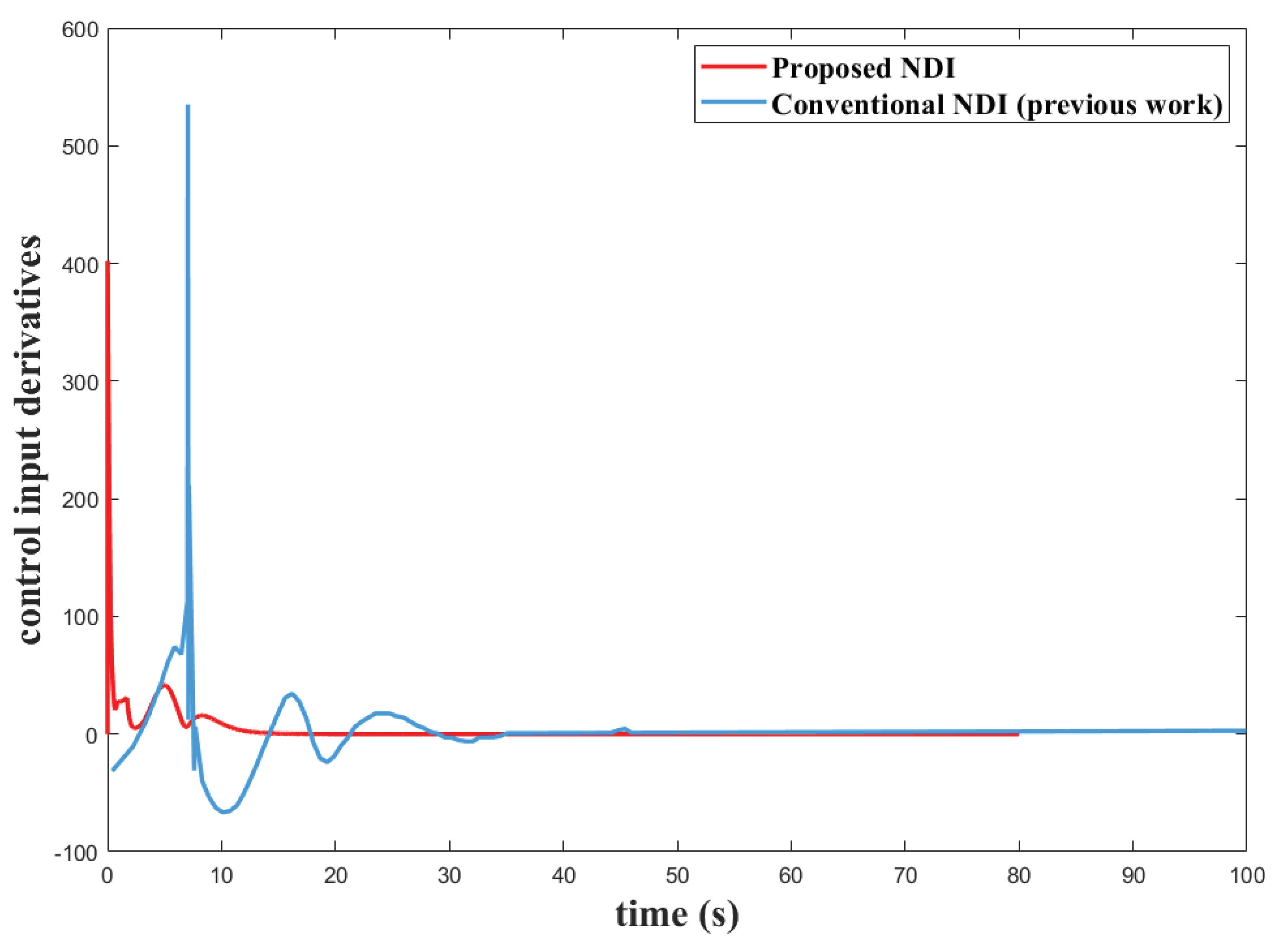
Figure 7.
Quaternion simulation results under different mismatched moments of inertia. This simulation evaluates the system’s performance under three distinct moment of inertia matrices (, , and ), while the NDI is derived based on the nominal matrix . As observed, although varying the inertia matrices yields different transient trajectories, the combined NDI and LQ controller successfully regulates the quaternions to the desired reference states. These results effectively validate the controller’s robustness against inertial model mismatches.
Figure 7.
Quaternion simulation results under different mismatched moments of inertia. This simulation evaluates the system’s performance under three distinct moment of inertia matrices (, , and ), while the NDI is derived based on the nominal matrix . As observed, although varying the inertia matrices yields different transient trajectories, the combined NDI and LQ controller successfully regulates the quaternions to the desired reference states. These results effectively validate the controller’s robustness against inertial model mismatches.
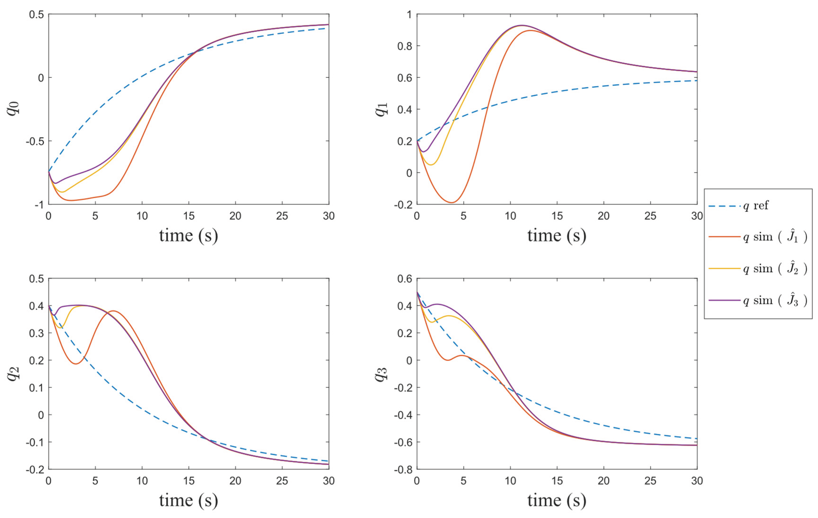
Figure 8.
Disturbance estimation error with different observer gains. While a higher gain () yields a faster initial response, it introduces undesirable transient oscillations. Therefore, demonstrates the optimal balance, ensuring rapid convergence while maintaining transient smoothness.
Figure 8.
Disturbance estimation error with different observer gains. While a higher gain () yields a faster initial response, it introduces undesirable transient oscillations. Therefore, demonstrates the optimal balance, ensuring rapid convergence while maintaining transient smoothness.
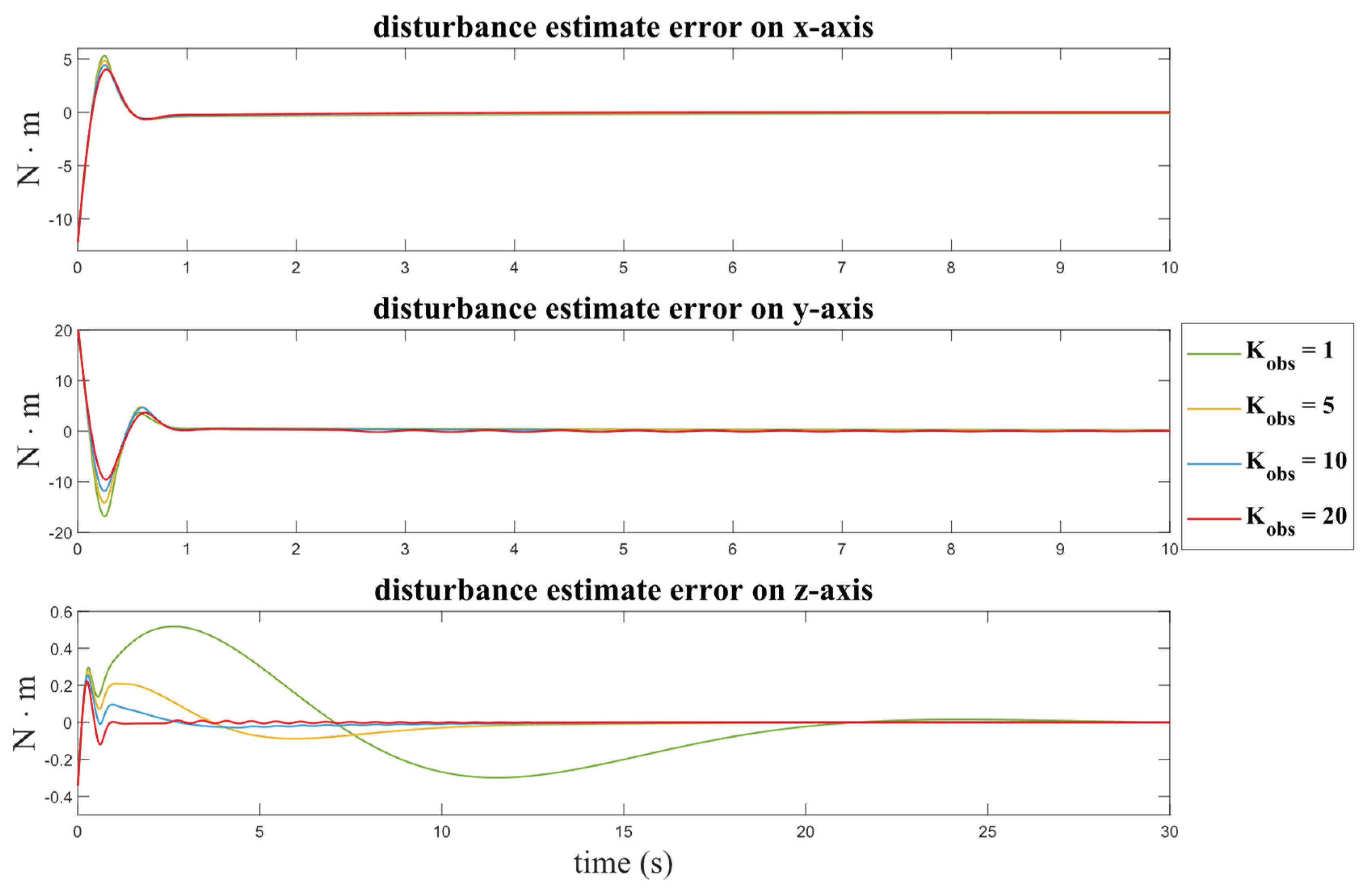
Figure 9.
Quaternion simulation results with different observer gains. The trajectories indicate that although increasing improves the speed of convergence to the reference, it induces undesirable transient oscillations, which is particularly for .
Figure 9.
Quaternion simulation results with different observer gains. The trajectories indicate that although increasing improves the speed of convergence to the reference, it induces undesirable transient oscillations, which is particularly for .
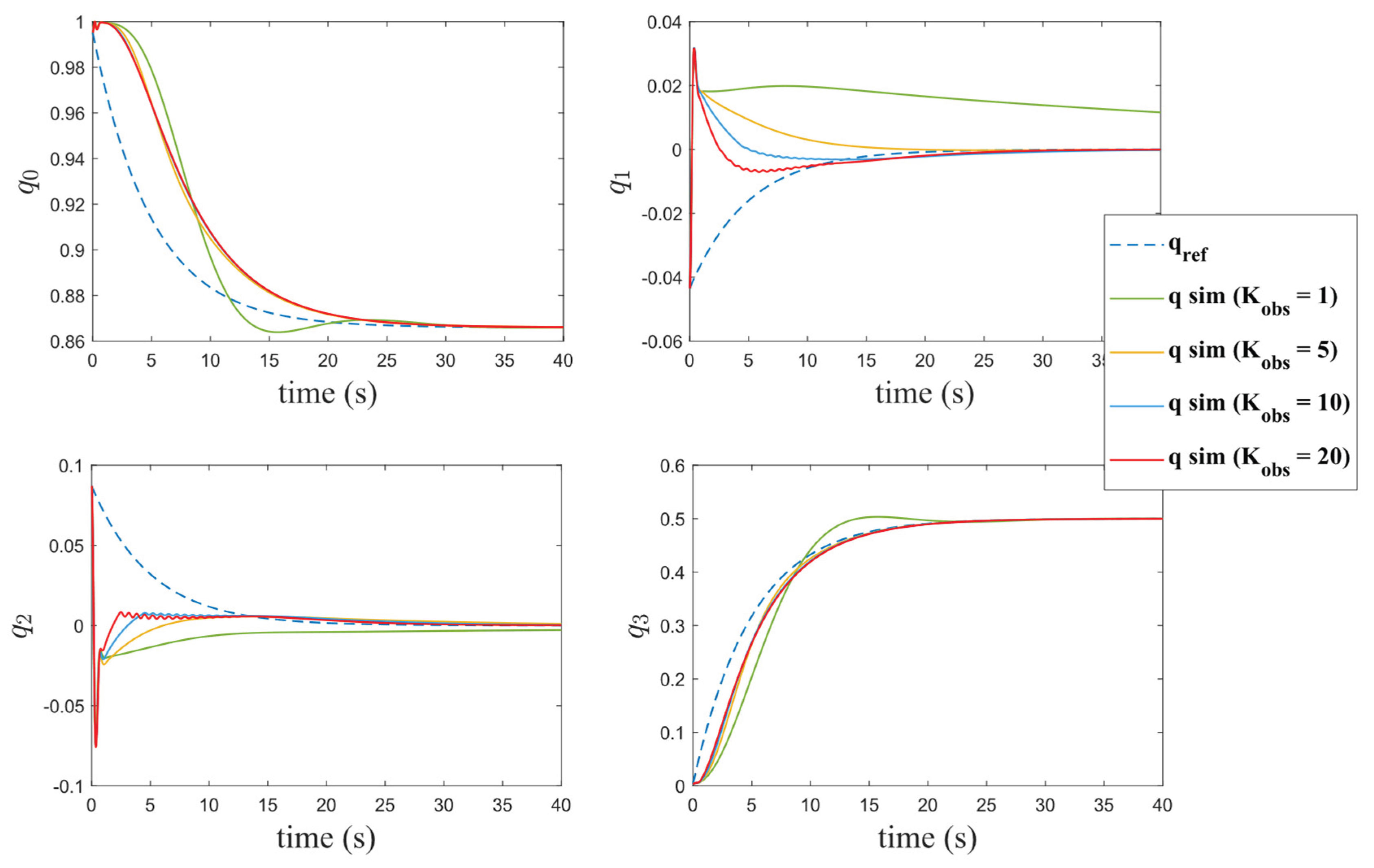
Figure 10.
Euler angle representation of the simulation results fromFigure 9. The plots demonstrate that both extreme gains yield suboptimal performance: fails to eliminate the steady-state error, whereas induces noticeable transient oscillations in the control response.
Figure 10.
Euler angle representation of the simulation results fromFigure 9. The plots demonstrate that both extreme gains yield suboptimal performance: fails to eliminate the steady-state error, whereas induces noticeable transient oscillations in the control response.
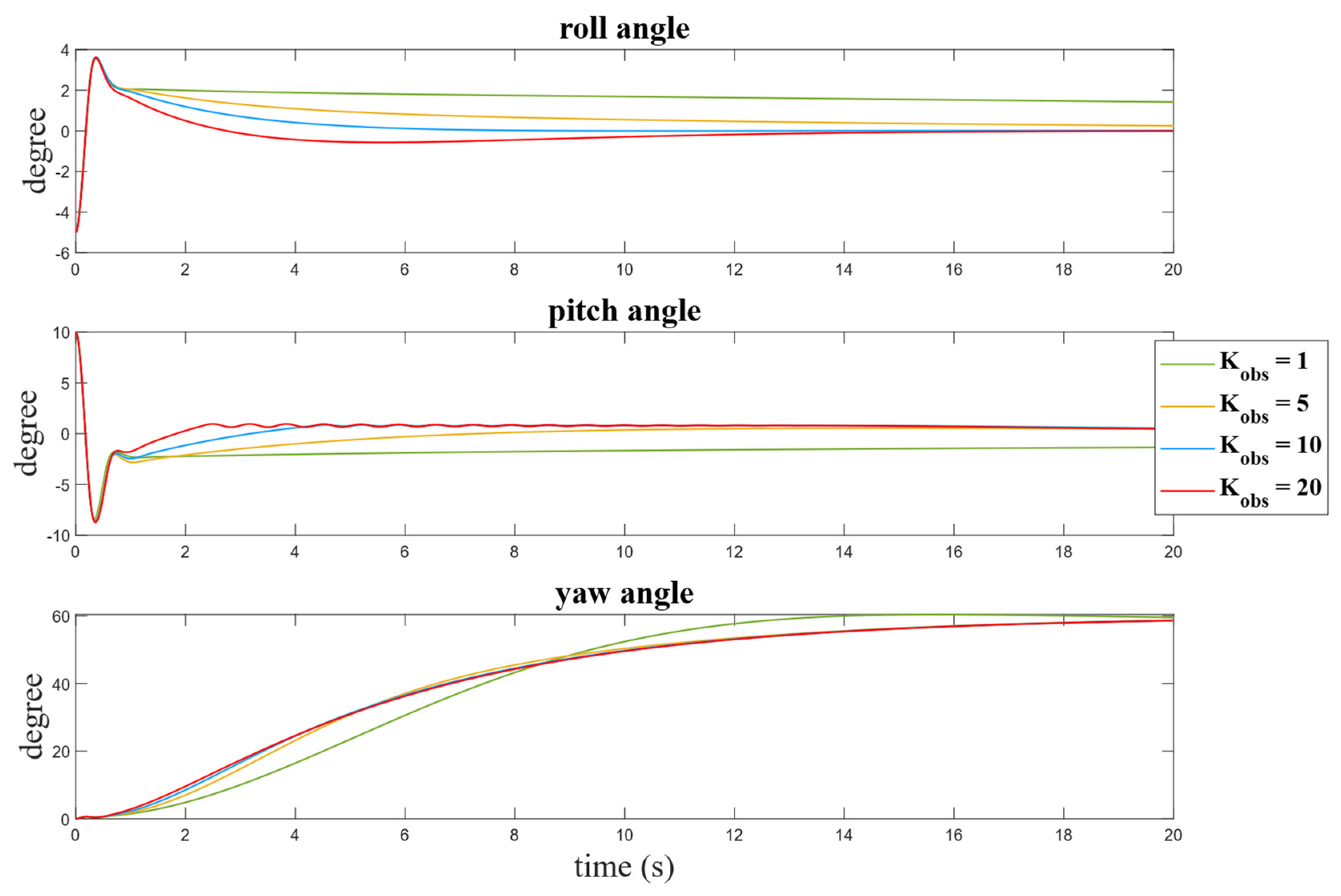
Figure 11.
Euler angle response of the attitude testbed using the proposed NDI and DOBC framework. The results demonstrate that the controller successfully achieves the target attitude, effectively compensating for both model mismatches and external disturbances.
Figure 11.
Euler angle response of the attitude testbed using the proposed NDI and DOBC framework. The results demonstrate that the controller successfully achieves the target attitude, effectively compensating for both model mismatches and external disturbances.
Disclaimer/Publisher’s Note: The statements, opinions and data contained in all publications are solely those of the individual author(s) and contributor(s) and not of MDPI and/or the editor(s). MDPI and/or the editor(s) disclaim responsibility for any injury to people or property resulting from any ideas, methods, instructions or products referred to in the content. |
© 2026 by the authors. Licensee MDPI, Basel, Switzerland. This article is an open access article distributed under the terms and conditions of the Creative Commons Attribution (CC BY) license (http://creativecommons.org/licenses/by/4.0/).
Copyright: This open access article is published under a Creative Commons CC BY 4.0 license, which permit the free download, distribution, and reuse, provided that the author and preprint are cited in any reuse.


