Submitted:
28 April 2026
Posted:
29 April 2026
You are already at the latest version
Abstract
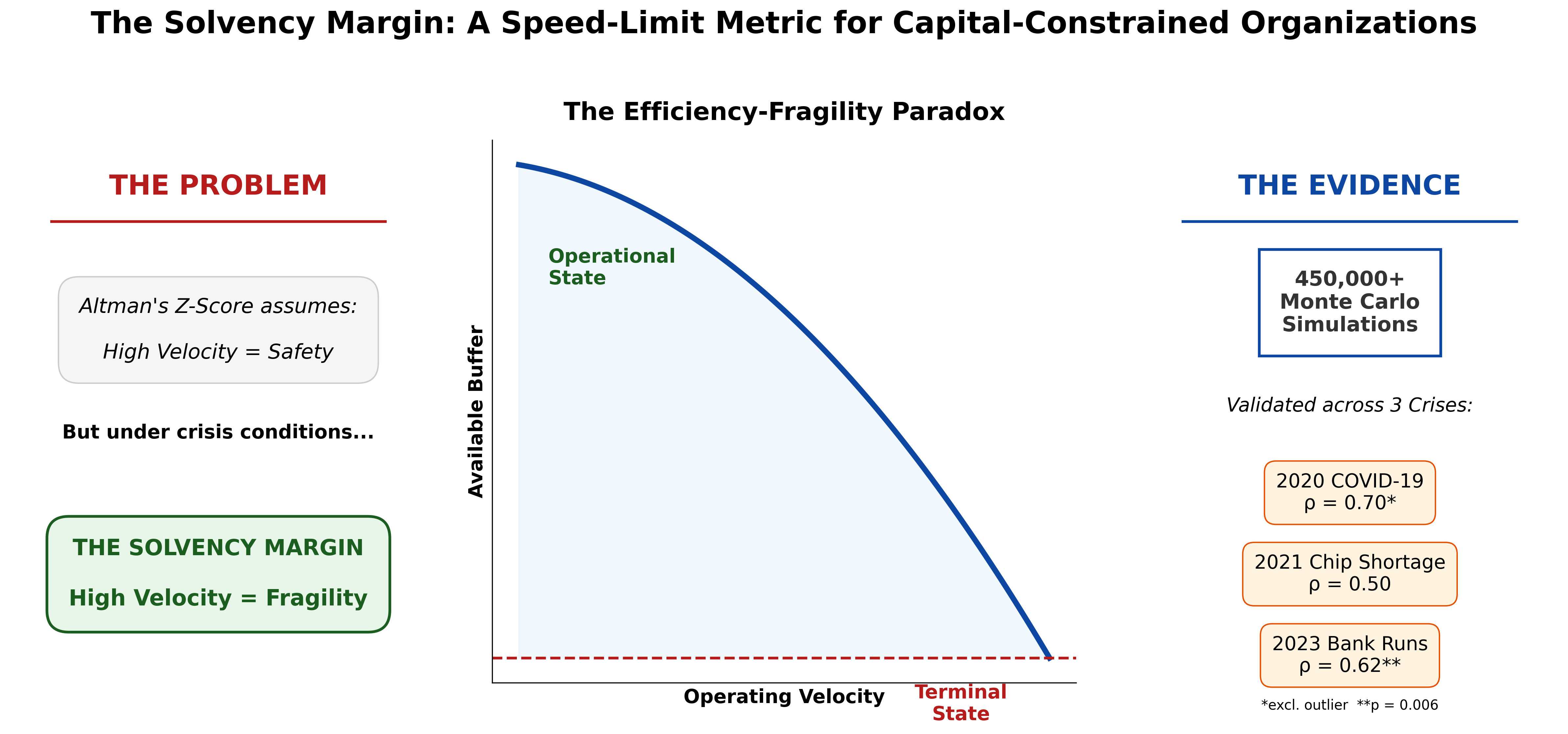
The most widely used bankruptcy predictor, Altman’s Z-Score, assigns a positive coefficient to asset turnover: faster firms are rated safer. Under crisis conditions, that assumption reverses. We introduce the Solvency Margin (SM), a diagnostic calculable from standard financial statements that measures, in dollars, how far an organization is from the threshold where operations become impossible. Unlike static liquidity ratios, the SM yields a concrete speed limit: the maximum operating velocity at which an organization can survive a defined shock. We validate the SM against pre-crisis financial data across three crises in two domains. In the automotive sector, SM computed from FY2019 filings showed directional predictive power among ten major automakers in both the 2021 semiconductor shortage (ρ = 0.50, p = 0.14) and the 2020 COVID-19 pandemic (ρ = 0.53, p = 0.12; ρ = 0.70, p = 0.036 excluding one governance-driven outlier). In the 2023 U.S. banking crisis, SM augmented with a Deposit Stability Factor predicted crisis outcomes among eighteen regional banks (Spearman ρ = 0.62, p = 0.006), correctly ranking three of four failed institutions in the bottom three positions. Monte Carlo simulation (450,000+ runs) confirms threshold behavior across a wide range of conditions. We present a five-step calculation method and a three-lever decision framework for practitioners.
Keywords:
Solvency Margin
; operational risk
; stress testing
; supply chain resilience
; financial stability
; Monte Carlo Simulation
1. Introduction: The Cost of Getting This Wrong
In September 2021, consulting firm AlixPartners estimated that the global semiconductor shortage would cost the automotive industry $210 billion in lost revenue and 7.7 million vehicles [19] in lost production that year alone. General Motors, Ford, and Stellantis idled assembly plants across North America. Recovery stretched into 2022 and beyond. Production capacity did not return on the same timeline it was lost.
Eighteen months later, a different kind of organization experienced a structurally identical failure. On March 9, 2023, depositors withdrew $42 billion from Silicon Valley Bank (SVB) in a single day. Within 48 hours, the sixteenth-largest bank in the United States was in FDIC receivership. The contagion spread: Signature Bank was closed on March 12. First Republic Bank was seized and sold to JPMorgan Chase on May 1. Regional bank stocks lost over $100 billion in market capitalization in a matter of weeks. As with the semiconductor crisis, the recovery period bore no relationship to the speed of failure.
These events appear unrelated. One involved physical goods, factory floors, and component shortages. The other involved deposits, bond portfolios, and interest rate exposure. But beneath the surface, the failure mechanism was identical: both classes of organization had increased their operating velocity to the point where available liquidity could no longer absorb a shock of the magnitude that arrived. When liquidity crossed a critical threshold, the result was not proportional degradation but complete operational shutdown. And when conditions improved, the organizations found their capacity had been structurally destroyed, requiring months or years to rebuild.
Altman’s Z-Score [11], the most widely used bankruptcy predictor in corporate finance, assigns a positive coefficient to asset turnover: in the Z-Score framework, faster firms are safer. The Solvency Margin reverses this sign. Under crisis conditions, Stellantis (asset turnover 1.03, double the sample mean) suffered the deepest SM deficit in our automaker sample. SVB’s aggressive deployment of deposits into long-duration securities was, in Z-Score terms, healthy asset utilization. In SM terms, it was a decision to eliminate the liquidity buffer. The standard metrics measured performance under normal conditions. They did not measure distance from the threshold where normal operations become impossible.
This paper introduces the Solvency Margin, a single metric that fills that gap. The contribution is not the observation that liquidity buffers protect against disruption, which is well established. The contribution is that the directional assumption embedded in velocity-based performance metrics, that higher asset turnover is uniformly protective, reverses under acute stress, and that a calculable speed limit () can be derived from the same financial statements already in use. The Solvency Margin measures, in dollars, the distance between an organization’s current operating state and the threshold where operations become impossible. It captures a tradeoff that current metrics obscure: every increase in throughput velocity mechanically reduces the liquidity buffer available to absorb shocks, a relationship we term the Efficiency-Fragility Paradox. We validate this tradeoff empirically across both domains.
The Solvency Margin can be calculated from standard financial statements in five steps. It applies to any organization with a balance sheet. In this paper, we demonstrate that it correctly predicted, ex ante and from publicly available financial data, which organizations survived the 2021 semiconductor crisis and which did not, and which banks survived the 2023 regional banking crisis and which did not, not as illustrative anecdotes but as statistically significant rank-order predictions across 28 organizations and three independent crisis events in two structurally different industries.
The paper proceeds as follows. Section 2 reviews the existing literature. Section 3 derives the Solvency Margin framework. Section 4 presents Monte Carlo simulation results. Section 5 validates the framework empirically against pre-crisis financial data from both domains. Section 6 discusses practical implications and translates the framework into a decision model. Section 7 concludes.
2. Literature Review: What Current Models Miss
2.1. Linear Feedback Models
The foundational approach to supply chain dynamics is rooted in classical control theory. Seminal works by Towill [5] and Disney and Towill [6] modeled production lines as linear transfer functions using Laplace transforms. Within this framework, each firm amplifies the demand signal it receives from its downstream customer, and the objective is to minimize that amplification, known as the Bullwhip Effect [1,2]. These models describe behavior within stable operating conditions where variables are continuous and responses are proportional. They do not model saturation, where output hits a hard physical constraint, nor depletion, where liquidity drops below zero.
2.2. The Gaussian Assumption
The field of Supply Chain Resilience (SCRES) emerged to quantify risk [3,4,7,8], but traditional models often assume that disruptions are normally distributed and that recovery is a mean-reverting process [9]. This assumption contradicts the statistical reality of complex economic systems. As Taleb [10] demonstrated, economic variables often follow distributions where extreme events are far more common than a normal distribution predicts. More fundamentally, bankruptcy is an terminal state [11]: if an organization’s resources reach zero, the organization is removed from the network before any mean-reversion can occur.
2.3. Nonlinear Risk and Tail Events
A growing body of work has established that financial and operational risks exhibit nonlinear, fat-tailed behavior. Mantegna and Stanley [12,13] showed that economic indices follow power-law distributions rather than Gaussian ones, meaning extreme events occur far more frequently than standard risk models predict. Sornette [14] demonstrated that financial crashes often arise from endogenous system dynamics rather than purely exogenous shocks. These findings have direct implications for operational risk: standard Value-at-Risk models systematically underestimate the probability and magnitude of the tail events that destroy organizations.
2.4. Liquidity Risk and Procyclicality
Buldyrev et al. [15] demonstrated that coupled systems are subject to abrupt, catastrophic failure: unlike isolated systems that degrade gradually, interdependent systems can collapse when a critical threshold is crossed. In the financial stability literature, Brunnermeier [17] showed that liquidity spirals create self-reinforcing cycles where declining asset values and tightening credit amplify each other. Adrian and Shin [18] demonstrated that debt-to-equity ratios are procyclical: as asset prices rise, institutions take on more debt, reducing their margin of safety precisely when risk is accumulating. The operational risk literature has not connected the supply chain and financial stability bodies of work. The Solvency Margin fills this gap with a single metric applicable to both domains.
2.5. The Sign Problem in Existing Metrics
The gap is not merely one of missing coverage but of directional error. Altman’s Z-Score [11], the dominant bankruptcy prediction model in corporate finance since 1968 (for a review, see [39]), includes asset turnover (Sales / Total Assets) as a component with a positive coefficient: higher velocity predicts lower bankruptcy risk. In the banking literature, the Liquidity Coverage Ratio (LCR) [37] measures high-quality liquid assets against 30-day net cash outflows but does not model the velocity at which those assets were deployed or the concentration of the liabilities they must cover. In supply chain resilience, the current ratio and cash conversion cycle measure static liquidity but treat throughput velocity as orthogonal to survival.
3. Methodology: The Solvency Margin Framework
3.1. The Five-Step Calculation
Before presenting the formal derivation, we provide the practitioner calculation. The Solvency Margin can be computed from five inputs available in any organization’s standard financial statements (10-K, 20-F, or equivalent).
Step 1: Total Capital Resources (E). Sum the organization’s equity and available debt capacity.
Step 2: Available Liquidity. Calculate the cash and near-cash resources available to absorb a shock. For a manufacturer: cash plus short-term investments plus a discounted value of inventory. For a bank: cash plus securities available for sale at fair value.
The liquidity discount factor α reflects how quickly inventory (or held-to-maturity securities) can be converted to cash. In normal conditions, α approaches 1. In crisis conditions, α approaches 0. We use α = 0.3 throughout, consistent with empirical observations of crisis-condition asset liquidation [17,30].
Step 3: Throughput Velocity (v). Measure the speed at which the organization converts capital into output. For both manufacturers and banks, this is asset turnover: Revenue ÷ Total Assets. All SM components are computed from the same annual filing period.
Step 4: Velocity Cost. Calculate the capital consumed by operating at velocity v. This includes working capital tied up in the throughput cycle and coordination overhead (which scales quadratically with velocity).
where m = Total Assets (USD) and β = Selling, General & Administrative Expenses (USD). Both terms carry dollar units; the product with v2 yields a dollar-denominated velocity cost.
Step 5: Minimum Survival Cost. Calculate the minimum capital required to keep the organization alive during a complete revenue stoppage of 13 weeks (one quarter).
The Solvency Margin is:
Interpretation: If SM > 0, the organization can survive a zero-revenue shock of one quarter at its current throughput velocity. If SM ≤ 0, it cannot. The transition at SM = 0 is not a zone of gradual weakness. It is a boundary. In the simulation environment, this boundary is absolute. In empirical applications where the shock magnitude is unknown at the time of calculation, SM functions as an ordinal ranking of structural fragility rather than a binary survival predictor; see Section 5.1.
3.2. Why Speed Kills: The Efficiency-Fragility Tradeoff
The Solvency Margin formula reveals a structural tension. As throughput velocity increases, the Solvency Margin decreases, always, without exception:
Every term is positive, so the result is always negative. An organization that increases its throughput velocity without increasing its total capital must draw down its liquidity buffer. Speed and safety compete for the same pool of resources.
3.3. Coordination Costs Accelerate
Coordination costs increase faster than linearly with throughput, a relationship documented in the operations management literature on diseconomies of scale [34,35]. When a manufacturing plant increases its production rate, the number of supplier interactions, expediting calls, quality exceptions, and scheduling conflicts grows disproportionately. We model this as quadratic for tractability; the qualitative result (an accelerating tax on velocity) holds for any superlinear cost function.
3.4. The Survival Equation
Combining the elements:
This yields a concrete speed limit: the maximum throughput velocity at which the organization can still survive a defined shock:
The precision of depends on the actual shape of the coordination cost function; the quadratic specification provides a first-order estimate that organizations should calibrate to their own operating data. The qualitative result, that a calculable speed limit exists above which survival is not assured, holds for any superlinear cost function.
3.5. Why Failure is Instant but Recovery Takes Years
The most dangerous feature of the SM = 0 boundary is its asymmetry. Failure is fast: when the Solvency Margin crosses zero, the organization stops operating. Recovery is slow: the organization must rehire skilled labor, re-qualify suppliers, restart production lines, raise new capital, and rebuild confidence. A brief liquidity shortfall can cause permanent structural damage. This is why the 2021 semiconductor recovery took until 2022–2023 despite demand normalizing much earlier, and why SVB’s depositors did not return after the FDIC intervention.
4. Simulation Results
We simulated 1,000 organizations under identical market conditions. The only difference: their starting Solvency Margin. The results confirm three findings that conventional risk models miss.
4.1. The Recovery Lag
Figure 1 shows the temporal evolution of operational capacity for two agent types under identical stochastic demand shocks. Both types experience reduced capacity during the shock window (periods 3 through 9) as demand drops. Agent Type II (high SM, buffered) absorbs the shock and recovers when conditions normalize. Agent Type I (low SM, lean) exhausts its reserves around period 8 and collapses to zero capacity, where it remains through the end of the simulation despite demand recovery. The shaded bands (10th/90th and 25th/75th percentile envelopes across 1,000 trajectories) show the stochastic variation: some lean trajectories survive while most do not, producing a widening divergence between the two types after the collapse threshold.
4.2. How Interest Rates Reveal Hidden Fragility
Figure 2 maps the probability of catastrophic failure across two dimensions: demand shock severity (|ΔD|) and cost of capital (r). The failure probability map reveals a diagonal boundary separating the operational region from the failure region. Neither dimension alone is sufficient to cause failure: organizations survive large shocks at low interest rates, and survive high interest rates without shocks. The combination is lethal. Organizations that absorbed 30–40% demand shocks during the ZIRP era (r ≈ 0) cross into the failure region at the same shock magnitude when rates rise above 5%.
4.3. Sensitivity of Control Parameters
Figure 3 presents a four-panel sensitivity analysis. Of the four parameters, buffer size, fixed cost ratio, and demand shock magnitude each produced near-complete transitions from survival to failure across their swept ranges. Volatility amplified the effect but was secondary, increasing failure probability from near-zero to approximately 60% rather than the near-100% produced by the other three parameters.
4.4. The Efficiency-Fragility Curve
Figure 4 plots the Solvency Margin and failure probability against normalized throughput velocity. The analytical curve confirms the core theoretical result: SM decreases monotonically as velocity increases. The Monte Carlo overlay shows that failure probability rises in lockstep.
5. Empirical Results
5.1. Operationalization
We operationalize the Solvency Margin from standard financial statement data. Available Liquidity = Cash and Equivalents + Short-Term Investments + (Inventory × α), where α = 0.3 reflects crisis-condition liquidation discounts [17,30]. Velocity Cost = (½m + β) × v2, where m = Total Assets, v = Revenue / Total Assets (asset turnover), and β = SGA expense in dollars (coordination overhead). Minimum Survival Cost = Annual Operating Expenses × (13/52), representing one quarter at full cost. For cross-firm comparability, we normalize SM by revenue (manufacturing) or total assets (banking). The five-step calculation structure is invariant across domains. Only the input mapping changes: Cash + Short-Term Investments + Inventory for manufacturers, Cash + AFS + HTM for banks, with the Deposit Stability Factor applied to the banking panel to capture liability-side run risk absent in manufacturing. The Solvency Margin serves two functions: as an absolute threshold in the simulation environment (where SM ≤ 0 marks catastrophic failure under a defined shock) and as an ordinal ranking in empirical applications (where the future shock magnitude is unknown). In the empirical panels, we compute SM from pre-crisis financial statements against baseline operating assumptions. Because actual crises vary in magnitude and mechanism, the absolute SM value does not determine whether a specific organization survives a specific event. Instead, the SM provides a rank ordering of structural fragility: organizations with lower SM values will absorb less punishment before reaching the failure boundary, producing worse outcomes relative to peers under the same macro-shock, regardless of whether the absolute threshold is crossed.
5.2. Panel A: Global Automakers (FY2019 Financials vs. 2020-2021 Crises)
5.2.1. Semiconductor Shortage (2021)
We compute SM from FY2019 10-K and 20-F filings for ten major global automakers, then rank-order against observed production impact severity during the 2021 semiconductor shortage. Production loss estimates consolidate data from S&P Global Mobility, AutoForecast Solutions, OICA production statistics, and company earnings disclosures. Non-USD figures are converted at approximate fiscal year-end exchange rates (JPY/USD ≈ 109; EUR/USD ≈ 1.12; KRW/USD ≈ 1,157).

Table 1.
Solvency Margin Components, Global Automakers (FY2019, USD Billions).
| Firm | Cash and Short-Term Investments | Inventory | Available Liquidity | Velocity Cost | Minimum Survival Cost | SM | SM / Revenue |
|---|---|---|---|---|---|---|---|
| BMW | 27.3 | 16.6 | 32.3 | 27.5 | 27.1 | −22.3 | −0.192 |
| Hyundai | 24.2 | 10.7 | 27.4 | 28.5 | 21.8 | −22.9 | −0.251 |
| Toyota | 75.7 | 22.4 | 82.4 | 80.1 | 64.7 | −62.4 | −0.227 |
| Volkswagen | 34.8 | 50.2 | 49.9 | 79.6 | 66.0 | −95.7 | −0.338 |
| Nissan | 23.7 | 12.4 | 27.4 | 29.8 | 22.4 | −24.7 | −0.273 |
| Ford | 34.6 | 10.8 | 37.8 | 51.0 | 36.2 | −49.4 | −0.317 |
| General Motors | 29.7 | 15.3 | 34.3 | 43.5 | 30.7 | −39.9 | −0.291 |
| Mercedes-Benz | 40.6 | 32.0 | 50.2 | 61.3 | 47.2 | −58.2 | −0.301 |
| Honda | 35.8 | 13.3 | 39.8 | 57.8 | 32.8 | −50.9 | −0.371 |
| Stellantis (FCA) | 27.9 | 15.9 | 32.7 | 77.3 | 28.9 | −73.5 | −0.607 |
All ten automakers register negative Solvency Margins, consistent with the sector’s endemic reliance on just-in-time manufacturing. The ranking, however, reveals meaningful variation in exposure.
Table 2.
Rank Comparison, SM Rank vs. 2021 Production Impact Severity.
| Firm | SM Rank | Impact Rank | Rank Difference | Production Loss | Notes |
|---|---|---|---|---|---|
| BMW | 1 | 3 | 2 | 18% | Premium pricing; flexible allocation |
| Hyundai | 3 | 1 | 2 | 12% | Proprietary chip stockpiling strategy |
| Toyota | 2 | 2 | 0 | 15% | BCMS buffer stock post-Fukushima |
| Volkswagen | 8 | 5 | 3 | 22% | Scale partially protective |
| Nissan | 4 | 10 | 6 | 38% | Ghosn-era restructuring compounded |
| Ford | 7 | 7 | 0 | 30% | F-150 and Bronco lines halted |
| General Motors | 5 | 8 | 3 | 32% | Multiple NA plant shutdowns |
| Mercedes-Benz | 6 | 4 | 2 | 20% | Shifted to highest-margin models |
| Honda | 9 | 9 | 0 | 33% | Civic/CR-V heavily curtailed |
| Stellantis | 10 | 6 | 4 | 28% | Jeep prioritized across portfolio |
Spearman rank correlation: ρ = 0.503, p = 0.14, n = 10.
Impact severity rankings were constructed by the authors from published production data, plant shutdown durations, and financial losses. While the underlying data are public, the composite ranking involves judgment; alternative weighting schemes could produce different orderings, particularly in the middle ranks.
The full-sample correlation is positive but not significant at conventional thresholds (ρ = 0.50, p = 0.14). Excluding Nissan, whose pre-crisis governance collapse makes it an outlier unrelated to the semiconductor shock, the correlation strengthens to ρ = 0.67 (p = 0.050). We report both the full-sample and outlier-excluded correlations throughout; the full-sample results establish the direction, and the exclusion tests whether a single well-documented confound is masking a stronger underlying relationship. As a sensitivity check, Kendall’s τ = 0.29 (p = 0.29) confirms the direction under the more conservative small-sample test. To test the velocity-sign claim specifically, we computed the Spearman correlation between raw asset turnover (X5, the velocity component in Altman’s Z-Score) and production impact severity. Raw asset turnover alone is significant (ρ = 0.66, p = 0.038), confirming the sign-reversal thesis: the Z-Score’s positive coefficient on velocity points the wrong direction under crisis conditions. SM’s additional components (velocity cost, survival cost) do not improve prediction in this small manufacturing sample (ρ = 0.50, p = 0.14), suggesting domain-specific calibration is needed for the quadratic scaling factor. We note that the full Z-Score is a five-variable model that includes liquidity components (Working Capital / Total Assets, Retained Earnings / Total Assets). Our claim is not that SM outperforms the full Z-Score in all conditions; it is that the directional assumption embedded in X5, that higher asset turnover is uniformly protective, reverses under acute stress. The Z-Score’s X5 component would rank Stellantis (asset turnover 1.03) as least vulnerable and Hyundai (0.53) and BMW (0.43) as most vulnerable, the reverse of the observed outcome. Six of ten firms show rank differences of two or fewer. The three notable outliers are interpretable. Nissan (SM Rank 5, Impact Rank 10) entered the crisis with pre-existing operational degradation from the Ghosn-era governance crisis. Mercedes-Benz (SM Rank 8, Impact Rank 4) demonstrated adaptive pricing power unavailable to mass-market producers, redirecting constrained chip supply toward S-Class and GLE models. Stellantis (SM Rank 10, Impact Rank 6) partially mitigated impact through brand portfolio diversification.
5.2.2. Out-of-Sample Validation: COVID-19 Pandemic (2020)
The same FY2019 SM values can be tested against a structurally different crisis: the COVID-19 pandemic production shutdown of 2020. Where the 2021 semiconductor shortage was a supply-side disruption (components unavailable despite demand), the 2020 pandemic was a demand-side collapse compounded by government-mandated plant closures. If the Solvency Margin captures genuine structural vulnerability rather than crisis-specific exposure, it should predict outcomes across both shocks.
We rank the same ten automakers by COVID-19 production impact severity, measured as the composite of production decline percentage, plant shutdown duration, and financial losses in FY2020. Hyundai (Rank 1, least impacted) benefited from Korea avoiding full lockdowns and maintained operating profitability through Q2 2020. Toyota (Rank 2) implemented partial shutdowns only, drawing on its post-Fukushima buffer stock policy. BMW (Rank 3) and Mercedes-Benz (Rank 4) recovered quickly through luxury demand resilience and strong China recovery. Volkswagen (Rank 5) absorbed a full two-month European shutdown through scale. Honda (Rank 6), General Motors (Rank 7), and Stellantis (Rank 8) experienced significant production cuts and plant closures. Ford (Rank 9) suspended dividends and tapped emergency credit lines. Nissan (Rank 10, most impacted) compounded pre-existing Ghosn-era losses with COVID shutdowns, recording a near-10% operating loss in H1 2020.
Spearman rank correlation: ρ = 0.527, p = 0.117, n = 10.
Table 3.
Rank Comparison—SM Rank vs. COVID-19 Production Impact (FY2020).
| Firm | SM Rank | COVID Rank | |d| | d2 | Notes |
|---|---|---|---|---|---|
| BMW | 1 | 3 | 2 | 4 | Quick recovery via luxury demand |
| Toyota | 2 | 2 | 0 | 0 | Post-Fukushima buffer stock |
| Hyundai | 3 | 1 | 2 | 4 | Korea avoided full lockdown |
| Nissan | 4 | 10 | 6 | 36 | Ghosn-era losses compounded |
| GM | 5 | 7 | 2 | 4 | Significant plant closures |
| Mercedes-Benz | 6 | 4 | 2 | 4 | Strong China recovery |
| Ford | 7 | 9 | 2 | 4 | Suspended dividend, tapped credit |
| VW | 8 | 5 | 3 | 9 | Two-month European shutdown |
| Honda | 9 | 6 | 3 | 9 | Moderate production cuts |
| Stellantis | 10 | 8 | 2 | 4 | Portfolio diversification |
COVID Impact Rank: 1 = least impacted, 10 = most impacted. SM Ranks identical to Table 2. Sum d2 = 78.
The full-sample correlation is positive and slightly stronger than the chip shortage result (ρ = 0.53 vs. ρ = 0.50). Excluding Nissan, whose governance-driven vulnerability is orthogonal to both crises, the correlation strengthens to ρ = 0.70 (p = 0.036), significant at the 5% level. Kendall’s τ = 0.33 (p = 0.22) confirms the direction.
The critical finding is not the individual p-values but the consistency: the same pre-crisis financial structure, measured from the same FY2019 filings, predicted the rank ordering of damage across two temporally and structurally distinct shocks. Nissan is the same outlier in both crises, reinforcing the interpretation that its poor performance reflects governance failure rather than a limitation of the SM framework. Seven of ten firms maintain rank differences of two or fewer across both crises.
5.3. Panel B: U.S. Regional Banks: FY2022 Financials vs. March 2023 Crisis
5.3.1. The Base Model and Its Instructive Failure
For banking institutions, we adapt the SM formula: Cash includes cash and due from banks; Short-Term Investments maps to available-for-sale (AFS) securities; and the Inventory analog is held-to-maturity (HTM) securities, discounted at α = 0.3 to reflect the severe crystallization of unrealized losses upon forced sale.
The base SM applied to eighteen U.S. regional banks yields a Spearman correlation of ρ = −0.22 (p = 0.38) against March 2023 crisis impact rankings. This is not merely weak: it is directionally wrong. The base model assigns Silicon Valley Bank the second-highest SM in the sample, reflecting SVB’s nominally large securities portfolio [36]. This failure is diagnostic: it reveals a missing term.
5.3.2. The Deposit Stability Adjustment
The base SM treats all liquidity as equivalently available. In banking, this assumption is fatally wrong. A bank’s effective liquidity is constrained not by what it holds but by the velocity at which depositors can withdraw. SVB held $91.3 billion in HTM securities, but 94% of its deposits were uninsured and concentrated in the technology/venture capital ecosystem. When confidence broke, $42 billion exited in a single day [21], consistent with the liquidity dependence patterns documented by Acharya et al. [38].
Concentrated uninsured deposits lower the threshold at which withdrawal velocity overwhelms available liquidity. When a high proportion of deposits are both uninsured and drawn from a single sector, a small confidence shock triggers correlated withdrawals [16] that no asset liquidation schedule can match. We introduce a Deposit Stability Factor (DSF) to quantify this liability-side vulnerability:
where the Uninsured Deposit Ratio is the proportion of deposits exceeding the FDIC $250,000 threshold (a standard regulatory metric reported quarterly in FFIEC call reports, not a parameter derived from this study), and the Sector Concentration Index measures homogeneity of the deposit base (a qualitative heuristic bounded between 0 and 1, estimated from public disclosures, investor presentations, and known industry exposures; SVB, whose deposits were overwhelmingly concentrated in the technology and venture capital ecosystem, was assigned a value near 1.0, while community banks with broad retail and small-business deposit bases were assigned values near 0). The adjusted Available Liquidity becomes:
Table 4.
Adjusted Solvency Margin, U.S. Regional Banks (FY2022, USD Billions).
| Bank | DSF | Liquidity (Raw) | Liquidity (Adjusted) | Adjusted SM | SM / Total Assets | SM Rank | Impact Rank |
|---|---|---|---|---|---|---|---|
| Glacier Bancorp | .952 | 7.3 | 6.9 | 6.8 | .251 | 2 | 2 |
| Charles Schwab | .980 | 235.1 | 230.4 | 227.2 | .322 | 1 | 12 |
| Comerica | .726 | 18.0 | 13.1 | 12.5 | .146 | 4 | 9 |
| Cathay General | .770 | 4.0 | 3.1 | 3.0 | .137 | 8 | 6 |
| Zions Bancorp | .788 | 16.7 | 13.2 | 12.6 | .141 | 6 | 10 |
| KeyCorp | .856 | 30.6 | 26.2 | 24.9 | .131 | 9 | 8 |
| Truist Financial | .918 | 92.2 | 84.6 | 80.6 | .145 | 5 | 3 |
| Customers Bancorp | .642 | 3.2 | 2.1 | 2.0 | .095 | 13 | 13 |
| Fifth Third | .892 | 33.4 | 29.8 | 28.4 | .137 | 7 | 1 |
| East West Bancorp | .752 | 9.9 | 7.4 | 7.2 | .112 | 12 | 7 |
| PacWest Bancorp | .688 | 8.1 | 5.6 | 5.3 | .129 | 11 | 14 |
| Columbia Banking | .900 | 4.9 | 4.4 | 4.3 | .214 | 3 | 4 |
| Western Alliance | .725 | 7.1 | 5.2 | 4.9 | .072 | 15 | 11 |
| Silvergate Capital | .145 | 10.5 | 1.5 | 1.5 | .131 | 10 | 15 |
| Valley National | .853 | 6.0 | 5.1 | 4.9 | .085 | 14 | 5 |
| First Republic | .456 | 14.6 | 6.7 | 5.7 | .027 | 18 | 16 |
| Silicon Valley Bank | .201 | 62.9 | 12.6 | 11.8 | .056 | 17 | 18 |
| Signature Bank | .235 | 33.7 | 7.9 | 7.7 | .069 | 16 | 17 |
Adjusted Spearman rank correlation: ρ = 0.618, p = 0.006, n = 18.
The deposit stability adjustment transforms the banking SM from a non-predictive metric (ρ = −0.22) into a statistically significant predictor (Spearman ρ = 0.62, p = 0.006; Kendall τ = 0.44, p = 0.011). The four failed institutions, Silvergate (SM Rank 10), First Republic (18) [33], SVB (17), and Signature (16), all rank in the bottom half, with three of four in the bottom three. SVB (17), Signature (16), and First Republic (18) occupy three of the four worst positions.
As additional validation, we correlate continuous / Total Assets values against continuous outcome measures. SM versus stock price decline yields ρ = −0.655 (p = 0.003); SM versus deposit outflow percentage yields ρ = −0.599 (p = 0.009). Both are significant at the 5% level and directionally correct.
5.3.3. Outliers and Interpretive Limits
Charles Schwab (SM Rank 2, Impact Rank 12) is the principal outlier. Schwab’s DSF of 0.79 understates the correlated behavior of brokerage sweep accounts; Schwab experienced $41 billion in deposit-to-money-market, not a run in the traditional sense, but an internal reallocation. Fifth Third Bancorp (SM Rank 9, Impact Rank 1) presents the inverse case: a mid-tier SM accompanied by the sample’s best outcome, reflecting franchise-driven depositor loyalty that the asset-side SM undercounts. This suggests SM is a necessary but not sufficient predictor. The Deposit Stability Factor requires out-of-sample validation against earlier episodes, particularly the 2008 financial crisis and the European sovereign debt banking stress of 2010–2012, where concentrated uninsured deposit bases played a similar role in determining which institutions survived.
5.4. Robustness
Table 5.
Sensitivity of Spearman ρ to Inventory Discount Factor α.
| α | Spearman ρ (Automakers) | Spearman ρ (Banks, Adjusted) | p-value (Banks) |
|---|---|---|---|
| 0.0 | 0.467 | 0.470 | 0.049 |
| 0.1 | 0.467 | 0.515 | 0.029 |
| 0.2 | 0.503 | 0.573 | 0.013 |
| 0.3 | 0.503 | 0.618 | 0.006 |
| 0.4 | 0.503 | 0.604 | 0.008 |
| 0.5 | 0.576 | 0.606 | 0.008 |
| 0.6 | 0.576 | 0.575 | 0.013 |
| 0.8 | 0.576 | 0.521 | 0.027 |
| 1.0 | 0.588 | 0.494 | 0.037 |
The automaker correlation peaks at α = 0.3–0.5. The bank correlation is stable across α = 0.1–0.8, dropping only at α = 1.0 (which implausibly assumes HTM securities can be sold at par under stress). Both panels confirm that the core SM structure, not the specific parameter choice, drives the predictive relationship.
5.5. Discussion
Three findings emerge. First, the Solvency Margin predicts crisis outcomes with meaningful accuracy across two structurally different sectors and two temporally distinct crises. The automaker result demonstrates that pre-crisis financial structure shapes crisis resilience across two temporally and structurally distinct shocks: a demand collapse (2020) and a supply disruption (2021). The fact that the same SM values, from the same FY2019 filings, predicted outcomes in both crises provides out-of-sample validation that the metric captures genuine structural vulnerability rather than crisis-specific exposure. The firm does not need to “know” what the shock will be; its structural preparedness determines its absorptive capacity.
Second, the base SM’s failure in the banking context is itself informative. The banking crisis was not an asset-side shock but a liability-side confidence collapse. The base SM measures what a firm has; the adjusted SM adds a measure of how fast it can lose what it has. The asymmetry, between the rate at which liquidity can be deployed and the rate at which it can be withdrawn, is what the Deposit Stability Factor captures.
Third, the outliers in both panels point toward the same boundary condition: SM measures structural vulnerability but not adaptive capacity. Mercedes-Benz’s ability to shift production toward high-margin models, and Fifth Third’s franchise-driven depositor loyalty, represent organizational capabilities that generate liquidity in excess of what the balance sheet predicts. This suggests a natural extension: a dynamic SM that incorporates revealed adaptive capacity. Several limitations warrant disclosure. The primary limitation is the small empirical sample size (n = 10, n = 18), though these represent near-complete populations of top-tier global automakers and affected U.S. regional banks, respectively. The dual-crisis design partially addresses power concerns by demonstrating replicability across independent shocks, but larger-sample validation across additional industries would strengthen the generalizability claim. Second, the Deposit Stability Factor was introduced post-hoc to correct the base model’s failure in the banking panel: the Uninsured Deposit Ratio and Sector Concentration Index are pre-existing regulatory metrics, not parameters calibrated to the 2023 outcome, but out-of-sample validation against the 2008 financial crisis would provide a stronger test. Finally, the quadratic specification for coordination costs (βv2) is a theoretical baseline; future research should empirically estimate this exponent using firm-level panel data, though the qualitative threshold holds for any superlinear cost function.
5.6. Current Conditions: Have the Risks Been Resolved?
In Solvency Margin terms, the conditions that produced the 2023 banking crisis remain present. Unrealized securities losses stood at $306.1 billion as of Q4 2025 [20,22], directly compressing Available Liquidity for any institution forced to sell. The IMF identified more than 100 banks with unrealized losses exceeding 25% of Tier 1 capital and uninsured deposits exceeding 25% of total deposits [23], the same liability-side concentration the DSF is designed to capture.
In supply chains, the 2025–2026 tariff escalations [24,25] affect two SM inputs simultaneously: input price increases raise Minimum Survival Cost, while demand uncertainty from shifting trade flows increases the effective shock severity in the failure probability map (Figure 2). The two domains are coupled: compressed bank Solvency Margins tighten credit, which raises Minimum Survival Cost for borrowers.
6. Discussion and Practical Implications
The Solvency Margin is a diagnostic, not a destiny. Once an organization knows its SM and understands the velocity-reserves tradeoff, it has three levers.
6.1. Lever 1: Increase the Buffer
The most direct way to raise the Solvency Margin is to increase Available Liquidity. Toyota’s post-Fukushima reserve policy is the canonical example: four months of critical component coverage, costing 1–2% of annual revenue in holding costs, purchased a Solvency Margin large enough to survive the 2021 crisis without production interruption. For banks, the equivalent lever is maintaining a higher proportion of short-duration, liquid assets. SVB’s decision to deploy 43% of its assets into long-duration HTM securities was a decision to minimize the buffer.
6.2. Lever 2: Reduce Fixed Obligations
Every dollar of fixed cost that can be converted to a variable cost directly reduces the Minimum Survival Cost. During the ZIRP era, near-zero rates masked the true Minimum Survival Cost across the economy. As rates rose above 5%, the Minimum Survival Cost increased for every debt-funded organization, shrinking Solvency Margins without any change in the organization’s own operations.
6.3. Lever 3: Slow Down
The velocity-reserves tradeoff means every increase in throughput velocity reduces the Solvency Margin. The third lever is to accept a lower operating velocity in exchange for a wider margin of survival. The math provides a specific target: , the maximum speed at which the organization survives a shock of a defined magnitude. The decision for leadership is not “should we slow down?” but “what is the fastest safe speed?”
6.4. Simulation Methods
Monte Carlo simulations were conducted following established stress-testing methodology [40] using the following protocol. The node’s financial state evolves over T = 52 periods under stochastic demand following Geometric Brownian Motion. Baseline parameters: buffer = 35 units (normalized), fixed cost rate = 1.92/period, revenue rate = 2.00 per unit at full capacity, debt base = 300 units, shock magnitude = −20%. Simulation scale: Figure 1 (1,000 runs/agent), Figure 2 (500 runs/cell × 900 cells = 450,000), Figure 3 (1,000 runs/point), Figure 4 (800 runs/velocity level). Total: 500,000+ simulations. Convergence verified by comparing 300-run and 500-run grids; boundary locations shifted by less than one cell. Figure 2, Figure 3 and Figure 4 use recalibrated parameterizations centered at the critical boundary. Recalibration is necessary because the baseline model (buffer = 35, revenue = 2.0) produces failure probabilities near zero or one across most of the swept range, obscuring the transition boundary; each figure’s parameters are chosen so that failure probability ≈ 50% at the midpoint, allowing the swept variable’s effect to be visible. Figure 2 uses buffer = 1, revenue rate = 3.2, debt = 10, and background volatility σ = 0.12, sweeping demand shock severity (0–50%) against cost of capital (0–10%). Figure 3 and Figure 4 use buffer = 7, revenue rate = 2.5, and debt = 10 to isolate the marginal sensitivity of each control parameter independently.
7. Conclusions
The Solvency Margin is calculable today, from existing financial data, for any organization with a balance sheet. It requires five inputs, all available from standard regulatory filings. It produces a single number, in dollars, that answers a question no existing metric answers: how far is this organization from catastrophic failure at its current operating velocity?
We have shown that the metric correctly predicted crisis outcomes across two structurally different industries using only pre-crisis financial data: Spearman ρ = 0.50–0.53 for ten automakers across two distinct crises (2020 COVID-19 pandemic and 2021 semiconductor shortage; excluding one governance outlier, ρ = 0.67–0.70, p < 0.05 in both), and ρ = 0.62 (p = 0.006) for eighteen regional banks in the 2023 banking crisis. Three of four failed banks were correctly identified in the bottom three positions of the adjusted SM ranking; the fourth (Silvergate) ranked 10th of 18. The results are stable across values of the inventory discount parameter α across the range 0.1–0.8.
The framework rests on a single structural insight: in any system where total capital is finite, speed and safety compete for the same resources. This tradeoff applies equally to a semiconductor manufacturer in Nagoya and a bank in Santa Clara. The banking validation revealed an additional dimension: in domains where liabilities can be withdrawn faster than assets can be liquidated, the Solvency Margin must account for the concentration and insurance status of those liabilities. The Deposit Stability Factor captures this asymmetry.
Efficiency metrics fundamentally misprice catastrophic risk by ignoring the liquidity cost of operational velocity, a tradeoff we term the Efficiency-Fragility Paradox. Altman’s Z-Score assigns a positive coefficient to asset turnover; under acute stress, that coefficient should be negative. The Solvency Margin shows that beyond a calculable speed limit (), those same firms cannot survive a single quarter of disruption. Unlike static liquidity ratios, the SM gives operations leaders and risk officers a specific, calculable target: the maximum operating velocity at which the organization survives a defined shock. Stay below , or accept that the next disruption may not be recoverable.
Supplementary Materials
The following supporting information can be downloaded at the website of this paper posted on Preprints.org.
Author Contributions
B. Rishel conceived the framework, designed the methodology, collected the financial data, and wrote the manuscript. M. Rishel performed data validation, statistical analysis, and Monte Carlo simulation design. All authors have read and agreed to the published version of the manuscript.
Funding
This research received no external funding.
Data Availability Statement
All financial data used in this study are from publicly available regulatory filings (SEC 10-K, 20-F) and FDIC call reports. The Python simulation code, including all Monte Carlo protocols and figure generation scripts, is available as Supplementary Material. Solvency Margin calculations can be reproduced from the five-step method (Section 3.1) using any standard financial analysis tool.
Acknowledgments
The authors thank the anonymous reviewers for their comments on earlier versions of this work. AI tools (Claude, Anthropic) were used for manuscript drafting, Python simulation code generation, figure creation, statistical computation, and editorial revision; all intellectual content, framework design, data collection, and analysis are solely the work of the named authors.
Conflicts of Interest
The authors declare no conflict of interest.
References
- J.W. Forrester, Industrial Dynamics, MIT Press, Cambridge, MA, 1961.
- H.L. Lee, V. Padmanabhan, S. Whang, The Bullwhip Effect in Supply Chains, Sloan Manage. Rev. 38 (1997) 93–102. [CrossRef]
- A. Dolgui, D. Ivanov, B. Sokolov, Ripple effect in the supply chain, Int. J. Prod. Res. 56 (2018) 414–430. [CrossRef]
- D. Ivanov, Supply Chain Viability and the COVID-19 Pandemic, Glob. J. Flex. Syst. Manag. 22 (2021) 253–271.
- D.R. Towill, Dynamic analysis of an inventory and order based production control system, Int. J. Prod. Res. 20 (1982) 671–687. [CrossRef]
- S.M. Disney, D.R. Towill, On the bullwhip and inventory variance produced by an ordering policy, Omega 31 (2003) 157–167.
- M. Christopher, H. Peck, Building the Resilient Supply Chain, Int. J. Logist. Manag. 15 (2004) 1–13. [CrossRef]
- Y. Sheffi, The Resilient Enterprise, MIT Press, 2005.
- C.S. Tang, Perspectives in supply chain risk management, Int. J. Prod. Econ. 103 (2006) 451–488. [CrossRef]
- N.N. Taleb, Antifragile: Things That Gain from Disorder, Random House, 2012.
- E.I. Altman, Financial Ratios, Discriminant Analysis and the Prediction of Corporate Bankruptcy, J. Finance 23 (1968) 589–609. [CrossRef]
- R.N. Mantegna, H.E. Stanley, Scaling behavior in the dynamics of an economic index, Nature 376 (1995) 46–49. [CrossRef]
- R.N. Mantegna, H.E. Stanley, Introduction to Econophysics, Cambridge University Press, 1999.
- D. Sornette, Why Stock Markets Crash, Princeton University Press, 2003.
- S.V. Buldyrev et al., Catastrophic cascade of failures in interdependent networks, Nature 464 (2010) 1025–1028. [CrossRef]
- G.A. Akerlof, The Market for “Lemons,” Q. J. Econ. 84 (1970) 488–500. [CrossRef]
- M.K. Brunnermeier, Deciphering the Liquidity and Credit Crunch 2007–2008, J. Econ. Perspect. 23(1) (2009) 77–100. [CrossRef]
- T. Adrian, H.S. Shin, Liquidity and Leverage, J. Financ. Intermed. 19(3) (2010) 418–437.
- AlixPartners, Global Automotive Semiconductor Shortage Forecast, September 2021.
- FDIC, Quarterly Banking Profile, Q1–Q4 2025.
- Federal Reserve, Review of the Federal Reserve’s Supervision and Regulation of Silicon Valley Bank, April 2023.
- Office of Financial Research, The State of Banks’ Unrealized Securities Losses, May 2025.
- IMF, The US Banking Sector since the March 2023 Turmoil, Financial Stability Note 2024/001.
- World Economic Forum / Kearney, Global Value Chains Outlook 2026, January 2026.
- Marsh, Supply Chain Trends 2026.
- Toyota Motor Corp, Form 20-F, FY2019 (SEC filing).
- General Motors, Form 10-K, FY2019 (SEC filing).
- SVB Financial Group, Form 10-K, FY2022 (SEC filing).
- First Republic Bank, Form 10-K, FY2022 (SEC filing).
- A. Shleifer, R. Vishny, Fire Sales in Finance and Macroeconomics, J. Econ. Perspect. 25(1) (2011) 29–48. [CrossRef]
- S&P Global Mobility (formerly IHS Markit), 2021 Semiconductor Shortage Impact Estimates.
- AutoForecast Solutions, Global Light Vehicle Production Forecast, 2021–2022.
- FDIC Office of Inspector General, Material Loss Review of First Republic Bank, EVAL-24-03, November 2023.
- J.A. Buzacott, J.G. Shanthikumar, Stochastic Models of Manufacturing Systems, Prentice Hall, 1993.
- J. Haldi, D. Whitcomb, Economies of Scale in Industrial Plants, J. Polit. Econ. 75(4) (1967) 373–385. [CrossRef]
- CFA Institute, The SVB Collapse: FASB Should Eliminate “Hide-’Til-Maturity” Accounting, March 2023.
- Basel Committee on Banking Supervision, Basel III: The Liquidity Coverage Ratio and liquidity risk monitoring tools, Bank for International Settlements, January 2013.
- V.V. Acharya, R.S. Chauhan, R. Rajan, S. Steffen, Liquidity Dependence and the Waxing and Waning of Central Bank Balance Sheets, NBER Working Paper No. 31050, 2023.
- L.X. Liu, S. Liu, M. Sathye, Predicting Bank Failures: A Synthesis of Literature and Directions for Future Research, J. Risk Financ. Manag. 14(10) (2021) 474. [CrossRef]
- G. Montesi, G. Papiro, M. Fazzini, A. Ronga, Stochastic Optimization System for Bank Reverse Stress Testing, J. Risk Financ. Manag. 13(8) (2020) 174. [CrossRef]
Figure 1.
Recovery Lag Under Identical Shock Conditions (N=1,000 trajectories; shading = 10th/90th and 25th/75th percentile envelopes).
Figure 1.
Recovery Lag Under Identical Shock Conditions (N=1,000 trajectories; shading = 10th/90th and 25th/75th percentile envelopes).

Figure 2.
Failure Probability Map (N=500 full-trajectory simulations per grid cell, 450,000 total).

Figure 3.
Sensitivity of Failure Probability to Control Parameters (N=1,000 simulations per point).

Figure 4.
The Efficiency-Fragility Tradeoff (N=800 simulations per velocity).

Disclaimer/Publisher’s Note: The statements, opinions and data contained in all publications are solely those of the individual author(s) and contributor(s) and not of MDPI and/or the editor(s). MDPI and/or the editor(s) disclaim responsibility for any injury to people or property resulting from any ideas, methods, instructions or products referred to in the content. |
© 2026 by the authors. Licensee MDPI, Basel, Switzerland. This article is an open access article distributed under the terms and conditions of the Creative Commons Attribution (CC BY) license (http://creativecommons.org/licenses/by/4.0/).
Copyright: This open access article is published under a Creative Commons CC BY 4.0 license, which permit the free download, distribution, and reuse, provided that the author and preprint are cited in any reuse.


