What is the Radius of Differentiability in the Function Space F(R,R) ?

1. Introduction

1.1 Real-Valued Functions and Differentiability

The modern language of differentiability emerged from nineteenth-century analysis, especially in the work of Augustin-Louis Cauchy(1789-1857) in 1823, where the derivative was formulated through the limiting behavior of the difference quotient [1] rather than through purely geometric intuition. In the present setting of real-valued functions $f:\mathbb{R}\to \mathbb{R}$, differentiability at a point $x_0\in \mathbb{R}$ means that the ratio [2,3,4]:

$${\displaystyle \frac{f\left(x\right)-f\left(x_0\right)}{x-x_0}}$$

admits a finite limit as $x\to x_0$. Thus, differentiability is a local first-order approximation property: near $x_0$, the graph of f is well approximated by its tangent line. In this sense, limits provide the analytic mechanism, continuity supplies zeroth-order control, and differentiability sharpens both by encoding local linear behavior.

Differentiability is therefore conceptually stronger than continuity. Indeed, differentiability at $x_0$ always implies continuity at $x_0$, whereas the converse may fail. Moreover, the derivative extracts the instantaneous rate of change hidden in the indeterminate ratio above and thereby measures local steepness in a way that continuity alone cannot. For this reason, differentiability occupies a central position among local regularity properties of real-valued functions and naturally invites quantitative refinement beyond the usual yes-or-no formulation.

1.2 Motivation

In earlier work, the author introduced the radius of continuity as a quantitative invariant associated with the ε–δ definition of continuity, in both its pointwise and uniform forms [5]. That viewpoint replaces the purely qualitative question of whether a function is continuous with a scale-sensitive one: for a fixed tolerance ε, how large can the admissible neighborhood be made?

Given the close structural relationship between continuity and differentiability, it is natural to ask whether an analogous theory exists for first-order approximation. The present paper takes up that question by introducing the radius of differentiability in its two forms: pointwise differentiability and the radius of uniform differentiability. The goal is to determine which geometric and algebraic features of the continuity-radius theory persist in the differentiable setting, which require modification, and which reveal genuinely new phenomena. In this way, the paper continues the radius-of-continuity program at a finer level of local regularity [5,6,7], with the difference quotient replacing the zeroth-order increment as the governing object.

1.1. Organization of the Paper

The remainder of the paper is organized as follows. In Section 2 we review the required mathematical background for this study. Then, in Section 3, we introduce the radius of pointwise differentiability and the radius of uniform differentiability, develop their equivalent formulations, and establish their fundamental structural properties. We also study the relationship between the pointwise and uniform radii. Section 4 is devoted to explicit examples and concrete computations. Finally, Section 5 concludes with a discussion of the main findings and several directions for future work.

This paper is a companion sequel to the author’s earlier work on the radius of continuity [5]. Its overall structure is intentionally parallel, but the central object is now the deviation of the difference quotient from the derivative rather than the deviation of function values from a base-point value. Thus, some arguments remain formally analogous, whereas others require genuinely new ideas tied to the finer structure of differentiability.

Several results below serve as companion analogues of the continuity-radius theory. To avoid repetition, we give full proofs for the main characterization theorems and for results whose differentiability setting brings new technical features, while routine formal analogues are stated with abbreviated proofs.

2. Preliminaries

In this subsection we collect the basic notation and standard definitions and facts about real-valued functions, radius of continuity and basic definition of differentiability that will be used throughout the paper [2,3,5,8,9,10,11,12].

 Definition 1

(Function Space). The function space $F(\mathbb{R},\mathbb{R})$ is defined as the set of all mappings $f:\mathbb{R}\to \mathbb{R}$, which forms a real vector space under the operations of pointwise addition $(+)$ and pointwise scalar multiplication $(·)$.

 Remark 1.

Throughout this paper, unless explicitly stated otherwise, all functions are assumed to be defined on the real line $\mathbb{R}$. In instances where the same arguments remain valid on a smaller domain, the real line may be replaced by a Borel subset $I\subseteq \mathbb{R}$, such as an interval $I=[a,b]$ with $-\infty \le a<b\le +\infty$.

 Definition 2

(Radius of Pointwise Continuity). Let $f:\mathbb{R}\to \mathbb{R}$ be a real-valued function with a nonempty set of continuity points $C\left(f\right)\ne ⌀$. For $x_0\in \mathbb{R}$ and $\epsilon >0$ define the pointwise admissible continuity admissible radius as:

$$\begin{array}{ccc}\hfill {\Delta }_f(\epsilon ,x_0)& :=& \left\{\delta >0:\forall x\in \mathbb{R}\left(\right|x-x_0|<\delta \Rightarrow |f\left(x\right)-f\left(x_0\right)|<\epsilon )\right\},\hfill \end{array}$$

(1)

$$\begin{array}{ccc}\hfill {\delta }_f(\epsilon ,x_0)& :=& sup{\Delta }_f(\epsilon ,x_0).\hfill \end{array}$$

(2)

 Theorem 1

(Characterization of Radius of Pointwise Continuity). Let $f:\mathbb{R}\to \mathbb{R}$ be a real-valued function with a nonempty set of continuity points $C\left(f\right)\ne ⌀$. For $x_0\in \mathbb{R}$ and $\epsilon >0,$ the following two statements hold:

(i)

f is non-constant. ⇔ There is $x_0\in C\left(f\right)$ there exists $\epsilon >0$ such that ${\delta }_f(\epsilon ,x_0)<+\infty$.

(ii)

f is constant. ⇔ For every $x_0\in C\left(f\right)$ and every $\epsilon >0$, we have ${\delta }_f(\epsilon ,x_0)=+\infty$.

 Definition 3

(Radius of Uniform Continuity). Let $f:\mathbb{R}\to \mathbb{R}$ be a real-valued function with a nonempty set of continuity points $C\left(f\right)\ne ⌀$. For $\epsilon >0$ define the uniform admissible radius as:

$$\begin{array}{ccc}\hfill {\Delta }_f^{\mathrm{U}}\left(\epsilon \right)& :=& \left\{\delta >0:\forall x\in \mathbb{R}\forall y\in \mathbb{R}\left(|x-y|<\delta \Rightarrow \left|f\right(x)-f(y\left)\right|<\epsilon \right)\right\},\hfill \end{array}$$

(3)

$$\begin{array}{ccc}\hfill {\delta }_f^{\mathrm{U}}\left(\epsilon \right)& :=& sup{\Delta }_f^{\mathrm{U}}\left(\epsilon \right).\hfill \end{array}$$

(4)

 Theorem 2

(Characterization of Radius of Uniform Continuity). Let $f:\mathbb{R}\to \mathbb{R}$ be a real-valued function with a nonempty set of continuity points $C\left(f\right)\ne ⌀$. For $\epsilon >0$ the following two statements hold:

(i)

f is non-constant. ⇔ There exists $\epsilon >0$, ${\delta }_f^{\mathrm{U}}\left(\epsilon \right)<+\infty$.

(ii)

f is constant. ⇔ For every $\epsilon >0$, we have ${\delta }_f^{\mathrm{U}}\left(\epsilon \right)=+\infty$.

 Proposition 1

(Uniform Radius as the Infimum of the Pointwise Radii). Let $f:\mathbb{R}\to \mathbb{R}$ be continuous on $\mathbb{R}$, and let $\epsilon >0$. Then

$$\begin{array}{ccc}\hfill {\delta }_f^U\left(\epsilon \right)& =& \underset{x\in \mathbb{R}}{inf}{\delta }_f(\epsilon ,x).\hfill \end{array}$$

(5)

 Example 1

(Radius of Pointwise Continuity of Quadratic Polynomial). Let $f\left(x\right)=a{x}^2+bx+c(a\ne 0)$ be the quadratic polynomial. Then:

$$\begin{array}{ccc}\hfill {\delta }_f(\epsilon ,x_0)& =& {\displaystyle \frac{2\epsilon }{|2a{x}_0+b|+\sqrt{|2a{x}_0+b{|}^2+4\left|a\right|\epsilon }}}.\hfill \end{array}$$

(6)

 Definition 4

(Pointwise and Uniform Differentiability). Let $f:\mathbb{R}\to \mathbb{R}$ be a real-valued function with a nonempty set $I\subseteq \mathbb{R}$.

(i) Pointwise differentiability. Let $x_0\in I$. We say that f isdifferentiable at the point$x_0$ if there exists a real number $A\in \mathbb{R}$ such that, for every $\epsilon >0$, there exists $\delta >0$ satisfying

$$\begin{array}{c}\hfill \forall x\in I(0<|x-x_0|<\delta ⟹\left|{\displaystyle \frac{f\left(x\right)-f\left(x_0\right)}{x-x_0}}-A\right|<\epsilon ).\end{array}$$

(7)

In this case, the number A is called the derivative of f at $x_0$, and we write $A=f^{\prime }\left(x_0\right)$.

(ii) Uniform differentiability. Assume that f is differentiable at every point of I. We say that f is uniformly differentiable on I if, for every $\epsilon >0$, there exists $\delta >0$ such that

$$\begin{array}{c}\hfill \forall x\in I\forall y\in I,(0<|y-x|<\delta ⟹\left|{\displaystyle \frac{f\left(y\right)-f\left(x\right)}{y-x}}-f^{\prime }\left(x\right)\right|<\epsilon ).\end{array}$$

(8)

 Definition 5

(Hermite polynomials). For $n\in {\mathbb{N}}_0$, the probabilists’ ($H{e}_n$) and physicists’ ($H_n$) Hermite polynomials are defined via:

$$\begin{array}{cccc}\hfill H{e}_n\left(x\right)& ={(-1)}^n{e}^{x^2/2}\frac{d^n}{d{x}^n}{e}^{-x^2/2},\hfill & \hfill H_n\left(x\right)& ={(-1)}^n{e}^{x^2}\frac{d^n}{d{x}^n}{e}^{-x^2},n\ge 0.\hfill \end{array}$$

The first few terms are $H{e}_{0,\dots ,3}=\{1,x,x^2-1,x^3-3x\}$ and $H_{0,\dots ,3}=\{1,2x,4x^2-2,8x^3-12x\}$. Unless stated otherwise, we use the probabilists’ $H{e}_n$ as the natural convention for Gaussian formulations.

3. The Radius of Differentiability: Definitions and General Properties

3.1. Radius of Pointwise Differentiability

In this subsection, we introduce the local radius associated with the $\epsilon$–$\delta$ formulation of differentiability at a fixed point. The key idea is to treat the set of all admissible radii as a meaningful object and to extract from it a maximal radius through a supremum operation.

 Definition 6

(Radius of Pointwise Differentiability). Let $f:\mathbb{R}\to \mathbb{R}$ be a real-valued function with a nonempty set of differentiability points $D\left(f\right)\ne ⌀$. For $x_0\in D\left(f\right)$ and $\epsilon >0$, define the pointwise admissible differentiability-radius set by

$${\Delta }_f^D(\epsilon ,x_0):=\left\{\delta >0:\forall x\in \mathbb{R},0<|x-x_0|<\delta ⟹\left|{\displaystyle \frac{f\left(x\right)-f\left(x_0\right)}{x-x_0}}-f^{\prime }\left(x_0\right)\right|<\epsilon \right\},$$

(9)

and define the radius of pointwise differentiability by

$${\delta }_f^D(\epsilon ,x_0):=sup{\Delta }_f^D(\epsilon ,x_0).$$

(10)

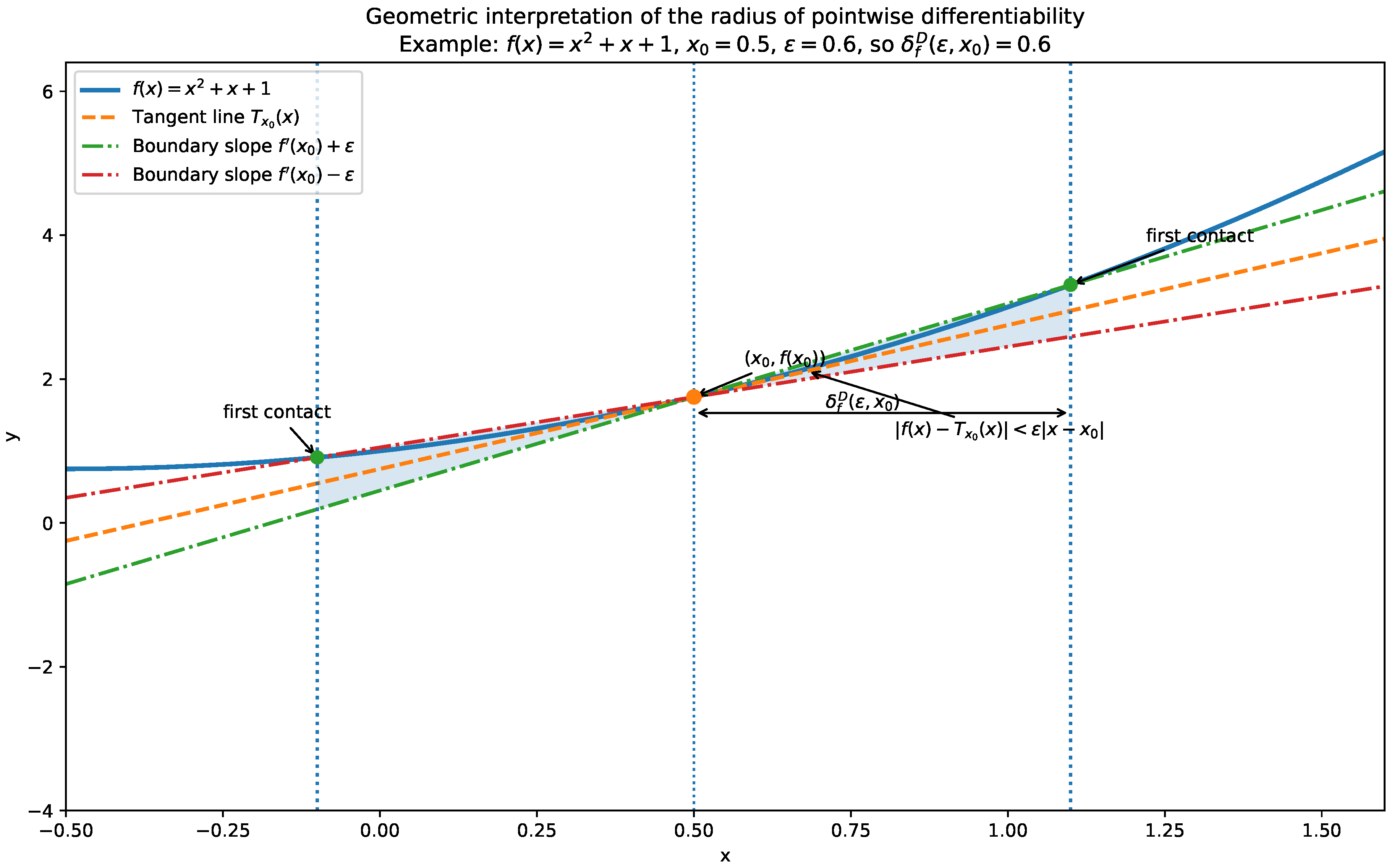
Geometric Interpretation (Pointwise)

Fix a differentiability point $x_0$. The tangent line $T_{x_0}$ is drawn at $(x_0,f\left(x_0\right))$, together with the two boundary lines of slopes $f^{\prime }\left(x_0\right)\pm \epsilon$. Admissible radii $\delta$ are those for which every secant line from $(x_0,f\left(x_0\right))$ to $(x,f(x\left)\right)$ with $0<|x-x_0|<\delta$ has slope within $\epsilon$ of $f^{\prime }\left(x_0\right)$. Equivalently, the graph remains inside the wedge

$$|f\left(x\right)-T_{x_0}\left(x\right)|<\epsilon |x-x_0|.$$

The maximal radius ${\delta }_f^D(\epsilon ,x_0)$ is attained at the first point where the graph touches or exits this wedge.

Figure 1. Geometric illustration of the pointwise radius of differentiability: Pointwise differentiability wedge at $x_0=\frac{1}{2}$ for $f\left(x\right)=x^2+x+1$ with $\epsilon =0.6$; the first boundary contact occurs at distance ${\delta }_f^D(\epsilon ,x_0)=0.6$.

Figure 1. Geometric illustration of the pointwise radius of differentiability: Pointwise differentiability wedge at $x_0=\frac{1}{2}$ for $f\left(x\right)=x^2+x+1$ with $\epsilon =0.6$; the first boundary contact occurs at distance ${\delta }_f^D(\epsilon ,x_0)=0.6$.

 Remark 2

(Shifted-h Formulation). For $x_0\in D\left(f\right)$ and $\delta >0$, define the pointwise differentiability oscillation by

$${\omega }_f^D(x_0;\delta ):=\underset{0<\left|h\right|<\delta }{sup}\left|{\displaystyle \frac{f(x_0+h)-f\left(x_0\right)}{h}}-f^{\prime }\left(x_0\right)\right|.$$

(11)

Then

$${\Delta }_f^D(\epsilon ,x_0)=\{\delta >0:{\omega }_f^D(x_0;\delta )<\epsilon \},$$

(12)

and

$${\delta }_f^D(\epsilon ,x_0)=sup\{\delta >0:{\omega }_f^D(x_0;\delta )<\epsilon \}.$$

(13)

 Remark 3

(Difference-Quotient Interpretation). Fix $x_0\in \mathbb{R}$, and define the difference-quotient map

$$Q_f(x;x_0):={\displaystyle \frac{f\left(x\right)-f\left(x_0\right)}{x-x_0}},x\in \mathbb{R}\setminus \left\{x_0\right\}.$$

Then, f is differentiable at $x_0$ if and only if the the extension ${\tilde{Q}}_f(x;x_0):=Q_f(x;x_0)1_{x\ne x_0}\left(x\right)\left(x\right)+f^{\prime }\left(x_0\right)1_{x=x_0}\left(x\right)$ is continuous at $x_0$. Moreover, for every $\epsilon >0$ and every $x_0\in D\left(f\right)$, ${\Delta }_f^D(\epsilon ,x_0)={\Delta }_{{\tilde{Q}}_f(·;x_0)}(\epsilon ,x_0).$ Consequently,

$${\delta }_f^D(\epsilon ,x_0)={\delta }_{{\tilde{Q}}_f(·;x_0)}(\epsilon ,x_0).$$

 Proposition 2

(Properties of Radius of Pointwise Differentiability). Let $f:\mathbb{R}\to \mathbb{R}$. Then, for $\epsilon >0$ and $x_0\in D\left(f\right)$, the radius ${\delta }_f^D(\epsilon ,x_0)$ has the following properties.

(A) Single-function properties.

(i)

Evenness. If f is even, then ${\delta }_f^D(\epsilon ,x_0)={\delta }_f^D(\epsilon ,-x_0).$

(ii)

Scaling. If $c\ne 0$, then ${\delta }_{cf}^D(\epsilon ,x_0)={\delta }_f^D\left({\displaystyle \frac{\epsilon }{\left|c\right|}},x_0\right);$ if $c=0$, then ${\delta }_{0·f}^D(\epsilon ,x_0)=+\infty .$

(iii)

Large-$\epsilon$ for bounded derivative. If f is differentiable on $\mathbb{R},$ $|f^{\prime }\left(x\right)|\le M$ for all $x\in \mathbb{R}$ and $\epsilon \ge 2M$, then ${\delta }_f^D(\epsilon ,x_0)=+\infty \mathrm{for}\mathrm{all}{x}_0\in \mathbb{R}.$

(iv)

Monotonicity in $\epsilon$. If $0<{\epsilon }_1\le {\epsilon }_2$, then ${\delta }_f^D({\epsilon }_1,x_0)\le {\delta }_f^D({\epsilon }_2,x_0).$

(v)

Input translation. If $g\left(x\right)=f(x+a)$, then ${\delta }_g^D(\epsilon ,x_0)={\delta }_f^D(\epsilon ,x_0+a).$

(vi)

Local derivative-control lower bound. If $f^{\prime }$ is L-Lipschitz on $|x-x_0|<r$ [13], then ${\delta }_f^D(\epsilon ,x_0)\ge min\left\{r,{\displaystyle \frac{2\epsilon }{L}}\right\}.$ In particular, if $f^{\prime }$ is globally L-Lipschitz on $\mathbb{R}$, then ${\delta }_f^D(\epsilon ,x_0)\ge {\displaystyle \frac{2\epsilon }{L}}.$

(vii)

Differentiability criterion. The function f is differentiable at $x_0$ iff ${\delta }_f^D(\epsilon ,x_0)>0\mathrm{for}\mathrm{every}\epsilon >0.$

(B) Two-function properties.

(viii)

Composition (one convenient bound). Assume f is differentiable at $x_0$, and assume that g is differentiable on $|u-f(x_0\left)\right|<\rho$ with $g^{\prime }$ being L-Lipschitz there. Set $B:=|f^{\prime }\left(x_0\right)|+1.$ Then, for any $\alpha \in [0,1]$,

$${\delta }_{g\circ f}^D(\epsilon ,x_0)\ge min\left\{{\delta }_f^D(1,x_0),{\displaystyle \frac{\rho }{B}},{\displaystyle \frac{\alpha \epsilon }{L{B}^2}},{\delta }_f^D\left({\displaystyle \frac{(1-\alpha )\epsilon }{|g^{\prime }\left(f\left(x_0\right)\right)|+1}},x_0\right)\right\}.$$

(ix)

Sum (lower bound). For $f_1,f_2$ and any $\alpha \in [0,1]$,

$${\delta }_{f_1+f_2}^D(\epsilon ,x_0)\ge min\left\{{\delta }_{f_1}^D(\alpha \epsilon ,x_0),{\delta }_{f_2}^D((1-\alpha )\epsilon ,x_0)\right\}.$$

(x)

Linear combination (lower bound). For $c_1,c_2\in \mathbb{R}$ and any $\alpha \in [0,1]$,

$${\delta }_{c_1{f}_1+c_2{f}_2}^D(\epsilon ,x_0)\ge min\left\{{\delta }_{f_1}^D\left({\displaystyle \frac{\alpha \epsilon }{|c_1|}},x_0\right),{\delta }_{f_2}^D\left({\displaystyle \frac{(1-\alpha )\epsilon }{|c_2|}},x_0\right)\right\},$$

with the convention from (ii) when one coefficient is 0.

(xi)

Product (one convenient bound). If $|f_1\left(x\right)|\le A$ on $|x-x_0|<r$, then

$${\delta }_{f_1{f}_2}^D(\epsilon ,x_0)\ge min\left\{r,{\delta }_{f_1}^D(1,x_0),{\delta }_{f_2}^D\left({\displaystyle \frac{\epsilon }{3A}},x_0\right),{\delta }_{f_1}^D\left({\displaystyle \frac{\epsilon }{3\left(\right|f_2\left(x_0\right)|+1)}},x_0\right),{\displaystyle \frac{\epsilon }{3\left(\right|f_2^{\prime }\left(x_0\right)|+1)\left(\right|f_1^{\prime }\left(x_0\right)|+1)}}\right\}.$$

Proof. 

The proof is divided according to the listed assertions. (i). If f is even, then $f^{\prime }$ is odd on $D\left(f\right)$, and with $k=-h$, $\left|Q_f(-x_0+h;-x_0)-f^{\prime }(-x_0)\right|=\left|Q_f(x_0+k;x_0)-f^{\prime }\left(x_0\right)\right|.$ Taking suprema over $0<\left|h\right|<\delta$ gives ${\omega }_f^D(-x_0;\delta )={\omega }_f^D(x_0;\delta ),$ hence ${\delta }_f^D(\epsilon ,-x_0)={\delta }_f^D(\epsilon ,x_0)$. (ii). For $c\ne 0$, $\left|Q_{cf}(x;x_0)-{\left(cf\right)}^{\prime }\left(x_0\right)\right|=\left|c\left(Q_f(x;x_0)-f^{\prime }\left(x_0\right)\right)\right|,$ yielding ${\omega }_{cf}^D(x_0;\delta )=\left|c\right|{\omega }_f^D(x_0;\delta ),$ so ${\omega }_{cf}^D(x_0;\delta )<\epsilon$ iff ${\omega }_f^D(x_0;\delta )<\epsilon /\left|c\right|$. Therefore ${\delta }_{cf}^D(\epsilon ,x_0)={\delta }_f^D\left({\displaystyle \frac{\epsilon }{\left|c\right|}},x_0\right).$ If $c=0$, then ${\omega }_{0·f}^D(x_0;\delta )=0$ for all $\delta >0$, hence ${\delta }_{0·f}^D(\epsilon ,x_0)=+\infty$. (iii). By the Mean Value Theorem, for each $x\ne x_0$ there exists $\xi$ between x and $x_0$ such that $Q_f(x;x_0)=f^{\prime }\left(\xi \right).$ Therefore $|Q_f(x;x_0)-f^{\prime }\left(x_0\right)|\le |f^{\prime }\left(\xi \right)|+|f^{\prime }\left(x_0\right)|\le 2M.$ Thus, if $\epsilon \ge 2M$, every $\delta >0$ is admissible, and hence ${\delta }_f^D(\epsilon ,x_0)=+\infty .$ (iv). ${\Delta }_f^D({\epsilon }_1,x_0)\subseteq {\Delta }_f^D({\epsilon }_2,x_0).$ (v). $Q_g(x;x_0)-g^{\prime }\left(x_0\right)=Q_f(x+a;x_0+a)-f^{\prime }(x_0+a),$ so ${\omega }_g^D(x_0;\delta )={\omega }_f^D(x_0+a;\delta ).$ (vi) Suppose $f^{\prime }$ is L-Lipschitz on $|x-x_0|<r$. Then, for $0<|x-x_0|<r$,

$$|Q_f(x;x_0)-f^{\prime }\left(x_0\right)|=|{\displaystyle \frac{1}{x-x_0}}{\int }_{x_0}^x\left(f^{\prime }\left(t\right)-f^{\prime }\left(x_0\right)\right)dt,|\le {\displaystyle \frac{L}{|x-x_0|}}{\int }_{x_0}^x|t-x_0|dt={\displaystyle \frac{L}{2}}|x-x_0|.$$

Hence ${\omega }_f^D(x_0;\delta )\le {\displaystyle \frac{L\delta }{2}}(0<\delta \le r),$ which implies ${\delta }_f^D(\epsilon ,x_0)\ge min\left\{r,{\displaystyle \frac{2\epsilon }{L}}\right\}.$ The global version is immediate. (vii) By above Remark 3.2, $f\mathrm{is}\mathrm{differentiable}\mathrm{at}{x}_0$ iff ${lim}_{\delta \downarrow 0}{\omega }_f^D(x_0;\delta )=0$ iff $\forall \epsilon >0:{\delta }_f^D(\epsilon ,x_0)>0.$ (viii). Let $u_0:=f\left(x_0\right)$ and assume $B:=|f^{\prime }\left(x_0\right)|+1$ and

$$0<|x-x_0|<min\left\{{\delta }_f^D(1,x_0),{\displaystyle \frac{\rho }{B}}\right\},$$

Then $|Q_f(x;x_0)-f^{\prime }\left(x_0\right)|<1$ yields $|Q_f(x;x_0)|\le B,$ and hence $|f\left(x\right)-f\left(x_0\right)|=|Q_f(x;x_0)\left|\right|x-x_0|\le B|x-x_0|<\rho .$ By the Mean Value Theorem applied to g on the interval between $f\left(x\right)$ and $f\left(x_0\right)$, there exists $\xi$ between $f\left(x\right)$ and $f\left(x_0\right)$ such that $Q_{g\circ f}(x;x_0)=g^{\prime }\left(\xi \right)Q_f(x;x_0).$ Therefore

$$\begin{array}{cc}\hfill |Q_{g\circ f}(x;x_0)-{(g\circ f)}^{\prime }\left(x_0\right)|& =|g^{\prime }\left(\xi \right)Q_f(x;x_0)-g^{\prime }\left(u_0\right)f^{\prime }\left(x_0\right)|\hfill \\ & \le |g^{\prime }\left(\xi \right)-g^{\prime }\left(u_0\right)\left|\right|Q_f(x;x_0)|+|g^{\prime }\left(u_0\right)\left|\right|Q_f(x;x_0)-f^{\prime }\left(x_0\right)|.\hfill \end{array}$$

Since $g^{\prime }$ is L-Lipschitz on $|u-u_0|<\rho$, $|g^{\prime }\left(\xi \right)-g^{\prime }\left(u_0\right)|\le L|\xi -u_0|\le L|f\left(x\right)-f\left(x_0\right)|\le LB|x-x_0|,$ hence $|g^{\prime }\left(\xi \right)-g^{\prime }\left(u_0\right)\left|\right|Q_f(x;x_0)|\le L{B}^2|x-x_0|.$ If, in addition,

$$|x-x_0|<{\displaystyle \frac{\alpha \epsilon }{L{B}^2}}$$

and

$$|Q_f(x;x_0)-f^{\prime }\left(x_0\right)|<{\displaystyle \frac{(1-\alpha )\epsilon }{|g^{\prime }\left(u_0\right)|+1}},$$

then

$$|Q_{g\circ f}(x;x_0)-{(g\circ f)}^{\prime }\left(x_0\right)|<\alpha \epsilon +(1-\alpha )\epsilon =\epsilon .$$

This proves the stated lower bound. (ix). Since $Q_{f_1+f_2}(x;x_0)-{(f_1+f_2)}^{\prime }\left(x_0\right)=\left(Q_{f_1}(x;x_0)-f_1^{\prime }\left(x_0\right)\right)+\left(Q_{f_2}(x;x_0)-f_2^{\prime }\left(x_0\right)\right),$ we obtain ${\omega }_{f_1+f_2}^D(x_0;\delta )\le {\omega }_{f_1}^D(x_0;\delta )+{\omega }_{f_2}^D(x_0;\delta ).$ Therefore, if ${\omega }_{f_1}^D(x_0;\delta )<\alpha \epsilon ,$ and ${\omega }_{f_2}^D(x_0;\delta )<(1-\alpha )\epsilon ,$ then ${\omega }_{f_1+f_2}^D(x_0;\delta )<\epsilon$, and hence the assertion follows. (x). Apply (ii) to $c_1{f}_1$ and $c_2{f}_2$, and then apply (ix) on its result. (xi) Assume $A>0$; if $A=0$, then $f_1\equiv 0$ near $x_0$ and the claim is trivial. For $x\ne x_0$,

$$Q_{f_1{f}_2}(x;x_0)-{\left(f_1{f}_2\right)}^{\prime }\left(x_0\right)=f_1\left(x\right)\left(Q_{f_2}(x;x_0)-f_2^{\prime }\left(x_0\right)\right)+f_2\left(x_0\right)\left(Q_{f_1}(x;x_0)-f_1^{\prime }\left(x_0\right)\right)+f_2^{\prime }\left(x_0\right)\left(f_1\left(x\right)-f_1\left(x_0\right)\right).$$

If $0<\delta <min\left\{r,{\delta }_{f_1}^D(1,x_0)\right\},$ then $|f_1\left(x\right)|\le A$ on $0<|x-x_0|<\delta$, and $|f_1\left(x\right)-f_1\left(x_0\right)|=|x-x_0\left|\right|Q_{f_1}(x;x_0)|\le \delta (|f_1^{\prime }\left(x_0\right)|+1).$ Hence ${\omega }_{f_1{f}_2}^D(x_0;\delta )\le A{\omega }_{f_2}^D(x_0;\delta )+\left(\right|f_2\left(x_0\right)|+1){\omega }_{f_1}^D(x_0;\delta )+\left(\right|f_2^{\prime }\left(x_0\right)|+1)\left(\right|f_1^{\prime }\left(x_0\right)|+1)\delta .$ Therefore, if the three terms on the right are each $<\epsilon /3$, then ${\omega }_{f_1{f}_2}^D(x_0;\delta )<\epsilon$, which yields the desired result. □

 Theorem 3

(Characterization of the Radius of Pointwise Differentiability). Let $f:\mathbb{R}\to \mathbb{R}$ be a real-valued function with $D\left(f\right)\ne ⌀$. Then the following two statements hold:

(i)

f is non-affine. ⇔ There is $x_0\in D\left(f\right)$ there exists $\epsilon >0$ such that ${\delta }_f^D(\epsilon ,x_0)<+\infty$.

(ii)

f is affine. ⇔ For every $x_0\in D\left(f\right)$ and every $\epsilon >0$, we have ${\delta }_f^D(\epsilon ,x_0)=+\infty$.

Proof. 

It is sufficient to prove (ii) as (i) is its logical equivalent. It is trivial that f is affine iff ${\tilde{Q}}_f(.;x_0)$ is constant. Now, by Theorem 1, ${\tilde{Q}}_f(.;x_0)$ is constant iff ${\delta }_{{\tilde{Q}}_f(·;x_0)}(\epsilon ,x_0)=+\infty$ for every $x_0\in D\left(f\right)$ and every $\epsilon >0$. But, by Remark 3${\delta }_{{\tilde{Q}}_f(·;x_0)}(\epsilon ,x_0)={\delta }_f^D(\epsilon ,x_0).$ This proves the assertion. □

3.2. Radius of Uniform Differentiability

We now pass from the local picture at a fixed base point to a global one. The purpose is to identify the largest single horizontal scale that makes the differentiability estimate work simultaneously throughout the entire domain.

 Definition 7

(Radius of Uniform Differentiability). Let $f:\mathbb{R}\to \mathbb{R}$ be a real-valued function differentiable on $\mathbb{R}$. For $\epsilon >0$, define the uniform admissible differentiability-radius set by

$${\Delta }_f^{UD}\left(\epsilon \right):=\left\{\delta >0:\forall x\in \mathbb{R},\forall h\in \mathbb{R},0<\left|h\right|<\delta ⟹\left|{\displaystyle \frac{f(x+h)-f\left(x\right)}{h}}-f^{\prime }\left(x\right)\right|<\epsilon \right\},$$

(14)

and define the radius of uniform differentiability by

$${\delta }_f^{UD}\left(\epsilon \right):=sup{\Delta }_f^{UD}\left(\epsilon \right).$$

(15)

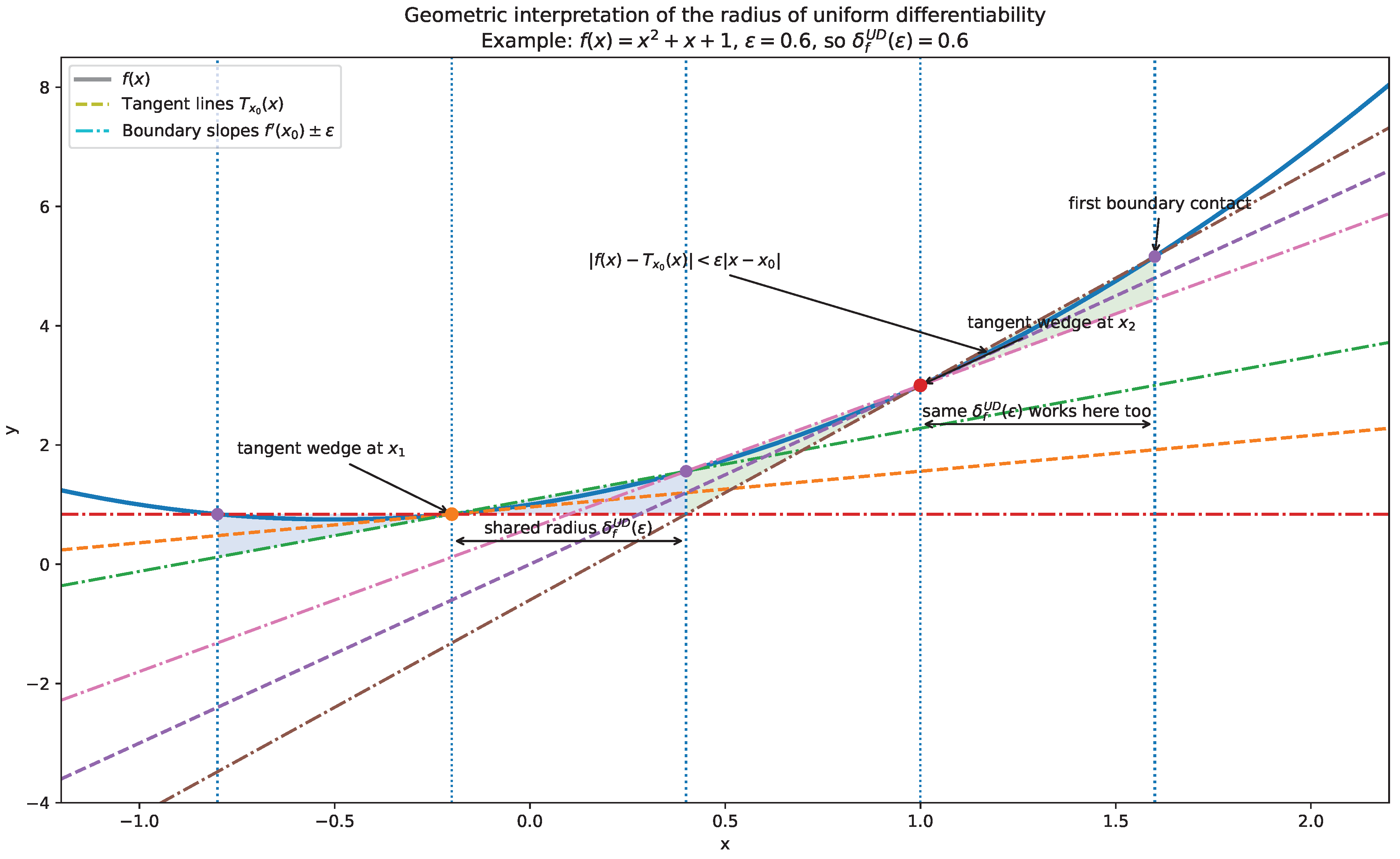
Geometric Interpretation (Uniform)

For each base point $x_0$, the graph of f is compared with its tangent line $T_{x_0}$. The admissible region is the wedge bounded by the two lines of slopes $f^{\prime }\left(x_0\right)\pm \epsilon$. A radius $\delta$ is admissible if, for every $x_0\in \mathbb{R}$, all secant lines from $(x_0,f\left(x_0\right))$ to nearby points $(x,f(x\left)\right)$ with $0<|x-x_0|<\delta$ have slope within $\epsilon$ of $f^{\prime }\left(x_0\right)$. Equivalently, the graph satisfies

$$|f\left(x\right)-T_{x_0}\left(x\right)|<\epsilon |x-x_0|.$$

The uniform radius ${\delta }_f^{UD}\left(\epsilon \right)$ is the largest common radius for which this holds simultaneously at every base point.

Figure 2. Geometric illustration of the uniform radius of differentiability: Uniform differentiability wedges for $f\left(x\right)=x^2+x+1$ with $\epsilon =0.6$; the common first boundary contact distance is ${\delta }_f^{UD}\left(\epsilon \right)=0.6$.

Figure 2. Geometric illustration of the uniform radius of differentiability: Uniform differentiability wedges for $f\left(x\right)=x^2+x+1$ with $\epsilon =0.6$; the common first boundary contact distance is ${\delta }_f^{UD}\left(\epsilon \right)=0.6$.

 Remark 4

(Shifted-h Formulation). Define the uniform differentiability oscillation by

$${\omega }_f^{UD}\left(\delta \right):=\underset{x\in \mathbb{R}}{sup}\underset{0<\left|h\right|<\delta }{sup}\left|{\displaystyle \frac{f(x+h)-f\left(x\right)}{h}}-f^{\prime }\left(x\right)\right|=\underset{x\in \mathbb{R}}{sup}\underset{0<\left|h\right|<\delta }{sup}\left|Q_f(x+h;x)-f^{\prime }\left(x\right)\right|.$$

(16)

Then

$${\Delta }_f^{UD}\left(\epsilon \right)=\{\delta >0:{\omega }_f^{UD}\left(\delta \right)<\epsilon \},$$

(17)

and

$${\delta }_f^{UD}\left(\epsilon \right)=sup\{\delta >0:{\omega }_f^{UD}\left(\delta \right)<\epsilon \}.$$

(18)

 Remark 5

(Uniform Difference-Quotient Profile Interpretation). Let $f:\mathbb{R}\to \mathbb{R}$ be differentiable on $\mathbb{R}$, and define the worst-case difference-quotient error profile by $r_f\left(h\right)={sup}_{x\in \mathbb{R}}\left|Q_f(x+h;x)-f^{\prime }\left(x\right)\right|1_{h\ne 0}\left(h\right),r_f\left(0\right)=0.$ Then, f is uniformly differentiable on $\mathbb{R}$ if and only if $r_f$ is continuous at 0. Moreover, for every $\epsilon >0$, ${\Delta }_f^{UD}\left(\epsilon \right)={\Delta }_{r_f}(\epsilon ,0).$ Consequently,

$${\delta }_f^{UD}\left(\epsilon \right)={\delta }_{r_f}(\epsilon ,0).$$

 Proposition 3

(Properties of Radius of Uniform Differentiability). Let $f:\mathbb{R}\to \mathbb{R}$ be differentiable on $\mathbb{R}$. Then, for $\epsilon >0$, the radius of uniform differentiability ${\delta }_f^{UD}\left(\epsilon \right)$ has the following properties.

(A) Single-function properties.

(i)

Scaling. If $c\ne 0$, then ${\delta }_{cf}^{UD}\left(\epsilon \right)={\delta }_f^{UD}\left({\displaystyle \frac{\epsilon }{\left|c\right|}}\right);$ if $c=0$, then ${\delta }_{0·f}^{UD}\left(\epsilon \right)=+\infty .$

(ii)

Monotonicity in $\epsilon$. If $0<{\epsilon }_1\le {\epsilon }_2$, then ${\delta }_f^{UD}\left({\epsilon }_1\right)\le {\delta }_f^{UD}\left({\epsilon }_2\right).$

(iii)

Translation/reflection invariance. If $g\left(x\right)=f(x+a)$ or $g\left(x\right)=f(-x)$, then ${\delta }_g^{UD}\left(\epsilon \right)={\delta }_f^{UD}\left(\epsilon \right).$

(iv)

Large-$\epsilon$ for bounded derivative. If $|f^{\prime }\left(x\right)|\le M$ everywhere and $\epsilon >2M$, then ${\delta }_f^{UD}\left(\epsilon \right)=+\infty .$

(v)

Lipschitz lower bound on the derivative. If $f^{\prime }$ is globally L-Lipschitz on $\mathbb{R}$, then ${\delta }_f^{UD}\left(\epsilon \right)\ge {\displaystyle \frac{2\epsilon }{L}}.$

(vi)

Uniform differentiability criterion. The function f is uniformly differentiable on $\mathbb{R}$ iff ${\delta }_f^{UD}\left(\epsilon \right)>0\mathrm{for}\mathrm{all}\epsilon >0.$

(vii)

Link to pointwise differentiability radii. ${\delta }_f^{UD}\left(\epsilon \right)\le \underset{x\in \mathbb{R}}{inf}{\delta }_f^D(\epsilon ,x).$

(B) Two-function properties.

(viii)

Composition. Assume $|f^{\prime }\left(x\right)|\le B$ and $|g^{\prime }\left(u\right)|\le M$ on $\mathbb{R}$, with $B,M>0$, and assume that $g^{\prime }$ admits a global modulus η, that is, $|u-v|<\eta \left(\tau \right)⟹|g^{\prime }\left(u\right)-g^{\prime }\left(v\right)|<\tau .$ Then, for any $\alpha \in [0,1]$,

$${\delta }_{g\circ f}^{UD}\left(\epsilon \right)\ge min\left\{{\displaystyle \frac{\eta (\alpha \epsilon /B)}{B}},{\delta }_f^{UD}\left({\displaystyle \frac{(1-\alpha )\epsilon }{M}}\right)\right\}.$$

(ix)

Sum (lower bound). For $f_1,f_2$ and any $\alpha \in [0,1]$,

$${\delta }_{f_1+f_2}^{UD}\left(\epsilon \right)\ge min\left\{{\delta }_{f_1}^{UD}\left(\alpha \epsilon \right),{\delta }_{f_2}^{UD}\left((1-\alpha )\epsilon \right)\right\}.$$

There is no universal matching upper bound; for example, one may take $f_1=g$ and $f_2=-g$.

(x)

Linear combination (lower bound). For $c_1,c_2\in \mathbb{R}$ and any $\alpha \in [0,1]$,

$${\delta }_{c_1{f}_1+c_2{f}_2}^{UD}\left(\epsilon \right)\ge min\left\{{\delta }_{f_1}^{UD}\left({\displaystyle \frac{\alpha \epsilon }{|c_1|}}\right),{\delta }_{f_2}^{UD}\left({\displaystyle \frac{(1-\alpha )\epsilon }{|c_2|}}\right)\right\},$$

with the convention from (i) when a coefficient is 0.

(xi)

Product (one convenient global bound). If $|f_1\left(x\right)|\le A$, $|f_2\left(x\right)|\le B$, $|f_1^{\prime }\left(x\right)|\le C_1$, and $|f_2^{\prime }\left(x\right)|\le C_2$ on $\mathbb{R}$, with $A,B,C_1,C_2>0$, then for any $\alpha ,\beta \ge 0$ with $\alpha +\beta \le 1$,

$${\delta }_{f_1{f}_2}^{UD}\left(\epsilon \right)\ge min\left\{{\delta }_{f_2}^{UD}\left({\displaystyle \frac{\alpha \epsilon }{A}}\right),{\delta }_{f_1}^{UD}\left({\displaystyle \frac{\beta \epsilon }{B}}\right),{\displaystyle \frac{(1-\alpha -\beta )\epsilon }{C_1{C}_2}}\right\}.$$

Proof. 

The proof is divided according to the listed assertions. (i). $|Q_{cf}(x+h;x)-{\left(cf\right)}^{\prime }\left(x\right)|=|c\left(Q_f(x+h;x)-f^{\prime }\left(x\right)\right)|,$ hence ${\omega }_{cf}^{UD}\left(\delta \right)=\left|c\right|{\omega }_f^{UD}\left(\delta \right).$ If $c=0$, then the oscillation is identically zero. (ii). Given $0<{\epsilon }_1\le {\epsilon }_2$ we have ${\Delta }_f^{UD}\left({\epsilon }_1\right)\le {\Delta }_f^{UD}\left({\epsilon }_2\right).$ Taking suprema yields the result. (iii). If $g\left(x\right)=f(x+a)$, then $Q_g(x+h;x)-g^{\prime }\left(x\right)=Q_f(x+h+a;x+a)-f^{\prime }(x+a),$ so the corresponding oscillations agree. If $g\left(x\right)=f(-x)$, then $Q_g(x+h;x)-g^{\prime }\left(x\right)=-(Q_f(-x-h;-h)-f^{\prime }(-x))$ and taking absolute values and suprema again yields the same oscillation. (iv). By the Mean Value Theorem, for each $x\in \mathbb{R}$ and $h\ne 0$, there exists $\xi$ between x and $x+h$ such that $Q_f(x+h;x)=f^{\prime }\left(\xi \right).$ Therefore $|Q_f(x+h;x)-f^{\prime }\left(x\right)|\le |f^{\prime }\left(\xi \right)|+|f^{\prime }\left(x\right)|\le 2M.$ Hence, if $\epsilon >2M$, every $\delta >0$ is admissible, so the assertion follows. (v). Since $f^{\prime }$ is globally L-Lipschitz, for every $x\in \mathbb{R}$ and $h\ne 0$,

$$|Q_f(x+h;x)-f^{\prime }\left(x\right)|=|{\displaystyle \frac{1}{h}}{\int }_0^h\left(f^{\prime }(x+t)-f^{\prime }\left(x\right)\right)dt|\le {\displaystyle \frac{1}{\left|h\right|}}{\int }_0^{\left|h\right|}Ltdt={\displaystyle \frac{L}{2}}\left|h\right|.$$

Thus every $\delta \le {\displaystyle \frac{2\epsilon }{L}}$ is admissible or ${\omega }_f^{UD}\left(\delta \right)\le {\displaystyle \frac{2\epsilon }{L}}.$ (vi). This is exactly the $\epsilon -\delta$ definition of uniform differentiability. (vii). If $\delta \in {\Delta }_f^{UD}\left(\epsilon \right)$ then, fixing any $x_0$, $|x-x_0|<\delta$ yields $|Q_f(x;x_0)-f^{\prime }\left(x_0\right)|<\epsilon$, hence $\delta \in {\Delta }_f^D(\epsilon ,x_0)$; take sups and then the infimum over $x_0$. (viii). Let $h\ne 0$. By the chain rule, ${(g\circ f)}^{\prime }\left(x\right)=g^{\prime }\left(f\left(x\right)\right)f^{\prime }\left(x\right),$ and

$Q_{g\circ f}(x+h;x)-g^{\prime }\left(f\left(x\right)\right)f^{\prime }\left(x\right)=(Q_g(f(x+h);f\left(x\right))-g^{\prime }\left(f\left(x\right)\right))Q_f(x+h;x)+g^{\prime }\left(f\left(x\right)\right)(Q_f(x+h;x)-f^{\prime }\left(x\right)).$ Since $|f^{\prime }|\le B$, the Mean Value Theorem gives $|Q_f(x+h;x)|\le B\mathrm{and}|f(x+h)-f\left(x\right)|\le B|h|.$ Thus, if

$$\left|h\right|<{\displaystyle \frac{\eta (\alpha \epsilon /B)}{B}},$$

then $\left|f\right(x+h)-f(x\left)\right|<\eta (\alpha \epsilon /B),$ and hence $|(Q_g(f(x+h);f\left(x\right))-g^{\prime }\left(f\left(x\right)\right))|<{\displaystyle \frac{\alpha \epsilon }{B}}.$ Multiplying by $|Q_f(x+h;x)|\le B$ yields a contribution $<\alpha \epsilon$. Also, if

$$\left|h\right|<{\delta }_f^{UD}\left({\displaystyle \frac{(1-\alpha )\epsilon }{M}}\right),$$

then $|Q_f(x+h;x)-f^{\prime }\left(x\right)|<{\displaystyle \frac{(1-\alpha )\epsilon }{M}},$ so $|g^{\prime }\left(f\left(x\right)\right)\left|\right|Q_f(x+h;x)-f^{\prime }\left(x\right)|<(1-\alpha )\epsilon .$ Summing the two bounds proves the claim. (ix). Given, $Q_{f_1+f_2}(x+h;x)-{(f_1+f_2)}^{\prime }\left(x\right)=\left(Q_{f_1}(x+h;x)-f_1^{\prime }\left(x\right)\right)+\left(Q_{f_2}(x+h;x)-f_2^{\prime }\left(x\right)\right).$ Now, applying the triangle inequality and splitting $\epsilon$ into $\alpha \epsilon$ and $(1-\alpha )\epsilon$ gives the stated lower bound. (x). Apply (i) to $c_1{f}_1$ and $c_2{f}_2$, and then apply (ix) to obtain the plausible assertion. (xi). For $h\ne 0$, $Q_{f_1{f}_2}(x+h;x)=f_1(x+h)Q_{f_2}(x+h;x)+f_2\left(x\right)Q_{f_1}(x+h;x).$ Subtracting ${\left(f_1{f}_2\right)}^{\prime }\left(x\right)=f_1^{\prime }\left(x\right)f_2\left(x\right)+f_1\left(x\right)f_2^{\prime }\left(x\right)$ yields

$$\begin{array}{cc}\hfill Q_{f_1{f}_2}(x+h;x)-{\left(f_1{f}_2\right)}^{\prime }\left(x\right)& =f_1(x+h)\left(Q_{f_2}(x+h;x)-f_2^{\prime }\left(x\right)\right)\hfill \\ & +f_2\left(x\right)\left(Q_{f_1}(x+h;x)-f_1^{\prime }\left(x\right)\right)\hfill \\ & +f_2^{\prime }\left(x\right)\left(f_1(x+h)-f_1\left(x\right)\right).\hfill \end{array}$$

Now $|f_1(x+h)|\le A$, $|f_2\left(x\right)|\le B$, and by the Mean Value Theorem, $|f_1(x+h)-f_1\left(x\right)|\le C_1\left|h\right|.$ Hence, if

$$\left|h\right|<{\delta }_{f_2}^{UD}\left({\displaystyle \frac{\alpha \epsilon }{A}}\right),\left|h\right|<{\delta }_{f_1}^{UD}\left({\displaystyle \frac{\beta \epsilon }{B}}\right),\left|h\right|<{\displaystyle \frac{(1-\alpha -\beta )\epsilon }{C_1{C}_2}},$$

then the three terms are bounded respectively by $\alpha \epsilon ,\beta \epsilon ,(1-\alpha -\beta )\epsilon ,$ respectively. Adding them gives $|Q_{f_1{f}_2}(x+h;x)-{\left(f_1{f}_2\right)}^{\prime }\left(x\right)|<\epsilon ,$ which proves the result. □

 Theorem 4

(Characterization of the Radius of Uniform Differentiability). Let $f:\mathbb{R}\to \mathbb{R}$ be differentiable on $\mathbb{R}$. Then the following two statements hold:

(i)

f is non-affine on $\mathbb{R}$. ⇔ There exists $\epsilon >0$ such that ${\delta }_f^{UD}\left(\epsilon \right)<+\infty .$

(ii)

f is affine on $\mathbb{R}$. ⇔ For every $\epsilon >0$, one has ${\delta }_f^{UD}\left(\epsilon \right)=+\infty .$

Proof. 

It is sufficient to prove (ii) as (i) is its logical equivalent. We provide two proofs for (ii).

• Proof(1) for (ii)

It is trivial that f is affine iff $r_f$ vanishes identically. Next, by Theorem 1, and the definition of $r_f$ in the Remark 5, $r_f$ is constant zero (and poinswise continuous at $x_0=0$) iff ${\delta }_{r_f}(\epsilon ,0)=+\infty$ for every $\epsilon >0$. But, by Remark 5, ${\delta }_{r_f}(\epsilon ,0)={\delta }_f^{UD}\left(\epsilon \right)$ for every $\epsilon >0.$ This completes the proof.

• Proof(2) for (ii)

Assume first that f is affine on $\mathbb{R}$. Since f is differentiable on $\mathbb{R}$, we have $D\left(f\right)=\mathbb{R}$. Hence, by Theorem 3(ii), for every $x\in \mathbb{R}$ and every $\epsilon >0$, we have ${\delta }_f^D(\epsilon ,x)=+\infty .$ Therefore, for every $\epsilon >0$, we have ${inf}_{x\in \mathbb{R}}{\delta }_f^D(\epsilon ,x)=+\infty .$ Applying Proposition 4, for every $\epsilon >0$, we obtain ${\delta }_f^{UD}\left(\epsilon \right)={inf}_{x\in \mathbb{R}}{\delta }_f^D(\epsilon ,x)=+\infty .$

Conversely, assume that for every $\epsilon >0$, we have ${\delta }_f^{UD}\left(\epsilon \right)=+\infty .$ Suppose, toward a contradiction, that f is non-affine on $\mathbb{R}$. Then, by Theorem 3(i), there exist $x_0\in D\left(f\right)=\mathbb{R}$ and ${\epsilon }_0>0$ such that ${\delta }_f^D({\epsilon }_0,x_0)<+\infty .$ Now Proposition 4 yields ${\delta }_f^{UD}\left({\epsilon }_0\right)={inf}_{x\in \mathbb{R}}{\delta }_f^D({\epsilon }_0,x)\le {\delta }_f^D({\epsilon }_0,x_0)<+\infty ,$ which contradicts the original assumption. Hence f must be affine on $\mathbb{R}$.

□

3.3. Connection Between the Pointwise and Uniform Radii of Differentiability

The pointwise and uniform radii introduced above are local and global versions of the same quantitative phenomenon. We now clarify their precise relationship.

Lemma 1 (Downward Closedness of Admissible Radius Sets). Let $f:\mathbb{R}\to \mathbb{R}$, let $\epsilon >0$, and let $x_0\in D\left(f\right)$. Then

$$\delta \in {\Delta }_f^D(\epsilon ,x_0),0<\eta \le \delta ⟹\eta \in {\Delta }_f^D(\epsilon ,x_0),$$

(19)

and

$$\delta \in {\Delta }_f^{UD}\left(\epsilon \right),0<\eta \le \delta ⟹\eta \in {\Delta }_f^{UD}\left(\epsilon \right).$$

(20)

In particular, both admissible-radius sets are downward closed.

Proof. Suppose $\delta \in {\Delta }_f^D(\epsilon ,x_0)$ and $0<\eta \le \delta$. If $0<|x-x_0|<\eta$, then automatically $0<|x-x_0|<\delta$. Since $\delta$ is admissible, it follows that $\left|Q_f(x;x_0)-f^{\prime }\left(x_0\right)\right|<\epsilon .$ Hence $\eta \in {\Delta }_f^D(\epsilon ,x_0)$, proving (19).

The proof of (20) is identical. Suppose $\delta \in {\Delta }_f^{UD}\left(\epsilon \right)$ and $0<\eta \le \delta$. If $0<\left|h\right|<\eta$, then $0<\left|h\right|<\delta$, and therefore for every $x\in \mathbb{R}$, we have $\left|Q_f(x+h;x)-f^{\prime }\left(x\right)\right|<\epsilon .$ Thus $\eta \in {\Delta }_f^{UD}\left(\epsilon \right)$. □

Lemma 2 (Uniform Admissible Radius as an Intersection). Let $f:\mathbb{R}\to \mathbb{R}$ be differentiable on $\mathbb{R}$, and let $\epsilon >0$. Then

$${\Delta }_f^{UD}\left(\epsilon \right)=\bigcap _{x\in \mathbb{R}}{\Delta }_f^D(\epsilon ,x).$$

(21)

Proof. First, let $\delta \in {\Delta }_f^{UD}\left(\epsilon \right)$. Then by definition, for all $x\in \mathbb{R}$ and all $h\in \mathbb{R}$, whenever $0<\left|h\right|<\delta$ we have $\left|Q_f(x+h;x)-f^{\prime }\left(x\right)\right|<\epsilon .$ Fix any $x_0\in \mathbb{R}$. If $0<|x-x_0|<\delta$, then setting $h=x-x_0$ gives $\left|Q_f(x;x_0)-f^{\prime }\left(x_0\right)\right|<\epsilon ,$ which shows that $\delta \in {\Delta }_f^D(\epsilon ,x_0)$. Since $x_0$ was arbitrary, we have $\delta \in {\bigcap }_{x\in \mathbb{R}}{\Delta }_f^D(\epsilon ,x).$ Therefore

$${\Delta }_f^{UD}\left(\epsilon \right)\subseteq \bigcap _{x\in \mathbb{R}}{\Delta }_f^D(\epsilon ,x).$$

(22)

Conversely, let $\delta \in {\bigcap }_{x\in \mathbb{R}}{\Delta }_f^D(\epsilon ,x).$ Then for every $x\in \mathbb{R}$ we have $\delta \in {\Delta }_f^D(\epsilon ,x)$. Now take arbitrary $x\in \mathbb{R}$ and $h\in \mathbb{R}$ with $0<\left|h\right|<\delta$. Since $\delta \in {\Delta }_f^D(\epsilon ,x)$, choosing $x+h$ in the role of the nearby point gives $\left|Q_f(x+h;x)-f^{\prime }\left(x\right)\right|<\epsilon .$ Hence $\delta \in {\Delta }_f^{UD}\left(\epsilon \right)$. Therefore

$$\bigcap _{x\in \mathbb{R}}{\Delta }_f^D(\epsilon ,x)\subseteq {\Delta }_f^{UD}\left(\epsilon \right).$$

(23)

Combining (22) and (23), we obtain (21). □

Proposition 4 (Uniform Radius as the Infimum of the Pointwise Radii). Let $f:\mathbb{R}\to \mathbb{R}$ be differentiable on $\mathbb{R}$, and let $\epsilon >0$. Then

$${\delta }_f^{UD}\left(\epsilon \right)=\underset{x\in \mathbb{R}}{inf}{\delta }_f^D(\epsilon ,x).$$

(24)

In particular, the radius of uniform differentiability is the global bottleneck among the pointwise differentiability radii.

Proof. By Lemma 2, we have ${\Delta }_f^{UD}\left(\epsilon \right)={\bigcap }_{x\in \mathbb{R}}{\Delta }_f^D(\epsilon ,x).$ Hence, for every $x\in \mathbb{R}$, we have ${\Delta }_f^{UD}\left(\epsilon \right)\subseteq {\Delta }_f^D(\epsilon ,x).$ Next, taking suprema in both sides, we obtain ${\delta }_f^{UD}\left(\epsilon \right)\le {\delta }_f^D(\epsilon ,x)(x\in \mathbb{R}),$ and therefore

$${\delta }_f^{UD}\left(\epsilon \right)\le \underset{x\in \mathbb{R}}{inf}{\delta }_f^D(\epsilon ,x).$$

(25)

For the reverse inequality, set $\alpha :={inf}_{x\in \mathbb{R}}{\delta }_f^D(\epsilon ,x).$ Let $0<\eta <\alpha$. Then for every $x\in \mathbb{R}$, we have $\eta <{\delta }_f^D(\epsilon ,x)=sup{\Delta }_f^D(\epsilon ,x).$ Since f is differentiable on $\mathbb{R}$, each set ${\Delta }_f^D(\epsilon ,x)$ is nonempty. Hence for every $x\in \mathbb{R}$ there exists ${\delta }_x\in {\Delta }_f^D(\epsilon ,x)$ such that $\eta <{\delta }_x$. By Lemma 1, the set ${\Delta }_f^D(\epsilon ,x)$ is downward closed, so from ${\delta }_x\in {\Delta }_f^D(\epsilon ,x)$ and $0<\eta <{\delta }_x$ we conclude that $\eta \in {\Delta }_f^D(\epsilon ,x)(x\in \mathbb{R}).$ Therefore, $\eta \in {\bigcap }_{x\in \mathbb{R}}{\Delta }_f^D(\epsilon ,x)={\Delta }_f^{UD}\left(\epsilon \right),$ by Lemma 2. Since this holds for every $0<\eta <\alpha$, we obtain

$${\delta }_f^{UD}\left(\epsilon \right)=sup{\Delta }_f^{UD}\left(\epsilon \right)\ge \alpha =\underset{x\in \mathbb{R}}{inf}{\delta }_f^D(\epsilon ,x).$$

(26)

Combining (25) and (26) completes the proof. □

Corollary 1 (Consequences of the bottleneck identity). Let $f:\mathbb{R}\to \mathbb{R}$ be differentiable on $\mathbb{R}$, and let $\epsilon >0$. Then the following statements hold.

(i)

If there exist ${\epsilon }_0>0$ and a sequence ${\left(x_n\right)}_{n\ge 1}\subseteq \mathbb{R}$ such that

$${\delta }_f^D({\epsilon }_0,x_n)⟶0,$$

(27)

then

$${\delta }_f^{UD}\left({\epsilon }_0\right)=0,$$

(28)

and consequently f is not uniformly differentiable on $\mathbb{R}$.

(ii)

If for every $\epsilon >0$ there exists a positive function $m_D\left(\epsilon \right)$ such that

$${\delta }_f^D(\epsilon ,x)\ge m_D\left(\epsilon \right)\mathrm{for}\mathrm{all}x\in \mathbb{R},$$

(29)

then

$${\delta }_f^{UD}\left(\epsilon \right)\ge m_D\left(\epsilon \right)\mathrm{for}\mathrm{all}\epsilon >0,$$

(30)

and hence f is uniformly differentiable on $\mathbb{R}$.

(iii)

If for some $\epsilon >0$ there exists $x_{*}\in \mathbb{R}$ such that

$${\delta }_f^D(\epsilon ,x_{*})=\underset{x\in \mathbb{R}}{inf}{\delta }_f^D(\epsilon ,x),$$

(31)

then

$${\delta }_f^{UD}\left(\epsilon \right)={\delta }_f^D(\epsilon ,x_{*}).$$

(32)

In this situation, the point $x_{*}$ may be interpreted as a differentiability bottleneck at scale ε: the local first-order approximation of f at $x_{*}$ determines the global uniform differentiability radius.

(iv)

Whenever the map $x\mapsto {\delta }_f^D(\epsilon ,x)$ is available in explicit form, the corresponding uniform radius may be recovered from the one-dimensional optimization formula

$${\delta }_f^{UD}\left(\epsilon \right)=\underset{x\in \mathbb{R}}{inf}{\delta }_f^D(\epsilon ,x).$$

(33)

Thus the global problem of finding a single admissible differentiability radius reduces to minimizing the pointwise differentiability radius over the base point.

Proof. Each claim follows directly from Proposition 4. Indeed, parts (i), (ii), and (iv) are obtained by taking the infimum of the family $\{{\delta }_f^D(\epsilon ,x):x\in \mathbb{R}\}$, while part (iii) corresponds to the special case in which that infimum is attained at a point $x_{*}$. □

Example 2 (Application of part (i): detecting failure of uniform differentiability). Let $f\left(x\right)=x^3$. Fix $\epsilon >0$ and a base point $x_0\in \mathbb{R}$. For $h\ne 0$ and $\left|h\right|<\delta$, we have $\left|Q_f(x_0+h;x_0)-f^{\prime }\left(x_0\right)\right|=|3x_{0}h+h^2|\le \delta (3|x_0|+\delta ).$ Therefore every $\delta >0$ satisfying $\delta \left(3\right|x_0|+\delta )<\epsilon$ is admissible, and the maximal one is ${\delta }_f^D(\epsilon ,x_0)={\displaystyle \frac{2\epsilon }{\sqrt{9x_0^2+4\epsilon }+3\left|x_0\right|}}.$ Now choose $x_n=n$. Then ${\delta }_f^D(\epsilon ,n)⟶0.$ By part (i), we have ${\delta }_f^{UD}\left(\epsilon \right)=0,$ so $x^3$ is not uniformly differentiable on $\mathbb{R}$.

Example 3 (Application of part (ii): proving uniform differentiability from a global lower bound). Let $f\left(x\right)=sinx$. For $h\ne 0$, we have $Q_f(x+h;x)-f^{\prime }\left(x\right)={\displaystyle \frac{1}{h}}{\int }_0^h\left(cos(x+t)-cosx\right)dt.$ Since $|cos(x+t)-cosx|\le \left|t\right|$ for all $x,t\in \mathbb{R}$, it follows that $\left|Q_f(x+h;x)-f^{\prime }\left(x\right)\right|\le {\displaystyle \frac{1}{\left|h\right|}}{\int }_0^{\left|h\right|}tdt={\displaystyle \frac{\left|h\right|}{2}}.$ Consequently, every $\delta \le 2\epsilon$ is admissible at every base point x, and hence ${\delta }_f^D(\epsilon ,x)\ge 2\epsilon \mathrm{for}\mathrm{all}x\in \mathbb{R}.$ Part (ii) now yields ${\delta }_f^{UD}\left(\epsilon \right)\ge 2\epsilon >0,$ which shows that $sinx$ is uniformly differentiable on $\mathbb{R}$.

Example 4 (Application of part (iii): a bottleneck point may be attained, and need not be unique). Let $f\left(x\right)=x^2$. Then for every $x\in \mathbb{R}$ and every $h\ne 0$, we have $\left|Q_f(x+h;x)-f^{\prime }\left(x\right)\right|=\left|h\right|<\epsilon$ precisely when $\left|h\right|<\epsilon$. Therefore ${\delta }_f^D(\epsilon ,x)=\epsilon \mathrm{for}\mathrm{all}x\in \mathbb{R}.$ Hence the infimum is attained at every base point; in particular, one may take $x_{*}=0$. By part (iii), we have ${\delta }_f^{UD}\left(\epsilon \right)={\delta }_f^D(\epsilon ,0)=\epsilon .$ So, in this case, the differentiability bottleneck is completely flat: no single point is more restrictive than another.

Example 5 (Application of part (iv): computing the uniform radius from an explicit pointwise formula). Let $f\left(x\right)=\frac{1}{2}{x}^2+x$. Then $f^{\prime }\left(x\right)=x+1$, and for every $x\in \mathbb{R}$ and $h\ne 0$, we have $\left|Q_f(x+h;x)-f^{\prime }\left(x\right)\right|={\displaystyle \frac{\left|h\right|}{2}}<\epsilon$ if and only if $\left|h\right|<2\epsilon$. Hence the pointwise differentiability radius is explicitly given by ${\delta }_f^D(\epsilon ,x)=2\epsilon \mathrm{for}\mathrm{all}x\in \mathbb{R}.$ Applying part (iv), we obtain ${\delta }_f^{UD}\left(\epsilon \right)={inf}_{x\in \mathbb{R}}{\delta }_f^D(\epsilon ,x)=2\epsilon .$ Thus the global uniform radius is recovered immediately by minimizing the explicit pointwise formula.

3.4. Connection Between the Radius of Differentiability and the Radius of Continuity

The radii of continuity and differentiability introduced in previous paper and this paper are associated for specific classes of the functions.

Proposition 5 (Pointwise differentiability radius of the antiderivative). Let $f:[a,b]\to \mathbb{R}$ be continuous, and define

$$F\left(x\right):={\int }_a^{x}f\left(t\right)dt,x\in [a,b].$$

(i)

${\delta }_F^D(\epsilon ,x_0)\ge {\delta }_f(\epsilon ,x_0):$ for every $\epsilon >0,x_0\in (a,b).$

(ii)

${\delta }_F^{UD}\left(\epsilon \right)\ge {\delta }_f^U\left(\epsilon \right):$ for every $\epsilon >0.$

Proof. The proof is divided according to the listed assertions. (i). Fix $x_0\in (a,b)$ and $\epsilon >0$. Take any $x\in [a,b]$ with $0<|x-x_0|<\delta$. By the Fundamental Theorem of Calculus,

$$F^{\prime }\left(x_0\right)=f\left(x_0\right),F\left(x\right)-F\left(x_0\right)={\int }_{x_0}^{x}f\left(t\right)dt.$$

Hence:

$$|Q_F(x;x_0)-F^{\prime }\left(x_0\right)|=|{\displaystyle \frac{1}{x-x_0}}{\int }_{x_0}^x\left(f\left(t\right)-f\left(x_0\right)\right)dt|\le {\displaystyle \frac{1}{|x-x_0|}}{\int }_{x_0}^x|f\left(t\right)-f\left(x_0\right)|dt.$$

(34)

Now every point t between $x_0$ and x satisfies $|t-x_0|\le |x-x_0|<\delta .$ Since $\delta \in {\Delta }_f(\epsilon ,x_0)$, we have $|f\left(t\right)-f\left(x_0\right)|<\epsilon \mathrm{for}\mathrm{all}t\mathrm{between}{x}_0\mathrm{and}x.$ Thus

$$\left|Q_F(x;x_0)-F^{\prime }\left(x_0\right)\right|<{\displaystyle \frac{1}{|x-x_0|}}{\int }_{x_0}^x\epsilon dt=\epsilon .$$

(35)

So $\delta \in {\Delta }_F^D(\epsilon ,x_0)$, proving ${\Delta }_f(\epsilon ,x_0)\subseteq {\Delta }_F^D(\epsilon ,x_0).$ Taking suprema yields the plausible result. (ii). There are two proofs for this part.

• Proof(1) for (ii)

This is indeed parallel to the proof in (i). Again, by the Fundamental Theorem of Calculus, and similar arguments on integral inequalities as in part (i), for any $\delta \in {\Delta }_f^U\left(\epsilon \right)$, we have $\delta \in {\Delta }_F^{UD}\left(\epsilon \right)$, proving ${\Delta }_f^U\left(\epsilon \right)\subseteq {\Delta }_F^{UD}\left(\epsilon \right),$$\mathrm{for}\mathrm{all}\epsilon >0.$ Taking suprema yields the plausible result.

• Proof(2) for (ii)

By part(i), ${\delta }_F^D(\epsilon ,x)\ge {\delta }_f(\epsilon ,x)$ for every $x\in (a,b)$; hence, taking infima over $x\in (a,b)$, we obtain ${inf}_{x\in (a,b)}{\delta }_F^D(\epsilon ,x)\ge {inf}_{x\in (a,b)}{\delta }_f(\epsilon ,x)$. Using the infimum characterizations of the uniform radii in Proposition 1 and Proposition 4, it follows that

$${\delta }_F^{UD}\left(\epsilon \right)=\underset{x\in (a,b)}{inf}{\delta }_F^D(\epsilon ,x)\ge \underset{x\in (a,b)}{inf}{\delta }_f(\epsilon ,x)={\delta }_f^U\left(\epsilon \right),$$

$\mathrm{for}\mathrm{all}\epsilon >0,$ as claimed. □

Remark 6. In general, the inequalities above are not equalities. For example, on $[0,1]$, let $f\left(x\right)=x$. Then $F\left(x\right)={\int }_0^{x}tdt={\displaystyle \frac{x^2}{2}}.$ Fix $x_0={\displaystyle \frac{1}{2}}$. For $0<\epsilon <{\displaystyle \frac{1}{4}}$, one has ${\delta }_f(\epsilon ,x_0)=\epsilon ,$ whereas $Q_F(x;x_0)-F^{\prime }\left(x_0\right)={\displaystyle \frac{x-x_0}{2}},$ so ${\delta }_F^D(\epsilon ,x_0)=2\epsilon .$ Likewise, for $0<\epsilon \le {\displaystyle \frac{1}{2}}$, ${\delta }_f^U\left(\epsilon \right)=\epsilon ,{\delta }_F^{UD}\left(\epsilon \right)=2\epsilon .$ Thus the Fundamental Theorem of Calculus yields a comparison principle, but not an exact identity in general.

Remark 7. When f is a constant function, both inequalities in Proposition 5 become equalities as by Theorem 1(ii) and Theorem 2(ii):

(i)

${\delta }_F^D(\epsilon ,x_0)={\delta }_f(\epsilon ,x_0)=+\infty .:$ for every $\epsilon >0,x_0\in (a,b).$

(ii)

${\delta }_F^{UD}\left(\epsilon \right)={\delta }_f^U\left(\epsilon \right)=+\infty .:$ for every $\epsilon >0.$

Next, we prove that, at the pointwise level, finite equality is impossible: whenever the pointwise continuity radius of f is finite and positive, the corresponding pointwise differentiability radius of its antiderivative is necessarily strictly larger. Thus the averaging mechanism built into the Fundamental Theorem of Calculus produces a genuine improvement except in the trivial infinite-radius case.

Proposition 6 (Strict Improvement at Every Finite Pointwise and Uniform Radii of Differentiability). Let $f:[a,b]\to \mathbb{R}$ be continuous, and define

$$F\left(x\right):={\int }_a^{x}f\left(t\right)dt,x\in [a,b].$$

(36)

(i)

Fix $x_0\in (a,b)$ and $\epsilon >0$. If $0<{\delta }_f(\epsilon ,x_0)<\infty ,$ then ${\delta }_F^D(\epsilon ,x_0)>{\delta }_f(\epsilon ,x_0).$

(ii)

Fix $\epsilon >0$. If $0<{\delta }_f^U\left(\epsilon \right)<\infty ,$ then ${\delta }_F^{UD}\left(\epsilon \right)>{\delta }_f^U\left(\epsilon \right).$

Proof. The proof is divided according to the listed assertions. (i). Here, we outline the proof in four stages as follows: Stage 1: Boundary Property of ${\delta }_f$.

Set $r={\delta }_f(\epsilon ,x_0)\in (0,\infty )$. By definition, $|f\left(x\right)-f\left(x_0\right)|<\epsilon$ for all x such that $|x-x_0|<r$. Since f is continuous on $[a,b]$, taking the limit as $|x-x_0|\to r$ ensures that the non-strict inequality $|f\left(x\right)-f\left(x_0\right)|\le \epsilon$ holds on the closed set $K_r:=[a,b]\cap [x_0-r,x_0+r]$.

Stage 2: FTC and Difference Quotient Representation.

Define $\Phi \left(x_0\right)=0$ and $\Phi \left(x\right)=\left|{\displaystyle \frac{F\left(x\right)-F\left(x_0\right)}{x-x_0}}-F^{\prime }\left(x_0\right)\right|$ for $x\ne x_0$. By the Fundamental Theorem of Calculus, $F^{\prime }\left(x_0\right)=f\left(x_0\right)$. For any $x\in [a,b]\setminus \left\{x_0\right\}$, we express the error as an integral average:

$$\Phi \left(x\right)=\left|{\displaystyle \frac{1}{x-x_0}}{\int }_{x_0}^x(f\left(t\right)-f\left(x_0\right))dt\right|\le {\displaystyle \frac{1}{|x-x_0|}}{\int }_{x_0}^x|f\left(t\right)-f\left(x_0\right)|dt.$$

Stage 3: Strict Inequality via Integral Averaging.

For all $t\in K_r$, we have $|f\left(t\right)-f\left(x_0\right)|\le \epsilon$. Furthermore, since $|f\left(x_0\right)-f\left(x_0\right)|=0<\epsilon$, continuity implies there exists a neighborhood around $x_0$ where the integrand is strictly less than $\epsilon$. Averaging a function that is $\le \epsilon$ everywhere and strictly $<\epsilon$ on a sub-interval of positive length yields $\Phi \left(x\right)<\epsilon$ for all $x\in K_r$.

Stage 4: Topological Extension to $r+\eta$.

Because f is continuous, $\Phi$ is continuous on the compact set $K_r$. Since $\Phi <\epsilon$ on $K_r$, its maximum M satisfies $M<\epsilon$. The set $U=\{x\in [a,b]:\Phi (x)<\epsilon \}$ is open and contains $K_r$; thus, there exists some $\eta >0$ such that U includes a $\eta$-neighborhood of $K_r$ or equivalently $(x_0-(r+\eta ),x_0+(r+\eta ))\cap [a,b]\subseteq U$. Therefore, $r+\eta \in {\Delta }_F^D(\epsilon ,x_0)$, concluding ${\delta }_F^D(\epsilon ,x_0)\ge r+\eta >{\delta }_f(\epsilon ,x_0)$.

(ii). Here, we outline the proof in four stages as follows:

Stage 1: Boundary Property of the Uniform Radius.

Let $r={\delta }_f^U\left(\epsilon \right)\in (0,\infty )$. By definition, $\left|f\right(y)-f(x\left)\right|<\epsilon$ for all $x,y\in [a,b]$ with $|y-x|<r$. Since f is continuous on the compact interval $[a,b]$, this inequality extends to the boundary: $\left|f\right(y)-f(x\left)\right|\le \epsilon$ for all pairs in the closed set $K_r{=\{(x,y)\in [a,b]}^2:|y-x|\le r\}$.

Stage 2: Representation of the Error Function $\Psi$.

Define $\Psi (x,y)=\left|{\displaystyle \frac{F\left(y\right)-F\left(x\right)}{y-x}}-f\left(x\right)\right|$ for $x\ne y$ and $\Psi (x,x)=0$. Since $F\in C^1\left([a,b]\right)$, $\Psi$ is continuous on ${[a,b]}^2$. Using the Fundamental Theorem of Calculus ($F^{\prime }=f$), we express the error as an integral average:

$$\Psi (x,y)=\left|{\displaystyle \frac{1}{y-x}}{\int }_x^y(f\left(t\right)-f\left(x\right))dt\right|\le {\displaystyle \frac{1}{|y-x|}}{\int }_x^y|f\left(t\right)-f\left(x\right)|dt.$$

Stage 3: Uniform Strict Inequality via Averaging.

Since f is continuous on $[a,b]$, it is uniformly continuous. Thus, there exists $\lambda >0$ such that $|t-x|<\lambda \Rightarrow \left|f\right(t)-f(x\left)\right|<\epsilon /2$. For any $(x,y)\in K_r$ with $h=|y-x|>0$, the integrand is $\le \epsilon$ on the whole interval and strictly $<\epsilon /2$ on a sub-interval of length at least $min\{h,\lambda \}$. This forces the average to be strictly less than $\epsilon$:

$$\Psi (x,y)\le {\displaystyle \frac{1}{h}}\left[{\displaystyle \frac{\epsilon }{2}}min\{h,\lambda \}+\epsilon (h-min\{h,\lambda \})\right]=\epsilon -{\displaystyle \frac{\epsilon min\{h,\lambda \}}{2h}}<\epsilon .$$

Stage 4: Topological Extension to $r+\eta$.

Because $\Psi$ is continuous and $\Psi <\epsilon$ on the compact set $K_r$, its maximum M on $K_r$ satisfies $M<\epsilon$. The set $U=\{(x,y)\in {[a,b]}^2:\Psi (x,y)<\epsilon \}$ is open and contains $K_r$. By the properties of compact sets in metric spaces, there exists $\eta >0$ such that the $\eta$-neighborhood of $K_r$ is contained in U. This implies $\Psi (x,y)<\epsilon$ for all $|y-x|<r+\eta$, hence $r+\eta \in {\Delta }_F^{UD}\left(\epsilon \right)$. Thus, ${\delta }_F^{UD}\left(\epsilon \right)\ge r+\eta >{\delta }_f^U\left(\epsilon \right)$. □

Corollary 2 (Equality occurs only in the infinite-radius case). Let $f:[a,b]\to \mathbb{R}$ be continuous, and define

$$F\left(x\right):={\int }_a^{x}f\left(t\right)dt,x\in [a,b].$$

(37)

Then:

(i)

For every $x_0\in (a,b)$ and every $\epsilon >0$, the equality ${\delta }_F^D(\epsilon ,x_0)={\delta }_f(\epsilon ,x_0)<\infty$ is impossible.

(ii)

For every $\epsilon >0$, the equality ${\delta }_F^{UD}\left(\epsilon \right)={\delta }_f^U\left(\epsilon \right)<\infty$ is impossible.

Proof. This follows immediately from the preceding Proposition 6, since ${\delta }_f(\epsilon ,x_0)>0$ for all $x_0\in (a,b)$ and $\epsilon >0$, and ${\delta }_f^U\left(\epsilon \right)>0$ for all $\epsilon >0$. □

References

- Cauchy, A.-L. (1823). Résumé des leçons données à l’École Royale Polytechnique sur le calcul infinitésimal. Debure Frères. https://gallica.bnf.fr/ark:/12148/bpt6k90196z.
- Abbott, S. (2015). Understanding analysis (2nd ed.). Springer. [CrossRef]
- Tao, T. (2016). Analysis I (3rd ed.). Hindustan Book Agency; Springer. [CrossRef]
- Pugh, C. C. (2015). Real mathematical analysis (2nd ed.). Springer. [CrossRef]
- Soltanifar, M. What is the radius of continuity in the function space (,) ? Preprints 2026. [Google Scholar] [CrossRef]
- Soltanifar, M. An atlas of epsilon-delta continuity proofs in function space (,). Preprints 2025. [Google Scholar] [CrossRef]
- Soltanifar, M. A classification of elements of function space (,). Mathematics 2023, 11(17), 3715. [Google Scholar] [CrossRef]
- Rudin, W. (1976). Principles of mathematical analysis (3rd ed.). McGraw-Hill.
- Aksoy, A. G., & Khamsi, M. A. (2010). A problem book in real analysis. Springer. [CrossRef]
- Axler, S. (2020). Measure, integration & real analysis. Springer. [CrossRef]
- Hermite, C. Sur un nouveau développement en série de fonctions [On a new development in function series]. Comptes rendus hebdomadaires des séances de l’Académie des sciences 1864, 58, 93–100, 266–273, Collected in Œuvres II, 293–308. [Google Scholar]
- Apostol, T. M. (1974). Mathematical analysis (2nd ed.). Addison-Wesley.
- Cobzaş, Ş., Miculescu, R., & Nicolae, A. (2019). Lipschitz functions (Vol. 2241). Springer. [CrossRef]
- Shen, J., Tang, T., & Wang, L.-L. (2011). Spectral methods: Algorithms, analysis and applications (Vol. 41). Springer. [CrossRef]
- Heinonen, J. (2001). Lectures on analysis on metric spaces. Springer. [CrossRef]
- DeVore, R. A., Lorentz, G. G., & Makovoz, Y. (1996). Constructive approximation (Vol. 304). Springer. https://link.springer.com/book/9783642646102.
- Megginson, R. E. (1998). An introduction to Banach space theory (Vol. 183). Springer. [CrossRef]