AI-Driven Rule-Based Feature Scoring for Explainable and Adversarially Robust Android Malware Detection

1. Introduction

In recent days, Android has become one of the most widespread and used operating systems in many smart systems and devices that we use in our daily lives. Smartphones, Internet of Things, smart home devices, wearable technology, and automotive systems have become an important part of our daily routine that is indispensable [1]. Consequently, malware attacks and cyber threats have increased, targeting users’ personal information, financial accounts, and more. Malware developers have used several techniques to hide malicious characteristics and behaviors in their applications to achieve their goals. These techniques include code hiding, polymorphism, and dynamically loading payloads to circumvent traditional security measures [2,3], where these techniques include code hiding, polymorphism, and dynamically loading payloads to circumvent traditional security measures [2,3]. In addition, they used artificial intelligence (AI) algorithms to enhance the success of malware concealment and undetectability, rendering traditional detection methods, such as signature-based approaches, ineffective. This reality has led to a significant reliance on machine learning and deep learning techniques, which can automatically learn the behavioral patterns of malware and are more effective in the detection process [4].

Machine learning (ML) and deep learning (DL) techniques are now implemented to detect malware effectively, where the malware classification process is one of the major safety precautions that serve to counter malware threats in many cybersecurity domains. It provides vital insights and enables proactive defense. Two types of malware classification systems are implemented by ML-based defense mechanisms: binary classification, in which ML and DL models classify each example as malware or benign, a process known as malware detection, and multi-class classification, in which ML models perform multiple classifications for a set of examples, where they can classify the malware into its family [5]. It’s very important at the beginning to review the type of features extracted from software examples for the malware classification process. This process is essential for training ML classifiers because the performance of the classifier depends on the feature types extracted and the amount of information they carry to support classification results [6]. The APK files of the Android application include DEX and manifest files that contain the main features, which are analyzed and extracted. APK files features are either are static features which extracted from the file without executing the internal commands and instructions of the file, it safe when it comes to extract features from the malware [7], such as API calls, function imports, file header analysis, code structure, string analysis and manifest file, or dynamic features which are extracted only if the program has been executed in a monitored environment to evaluate malware behavior, usually by executing it in a sandbox or virtualized environment, such as system calls, network traffic and registry features [8].

Nowadays, attackers work on developing inverse counter methods and try to be in advance of the designed defense systems, such as developing adversarial attacks based on manipulating input features and classification results. The process of modifying malware features requires adherence to certain conditions to ensure the success of the camouflage in deceiving the classifiers [9], like the malware should remain operable and functional after modification to carry out its duty and without noticeable changes in the external appearance of the malware to reduce the chance of it being detected by the classifiers, such as maintaining the size of the file unchanged after the modification [10].

Despite the effectiveness of ML and DL models in malware detection, their inherently opaque decisions represent a very critical issue, particularly in cybersecurity environments where analysts must understand the malicious behavior of the detected malware by the model and act based on that. This transparency gap has motivated the researchers to involve interpretability techniques and explainable artificial intelligence (XAI) models in malware detection models that faced adversarial attacks. These explainable model categorized into different labels. For example, model agnostic or model specific. Model-agnostic is the XAI models that are not limited to specific prediction algorithms such as SHapley Additive exPlanations (SHAP) [11] and Local Interpretable Model-agnostic Explanations (LIME) [12]. While model specific means the XAI model only use for specific detection model because its own method in explanations associates with how the prediction model works such as Gradient-weighted Class Activation Mapping (Grad-CAM) [13]. in addition, XAI models may classified into local and global models, where local are used to explain the individual prediction from the model results such as LIME where it illustrates the malicious features that contribute to classify a specific sample to a malware, while global ones are identified the effective malware features across the whole behavior of the malware detection model [14]. On the other hands, XAI models could be also divided into post-hoc and intrinsic models, where post-hoc models explain the models after it makes decisions while Intrinsic models such as Sparse Linear models and decision tree (DT) which are simple and have self explained structure [15].

Paper main contributions are the following:

1.

A novel rule-based feature scoring framework for malware detection (RFS-MD). It is a unified framework that combines rule-based importance feature scores with rules derived from the FP-growth algorithm to identify and quantify meaningful feature interactions in Android applications. The extracted rules are used to assign importance scores to features, which serve as inputs to ML and DL classifiers, embedding feature interpretability into the learning process to ensure the explanations of the model’s decisions truly reflect the influence of the features on the classifier predictions.

2.

Improved detection performance with emphasis on recall. RFS-MD consistently improves the malware detection performance in ML and DL models, with stability in recall gains. Recall is considered a critical performance metric in security applications, where it is used to evaluate the defense system’s ability to discover malware samples correctly to avoid significant security risks.

3.

A unified framework for performance, robustness, and explainability, where RFS-MD bridges the gap between critical issues in the field of Android malware detection through using a rule-based feature scoring technique with the extracted rules.

4.

Enhanced robustness against adversarial attacks. The proposed framework exhibits malware detection robustness against white-box and black-box attacks. It improves the resistance compared to baseline models, where it highlights important features using rule-based feature scoring to reduce attack success rates.

5.

Reliable and high fidelity of A rule-based explainability mechanism (RXAI) integrated within RFS-MD. Our proposed RXAI provides a human-readable explanation of the model decisions that capture interacting feature relationships that align with underlying classifier results. Unlike traditional XAI models, RXAI doesn’t focus on individual features, where fidelity confirms that RXAI accurately reflects the underlying model decisions, particularly for malware features.

6.

Compatibility with both ML and DL classifiers. RFS-MD with RXAI works as a model-agnostic and post-hoc approach with intrinsic capability, where it includes scored feature representations as structured inputs to several classifiers, while still allowing post-hoc explanation through extracted rules, demonstrating model flexibility and applicability without changing the architecture of the classifiers.

The rest of the paper is organized as follows. Section 2 explores important related works and the gaps found in the literature. Section 3 presents the methodology of our proposed RFS-MD framework with all phase details. Section 4 shows the experiments conducted with several ML and DL classifiers and their results in terms of the classifier’s performance over the scored and non-scored features, alongside robustness evaluation experiments and the explainability results. Section 5 introduces the results discussion, whereas Section 6 summarizes the Conclusion and future works.

2. Literature Review

Android devices have increased significantly among users, due to their open-source nature and spread in the global market. This led to the most popular targets for attackers who are adopting the evolution of cyber threats. Reports indicate that millions of Android malware are developed yearly, which are used to collect user data and exploit software security gaps [16]. Several malicious activities occur without users’ awareness, such as unauthorized access, data exfiltration, and financial fraud. Despite the protection and detection built into the security system, adversarial attacks continue to bypass these defense mechanisms using new evasion techniques and code obfuscation [17]. The traditional techniques of malware detection rely on signatures by identifying known patterns. Despite the effectiveness of these methods in detecting malicious behaviors, they cannot detect zero-day attacks or modifications to the code structure. These limitations lead to follow more advanced detection methods, such as behavior-based and anomaly-based techniques, which aim to detect abnormal changes in app behaviors [18]. This arms race between attackers and defenders creates new adaptive and intelligent techniques for malware detection and pushes researchers toward approaches that use large-scale, evolving data [19].

Machine learning algorithms can handle large datasets and generalize to new threats, unlike traditional defense systems that depend on signatures. ML algorithms can analyze malware behavior and detect zero-day attacks using app features such as API calls, intents, permissions. These approaches are supervised learning algorithms that are trained on malware features datasets to build a detection model, including RF, SVM, KNN, DT [16,17]. Moreover, these ML models depend on feature engineering despite their high performance and may not adapt rapidly to malicious features without frequent training [20]. Deep Learning approaches were performed in the malware detection field to bypass the limitations of traditional ML models, with respect to their ability to identify a high level of malicious behavior, such as CNN, LSTM, RNN, and FNN. They achieve high performance by capturing the nonlinear relationships between the features and the class label [21]. However, DL models are black-box models, which are considered very challenging for transparency and trust, and understanding the logic behind their decisions and predictions [22]. On the other hand, recent studies show that ML and DL models are vulnerable against adversarial attacks where smart systematic feature perturbations can change the classifier’s prediction towards a different class compared with the predictions before the attack [23].

In security systems, it is crucial to understand the threat behaviors and malicious functions of malware to know its ultimate intentions behind this evasion. Given the black-box nature of machine learning and deep learning models, the explainability and transparency of these systems have become increasingly necessary for customers and malware analysts [24]. To overcome these limitations, XAI models and feature interpretability techniques were adopted to provide logical reasoning for the decisions of malware defense systems. SHAP and LIME approaches are widely used as post-hoc explanation techniques. They are model-agnostic models and are used to explain local model decisions on a single instance level, where both aim to find the best decision boundaries for prediction models and find the importance value for each feature globally [25,26]. Several studies used these methods to explain malware detection models by highlighting critical features to provide meaningful insights and transparency as much as possible for model decisions [11,12]. Despite their popularity, XAI methods have some limitations, especially in malware detection research, which reduces their effectiveness. First, most of the XAI methods provide local explanations, and they don’t offer a comprehensive understanding of the model decisions [27]. Second, their explanations are sensitive to variants in feature representation space and model structures, which may lead to inconsistent interpretations [26]. In addition, they fail to extract feature relations and their interacting level with the class label, where they treat features independently [28].

To address these limitations in XAI models, researchers used rule-based methods such as DT as self-explained models or association rule mining (ARM) techniques. Rules in general provide human-readable explanations, where ARM, especially the FP-Growth algorithm, is widely used to extract meaningful patterns and relations between the features in the form of antecedent-consequent relationships in malware datasets [29]. This improves understanding of interacting features that contribute to malware or benign behaviors rather than relying on isolated features to explain the malware behaviors [30]. In addition, rule-based methods provide both local and global explanations compared to post-hoc explanation approaches [31]. On the other hand, the rules provided by DT are unstable, where small changes in features lead to changes in splitting points of the training data, making explanations inconsistent and misleading. In addition, DT usually doesn’t provide competitive accuracy in malware detection compared with other ML models [28]. Overall, all explainability methods, whether feature-based or rule-based, suffer from a trade-off between explainability and model performance. This trade-off refers to the fact that a high level of explainability requires smaller datasets, simpler models, and clearer semantic explanations of model decisions, while a high model performance requires larger datasets, more complex models, and precise predictions [32].

ML and DL based malware detection are facing challenges in countering adversarial attacks, where these adversarials depend on the manipulations of feature vector values for malware samples’ features, such as API, permissions, and Intents, while keeping the malware functional. Several studies report that ML and DL have an extreme degradation in model performance because of these attacks [33]. Multiple adversarial techniques were developed in previous research, including adversarial training, where training the model on adversarial examples increases its ability to recognize new attacked features, and by the time detection performance increased [2]. Also, some studies work on feature selections and robust optimization as an adversarial technique [23]. Recent studies highlighted that they are not robust against adversarial perturbations, where the attacker in modern adversarial samples can cause the model to classify them as benign and also reduce the validity of the model’s predictions, leading to a loss of trust over time [34]. This limitation is very critical in security systems, where adversarial attacks change malware features without negatively affecting malware functionality. Additionally, previous studies do not adequately discuss XAI model robustness against adversarial attacks, exhibiting a clear gap in understanding of how feature perturbations, with different strength attack levels, affect the malware detection performance on XAI models.

Recent literature lacks a comprehensive model that effectively integrates high-quality semantic rule-based explanations with high performance of the malware detection model, eliminating the trade-off between explainability and model performance, while increasing model robustness against adversarial feature-based attacks. In this study, we present a rule-based feature scoring for malware detection model (RFS-MD), which addresses the gaps and limitations in the literature regarding model robustness against adversarial attacks and malware detection performance, where it introduces the feature importance scores derived from the rules as a new feature representation to enhance model performance and robustness, where these importance scores identify the strength of the Classification’s contributions of the individual features within specific samples. In addition, we proposed a novel rules-based explanations method (RXAI) as a model explainability part of the RFS-MD model to address the previous model explainability gaps found in the literature by systematically integrating the extracted Classification Association Rules (CAR) from the FP-Growth algorithm outputs into a malware detection model to provide rule-based explanations associated with ML and DL model prediction results. The use of CAR rules for both feature scoring and model explainability indirectly maintains the explanations’ fidelity under adversarial attacks.

3. Methodology

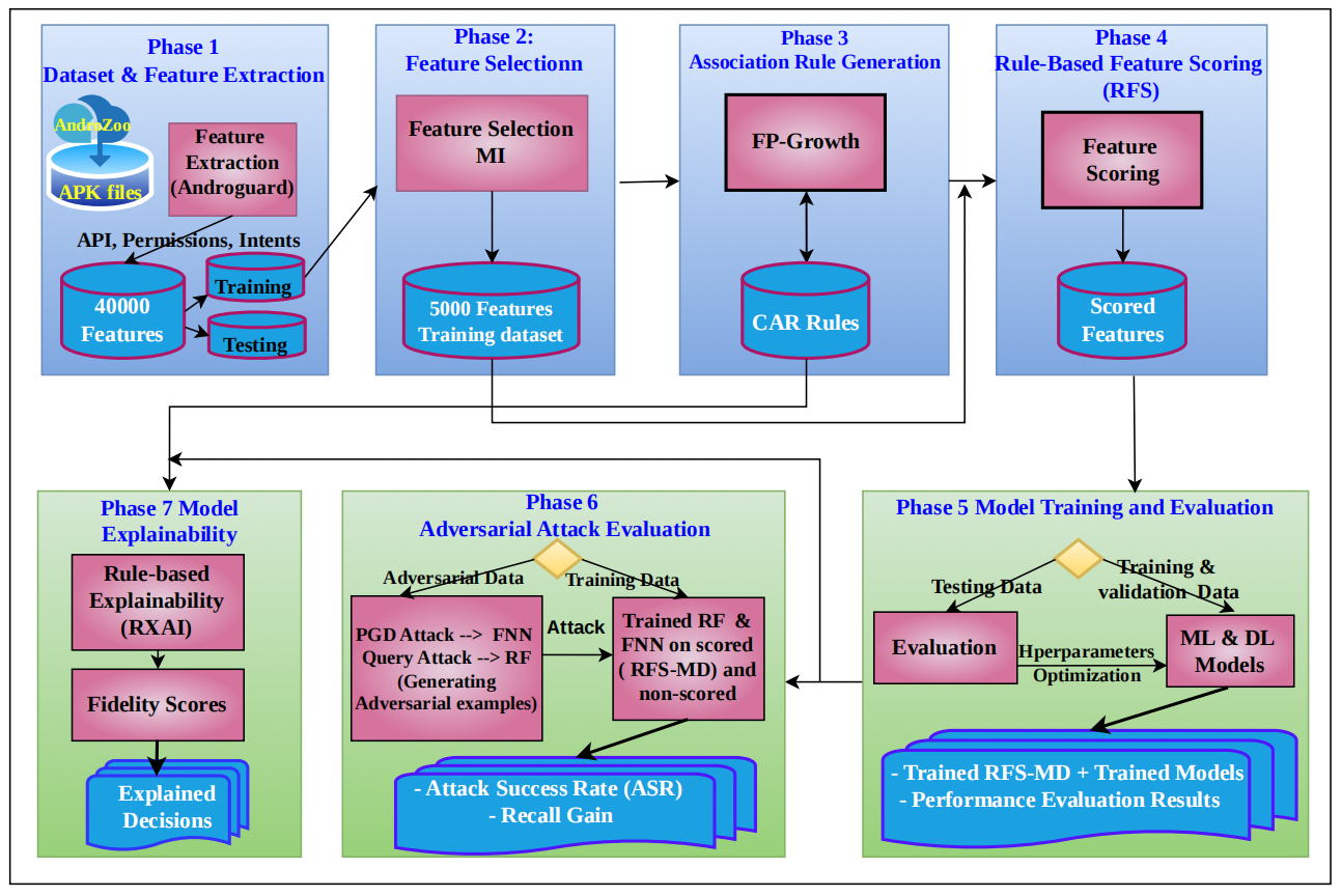
This section presents the methodology of our proposed RFS-MD framework applied in this work regarding ML and DL used under different configurations, adversarial attacks, and explainability. The goal is to develop a comprehensive framework to enhance the performance of explainable malware detection Models and their robustness under adversarial attacks. Starting with extracting the static Android features from APK files. The dataset was divided into a training dataset and a test set, with 85% and 15%, respectively, using a stratified split to preserve class distribution. On the training dataset, we reduced feature dimensionality using the mutual information selection method, preserving highly informative features. Class Association Rules (CARs) are generated using the FP-Growth algorithm. The CARs rules are used in the proposed rule-based feature scoring (RFS) approach to replace binary feature representations with scored feature representations based on rule confidence values. The scored features dataset is used to train several ML and DL classifiers to enhance their malware detection performance and to increase their robustness against adversarial attacks. In addition, CAR’s rules are used to support the explainability of model decisions. To avoid data leakage in model training and evaluation, we performed feature selection, rule generation, and feature scoring exclusively on the training set. Figure 1 illustrates the main procedures of our proposed methodology. The general framework is summarized in Algorithm 1, while the details of each phase are described in the following subsection.

Algorithm 1:Proposed Explainable Malware Detection Framework

Require:  APK samples collected from AndroZoo repository Ensure:  Malware detection models, explainable rules, and adversarial robustness evaluation Phase 1: Dataset Preparation and Feature Extraction 1: $Dataset\leftarrow$ Algorithm 2 Phase 2: Feature Selection using Mutual Information 2: $ReducedDataset\leftarrow$ Algorithm 3 Phase 3: Association Rule Generation using FP-Growth 3: $CAR\leftarrow$ Algorithm 4 Phase 4: Rule-Based Feature Scoring (RFS) 4: $(ScoredDataset,BinaryDataset)\leftarrow$ Algorithm 5 Phase 5: Models Training Including RFS-MD and Evaluation 5: $Models\leftarrow$ Algorithm 6 Phase 6: Adversarial Attack Evaluation 6: $Attacksuccessrate\left(ASR\right),RecallGain\left(RG\right)\leftarrow$ Algorithm 7 Phase 7: Rule-Based Explainability (RXAI) and Fidelity Evaluation 7: $explanations,Fidelity\leftarrow$ Algorithm 8 8: return$Models$, explanations, and adversarial robustness results

3.1. Dataset preparation

The dataset was obtained from the Androzoo repository [35], which is publicly available, contains millions of Android applications from different sources such as play.google.com or appchina, and has been widely used in malware analysis and malware detection research [36]. In addition, it provides many options before downloading the datasets, including the number of VirusTotal (VT) engines used to flag the APK files as malware apps, APK size, APK date, scanning date, the package name, and version code of the APK. We choose to download malware with VT more than 30 times to guarantee that malware samples are strongly flagged as malware. For this study, 9000 Android files were downloaded from the Androzoo database, with 4500 each assigned to malware and benign categories, creating a balanced dataset. We applied the Python Androguard toolkit to parse Android manifest and Dex files to extract static features (API calls, Permissions, and Intents), where we got a high dimensionality of 40000 binary sparse features. Each sample in the dataset is a feature vector, where a value of 1 represents the presence of the feature, and 0 means the absence of the feature. We have two class labels: malware is the positive label with a value of 1, and benign is the negative label with 0 value. This is considered a baseline dataset, which we refer to in this study as a non-scored feature dataset. Dataset preparation and feature extraction are described in Algorithm 2

Algorithm 2:Dataset Preparation and Feature Extraction

Require:  APK samples downloaded from AndroZoo Ensure:  Binary feature dataset 1: $MalwareSamples\leftarrow$ APKs with VirusTotal detection $>30$ 2: $BenignSamples\leftarrow$ APKs with VirusTotal detection $=0$ 3: $n\leftarrow$ total number of APK samples (9000) 4: for$i=1$ to n do 5:     $(Manifes{t}_i,De{x}_i)\leftarrow AnalyzeAPK\left(AP{K}_i\right)$ using Androguard 6:     Extract $API{s}_i$, $Per{m}_i$, $In{t}_i$ from $Manifes{t}_i$ and $De{x}_i$ 7:     for each feature f in $Feature\_Set$ do 8:         if f exists in $AP{K}_i$ then 9:            $FeatureVecto{r}_i\left[f\right]\leftarrow 1$ 10:         else 11:            $FeatureVecto{r}_i\left[f\right]\leftarrow 0$ 12:         end if 13:     end for 14:     if $AP{K}_i\in MalwareSamples$ then 15:         $Labe{l}_i\leftarrow 1$▹ 1 represents malware 16:     else 17:         $Labe{l}_i\leftarrow 0$▹ 0 represents benign 18:     end if 19: end for 20: $Dataset\leftarrow$ combine all $(FeatureVecto{r}_i,Labe{l}_i)$ 21: return Dataset

3.2. Feature Selection and Dimensionality Reduction

The baseline dataset is sparse. We applied the MI algorithm to reduce the dimensionality of the features and select the most informative features that have a high dependency on the class label, keeping the features that contribute more to building a classification model, as shown in Equation (1) [37].

$$MI(X;Y)=\sum _{x\in X}\sum _{y\in Y}p(x,y)log\left({\displaystyle \frac{p(x,y)}{p\left(x\right)p\left(y\right)}}\right)$$

(1)

X symbolizes static features, and Y represents the class label (malware or benign). P(x,y) is the probability that x and y occur together.

The optimal number of features (k) in MI was determined by performing MI score distributions on all 40000 features with the elbow method. As Figure 2 shows, a highly skewed pattern with an inflection point where the MI score drastically decreased after k= 5000. This indicates that a small number of features depend on the class label, while the majority of features are nearly independent or are noise. In addition, another experiment was applied with a minimum MI threshold value of 0.001 to remove all near-zero MI scores, where the feature space was reduced to 5029. Based on these findings, the baseline dataset was reduced to 5000 features. This reduction preserved the most informative features that enhance model performance and decreased model complexity, computational cost, and memory consumption, which is critical for large-scale malware analysis. Features selection process using MI is illustrated in Algorithm 3

Algorithm 3:Feature Selection using Mutual Information

Require:  Binary feature dataset $Dataset$ Ensure:  Reduced feature set $ReducedDataset$, $TestSet$ 1: Split $Dataset$ into TrainingSet and TestSet with 85% and 15%, respectively 2: Compute $MI(f,Label)$ for each feature f in $TrainingSet$ 3: Plot MI scores to generate Elbow Diagram 4: $k\leftarrow 5000$▹ Elbow observed where MI drops sharply 5: Sort $FilteredFeatures$ in descending order based on $MI(f,Label)$ 6: $SelectedFeatures\leftarrow$ top k features from $FilteredFeatures$ ▹$k=5000$ most informative features 7: $ReducedDataset\leftarrow TrainingSet$ restricted to $SelectedFeatures$ 8: return$ReducedDataset$, $TestSet$

3.3. Rules Generation

The overall processing pipeline for rule generation is illustrated in Algorithm 4. First, the Fp-Growth algorithm was applied on the selected features to generate frequent itemsets with a minimum support value (minsup) threshold of 0.01, where each itemset produced includes several related features. FP-growth algorithm discovers the hidden pattern and the relationships between features (items) [38], reducing the cost of searching time and memory consumption compared to other methods of Association Rule Mining (ARM) like the Apriori algorithm, which makes it the best choice to mine the rules for large high-dimensional datasets [39]. Minsup is used to filter out the itemsets with weak frequencies, as shown in Equation (2), where the support of Itemset (A, B) represents the percentage of samples that include features A and B over all samples in the dataset (D).

$$\mathrm{Sup}(A,B)={\displaystyle \frac{|S_{A,B}|}{\left|D\right|}}$$

(2)

Second, is to mine rules, where rules in ARM are mined from each itemset, considering all possible combinations of the items (features) to shape the items of the left-hand side of the rule (antecedent) and the right-hand side of the rules (consequent) [40]. Each mined rule has its own confidence value, which is calculated as shown in Equation (3).

$$\mathrm{Conf}(A\Rightarrow C)={\displaystyle \frac{\mathrm{Sup}(A\cup C)}{\mathrm{Sup}\left(A\right)}}$$

(3)

where A and C could be one feature or a subset of features from the related mined itemset. Confidence values express how strongly the rule is likely to happen [41]. If the confidence of a rule was 80%, when the features in A are present in a specific sample, it is most likely with 80% that features in C are also present in the same sample. Since confidence value is calculated based on item frequencies over the whole dataset, the rule provides global feature relationships, not a feature-sample relationship, and this is another reason for choosing rules generation from ARM.

We only filtered the rules called Classification Association Rule (CAR) [42]. In this type of rule, the consequent is either malware or benign. To produce CAR rules, we add malware and benign features to the dataset with a binary value indicating the presence of these features in the samples. For example, if the sample is malware, in the "malware" feature column, the feature has a value of 1, and the "benign" feature column has a value of 0. So it becomes a part of the itemset when generated by the FP-Growth algorithms. In the CAR Rule, confidence demonstrates how likely the rule is to happen between the samples of malware or benign, reflecting the presence of antecedent rule features within malware samples or benign samples. Only CAR rules are kept in a separate dataset, where they are used in two main phases of our proposed framework. Rule-based scoring phase and explainability phase. The rule generation phase is summarized in Algorithm 4.

Algorithm 4:Association Rule Generation using FP-Growth

Require:  ReducedDataset with selected features Ensure:  Set of Association Class Rules $Rules$ 1: Transform $ReducedDataset$ into transaction format 2: $MinSupport\leftarrow$ predefined minimum support threshold 3: $MinConfidence\leftarrow$ predefined minimum confidence threshold 4: $FrequentItemsets\leftarrow$ FP-Growth mining on FP-Tree 5: for each itemset I in $FrequentItemsets$ do 6:     if I contains class label $\left\{malware\right\}$ or $\left\{benign\right\}$ then 7:         $Antecedent\leftarrow I-ClassLabel$ 8:         $Consequent\leftarrow ClassLabel$ 9:         Compute rule confidence: 10:         if $Conf\ge MinConfidence$ then 11:            $Rules\leftarrow Rules\cup (Antecedent\Rightarrow Consequent)$ 12:         end if 13:     end if 14: end for 15: return$Rules$

3.4. Rule-Based Feature Scoring

For each sample in the dataset, we select the high-confidence CAR rules that match that sample, which means the antecedent features in the selected rules are present in the sample. Only rules with confidence greater than 0.7 are kept to ensure the reliability and statistically meaningful patterns in the scoring process while reducing the noise of weak rules. During scoring, not all rules were used; instead, they were selected based on a priority strategy that supports larger antecedent sizes and higher confidence values. Rules with the same size are stored in descending order of confidence, and only rules with disjoint features are selected to avoid redundancy and ensure feature coverage for the sample. Then the existing features in the sample are assigned the confidence value of the rule that matched those features. We repeated this process to score all features in all samples, producing a new scored feature dataset. This dataset preserves the original features with additional information, which are represented by feature scores that reflect their importance and how much they are related to the class label. The rule consequent (malware or benign) is not used during scoring, which prevents label leakage when producing the scored features dataset.

At the end of this phase, two training datasets are produced: the dataset generated after the feature selection phase, which we refer to as the non-scored features dataset (baseline dataset), with binary features. The scored feature dataset was generated by our proposed rule-based feature scoring (RFS) technique. Both datasets were used to train the ML and DL models under the same experimental conditions and parameters. The rule-based feature scoring technique is illustrated in Algorithm 5.

Algorithm 5:Rule-Based Feature Scoring (RFS)

Require:  Binary feature dataset D, Association Class Rules $CAR$ Ensure:  $ScoredDataset$, $BinaryDataset$ 1: $BinaryDataset\leftarrow D$ 2: for each sample $S_i$ in D do 3:     $SelectedRules\leftarrow \varnothing$ 4:     $UsedFeatures\leftarrow \varnothing$ ▹ Select rules matching the sample 5:     $CA{R}_{candidate}\leftarrow \{r\in CAR\mid antecedent\left(r\right)\subseteq features\left(S_i\right)\}$ 6:     Group $CA{R}_{candidate}$ by rule size 7:     for rule size z from largest to 1 do 8:         Sort rules of size z by confidence in descending order 9:         for each rule r do 10:            if $antecedent\left(r\right)\cap UsedFeatures=\varnothing$ then 11:                $SelectedRules\leftarrow SelectedRules\cup \left\{r\right\}$ 12:                $UsedFeatures\leftarrow UsedFeatures\cup antecedent\left(r\right)$ 13:            end if 14:         end for 15:     end for ▹ Assign feature scores 16:     for each rule r in $SelectedRules$ do 17:         for each feature $f\in antecedent\left(r\right)$ do 18:            $FeatureVecto{r}_i\left[f\right]\leftarrow confidence\left(r\right)$ 19:         end for 20:     end for 21:     Add $FeatureVecto{r}_i$ to $ScoredDataset$ 22: end for 23: return$ScoredDataset$, $BinaryDataset$

The extra computational overhead of the proposed framework compared to the ML malware detection model is confined to an offline preprocessing phase, where the high-confidence rules generation process is performed once on the selected features by the MI algorithm, and the CAR rules are stored for reuse. FP-Growth has high complexity, but its execution depends on the selected features and the minimum support threshold. The rule-based feature scoring (RFS) matches the sample features with the selected CAR rule dataset, where the complexity is proportional to the number of rules and features, but this process is performed only once to produce a scored features dataset to train all ML classifiers. For deployment cases, only the lightweight scoring process is performed on new samples without using FP-Growth or retraining the models. So the proposed framework has a limited cost with maintaining suitability for real-time applications.

3.5. Experimental Setup

This subsection provides the experimental configurations adopted to evaluate the proposed RFS scoring method and evaluate our proposed malware detection method against adversarial attacks. Classification models were evaluated under a scored and a non-scored features dataset for both default and tuned parameter settings. evaluation metrics used to assess the malware detection performance with the same training and testing protocol for all types of models and parameter settings.

3.5.1. Classification Models

To evaluate the effectiveness of our proposed rule-based feature scoring technique (RFS), multiple widely used ML and DL models based on the literature were implemented. DT, KNN, RF, LR, SVM, CNN, and FNN. [43,44] DT is a tree-based classifier covering the feature vectors into tree partitions, presenting decision rules, while RF merges several decision trees for better accuracy and generalization performance. KNN is a distance-based classifier that assigns the new incoming instance the most common label based on the closest k samples. SVM finds the optimal decision boundary that maximizes the margin between classes. In addition to these previous classifiers, two neural network architectures were implemented as deep learning models. CNN was used to find feature patterns using the convolutional and pooling layers, while FNN contains multiple hidden layers to capture the high-level complex nonlinear features and learn to discriminate them for the classification process. This diversity of model types allow to evaluate our approach under several malware detection models, including linear models, distance-based methods, ensemble learners, and deep neural networks.

3.5.2. Evaluation Metrics

The model’s performance was assessed using standard evaluation metrics that include accuracy (Equation 4), precision (Equation 5), recall (Equation 6), and F-score (Equation 7), where they were calculated based on the confusion matrix [45]. These metrics were selected because they are widely applied in malware detection and provide a comprehensive evaluation of classification behavior [28], such as accuracy, which is the percentage of correctly classified samples among all dataset samples. Recall value, which is the most important metric in this study, where it represents the percentage of actual malware that was successfully detected. A higher recall value indicates the system can discover most of the malware and doesn’t miss any. While the precision value expresses how many of the samples classified as malware are truly malware, Low precision indicates that the system has many false alarms

$$Accuracy={\displaystyle \frac{TP+TN}{TP+TN+FP+FN}}$$

(4)

$$Precision={\displaystyle \frac{TP}{TP+FP}}$$

(5)

$$Recall={\displaystyle \frac{TP}{TP+FN}}$$

(6)

$$F_1={\displaystyle \frac{2\times Precision\times Recall}{Precision+Recall}}$$

(7)

Where the true positives $TP$ are the number of malware samples correctly detected, and a high $TP$ means the system is effective in finding threats. While the true negative samples $TN$ represent the number of benign samples correctly identified. High $TN$ reduces unnecessary user alerts. False positives $FP$ indicate benign apps incorrectly classified as malware. Too many $FP$ increases the false alarm, leading to user frustration and loss of trust. In contrast, false negative $FN$ samples are malicious software incorrectly classified as benign. This is the most dangerous error, as undetected malware can compromise security. On the other hand, we used the performance gain to demonstrate the improvement of using our proposed rule-based feature scoring across all models and parameter settings. Performance gain is calculated as the difference between the performance of the scored feature and the performance of the Non-Scored feature, where if the result of the gain was positive, this indicates that using scored features demonstrates improvement [46]. The accuracy Gain (AG) value is calculated as shown in Equation (8), and the recall gain (RG) value is calculated as shown in Equation (9), where S denotes the performance of the scored features and $NS$ represents the performance of the non-scored features.

$$AG=Acc\left(S\right)-ACC\left(NS\right)$$

(8)

$$RG=Rec\left(S\right)-Rec\left(NS\right)$$

(9)

3.5.3. Default Hyperparameters

We trained and evaluated classifiers on their default hyperparameter configurations based on Scikit-learn and TensorFlow librarie. These initial settings provide a baseline for evaluating the ML and DL models’ performance before applying hyperparameter optimization. Table 1 summarizes the default parameter values for all classifiers, which were implemented on both scored and no-scored features datasets to guarantee consistent experimental conditions across all models.

3.5.4. Hyperparameter Optimization

In these evaluation experiments, each classifier was tuned to find the best parameters that yield the best performance. This hyperparameter optimization ensures fairness in the evaluation process and finds the best model’s performance. A grid search strategy with 5 cross-validation was implemented during the tuning process for all classifiers, due to its ability on systematic searching for the best parameters among all possible combinations of available grid values, and identify optimal model configurations. Table 2 summarizes classifiers’ key parameters that were explored during the grid search process to find the best parameters. All sequential procedures of model training and performance evaluation with hyperparameter optimization are demonstrated in Algorithm 6.

Algorithm 6:Model Training and Hyperparameter Optimization

Require:  $BinaryDataset$, $ScoredDataset$, $TestSet$ Ensure:  Trained models and performance evaluation results 1: $Classifiers\leftarrow$ {DecisionTree, KNN, LogisticRegression, RandomForest, SVM, CNN, FNN} 2: for each dataset D in $\{BinaryDataset,ScoredDataset\}$ do 3:     for each classifier C in $Classifiers$ do ▹ Configuration 1: Default Parameters 4:         Initialize C using default parameters 5:         Train C on D 6:         $Predictions\leftarrow C\left(TestSet\right)$ 7:         Compute evaluation metrics (Accuracy, Precision, Recall, F1-score, Accuracy gain, Recall gain) 8:         Store results for C under default configuration ▹ Configuration 2: Tuned Parameters 9:         Define key hyperparameters search space for classifier C 10:         Apply Grid Search with 5-fold cross-validation on D 11:         Test all combinations of hyperparameter values 12:         $C_{best}\leftarrow$ model with best cross-validation performance 13:         Train $C_{best}$ on D 14:         $Predictions\leftarrow C_{best}\left(TestSet\right)$ 15:         Compute evaluation metrics (Accuracy, Precision, Recall, F1-score, Accuracy gain, Recall gain 16:         Store results for tuned configuration 17:     end for 18: end for 19: return performance comparison results

3.6. Adversarial Attack Configuration

To evaluate the robustness of our proposed malware detection models against adversarial applications, a framework for adversarial attacks was designed to simulate realistic adversarial examples. Where the examples are generated by adding benign related features to the malware apps, causing perturbations in their values from 0 to 1. The approach does not enforce semantic dependencies between APK features, and therefore, the generated samples may not always correspond to fully functional APKs. However, these manipulations happened at the feature level, which is widely used in adversarial ML to systematically evaluate model robustness under controlled perturbations rather than a full problem-space attack on executable applications. The adversarial attack used focuses on adding features, not removing them, which aligns with realistic attack behavior, where attackers attempt to fool the detection model into misclassifying malware samples without disrupting its core functionality.

We trained baseline models on the original binary features, and the RFS-MD models were trained on the scored features. This setup ensures identical training configurations and fair comparisons, allowing the evaluation to focus on the intrinsic robustness of the RFS mechanism. Therefore, any improvements in the RFS-MD model against the attack will refer to the enhanced features representation by the RFS technique and the model itself rather than using adversarial examples during training, confirming the robustness of the proposed approach in defending against unseen attacks.

The original dataset of the binary static features extracted from Android applications was divided into two datasets: one with 60% of the dataset to train our proposed RFS-MD model, and the baseline model. To train our RFS-MD model, the dataset must be scored using a rule-based scoring approach before being fed to the model. The other 40% of the dataset is used to generate adversarial examples and evaluate the models under the attacks of these examples. Several adversarial datasets were generated by attacking k features across all samples, where k represents the number of manipulated features. Increasing k will increase the strength level of the attack.

Two classifiers used in adversarial attack experiments, RF and FNN, because they show strong performance gain in recall during malware detection performance experiments. In addition, they belong to different classifier types, where RF is an ensemble learning method based on merging multiple decision trees, while FNN is a deep learning classifier. To generate adversarial examples, a project gradient descent (PGD) attack algorithm was conducted against FNN, because NN is a differentiable classifier, depending on the gradient descent algorithm to optimize the classification performance, PGD is a white-box attack that computes gradients to modify effective features and generate adversarial examples [47]. While RF is non-differentiable, a gradient-based attack cannot be implemented directly. We used a query-based greedy feature attack as a black-box attack, where it iteratively flips feature values from 0 to 1 while querying the model for the minimum predicted malware probability [48]. Applying this attack strategy allows us to evaluate how our proposed RFS-MD model enhances resistance under gradient-based attacks and query-based attacks.

We evaluate the model’s resistance against the adversarial attack, using recall gain and attack success rate (ASR). The ASR is the percentage of malware samples that successfully evade model detection after attacking their features [43], where it measures the effectiveness of adversarial attacks. as shown in Equation (10), where $N_{success}$ denotes the number of successful adversarial examples and $N_{attack}$ is the total number of all malware samples.

$$ASR={\displaystyle \frac{N_{success}}{N_{attackk}}}\times 100$$

(10)

While recall gain measures the improvement in resistance of our proposed model, RFS-MD, compared with the baseline model’s resistance. Adversarial Attacks methodology, including attack algorithms and evaluation metrics, is described in Algorithm 7.

Algorithm 7:Adversarial Attack Evaluation using Feature based attack

Require:  D (original binary feature dataset), $k\_list$ (attack budgets), $classifiers=\{RF,FNN\}$, $scoring\_rules$ Ensure:  Evaluation metrics for each attack budget 1: Split dataset D 2: $TrainSet\leftarrow 60\%$ of D 3: $AttackSet\leftarrow 40\%$ of D ▹ Apply rule-based feature scoring 4: $Train\_scored\leftarrow scoring\left(TrainSet\right)$ ▹ Train RF and FNN on TrainSet and Train_scored 5: $R{F}_{scored}\leftarrow train(RF,Train\_scored)$ 6: $R{F}_{baseline}\leftarrow train(RF,TrainSet)$ 7: $FN{N}_{scored}\leftarrow train(FNN,Train\_scored)$ 8: $FN{N}_{baseline}\leftarrow train(FNN,TrainSet)$ 9: for each classifier C in $\{RF,FNN\}$ do 10:     for each attack budget k in $k\_list$ do 11:         for each malware sample x in $AttackSet$ do 12:            if $C=RF$ then 13:                $x_{adv}\leftarrow GreedyBlackBoxAttack(x,k)$ 14:            end if 15:            if $C=FNN$ then 16:                $x_{adv}\leftarrow PGD\_Attack(x,k)$ 17:            end if 18:         end for 19:         $D_k^{adv}\leftarrow$ adversarial dataset generated with budget k ▹ Apply rule-based scoring on adversarial samples 20:         $D_{scored}^{adv}\leftarrow scoring\left(D_k^{adv}\right)$ ▹ Evaluate models 21:         $R{F}_{scored\_results}\leftarrow evaluate(R{F}_{scored},D_{scored}^{adv})$ 22:         $R{F}_{baseline\_results}\leftarrow evaluate(R{F}_{baseline},D_k^{adv})$ 23:         $FN{N}_{scored\_results}\leftarrow evaluate(FN{N}_{scored},D_{scored}^{adv})$ 24:         $FN{N}_{baseline\_results}\leftarrow evaluate(FN{N}_{baseline},D_k^{adv})$ ▹ Compute evaluation metrics 25:         Compute Attack Success Rate (ASR) 26:         Compute Recall Gain 27:         Store results for attack budget k 28:     end for 29: end for 30: return evaluation results

3.7. Explainability Analysis

To enhance the explainability of the proposed malware detection model, we introduce a Rule-based Explainable Artificial Intelligence (RXAI) approach. In this phase, we use the Class Association Rules (CARs) dataset generated in Algorithm 4 to provide human-understandable explanations for each prediction. The proposed RXAI approach works as a post-hoc agnostic model with Local and global explanations, focusing on rule-based explanations.

3.7.1. Rule-Based Explanations

To provide model decision explanations to our proposed model RFS-MD, for each sample $S_i$, we identified the set of rules from the CARs dataset whose antecedent features are present in the relevant sample. The top K rules are selected based on the highest confidence values, starting from the largest size without any overlap with the features associated with the top K selected rules, following the same strategy that we used to select the rules for the scoring process. Then the selected rules are used to provide human-understandable explanations for model classification decisions by showing the most influential interacting features that contribute to the model’s decision and how confident they are associated with the class label, providing transparent and explained decisions.

3.7.2. Fidelity Evaluation of Rule-Based Explanations

To evaluate the proposed RXAI model quantitatively, we proposed a fidelity approach to evaluate the effectiveness of model decision explanations. The fidelity metrics measure how much change in the model prediction values per sample occurs before and after removing the features involved in the top rules, evaluating the level of explainability of the top rules of the model. Higher fidelity means that the rules that are used to explain model decisions for the sample $S_i$ include the most critical interacting features and relations that contributed to the class label, which lead to transparent and reliable explanations. As Equation (11) shown, the fidelity score is computed for each sample by the absolute value of the difference between the original prediction probability $P_{\mathrm{original}}$ and the modified prediction probability $P_{\mathrm{modified}}$ after removing the features of the model’s top k explaining rules [49].

$$\mathrm{Fidelity}=\left|P_{\mathrm{original}}-P_{\mathrm{modified}}\right|$$

(11)

The fidelity calculated at the sample level considers local fidelity. While the observed distributions and statistical measures (mean and median) provide an aggregated view of global fidelity, which reflects how well the extracted rule set collectively represents the overall behavior of the model across multiple samples. The proposed RXAI approach, including explaining rules and fidelity evaluation, is described in Algorithm 8.

Algorithm 8:Rule-based Explainability RXAI and Fidelity Evaluation

Require:  Binary feature dataset D, Association Class Rules CAR, Trained model M, Number of rules k Ensure:  Explanations and fidelity scores for each sample 1: for each sample $S_i$ in D do 2:     $SelectedRules\leftarrow \varnothing$ 3:     $UsedFeatures\leftarrow \varnothing$ ▹ Select rules matching the sample 4:     $CA{R}_{candidate}\leftarrow \{r\in CAR\mid antecedent\left(r\right)\subseteq features\left(S_i\right)\}$ 5:     Group $CA{R}_{candidate}$ by rule size 6:     for rule size z from largest to 1 do 7:         Sort rules of size z by confidence in descending order 8:         for each rule r do 9:            if $antecedent\left(r\right)\cap UsedFeatures=\varnothing$ then 10:                $SelectedRules\leftarrow SelectedRules\cup \left\{r\right\}$ 11:                $UsedFeatures\leftarrow UsedFeatures\cup antecedent\left(r\right)$ 12:            end if 13:         end for 14:     end for 15:     Extract contributing features: $$F_i=\bigcup antecedent\left(r\right),r\in \mathrm{Top}-k\mathrm{rules}$$ 16:     Compute original prediction: $$P_{\mathrm{original}}=M\left(S_i\right)$$ 17:     Remove features $F_i$ from $S_i$ to obtain modified sample $S_i^{\prime }$ 18:     Compute modified prediction: $$P_{\mathrm{modified}}=M\left(S_i^{\prime }\right)$$ 19:     Compute fidelity: $$Fidelit{y}_i=|P_{\mathrm{original}}-P_{\mathrm{modified}}|$$ 20:     Generate explanation using selected rules and their confidence 21: end for 22: return Explanations and Fidelity Scores

4. Experimental results

This section presents the experiments performed and the results obtained through this research on three main types of experiments, alongside the results analysis. First, the findings of the experiments obtained by evaluating classifiers of ML and DL on both scored and non-scored feature datasets, under both default and tuned parameters. Second, adversarial attack experiments to evaluate model robustness. Third, model decision explanations.

4.1. Impact of Rule-based Feature Scoring on Malware Detection

4.1.1. Performance with Default Parameters

In this type of experiment, all ML and DL models are conducted on both datasets (scored and non-scored) using the default hyperparameter setting based on Scikit-learn and TensorFlow libraries with their standard configurations, as shown in Table 1. The results show that our proposed RFS scoring technique improves the model’s malware detection performance across all classifiers, where the accuracy and F-Score values for all classifiers on the scored datasets are higher than their values on the non-scored dataset. Figure 3 shows the accuracy behavior across all classifiers on both datasets. Random Forest achieved the highest accuracy on the scored dataset with 98.584%, followed closely by Logistic Regression with 98.510%. The non-scored dataset, RF classifier achieved an accuracy of 98.212%, which is also the highest accuracy across all classifiers. This indicates that even for very effective ensemble models, RFS scoring affords tangible improvements. For the classical ML classifiers, the scored features dataset outperformed the non-scored dataset. DT accuracy and F-score increased from 95.157% to 95.827% and from 95.217% to 95.876%, respectively, while KNN accuracy increased from 94.784% to 95.753%. LR has more improvements using scored features, where the accuracy increased from 97.243% to 98.510%, reflecting the strong effectiveness of the linear decision boundaries. SVM has a few improvements, where accuracy increased from 97.616% to 97.839%. For the deep learning model, CNN achieved 97.839 on the scored dataset compared to 97.765% on the non-scored dataset. FNN’s performance also increased, rising from 97.168% to 97.616% when trained on the scored features.

Table 3. Classification performance using default parameters on scored and non-scored feature datasets.

Classifier	Dataset	Acc (%)	Prec (%)	Rec (%)	F-Score (%)
DT	Scored Features	95.827	95.315	96.444	95.876
	Non-Scored Features	95.157	94.591	95.852	95.217
KNN	Scored Features	95.753	98.892	92.593	95.639
	Non-Scored Features	94.784	98.400	91.111	94.615
LR	Scored Features	98.510	98.375	98.667	98.521
	Non-Scored Features	97.243	97.612	96.889	97.249
RF	Scored Features	98.584	98.378	98.815	98.596
	Non-Scored Features	98.212	98.655	97.778	98.214
SVM	Scored Features	97.839	98.353	97.333	97.841
	Non-Scored Features	97.616	98.638	96.593	97.605
CNN	Scored Features	97.839	96.812	98.963	97.876
	Non-Scored Features	97.765	97.496	98.074	97.784
FNN	Scored Features	97.616	97.210	98.074	97.640
	Non-Scored Features	97.168	98.185	96.148	97.156

Table 3. Classification performance using default parameters on scored and non-scored feature datasets.

Classifier	Dataset	Acc (%)	Prec (%)	Rec (%)	F-Score (%)
DT	Scored Features	95.827	95.315	96.444	95.876
	Non-Scored Features	95.157	94.591	95.852	95.217
KNN	Scored Features	95.753	98.892	92.593	95.639
	Non-Scored Features	94.784	98.400	91.111	94.615
LR	Scored Features	98.510	98.375	98.667	98.521
	Non-Scored Features	97.243	97.612	96.889	97.249
RF	Scored Features	98.584	98.378	98.815	98.596
	Non-Scored Features	98.212	98.655	97.778	98.214
SVM	Scored Features	97.839	98.353	97.333	97.841
	Non-Scored Features	97.616	98.638	96.593	97.605
CNN	Scored Features	97.839	96.812	98.963	97.876
	Non-Scored Features	97.765	97.496	98.074	97.784
FNN	Scored Features	97.616	97.210	98.074	97.640
	Non-Scored Features	97.168	98.185	96.148	97.156

In malware detection, precision and recall are informative for the reliability and sensitivity of malware detection. In this study, since we consider the malware as the positive label with 1, recall here represents the percentage of the actual malware that was detected successfully. A higher recall value indicates the system can discover all malware and doesn’t miss any. The precision value expresses how many of the samples classified as malware are truly malware. Low precision indicates that the system has many false alarms.

As Figure 4 (a) shows, DT obtains a precision value of 95.315% and a recall of 96.444% on the scored features, where both are higher than the same values on non-scored features. This indicates that DT benefits from the scored feature technique, where it enhances the ability to detect true malware and lowers the number of false alarms. KNN classifier, as represented in Figure 4 (b), has a higher precision value (98.892%) than recall(92.593%) on the scored dataset, indicating that KNN can predict malware with few false alarms but with missing a subset of malware apps. The same behavior on the non-scored value with slightly lower precision and recall, demonstrating that the scoring approach preserves the same predicting behavior for the KNN classifier, while improving its performance and ability.

LR obtains a high-balanced precision and recall of 98.375% and 98.667%, respectively, on the scored dataset, resulting in discovering nearly all of the malware apps with a few false alarms. As illustrated in Figure 4 (c), on the non-scored features, LR has a lower precision and recall value with 97.612% and 96.889%. This demonstrates that a rule-based feature scoring approach significantly enhances LR. RF shows high precision and recall on both datasets, where on the scored features it has a precision of 98.378% and a higher recall of 98.815% as presented in Figure 4 (d). This indicates that RF with scored features has a very efficient detection ability, where it nearly doesn’t miss any malware and has almost zero false positives. On the other hand, precision is slightly higher with 98.655% on the non-scored dataset, but recall decreases to 97.778%. The scored dataset enhances recall and overall f-score (98.596%), confirming it has balanced detection behavior and strong reliability.

SVM achieves a precision of 98.353% and a recall of 97.333%. Precision is higher than recall, indicating that it has lower false alarms but misses a subset of malware samples. On the non-scored features, precision increases to 98.638%, while recall decreases to 96.593%. As shown in Figure 4 (e), the scored features enhance recall and reduce precision a little bit, but overall result in a higher F-score (97.841%). This indicates that feature scoring supports SVM to detect more malware samples without noticeably worsening the number of false alarms. CNN obtains a precision of 96.812% and the highest recall value with 98.963% in all classifiers using the scored. CNN almost doesn’t miss any malware, but can produce some false alarms. As Figure 4 (f) illustrates, the non-scored features increase precision and reduce recall, demonstrating that the scored dataset improves the classifier’s malware detection sensitivity. On the other hand, FNN has a precision value of 97.21% and a higher recall value of 98.074% for the scored features. While it obtains higher precision (98.185%) and lower recall (96.148%). As Figure 4 (g) shows, the scored features significantly improve the recal, resulting in a higher f-score (97.640%).

Overall, these findings across all classifiers under the default parameters show that our rule-based feature scoring technique improves malware detection performance, increasing recall and reducing false negatives. The overall balance between precision and recall improves, as shown by higher F-scores. These findings confirm that rule-based feature scoring enhances class separability and contributes to more reliable malware detection performance.

The gain values in accuracy and recall for all classifiers are shown in the chart in Figure 5 and clearly show the overall benefit of using the rule-based features scoring over the original non-scored features. The accuracy improvements show that three classifiers (DT, KNN, and LR) gained over +0.5%, and KNN and LR have the highest gains, which confirms that distance-based classifiers and linear classifiers have a positive response to the scored features. The highest gain in our research is the recall gain, which indicates how much more efficient the classifier is at finding more samples of malware and not missing any (reducing false negatives, which are the most dangerous because undetected malware can compromise security). The chart shows that all classifiers have gained over 1% in recall, with FNN having the largest improvement at 1.93%, and RF, LR, and KNN also showing above +1%, whereas CNN and SVM have an improvement above 0.5% in recall gain. The improvement in recall gain values across all classifiers (except DT) is greater than the accuracy.

4.1.2. Performance After Hyperparameter Optimization

To ensure the quality, efficacy, and reproducibility of the rule-based feature scoring method, hyperparameter optimization was implemented across all classifiers, tuning the most effective parameters with a wide range of possible values, as shown in Table 2. Table 4 demonstrates the best parameter values for each classifier, while the models’ performance under the tuned configurations is illustrated in Table 5.

The results demonstrate that there is consistent effectiveness of the rule-based feature scoring even under the tuned models. Across all classifiers and optimal model configurations, scored features achieve higher accuracy, recall, and f-score compared with non-scored features, as shown in Figure 6, and achieve higher precision values as well in most classifiers. Our proposed RFS-MD enhances the feature discrimination.

On scored features, LR, RF, SVM, and FNN have accuracy above 98%. While in default parameter settings, only LR and RF have accuracy above 98%. This indicates that model tuning increases accuracy in some models, but the performance behavior remains the same, even with model hyperoptimization on scored and non-scored features. For recall values, it is noticeable that scored features help all models discover the malware sample more effectively, which is a high demand in security applications. In addition, precision values remain high in traditional ML, while it increases in DL models such as CNN and FNN, indicating that the RFS scoring technique doesn’t increase the number of false alarms.

The chart in Figure 7 shows the gain values of the accuracy and recall across all classifiers. similar to the gain behavior of the model under default parameters. The gain results on the tuned models highlight that the classifier’s performance on scored features outperforms the model’s performance on the original dataset. This confirms that our proposed RFS technique enhances feature space representation independently of hyperparameter optimization.

Overall, hyperparameter optimization reinforces the findings obtained from model evaluation under the default parameter experiments. Our RFS scoring method consistently improves malware detection performance across all classifiers, including tree models, distance-based models, linear models, and deep learning models. Scored features have a strong importance score that helps the security model reveal the malware and benign samples’ behavior in a sufficient way.

4.2. Adversarial Robustness Evaluation

In this subsection, we evaluate the robustness of our proposed RFS-MD model and the baseline model on both RF and FNN, reporting ASR values and recall gain for different feature budgets, with K features attacked by the PGD algorithm for FNN and by query-based attack for RF models. Models in these experiments were trained using standard training without adversarial training to ensure that the effectiveness of model robustness is solely attributed to the proposed RFS feature representation.

4.2.1. Adversarial Attack Evaluation on the Neural Network Model

The ASR performance results for scored and non-scored features with the FNN model are depicted in Figure 8. It can be seen that ASR increases with the number of attacks and that for the baseline model trained on binary original features, the ASR starts at 5% when only one feature is attacked for each sample and increases as the number of attacked features increases. When modified features reach 50, the ASR value is higher than 20%, and the attack becomes more effective as the perturbation budgets increase. This trend continues with large feature modifications, with about 52% when 125 features were altered. On the other hand, FNN trained with scored features exhibits much greater robustness to the most powerful adversarial examples, such as ASR falling to 2.3% when $k=1$ (over 50% improvement in our model) and continuously outperforms the baseline model as the perturbation budget increases. ASR with scored features is roughly 34.5% with $k=100$ compared to 45.4% for the baseline model.

For further evaluation, we computed the recall gain for both tested models, where the recall is very important to show how much improvement has occurred in classifying adversarial examples as malware, not benign. The bars in Figure 9 shows that when few features are attacked ($k:1-10$), the recall gain ranges from 2.5% to 3%, indicating that our RFS-MD improves adversarial attack resistance even with small feature perturbations. In addition, we noticed that the recall gain increases as the number of features increases linearly. For example, when $k=10$, the recall gain is approximately 4%, and when $k=30$, it is approximately 6%. This demonstrates that our proposed model not only has a higher recall than the baseline model, but also shows stronger resistance against adversarial attack along a large number of attacked features. Even though the recall gain has a slight fluctuation in more attacks of features, it is still consistently positive at all values of k. The maximum improvement is observed when 115 features were manipulated, where the recall gain reached about 12.5%.

Overall, the RFS-MD model-based FNN classifier reduces ASR values across all perturbation budgets and increases recall gain as manipulated features increase, outperforming the baseline FNN classifier, especially over stronger attacks.

4.2.2. Adversarial Attack Evaluation on the Random Forest Model

Our proposed RFS-MD model-based RF classifier is evaluated by ASR and the recall gain against the baseline RF model that was trained on the original binary features. Figure 10 demonstrates that ASR increases as the number of the attacked features increases at a small level of manipulations for non-scored features, starting from 2.5% at $k=1$, reaching the peak point around $k=17$ with ASR of approximately 6.3% for the baseline RF model. This indicates that adversarial attacks can change the decision paths in RF decision trees. A similar pattern is observed for scored features, where ASR is lower than the baseline at all adversarial attack levels, where the ASR reaches about 5.7% at its peak point with $k=15$, indicating that RFS-MD has a lower peak value that holds maximum ASR, which is also lower than the baseline model.

After the peak point for each model, ASR begins to decrease gradually until reaching 0 value at $k=47$. This trend indicates that for a black-box attack on RF, the number of adversarial malware beyond a certain threshold does not improve its resistance performance. Overall, ASR increases linearly with a small number of perturbations, then gradually declines to zero as k increases.

The recall gain of the RF model is relatively small, but it remains positive across the most adversarial attack levels, as illustrated in Figure 11. The recall gain is improved from 0 at $k=1$ to approximately 1.55% as the highest gain at $k=31$. This demonstrates that the RFS-MD-based RF classifier slightly enhances the adversarial attack detections.

Our RFS-MD model effectively reduces ASR compared to the baseline model that was trained on the original non-scored features across both classifiers, RF and FNN, while maintaining a positive recall gain, confirming its efficacy in enhancing detection system resistance against adversarial malware apps.

4.3. Model Explainability

4.3.1. Rule-Based Explanations of model predictions

To provide human-readable explanations and enhance the explainability of the model’s decisions, we used the same ACR rules dataset obtained during the rule generation phase of our methodology, which includes the rules that capture the relationships between the features and the class, and the interactions among the features that contribute to the model’s decision. In Table 6, we present some of the model decision explanations for some examples of malware and benign samples, along with their top-5 extracted rules that explain model classification decisions. Each rule includes interacting features in the rule antecedent column, its confidence value reflecting its strength, and its label.

In malware samples, the extracted rules consist of informative interacting features relevant to malicious behavior. We will use Sample 998 from the table as a case study to show how to make things clear for the user. Sample 998 has a 0.95% chance of being malware, where the top rules we got show that there is a privacy threat to sensitive data and strange network communication behavior. For example, the features $getLine1Number$ and $getSimSerialNumber$ suggest that the app is trying to get unique device identifiers that can be used to track or profile the user. The rule also includes $getSystemService$ with $android.permission.INTERNET$ means that there may be network communication, which could send data back to servers outside the network. Other rules, like setIcon and setRepeatCount, tell background or repetitive tasks to hide bad behavior by pretending to be normal. In general, the combination of the privacy data access and transmission operations explains why this sample was classified as malware, where these behaviors are strongly associated with data collection and potential exfiltration techniques.

In sample 1815, the highest confidence rules indicate that several malicious tasks are identified through their features, where these tasks could be data exfiltration, network monitoring, device fingerprinting, and propagation via shortcuts. The first rule indicates that the presence of $api\_call\_execSQL$ with the collection of information API using $api\_call\_getExtraInfo$ supports malware behavior, especially since it has a confidence level of 1. The second rule clarifies that monitoring the changes in WIFI state and holding the permission to access WIFI $(ACCESS\_WIFI\_STATE)$ simultaneously indicates network activity tracking, while $onDestroy$ suggests hiding tracking or completing the malicious task before destroying it. In addition, malware can cause installing $SHORTCUT$ combined with internet access and reading the phone state, as the third rule demonstrated. while $getParams$ and $getDeviceId$ APIs are coming together in the fourth rule, indicating for collecting device parameters and IDs. Rule 5 indicates a possible intent of the hijacking process through the custom $addDataScheme$.

According to the extracted rules of sample 275, it attempts to reveal private information and sensitive data from the device while hiding its malicious activities behind normal app operations, where the confidence value of 1 for rules 1 and 2 indicates the semantic strength of these combined features, supporting the idea of applying these operations to hide the malicious main tasks, like animations, rotations, and touch handling. $getSubscriberId$ and $READ\_PHONE\_STATE$ APIs suggest that the app could track data and access sensitive device identifiers, while $api\_call\_writeByte$ and $api\_call\_setWebViewClient$ demonstrate data processing and possible web communication. Overall, these malware rules indicate that the application uses obfuscation techniques and privacy data collection, which explains why the detection model classifies it as malware.

Table 7 shows the rules that explain the model’s decision regarding the two benign samples. Sample 8595 shows normal features related to network requests and caching ($addRequestHeader$, $setAppCachePath$). Rule 2 indicates accessing a file from external storage, while Rule 3 handles downloaded content. It uses cookies and UI, which are normal in regular apps like browsers or content viewers. All these rules reflect the legitimate behaviors for this sample without abnormal actions on sensitive data or hidden activity. In sample 7773, rules related to application settings and user interface actions, without any clear malicious features, were combined with these features. This results in being more benign than malware. APIs here for handling navigation ($canGoBack$, $requestFocus$), touch events, saving preferences, ads display, and screen layout. All these operations are standard for users when interacting with the app, and no high-confidence malware rules exist that carry malicious combined features.

The result shows that the benign classification is not supported only by the presence of benign rules with legitimate semantics, but also by the absence of malicious behaviors, such as combined suspicious APIs and permissions. The first sample has a high prediction value of 0.98, indicating that there is a strong alignment between the model decisions and the high confidence of the top benign rules. The second sample has a lower benign prediction percentage (0.59), considering it as benign. Although its top rules indicate legitimate behavior, they have less distinct benign features and may overlap with features that exist in malware, where confidence decreases significantly starting from the top base, with large differences. These model prediction scores with explanations based on the top rules present a high level of explainability with strength evaluation of the model’s malware detection decisions.

4.3.2. Fidelity Evaluation of Rule-Based Explanations

To evaluate the effectiveness of the decision explanations of our proposed RXAI model, we implemented the fidelity analysis for a large subset of 200 samples (100 malware, 100 benign). The distribution of fidelity scores is shown in the violin plot Figure 12, which provides a comparison between fidelity score distributions for both malware and benign classes. Table 8 presents the Fidelity statistics for malware and benign samples.

For the malware sample, we have wide distributions for fidelity score, which mean for a specific fidelity value, we have a density of malware samples. The mean value is 0.133, with a median of 0.12 and a standard deviation of 0.096. Scores ranging from 0 to 0.52 with density area, indicating that most of the malware samples have observed changes in prediction values. In addition, almost half of the malware samples extend towards higher scores, making a longer upper tail. This violin shape demonstrates the influence of the top rules across different samples in the model explainability process. In contrast, the benign samples have lower fidelity scores and a small density area that is located in the low fidelity values. This indicates that a small number of benign samples have a fidelity of more than 0, with a mean of 0.0185. Samples with the highest scores are rare, with scores up to 0.33. The overall median is 0.01, and the standard deviation is 0.045.

The difference in mean fidelity scores between malware (0.133) and benign (0.0185) indicates the different influence of removing the features of the sample top rules on the two classes, where the shape of the fidelity score distribution and the spread confirm this distinction. From a global perspective, the extracted rules collectively capture the model behavior more effectively for malware samples than for benign samples.

5. Discussion

5.1. Malware Detection Performance

The results of the malware detection model demonstrate that using rule-based feature scoring enhances malware detection performance across all classifiers with both classical ML and DL models. These improvements in all classifiers’ performance are model-agnostic, indicating to enhance the quality of feature representation. The key point is that malware detection performance was enhanced across all classifiers under both default and tuned hyperparameter settings. This indicates that the improvements are not simply a result of model configuration but refer to the rule-based feature scoring efficiency, which operates independently of model-specific optimization, improving the quality and informativeness of the input features themselves.

The most important enhancement is the recall performance across all classifiers, which was obvious in the recall gain for all experiments that cover default and tuned models’ parameters, confirming that our RFS approach is particularly effective in reducing the risk of false negatives, which is a high-demand security where undetected malware can lead to a weakness in the security systems. The ability of the RFS approach to improve the recall without worsening the precision values indicates that it successfully highlights malicious features that have a strong association with the malware class label.

Additionally, the effectiveness of the proposed approach RFS -MD varies across classifier types, where the traditional ML models, such as Decision Trees, KNN, and Logistic Regression, show more enhancement with RFS scoring compared with DL models, demonstrating that traditional ML models depend strongly and explicitly on the feature importance scores unlike DL models, such as CNN and FNN which inherently feature representations. Nevertheless, the consistent improvements resulting in DL models’ performance when using the RFS-DM approach confirm that the rule-based feature scoring mechanism provides complementary information rather than replacing learned representations. The improvement achieved in RF demonstrates that the use of the RFS technique provides global feature importance scores that cannot be captured by local splitting criteria.

The steady improvements across all model types and configurations demonstrate the resilience and robustness of the proposed approach. Our RFS-MD captures interactions between features and their relationships with class labels, and highlights the impact of integrating the association rules into the feature representation space. Table 9 presents a comparison between our proposed RFS-MD approach and some previous related studies. The RFS-MD approach shows a unique and comprehensive approach, maintaining a clear advantage in explainability and robustness. Previous studies [46,50] have enhanced feature representations based on graph learning or multimodal fusion, obtaining high accuracy and recall through the use of complex models. While other studies implemented hybrid feature extraction and ensemble or deep learning models to improve classification results over multiple Android datasets [51,52]. These methods show that they can make good predictions, but depend on either expensive models or complex feature selection and scoring methods. They don’t focus on making the results understandable or maintaining high performance gains across different classifiers.

In contrast, our proposed RFS-MD approach follows a different approach by putting rule-based feature scoring directly into the input feature representation. It uses association rules to highlight the interacting features and their relationships with the class label, adding feature scores and making the feature space expressive and understandable. Unlike traditional feature selection methods, such as Wei et al. and Pathak et al. [53,54], which focus on reducing dimensionality or weighting features based on statistical importance. RFS-MD has the same or better accuracy, up to 98.584%, and always improves the recall in all classifiers, with the best case being 98.815%. Improvements in recall are very important, where many studies either don’t report recall directly or get high accuracy without making sure they can find malware samples. In addition, studies such as [55,56] employ multimodel fusion or redundancy reduction to enhance model performance without improving the recall values or increasing model resistance against adversarial samples.

Overall, the comparisons indicate that other studies work on enhancing malware detection performance or designing feature engineering techniques. While our RFS-MD approach presents more balance and an effective strategy, integrating rule-based feature scoring into the feature representation and uses the extracted rules to provide more explainable decisions. The RFS-MD approach bridges the gaps between performance, robustness, and explainability within a unified framework, addressing important limitations in current malware detection frameworks and providing a deployable and reliable adversarial malware detection system.

5.2. Model Robustness: Adversarial attacks

The results of adversarial attacks implemented show strong evidence that the rule-based features scoring technique effectively enhances the robustness of the malware detection models under both white-box and black-box feature attacks. The consistent trend across all experiments shows that models trained on scored features exhibit lower sensitivity against adversarial perturbations and preserve a higher malware detection performance compared to the baseline model trained on the same non-scored features. This is shown by ASR values results of the implemented models and by the recall gain, which presents the increase in the RFS-MD model recall values over the baseline model recall values on the same number of attacked features.

In the white-box attack, a PGD attack was applied on FNN models, where the ASR values increased sharply as the number of attacked features increased, reflecting the expected behavior of the PGD attacks. However, the degradations in the performance of the model trained on scored features are less severe than the decline in the performance of the model trained on non-scored features, where it has higher ASR values. This is because the rule-based feature scoring technique scores informative features based on high-confidence extracted matching rules, which prioritizes the effective features that are strongly associated with discriminative behaviors of a specific class. As a result, the implemented feature-based attack on less important features has less influence on model decisions, even when it attacks the strongest correlated features; their stronger associations with class make it difficult for the PGD attack to change model decisions.

The positive results of the recall gain of the proposed RFS-MD model indicate that it can correctly identify malware samples even when the number of attacked features increases. This is particularly important in the cybersecurity field, where false negatives lead to a critical risk. In general, the results of recall gain demonstrate that RFS-MD not only enhances classification performance but also improves adversarial attack robustness of malware detection models, making the model more reliable in real-world malware detection scenarios.

In a black-box attack, the robustness of the RF is significantly improved, unlike FNN, which depends on gradients, because the RF uses discrete decision boundaries with the ensemble method, which makes it more resistant against small feature modifications. RF based on the RFS-MD model enhances robustness over a wide range of attack strength levels with little impact on recall. This higher performance of the RF model is due to the combination of the most important interacting features with ensemble decision-making, where the critical features control the splitting points of the decision trees, making it challenging for adversarial feature manipulation to change multiple decision paths simultaneously. In a black-box attack, where attackers do not know the model structure, this impact is further enlarged, and the effectiveness of the attack is reduced.

The findings demonstrate that using the RFS technique improves malware detection performance and increases robustness against adversarial attacks, where the feature importance scores derived from the relevant rules are integrated into the learning process. This makes the model an effective defense mechanism against different types of adversarial attacks in cybersecurity systems.

To further analyze the robustness limits of the proposed framework, we consider a stronger threat model involving an adaptive attacker. The rule dataset, which is used for the feature scoring process, is maintained as a separate and protected component of the deployed trained model. This separation limits direct access to the rule base, reducing the feasibility of white-box attacks. In addition, some security mechanisms could be adopted, such as access control, model–rule decoupling, and secure storage of the rule. Even with partial knowledge of the scoring mechanism, generating adversarial examples remains challenging due to the nature of feature interactions and the multiple rules of high relational features. As a result, the adaptive attacker could attempt to avoid the strongest features, but the structural constraints imposed by the rules inherently increase the difficulty of effective evasion.

5.3. Explainability

Our rule-based explanation method for the malware detection model relies on the relationships among the strongest features of the rules and identifies how much these interacting features push the model to make a decision for one of the class labels. Choosing the top confident rules makes model decisions more understandable by helping malware analysts or security users understand which features could lead to more malicious behaviors, construct a clear idea about complex attack behavior, and identify the malware security-based target. Unlike methods that depend only on important features, which consider isolated indicators in model decisions, making it hard to capture the big picture of the malware target. Consequently, the decision explanations produced by RXAI, as we saw in the explanation results of the malware and benign predicted samples, go beyond conventional feature interpretability. The combinations of features associated with the classification output enable the model to provide actionable insights that can help security analysts understand, verify, and interact with detected threats. In addition to these advantages, it also reinforces trust between users and the security system, especially in cybersecurity fields, where model decisions are no longer treated as a black box, but as logical conclusions derived from informative patterns. As a result, the RXAI approach not only works as an explainability model but also works as a bridge between automated malware detection and security analysis from a human perspective.

The fidelity results show that the proposed RXAI is aligned with the behavior of the model decisions, particularly for malware samples. This indicates that the results’ explanations are not only approximate or heuristic but also refer to the designed prediction model. This alignment is necessary to ensure the reliability and validation of the model’s explainability and provide actionable insight, especially in cybersecurity applications. On the other hand, when we have high fidelity results for the malware samples, it means that the top selected explanation rules carry malicious feature relationships that associate the rule’s features together, at the same time, associate these interactive features with the class label. The large number of malware samples that have high fidelity demonstrates that rule-based explanations have successfully extracted the interacting features through the top confident rules. While benign samples have fewer samples that have high fidelity with a lower fidelity average than the malware samples, supporting the non-discriminative nature of benign features, which is naturally more difficult to capture using compact rule sets. These findings support the reliability and explainability of our proposed RXAI model for security systems.

Table 10 demonstrates the comparisons between our proposed RXAI and other studies that adopted diverse explainability XAI methods. The most widely used XAI methods are SHAP and LIME, which are considered post-hoc, model-agnostic techniques that provide feature importance scores for specific model predictions and use surrogate models without modifying the underlying model [57,58]. LIME works as a local explanation method, while SHAP may work as a local and global method. In more advanced model specific, such as [46], gradient based method method are used where researchers combined Grad-CAM and SHAP to produce post-hoc, local explanations within deep learning architectures. In addition, the attention mechanism as a model-specific was adopted in [59], where it provides intrinsic explanations by inserting the attention weights directly into the CNN model, providing local and global explanations. Feature Importance with memory-based reasoning employed in [60], providing local and global explanations, while [61] adopted Graph Neural Networks (GNN) with CFGs control flow graphs (CFGs), identifying important subgraphs that provide model-specific post-hoc local explanations.

Across all these studies, feature importance and attention weights or structural attribution were used to provide explanations of the model decisions, without explicitly representing feature interactions in rule form. In contrast, rule-based explanations are used in [62], where fuzzy decision trees were extracted before model implementation, which is limited to intrinsic explanations with no feature importance and does not guarantee alignment with model decisions. Although these model explanation methods provide useful information to humans, they remain feature-based analyses with no explicit strong relationships among the related features. As a result, they offer a decision process with a fragmented view, where it depends only on the independent feature contributions. Additionally, robustness considerations through adversarial attacks are absent in these studies, indicating that they do not provide behavior patterns related to malicious functionalities after feature modifications.

Our RXAI considers a comprehensive explainability model, as the table demonstrates, compared to other XAI techniques, providing a complete picture of the model’s decision behaviors. It supports both intrinsic and post-hoc explainability, where rule-based feature scoring produces new feature representations into the model input, while extracting the top confident matching rules provides explanations after model predictions. Furthermore, the proposed RXAI approach provides local and global explainability by identifying feature relationships derived from the association rules. At the global level, classification association rules (CAR) are extracted from the entire dataset, which preserve globally meaningful feature combinations and provide semantic explanations for general model decisions. At the local level, RXAI identifies the group of rules that match specific sample features to provide a prediction explanation for the sample level. This dual capability allows the model to bridge the gap between the global understanding of model results and the local predictions’ transparency, which is not available with LIME or SHAP alone. The proposed RFS-MD approach incorporates robustness against adversarial attacks by highlighting features that remain discriminative and informative after the attack process, which is reflected in inclusion evaluation metrics such as fidelity and ASR. Consequently, it unifies explainability, reliability, and robustness within a single malware detection framework, making it suitable for XAI cybersecurity applications.

It is essential to consider the impact of concept drift, as the attackers evolve malware applications, producing new families and evasion techniques. Since the proposed framework relies on a filtered high-confidence rules dataset extracted from previous data, the rules may gradually lose their effectiveness in scoring new sample features and model explainability as new malware behaviors appear. The rule dataset can be updated periodically using new datasets collected, where it can be done offline at regular intervals to adapt to new malware features.

This study has some limitations that should be highlighted. First, the study used the Androzoo dataset, which does not include malware family classes and may not capture all real-world obfuscated variants. Second, only static features were used, where other types of features could be included with a different dataset, such as dynamic features. Third, the adversarial attack was implemented only on two models, RF and FNN, and it doesn’t cover all possible attack algorithms to be implemented on other ML and DL models. Future works will explore more types of Android app features with more malware families, which may further enhance the model’s robustness. In addition, handle several advanced types of adversarial attacks.

6. Conclusion

This study presented a novel rule-based feature scoring framework for malware detection (RFS-MD), which works as an explainable adversarial defence system. We leveraged the FP-Growth algorithm to extract high-confidence classification association rules (CAR), where the proposed RFS-MD uses the selected CAR rules to produce scored feature representations as input to ML and DL classifiers and to provide a rule-based explanability technique (RXAI) model decisions. These integrations enable informative feature representations for classification models by capturing both the meaning of individual features and their underlying relationships. Several experiments implemented the RFS-MD approach compared to the baseline non-scored features representation under multiple ML and DL classifiers, such as DT, KNN, LR, RF, SVM, CNN, and FNN, to assess the proposed RFS-MD approach. Multiple evaluation metrics based on experiment type were adopted in this study. We used accuracy, recall, precision, f-score, ASR, the gain in recall and accuracy, and fidelity.

The proposed RFS-MD approach shows overall improvements in accuracy, recall, and recall gain across all classifiers under both tuned and default parameters, achieving up to 98.58% accuracy and 98.81% recall, with noticeable recall gains compared to non-scored feature models, where the recall is a critical performance metric in security, reflecting malware samples correctly classified by reducing the false negatives, thus avoiding significant security risks.

Furthermore, the proposed RFS-MD approach exhibits robustness against adversarial attacks compared to the baseline model trained on the original features. FNN and RF models are tested by PGD and query-based attack, respectively. Our RFS-MD model effectively reduces ASR values through different attack strength levels on both classifiers, maintaining positive recall gains. This confirms the effective resistance against adversarial attacks, making the model more reliable for real-world malware detection scenarios.

In addition to performance and robustness improvements, the proposed RXAI explainability technique provides transparent and human-understandable insights by capturing meaningful malicious feature patterns, where Fidelity results confirm that model decisions align with effective explanation rules. This enhances transparency and trust for malware analysts and addresses an important limitation of black-box ML models in cybersecurity applications.

Overall, the findings highlight the effectiveness of combining rule-based feature scoring and effective explanation rules with ML and DL models to develop a unified framework that bridges accuracy, robustness, and explainability in malware detection systems. Future work may incorporate dynamic analysis features, explore more advanced adversarial attack techniques, and extend the framework to other security domains such as intrusion detection and IoT malware analysis.

References

- Jafari, M.; Shameli-Sendi, A. Evaluating the robustness of adversarial defenses in malware detection systems. Computers and Electrical Engineering 2026, 130, 110845. [Google Scholar] [CrossRef]
- Imran, M.; Appice, A.; Malerba, D. Evaluating Realistic Adversarial Attacks against Machine Learning Models for Windows PE Malware Detection. Future Internet 2024, 16. [Google Scholar] [CrossRef]
- Kozak, M.; Demetrio, L.; Trizna, D.; Roli, F. Updating Windows malware detectors: Balancing robustness and regression against adversarial EXEmples. Computers and Security 2025, 155, 104466. [Google Scholar] [CrossRef]
- He, W.; Baig, M.J.A.; Iqbal, M.T. An Internet of Things—Supervisory Control and Data Acquisition (IoT-SCADA) Architecture for Photovoltaic System Monitoring, Control, and Inspection in Real Time. Electronics 2025, 14. [Google Scholar] [CrossRef]
- Poornima, S.; Mahalakshmi, R. Automated malware detection using machine learning and deep learning approaches for android applications. Measurement: Sensors 2024, 32, 100955. [Google Scholar] [CrossRef]
- Rey, V.; Sánchez, P.; Celdrán, A.; Gérôme, B. Federated learning for malware detection in IoT devices. Computer Networks 2022, 204, 108693. [Google Scholar] [CrossRef]
- Siddiqui, S.; Khan, T. An Overview of Techniques for Obfuscated Android Malware Detection. SN Computer Science 2024, 5, 328. [Google Scholar] [CrossRef]
- Qiang, W.; Yang, L.; Jin, H. Efficient and Robust Malware Detection Based on Control Flow Traces Using Deep Neural Networks. Computers & Security 2022, 122, 102871. [Google Scholar] [CrossRef]
- Babu, G.; Uma, J. Adversarial Attacks and Defenses against Deep Learning in Cybersecurity; 2022; pp. 281–296. [Google Scholar] [CrossRef]
- Martins, N.; Cruz, J.; Cruz, T.; Henriques Abreu, P. Adversarial Machine Learning Applied to Intrusion and Malware Scenarios: A Systematic Review. IEEE Access 2020, PP, 1–1. [Google Scholar] [CrossRef]
- Lundberg, S.; Lee, S.I. A Unified Approach to Interpreting Model Predictions. arXiv 2017, arXiv:1705.07874. [Google Scholar] [CrossRef]
- Ribeiro, M.T.; Singh, S.; Guestrin, C. Why Should I Trust You?": Explaining the Predictions of Any Classifier. In Proceedings of the Proceedings of the 22nd ACM SIGKDD International Conference on Knowledge Discovery and Data Mining, New York, NY, USA, 2016; KDD ’16, pp. 1135–1144. [Google Scholar] [CrossRef]
- Nadeem, A.; Vos, D.; Cao, C.; Pajola, L.; Dieck, S.; Baumgartner, R.; Verwer, S. SoK: Explainable Machine Learning for Computer Security Applications. 2022. [Google Scholar] [CrossRef]
- Zhang, Z.; Al Hamadi, H.; Damiani, E.; Yeun, C.; Taher, D.F. Explainable Artificial Intelligence Applications in Cyber Security: State-of-the-Art in Research. IEEE Access 2022, PP, 1–1. [Google Scholar] [CrossRef]
- Ali, S.; Abuhmed, T.; El-Sappagh, S.; Muhammad, K.; Alonso-Moral, J.M.; Confalonieri, R.; Guidotti, R.; Ser, D.; Díaz-Rodríguez, N.; Herrera, F. Explainable Artificial Intelligence (XAI): What we know and what is left to attain Trustworthy Artificial Intelligence. Information Fusion 2023, 99, 101805. [Google Scholar] [CrossRef]
- Kouliaridis, V.; Kambourakis, G. A Comprehensive Survey on Machine Learning Techniques for Android Malware Detection. Information 2021, 12, 185. [Google Scholar] [CrossRef]
- Senanayake, J.; Kalutarage, H.; Al-Kadri, M.O. Android Mobile Malware Detection Using Machine Learning: A Systematic Review. Electronics 2021, 10, 1606. [Google Scholar] [CrossRef]
- Kauser Sk, H.; Anu V, M. Hybrid deep learning model for accurate and efficient android malware detection using DBN-GRU. 2025. [Google Scholar]
- Muzaffar, A.; Hassen, H.; Lones, M.; Zantout, H. An in-depth review of machine learning based Android malware detection. Computers and Security 2022, 121, 102833. [Google Scholar] [CrossRef]
- Tawfik, M.; Tarazi, H.; Dalalah, A.; et al. Few-Shot Android Malware Classification with Quantum-Enhanced Prototypical Learning and Drift Detection. Scientific Reports 2026, 16, 10744. [Google Scholar] [CrossRef] [PubMed]
- Akhtar, M.S.; Feng, T. Detection of Malware by Deep Learning as CNN-LSTM Machine Learning Techniques in Real Time. Symmetry 2022, 14. [Google Scholar] [CrossRef]
- Redhu, A.; Choudhary, P.; Srinivasan, K.; Das, T.K. Deep learning-powered malware detection in cyberspace: a contemporary review. Frontiers in Physics 2024, 12–2024. [Google Scholar] [CrossRef]
- Bostani, H.; Moonsamy, V. EvadeDroid: A practical evasion attack on machine learning for black-box Android malware detection. Computers & Security 2024, 139, 103676. [Google Scholar] [CrossRef]
- Kulkarni, M.; Stamp, M. XAI and Android Malware Models. arXiv 2024, arXiv:2411.16817. [Google Scholar] [CrossRef]
- Nazim, S.; Alam, M.; Rizvi, S.; Mustapha, J.; Hussain, S.; Suud, M. Advancing Malware Imagery Classification with Explainable Deep Learning: A State-of-the-Art Approach Using SHAP, LIME and Grad-CAM. PLoS One 2025, 20, e0318542. [Google Scholar] [CrossRef] [PubMed]
- Salih, A.M.; Raisi-Estabragh, Z.; Galazzo, I.B.; Radeva, P.; Petersen, S.E.; Lekadir, K.; Menegaz, G. A Perspective on Explainable Artificial Intelligence Methods: SHAP and LIME. Advanced Intelligent Systems 2025, 7, 2400304. [Google Scholar] [CrossRef]
- Manthena, H.; Shajarian, S.; Kimmell, J.C.; Abdelsalam, M.; Khorsandroo, S.; Gupta, M. Explainable Artificial Intelligence (XAI) for Malware Analysis: A Survey of Techniques, Applications, and Open Challenges. IEEE Access 2025, 13, 61611–61640. [Google Scholar] [CrossRef]
- Saqib, M.; Mahdavifar, S.; Fung, B.C.M.; Charland, P. A Comprehensive Analysis of Explainable AI for Malware Hunting. ACM Comput. Surv. 2024, 56. [Google Scholar] [CrossRef]
- D’Angelo, G.; Ficco, M.; Palmieri, F. Association rule-based malware classification using common subsequences of API calls. Applied Soft Computing 2021, 105, 107234. [Google Scholar] [CrossRef]
- Anthony, P.; Galadima, K.R.; Adams, Z.; Onoja, M.; Arp, D.; Homola, M.; Balogh, Š. Rule Extraction and Interaction-Aware Explainability for AI-Driven Malware Detection. In Proceedings of the Rules and Reasoning; Hogan, A., Satoh, K., Dağ, H., Turhan, A.Y., Roman, D., Soylu, A., Eds.; Cham, 2026; pp. 137–155. [Google Scholar]
- Alohali, M.A.; Alahmari, S.; Aljebreen, M.; Asiri, M.M.; Miled, A.B.; Albouq, S.S.; Alrusaini, O.; Alqazzaz, A. Two Stage Malware Detection Model in Internet of Vehicles (IoV) Using Deep Learning-Based Explainable Artificial Intelligence with Optimization Algorithms. Scientific Reports 2025, 15, 20615. [Google Scholar] [CrossRef]
- Anthony, P.; Giannini, F.; Diligenti, M.; Homola, M.; Gori, M.; Balogh, S.; Mojzis, J. Explainable Malware Detection with Tailored Logic Explained Networks. arXiv 2024, arXiv:2405.03009. [Google Scholar] [CrossRef]
- Al-Dujaili, A.; Huang, A.; Hemberg, E.; O’Reilly, U.M. Adversarial Deep Learning for Robust Detection of Binary Encoded Malware. 2018. [Google Scholar] [CrossRef]
- Slack, D.; Hilgard, S.; Jia, E.; Singh, S.; Lakkaraju, H. Fooling LIME and SHAP: Adversarial Attacks on Post hoc Explanation Methods. In Proceedings of the Proceedings of the AAAI/ACM Conference on AI, Ethics, and Society, New York, NY, USA, 2020; AIES ’20, pp. 180–186. [Google Scholar] [CrossRef]
- Allix, K.; Bissyandé, T.F.; Klein, J.; Le Traon, Y. AndroZoo: collecting millions of Android apps for the research community. In Proceedings of the Proceedings of the 13th International Conference on Mining Software Repositories, New York, NY, USA, 2016; MSR ’16, pp. 468–471. [Google Scholar] [CrossRef]
- Alecci, M.; Jiménez, P.J.R.; Allix, K.; Bissyandé, T.F.; Klein, J. AndroZoo: A Retrospective with a Glimpse into the Future. In Proceedings of the Proceedings of the 21st International Conference on Mining Software Repositories, New York, NY, USA, 2024; MSR ’24, pp. 389–393. [Google Scholar] [CrossRef]
- Curebal, F.; Dağ, H. Enhancing Malware Classification: A Comparative Study of Feature Selection Models with Parameter Optimization. 2024 Systems and Information Engineering Design Symposium (SIEDS), 2024; pp. 511–516. [Google Scholar]
- Han, J.; Pei, J.; Yin, Y.; Mao, R. Mining Frequent Patterns without Candidate Generation: A Frequent-Pattern Tree Approach. Data Mining and Knowledge Discovery 2004, 8, 53–87. [Google Scholar] [CrossRef]
- Lawal, M.; Ogedengbe, M.; Ng. FP-Growth Algorithm: Mining Association Rules without Candidate Sets Generation. Kasu Journal of Computer Science 2024, 1, 392–411. [Google Scholar] [CrossRef]
- WICAKSONO, D.; Jambak, M.; SAPUTRA, D. The Comparison of Apriori Algorithm with Preprocessing and FP-Growth Algorithm for Finding Frequent Data Pattern in Association Rule. 2020. [Google Scholar] [CrossRef]
- Hahsler, M.; Buchta, C.; Hornik, K. Selective Association Rule Generation. Computational Statistics 2008, 23, 303–315. [Google Scholar] [CrossRef]
- Rafiq, H.; Aslam, N.; Ahmed, U.; Lin, J. Mitigating Malicious Adversaries Evasion Attacks in Industrial Internet of Things. IEEE Transactions on Industrial Informatics 2022, PP, 1–9. [Google Scholar] [CrossRef]
- Yu, Z.; Li, S.; Bai, Y.; Han, W.; Wu, X.; Tian, Z. REMSF: A Robust Ensemble Model of Malware Detection Based on Semantic Feature Fusion. IEEE Internet of Things Journal 2023, PP, 1–1. [Google Scholar] [CrossRef]
- Sokolova, M.; Lapalme, G. A systematic analysis of performance measures for classification tasks. Information Processing & Management 2009, 45, 427–437. [Google Scholar] [CrossRef]
- Kim, G.; Yoon, D.; Kwak, N.; Lee, B. Representation-Centric Approach for Android Malware Classification: Interpretability-Driven Feature Engineering on Function Call Graphs. Applied Sciences 2026, 16. [Google Scholar] [CrossRef]
- Jain, S.; Cretu, A.M.; de Montjoye, Y.A. Adversarial Detection Avoidance Attacks: Evaluating the robustness of perceptual hashing-based client-side scanning. arXiv 2022, arXiv:cs. [Google Scholar]
- Papernot, N.; McDaniel, P.; Goodfellow, I.; Jha, S.; Celik, Z.B.; Swami, A. Practical Black-Box Attacks against Machine Learning. arXiv 2017, arXiv:1602.02697. [Google Scholar] [CrossRef]
- Zou, D.; Zhu, Y.; Xu, S.; Li, Z.; Jin, H.; Ye, H. Interpreting Deep Learning-based Vulnerability Detector Predictions Based on Heuristic Searching. ACM Trans. Softw. Eng. Methodol. 2021, 30. [Google Scholar] [CrossRef]
- Tanveer, M.; Munir, K.; Alyamani, H.J.; Hassan, S.; Sheraz, M.; Chuah, T. Graph-augmented multi-modal learning framework for robust android malware detection. Scientific Reports 2025, 15. [Google Scholar] [CrossRef] [PubMed]
- Muzaffar, A.; Hassen, H.R.; Zantout, H.; Lones, M.A. Reassessing Feature-Based Android Malware Detection in a Contemporary Context. PLOS ONE 2026, 21, e0341013. [Google Scholar] [CrossRef]
- Rashid, M.; Qureshi, S.; Abid, A.; Alqahtany, S.; A., A.; Mscs, M.; Al Reshan, M.; Shaikh, A. Hybrid Android Malware Detection and Classification Using Deep Neural Networks. International Journal of Computational Intelligence Systems 2025, 18. [Google Scholar] [CrossRef]
- Wei, X.; Cheng, Z.; Li, N.; Lv, Q.; Yu, Z.; Sun, D. DWFS-Obfuscation: Dynamic Weighted Feature Selection for Robust Malware Familial Classification under Obfuscation. 2025. [Google Scholar] [CrossRef]
- Pathak, A.; Barman, U.; Kumar, T.S. Machine learning approach to detect android malware using feature-selection based on feature importance score. Journal of Engineering Research 2025, 13, 712–720. [Google Scholar] [CrossRef]
- Arrowsmith, J.; Susnjak, T.; Jang-Jaccard, J. Multimodal Deep Learning for Android Malware Classification. Machine Learning and Knowledge Extraction 2025, 7. [Google Scholar] [CrossRef]
- Palma, C.; Ferreira, A.; Figueiredo, M. Explainable Machine Learning for Malware Detection on Android Applications. Information 2024, 15. [Google Scholar] [CrossRef]
- Mitchell, J.; McLaughlin, N.; del Rincon, J.M. Generating sparse explanations for malicious Android opcode sequences using hierarchical LIME. Computers & Security 2024, 137, 103637. [Google Scholar] [CrossRef]
- Soi, D.; Sanna, A.; Maiorca, D.; Giacinto, G. Enhancing android malware detection explainability through function call graph APIs. Journal of Information Security and Applications 2024, 80, 103691. [Google Scholar] [CrossRef]
- Syed, T.A.; Nauman, M.; Khan, S.; Jan, S.; Zuhairi, M.F. ViTDroid: Vision Transformers for Efficient, Explainable Attention to Malicious Behavior in Android Binaries. Sensors 2024, 24. [Google Scholar] [CrossRef]
- Alani, M.M.; Mashatan, A.; Miri, A. XMal: A lightweight memory-based explainable obfuscated-malware detector. Computers & Security 2023, 133, 103409. [Google Scholar] [CrossRef]
- Shokouhinejad, H.; Razavi-Far, R.; Higgins, G.; Ghorbani, A.A. Enhancing GNN Explanations for Malware Detection with Dual Subgraph Matching. Machine Learning and Knowledge Extraction 2026, 8. [Google Scholar] [CrossRef]
- Li, F.; Wang, S.; Liew, A.W.C.; Ding, W.; Liu, G. Large-Scale Malicious Software Classification With Fuzzified Features and Boosted Fuzzy Random Forest. IEEE Transactions on Fuzzy Systems, 2020. [Google Scholar] [CrossRef]
Figure 1.
Workflow of our methodology
Figure 2.
MI scores distribution.
Figure 3.
Classifiers accuracy based on default parameters
Figure 4.
models performance comparisons based on default parameters (a) DT. (b) KNN. (c) LR. (d) RF. (e) SVM. (f) CNN. (g) FNN.
Figure 5.
Classifiers accuracy and recall gain values based on default parameters.
Figure 6.
Classifiers accuracy based on the best parameters.
Figure 7.
Classifiers accuracy and recall gain based on best parameters.
Figure 8.
ASR of the FNN model across different k values.
Figure 9.
Recall gain of the FNN model across different k values.
Figure 10.
ASR of the RF model across different k values.
Figure 11.
Recall gain of the RF model across different k values.
Figure 12.
Fidelity scores distributions for malware and benign classes.