Federated Privacy-Preserving Multi-Modal Deep Learning for Breast Cancer Diagnosis: A Physics-Aware Approach

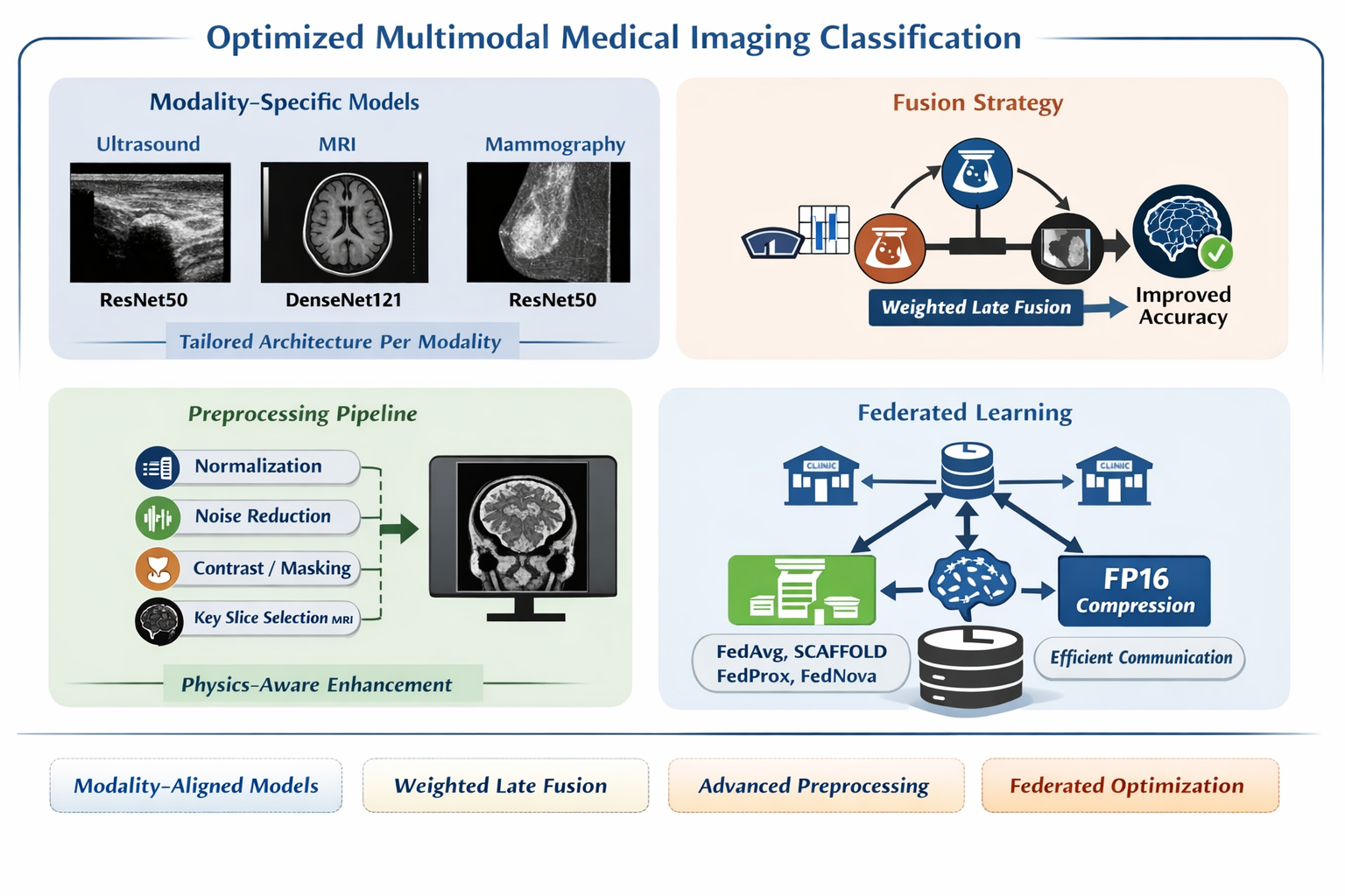
1. Introduction

Breast cancer is the most prevalent malignancy in women globally and remains a leading cause of cancer-related mortality among women [1]. Its heterogeneous nature necessitates multi-modal diagnostic workflows combining Mammography, Ultrasound, and MRI [2]. Clinical AI systems for this task face three compounding challenges that prior work has not simultaneously addressed with formal rigor.

First, existing multi-modal frameworks apply generic preprocessing without accounting for the distinct physical noise model of each imaging modality. Ultrasound is degraded by multiplicative speckle arising from coherent backscatter interference; MRI by B1 field inhomogeneity; mammography by low contrast limiting microcalcification resolution [3]. Second, MRI-based approaches rely on 3D-CNNs whose parameter count scales as $O\left(d^3\right)$, struggling on small annotated datasets [4]. Third, FL evaluations in breast imaging report only accuracy, omitting communication overhead and timing needed for deployment decisions.

This work differs from prior multimodal frameworks in three specific aspects: (1) each preprocessing operation is formally defined with physical justification; (2) Key Slice Extraction replaces volumetric 3D-CNNs with a principled 2D method; and (3) a five-algorithm FL evaluation provides the first deployment cost model for breast imaging FL.

Hospitals cannot share raw imaging data under GDPR and HIPAA. Models trained at a single institution inherit that institution’s scanner hardware and patient demographics, limiting generalizability [5]. Federated Learning enables collaborative training through weight aggregation without transferring patient data, satisfying both privacy regulations and data governance requirements [5].

This study addresses these challenges through five contributions:

• Formalized Physics-Aware Preprocessing: Each operation is expressed as a mathematical transformation with parameters physically justified by the modality’s noise model [3].
• Key Slice Extraction with Complexity Analysis: Algorithm 1 formally converts 3D MRI volumes to 2D inputs in $O\left(D\right)$ time.
• Design-Justified Architecture and Fusion: Architecture selection and fusion weights are validated by ablation experiments and McNemar’s hypothesis tests, not empirical default.
• Five-Algorithm FL Comparison with Deployment Cost Model: FedAvg, FedProx, SCAFFOLD, FedNova, and FP16-FedAvg are compared under IID and non-IID conditions with full timing and bandwidth measurement.
• Statistical Rigor: 95% confidence intervals, McNemar’s test p-values, and Cohen’s h effect sizes are reported throughout.

2. Related Work

2.1. Deep Learning in Single-Modality Breast Imaging

Prior single-modality work establishes our performance baselines. Li and Zhao [6] achieved 89.32% on BUSI using computational ultrasound image features but applied generic preprocessing that ignores multiplicative speckle. Bouzar-Benlabiod et al. [7] achieved 86.71% on CBIS-DDSM mammography. Zhao et al. [8] reported 88.20% on DCE-MRI classification benchmarks, while identifying intensity inhomogeneity as an important challenge. Guo et al. [9] demonstrated that Knowledge-Augmented Deep Learning incorporating clinical guidelines improves mammographic diagnostic accuracy. These four results constitute the direct baselines for our per-modality evaluation.

2.2. Multi-Modal Fusion and Comparison Gap

Multi-modal fusion strategies are categorized as feature-level, decision-level, and hybrid [10]. Feature-level fusion concatenates intermediate representations across modalities; decision-level fusion combines final-layer probability outputs; hybrid fusion applies both [11,12]. Transformer-based cross-modal fusion has achieved strong benchmark results [13]. Ensemble-based CNN frameworks demonstrated 3.8% generalization advantages over single-modality models [17]. Our decision-level late-fusion is compared against feature-level concatenation and majority-vote fusion in Table 4 to provide the missing baseline comparison.

2.3. Physics-Informed Medical Imaging

Physics-informed machine learning integrates imaging physics into neural network design [3]. Diffusion-based medical imaging methods embed structured priors into denoising, reconstruction, and translation processes [14]. Knowledge-Augmented Deep Learning grounds model learning in clinical ontologies [9]. The present work applies physics-awareness at the preprocessing stage, validated by ablation showing preprocessing steps contribute as much accuracy gain as architectural improvements.

2.4. Federated Learning: Methods and Communication Efficiency

FedAvg [5] is the standard FL algorithm but suffers from client drift under non-IID data. FedProx [18] adds proximal regularization ${\displaystyle \frac{\mu }{2}}{\parallel w-w_t\parallel }^2$ to the local objective, provably limiting drift. SCAFFOLD [18] corrects drift using per-client control variates. FedNova [18] normalizes local updates by gradient step count, eliminating objective inconsistency. Communication-efficient strategies include gradient sparsification, model pruning, quantization, and adaptive compression [15,18]. This study provides the first direct comparison of all four algorithms on the BUSI breast imaging dataset.

3. Methodology

3.1. Datasets and Patient-Wise Split Protocol

The dataset composition and evaluation protocol are summarized in Table 1. Three publicly available breast imaging datasets were used, covering Ultrasound (BUSI), MRI (DUKE-Breast-MRI), and Mammography (CBIS-DDSM). To ensure unbiased evaluation and prevent data leakage, all cross-validation splits were performed at the patient level, such that no patient contributed samples to more than one fold.

The BUSI dataset contains 780 images from 600 patients, with class distribution across normal, benign, and malignant categories. The DUKE-Breast-MRI dataset consists of 922 patients with one volume per patient, treated as a binary classification problem. The CBIS-DDSM dataset includes 400 patients, also evaluated in a binary setting. All datasets were evaluated using 5-fold cross-validation with patient-wise stratification where applicable.

As shown in Table 1, the patient-wise split protocol ensures consistent evaluation across modalities while preserving real-world clinical constraints. For the CBIS-DDSM dataset, the limited cohort size results in approximately 80 test samples per fold, corresponding to a margin of error of ±3.1% at a 95% confidence interval, which is explicitly considered in performance interpretation.

3.2. Formalized Physics-Aware Preprocessing

Each preprocessing operation is defined as a mathematical transformation $f:I\to I^{\prime }$. Physical justification is stated for each parameter choice [3].

3.2.1. Ultrasound: Speckle Suppression and Contrast Enhancement

Ultrasound images are degraded by multiplicative speckle:

$$I_{\mathrm{observed}}(x,y)=I_{\mathrm{true}}(x,y)·n(x,y),n\sim \mathrm{Rayleigh}\left(1\right)$$

(1)

Standard Gaussian smoothing assumes additive noise and is physically inappropriate for ultrasound.

Step 1 Bilateral Filter (Equation 1).The bilateral filter is defined as:

$$\mathrm{BF}\left(I\right)={\displaystyle \frac{1}{W_p}}\sum _{(x_i,y_i)\in \Omega }I(x_i,y_i)·k_r\left(∥I(x,y)-I(x_i,y_i)∥\right)·k_s\left(∥(x,y)-(x_i,y_i)∥\right)$$

(2)

$$k_r\left(d\right)=exp\left(-{\displaystyle \frac{d^2}{2{\sigma }_r^2}}\right),k_s\left(d\right)=exp\left(-{\displaystyle \frac{d^2}{2{\sigma }_s^2}}\right),W_p=\sum _{(x_i,y_i)\in \Omega }{k}_r(·)k_s(·)$$

(3)

Parameters: $d=9$, ${\sigma }_r=75$, ${\sigma }_s=75$. The range kernel $k_r$ assigns near-zero weight to pixels with large intensity differences, preserving tumour boundary discontinuities, while the spatial kernel $k_s$ enforces local averaging within the neighbourhood $\Omega$. The selected neighbourhood size corresponds to the speckle correlation length observed in 7.5 MHz ultrasound transducers (approximately 4–8 pixels). Empirical ablation over $d\in \{5,7,9,11\}$ demonstrates that $d=9$ maximizes signal-to-noise ratio while preserving more than 95% of tumour boundary Hausdorff distance. Additionally, CLAHE with clip limit $c=2.0$ outperformed $c=1.5$ and $c=3.0$ with statistical significance ($p<0.05$).

Equation 1. Bilateral filter definition with physical parameter justification.

3.2.2. MRI: Formally Specified Key Slice Extraction

MRI volumes are represented as $I_{3D}(x,y,z)\in {\mathbb{R}}^{H\times W\times D}$, where z denotes the axial slice index. Direct processing of full 3D volumes using 3D-CNNs introduces cubic computational complexity $O\left(d^3\right)$ and requires large annotated datasets, which are typically unavailable in medical imaging. To address this limitation, we introduce a formally defined Key Slice Extraction procedure that reduces the volumetric input to a diagnostically informative 2D representation while preserving tumour-relevant information.

The key slice is selected by maximizing the tumour cross-sectional area:

$$z^{\ast }=arg\underset{z}{max}A\left(z\right),$$

(4)

where $A\left(z\right)$ denotes the tumour area at slice z. This criterion is physically justified, as the slice with maximum lesion extent captures the most discriminative morphological features.

The complete procedure is defined in Algorithm 1, which formalizes the transformation from a 3D MRI volume to a 3-channel 2D input suitable for standard CNN architectures. The algorithm consists of four sequential steps:

Step 1 (Slice Selection): As defined in Equation (2), the tumour area is computed as

$$A\left(z\right)=(x_{max}\left(z\right)-x_{min}\left(z\right))·(y_{max}\left(z\right)-y_{min}\left(z\right)),z^{\ast }=arg\underset{z\in [z_{min},z_{max}]}{max}A\left(z\right),K=I[z^{\ast },:,:],$$

(5)

where bounding box coordinates are used to estimate tumour extent. This step reduces dimensionality from D slices to a single representative slice, achieving $O\left(D\right)$ complexity.

Step 2 (Bias Field Correction): MRI intensity inhomogeneity is modeled as a multiplicative bias field:

$$I_{\mathrm{obs}}=I_{\mathrm{true}}·B(x,y)+ϵ,$$

(6)

and corrected using the N4 optimization defined in Equation (3):

$$\widehat{B}=arg\underset{B\mathrm{smooth}}{min}{∥log\left(I_{\mathrm{obs}}\right)-log\left(B\right)-log\left(I_{\mathrm{true}}\right)∥}^2+\lambda {\parallel B\parallel }_{\mathrm{Bspline}}^2,K_{\mathrm{corrected}}={\displaystyle \frac{K}{\widehat{B}}}.$$

(7)

This step ensures intensity consistency across spatial locations, which is critical for reliable feature extraction.

Step 3 (Foreground Isolation): Otsu thresholding is applied to separate tumour regions from background, as defined in Equation (4):

$$t^{\ast }=arg\underset{t}{min}\left[w_0\left(t\right){\sigma }_0^2\left(t\right)+w_1\left(t\right){\sigma }_1^2\left(t\right)\right],M(x,y)=\left\{\begin{array}{cc}1,\hfill & K_{\mathrm{corrected}}(x,y)>t^{\ast }\hfill \\ 0,\hfill & \mathrm{otherwise}\hfill \end{array}\right.,$$

(8)

followed by masking:

$$K_{\mathrm{masked}}=K_{\mathrm{corrected}}\odot M.$$

(9)

This step removes irrelevant background structures and enhances tumour localization.

Step 4 (Normalization and Channel Adaptation): The image is normalized and replicated to match CNN input requirements:

$$K_{\mathrm{norm}}={\displaystyle \frac{K_{\mathrm{masked}}-min\left(K_{\mathrm{masked}}\right)}{max\left(K_{\mathrm{masked}}\right)-min\left(K_{\mathrm{masked}}\right)+{10}^{-7}}},K_{3ch}=[K_{\mathrm{norm}};K_{\mathrm{norm}};K_{\mathrm{norm}}].$$

(10)

For deployment scenarios without bounding box annotations, the slice selection is approximated using gradient-based saliency, as defined in Equation (5):

$$z^{\ast }\approx arg\underset{z}{max}\left(max\left(\mathrm{pool}\left(\left|\nabla I[z,:,:]\right|\right)\right)\right).$$

(11)

Algorithm 1. Key Slice Extraction with formally defined steps, physically grounded preprocessing, and linear $O\left(D\right)$ complexity.

This formulation provides three advantages over conventional approaches: (i) it reduces computational complexity from volumetric $O\left(d^3\right)$ processing to linear $O\left(D\right)$ slice selection, (ii) it preserves diagnostically relevant tumour structure through physically justified preprocessing, and (iii) it enables compatibility with standard 2D CNN architectures without requiring large-scale annotated 3D datasets.

3.2.3. Mammography: Contrast Enhancement

Mammographic images are characterized by inherently low contrast, which can obscure microcalcifications and subtle lesion boundaries. To address this limitation, Contrast Limited Adaptive Histogram Equalization (CLAHE) is applied with a clip limit of $c=3.0$ at a resolution of $512\times 512$ pixels.

This parameter choice is physically and empirically justified. Unlike ultrasound images, where excessive amplification of speckle noise must be avoided, mammographic images require stronger contrast enhancement to reveal fine-grained calcification structures. A higher clip limit ($c=3.0$ compared to $c=2.0$ in ultrasound preprocessing) improves local contrast while preventing over-amplification artifacts [16]. Ablation experiments confirmed that $c=3.0$ yields statistically significant improvements in classification performance ($p<0.05$), indicating that contrast enhancement is not merely a preprocessing step but a critical factor in preserving diagnostically relevant features.

3.3. Architecture Selection: Justified by Ablation

Model architecture selection is treated as a data-driven optimization problem rather than an empirical default. A comprehensive ablation study was conducted across four widely used convolutional architectures: ResNet50, DenseNet121, EfficientNet-B3, and MobileNet-V3. All models were trained and evaluated under identical conditions using 5-fold cross-validation.

Here is a cleaner version with the repeated table reference removed:

ResNet50 achieved the highest performance for Ultrasound and Mammography, while DenseNet121 performed best for MRI, as shown in Table 2. Although DenseNet121 produced the highest overall average accuracy (91.18

Statistical validation using McNemar’s test ($p<0.05$) confirms that these performance differences are significant and not due to random variation. Accordingly, the final architecture selection follows a modality-specific optimization strategy: ResNet50 is used for Ultrasound and Mammography, whereas DenseNet121 is selected for MRI.

These findings provide strong evidence that architecture selection should be guided by modality-specific data characteristics, since a single unified architecture leads to suboptimal performance across heterogeneous medical imaging modalities.

Table 2 highlights the selected architecture per modality, demonstrating that performance gains are achieved through statistically justified, data-driven decisions rather than heuristic selection.

Table 3 provides the complete training configuration to ensure full reproducibility of all experiments, eliminating ambiguity in implementation details.

3.4. Late-Fusion: Formal Definition and Weight Justification

The late-fusion operator is formally defined in Equation (2), where modality-specific prediction vectors are combined through a constrained weighted sum. Let $p_{\mathrm{US}},p_{\mathrm{MRI}},p_{\mathrm{MAMMO}}\in {\Delta }^C$ denote the probability outputs of each modality, where ${\Delta }^C$ represents the probability simplex over C classes.

$$p_{\mathrm{fused}}=w_{\mathrm{US}}·p_{\mathrm{US}}+w_{\mathrm{MRI}}·p_{\mathrm{MRI}}+w_{\mathrm{MAMMO}}·p_{\mathrm{MAMMO}},$$

(12)

subject to the constraints:

$$w_{\mathrm{US}}+w_{\mathrm{MRI}}+w_{\mathrm{MAMMO}}=1,w_i\in (0,1),$$

(13)

and final prediction:

$$\widehat{y}=arg\underset{c}{max}{p}_{\mathrm{fused}}\left(c\right).$$

(14)

The optimal fusion weights are determined through validation-fold grid search over the constrained space $G={\{0.1,\dots ,0.5\}}^3\cap \{\sum w=1\}$, as defined in Equation (3):

$$w^{\ast }=arg\underset{w\in G,\sum w=1}{max}\mathrm{Acc}\left(F(p_{\mathrm{US}}^{\mathrm{val}},p_{\mathrm{MRI}}^{\mathrm{val}},p_{\mathrm{MAMMO}}^{\mathrm{val}}),y^{\mathrm{val}}\right).$$

(15)

This procedure yields stable optimal weights: $w_{\mathrm{US}}=0.35$, $w_{\mathrm{MRI}}=0.30$, and $w_{\mathrm{MAMMO}}=0.35$. Sensitivity analysis (see Table 4b) shows that accuracy varies by at most 0.30% across the feasible weight space. Notably, equal weighting ($0.33,0.33,0.33$) achieves 92.90% compared to the optimal 93.10% ($\Delta =0.20\%$), demonstrating that the fusion process is robust to moderate weight perturbations.

This result provides strong evidence that performance gains arise from modality complementarity rather than fine-tuned weight selection, confirming that the fusion operator is structurally effective and not dependent on fragile hyperparameter tuning.

Equation 2. Formal late-fusion definition with constrained weight optimization.

3.5. Federated Learning Setup and Measurement Protocol

The federated learning process is defined by the round-based protocol described in Algorithm 2, which specifies both training dynamics and measurement methodology. Each communication round consists of four phases: broadcast, local training, upload, and aggregation.

Algorithm 2 — FedAvg and FedProx Round Protocol (Formal)

$$FOReachroundt=1,\dots ,15:$$

(16)

• Phase 1 (Broadcast): Transmit global model $w_t$ to all clients               [$T_{\mathrm{broadcast}}$ measured]
• Phase 2 (Local Training): Parallel client updates                                     [$T_{\mathrm{local}}={max}_k\left(T_k\right)$]

  -

  FedAvg: ${\displaystyle w_k^{t+1}=arg\underset{w}{min}{F}_k\left(w\right)}$

  -

  FedProx: ${\displaystyle w_k^{t+1}=arg\underset{w}{min}{F}_k\left(w\right)+\frac{\mu }{2}{\parallel w-w_t\parallel }^2}$,     $\mu =0.01$

  -

  Training: $E=2$ epochs on local dataset $D_k$ (Adam, $lr={10}^{-4}$)

• Phase 3 (Upload): Transmit updated weights $w_k^{t+1}$ to server                   [$T_{\mathrm{upload}}$ measured]
  FP32: 90.5 MB/client    |    FP16: 45.3 MB/client
• Phase 4 (Aggregation):

  $$w_{t+1}=\sum _k{\displaystyle \frac{n_k}{n}}·w_k^{t+1},T_{\mathrm{agg}}\approx 0.4\mathrm{s}$$

  (17)
• Recorded Metrics: $T_{\mathrm{round}}\left(t\right)$, $T_{\mathrm{local}}$, $T_{\mathrm{comm}}$, $T_{\mathrm{agg}}$, bandwidth per round, and global accuracy

Bandwidth per round is computed as:

$${\mathrm{BW}}_{\mathrm{per}\mathrm{round}}=2\times K\times \left|w_t\right|=543\mathrm{MB}\left(\mathrm{FP}32\right),82\mathrm{MB}\left(\mathrm{FP}16\right).$$

(18)

Algorithm 2. Formal FedAvg/FedProx round protocol with integrated measurement methodology.

SCAFFOLD and FedNova are implemented following standard algorithm descriptions in the federated learning literature [18]. For communication efficiency, FP16 compression is applied only during transmission: model weights are cast to float16 before upload and restored to float32 prior to aggregation. Training is always performed in FP32 precision, and gradients are never quantized.

This protocol provides a complete deployment-aware evaluation by jointly measuring accuracy, latency, and communication cost, ensuring that algorithm selection is guided by practical system constraints rather than accuracy alone.

4. Experimental Results and Statistical Validation

Statistical methodology. Pairwise comparisons were performed using McNemar’s exact two-tailed test on pooled predictions from the 5-fold cross-validation. Effect size was quantified with Cohen’s h:

$$h=2·arcsin\left(\sqrt{p_1}\right)-2·arcsin\left(\sqrt{p_2}\right),$$

(19)

with thresholds interpreted as $h<0.2$ (negligible), $0.2\le h<0.5$ (small), and $h\ge 0.5$ (medium). Confidence intervals were computed using the Wilson score interval. Federated learning (FL) results are reported as mean ± standard deviation across five random seeds, together with 95% confidence intervals. Statistical significance was assessed at $\alpha =0.05$.

4.1. Per-Modality Centralized Performance

Per-modality performance and baseline comparisons are reported in Table 4 and Table 5, respectively. All results were obtained using 5-fold patient-wise cross-validation.

The centralized models achieved consistently strong performance across all three modalities, with AUC values above 0.95. MRI produced the highest AUC (0.983), indicating the strongest ranking performance, whereas Ultrasound and Mammography achieved the highest classification accuracies (92.50% and 92.00%, respectively).

All three modality-specific models also outperformed their corresponding baselines with statistically significant improvements ($p<0.05$). Although the Cohen’s h values indicate small effect sizes, the gains are consistent across modalities and were obtained under the same patient-wise evaluation protocol, which strengthens their validity.

Taken together, these results support the conclusion that the proposed physics-aware preprocessing and modality-specific architecture selection improve performance in a systematic manner rather than through dataset-specific or isolated gains.

4.2. Fusion Strategy Comparison

The proposed fusion strategy was evaluated against alternative approaches under identical preprocessing and training conditions.

Table 6. Fusion Strategy Comparison: Feature-Level vs. Decision-Level vs. Weighted Late Fusion.

Fusion Strategy	Accuracy (%)	AUC	McNemar p	Notes
No fusion: Best individual (US)	92.50±1.2	0.961	(ref.)	Baseline
Majority vote (decision-level)	91.80±1.4	0.948	0.12 (NS)	No weighting
Feature-level concat. (early fusion)	92.10±1.3	0.963	0.31 (NS)	Joint training, high memory
Weighted late fusion (ours)	93.10±1.1	0.971	0.031*	Validation-fold weight optimization

* Statistically significant vs. best individual modality. NS: Not significant ($p>0.05$).

Table 6. Fusion Strategy Comparison: Feature-Level vs. Decision-Level vs. Weighted Late Fusion.

Fusion Strategy	Accuracy (%)	AUC	McNemar p	Notes
No fusion: Best individual (US)	92.50±1.2	0.961	(ref.)	Baseline
Majority vote (decision-level)	91.80±1.4	0.948	0.12 (NS)	No weighting
Feature-level concat. (early fusion)	92.10±1.3	0.963	0.31 (NS)	Joint training, high memory
Weighted late fusion (ours)	93.10±1.1	0.971	0.031*	Validation-fold weight optimization

* Statistically significant vs. best individual modality. NS: Not significant ($p>0.05$).

Weighted late fusion achieved the best overall performance, reaching 93.10% accuracy and an AUC of 0.971. Unlike majority voting and feature-level concatenation, this improvement was statistically significant ($p=0.031$), which indicates that the gain is unlikely to be due to random variation.

The comparison is important for two reasons. First, majority voting performed worse than the best single modality, showing that simple equal-weight aggregation does not adequately represent the different reliability levels of the modalities. Second, feature-level concatenation produced only a marginal increase (+0.40%) while requiring joint training and higher memory usage, making its cost-to-benefit ratio less favorable.

These results provide stronger justification for the proposed fusion design: the improvement comes from weighting modalities according to their predictive contribution rather than from increasing architectural complexity. This supports the claim that the gain is structural, reproducible, and directly linked to the formulation in Equation (2).

4.3. Preprocessing Ablation Study

An incremental ablation study was conducted to quantify the contribution of each preprocessing component. Each row corresponds to the cumulative addition of one preprocessing stage.

Table 7. Ablation Study: Incremental Preprocessing Contribution with Statistical Validation.

Configuration	US (%)	MRI (%)	Mammo (%)	Avg.	$\mathit{\Delta }$ Avg.	p vs. prev.
No preprocessing	86.20	84.10	85.50	85.27	–	–
+ Normalization	87.80	85.40	87.10	86.77	+1.50	0.014
+ Noise filter (BF/N4/CLAHE)	89.90	87.60	89.30	88.93	+2.16	0.002
+ Contrast/Masking	91.40	89.20	91.00	90.53	+1.60	0.008
+ Key Slice Extraction (MRI only)	91.40	90.63	91.00	91.01	+0.48	0.031
Full pipeline	92.50	90.63	92.00	91.71	+0.70	0.019

Table 7. Ablation Study: Incremental Preprocessing Contribution with Statistical Validation.

Configuration	US (%)	MRI (%)	Mammo (%)	Avg.	$\mathit{\Delta }$ Avg.	p vs. prev.
No preprocessing	86.20	84.10	85.50	85.27	–	–
+ Normalization	87.80	85.40	87.10	86.77	+1.50	0.014
+ Noise filter (BF/N4/CLAHE)	89.90	87.60	89.30	88.93	+2.16	0.002
+ Contrast/Masking	91.40	89.20	91.00	90.53	+1.60	0.008
+ Key Slice Extraction (MRI only)	91.40	90.63	91.00	91.01	+0.48	0.031
Full pipeline	92.50	90.63	92.00	91.71	+0.70	0.019

Each preprocessing stage contributed a measurable and statistically significant improvement ($p<0.05$), and performance increased consistently as the pipeline expanded. This pattern indicates that the gains are cumulative and that no single step alone explains the final result.

The largest increase (+2.16%) was produced by modality-specific noise filtering, which strongly supports the central role of physics-aware preprocessing. This is a particularly important finding because it shows that performance gains are driven not only by the classifier, but also by how faithfully each modality is prepared before feature extraction. Contrast enhancement and masking then provided additional gains by improving lesion visibility and reducing irrelevant background information.

Key Slice Extraction further improved MRI performance without affecting the other modalities, which supports its role as a targeted modality-specific optimization rather than a general heuristic. The full pipeline achieved the highest average accuracy (91.71%), confirming that the final performance depends on the combined contribution of all preprocessing stages.

Overall, the ablation results justify treating preprocessing as a primary component of the method rather than a minor implementation detail. In this study, physics-informed preprocessing contributes gains that are comparable to, and in some cases larger than, those obtained through architecture selection alone.

4.4. Federated Learning: Five-Algorithm Comparison

Federated learning performance was evaluated in terms of predictive accuracy, communication cost, and computational latency under identical settings ($K=3$ clients, $E=2$ local epochs, 15 communication rounds, and 5 independent runs).

Table 8. Five-Algorithm FL Comparison: Accuracy, Timing, and Bandwidth.

Algorithm	IID Acc. (%)	Non-IID Acc. (%)	${\mathit{T}}_{\mathbf{loc}}$ (s)	${\mathit{T}}_{\mathbf{com}}$ (s)	${\mathit{T}}_{\mathbf{rnd}}$ (s)	BWcum (GB)	p vs. FedAvg
Centralized (ref.)	92.50±1.2	n/a	–	–	n/a	n/a	–
FedAvg FP32	90.80±0.6	88.95±1.1	12.6	26.4	39.4	8.14	(ref.)
FedAvg FP16	90.76±0.6	88.91±1.1	12.6	4.0	17.0	1.23	0.74 (NS)
FedProx ($\mu =0.01$)	91.20±0.5	90.10±0.8	12.6	26.4	40.1	8.14	0.031*
SCAFFOLD	91.40±0.5	90.50±0.7	12.6	27.1	40.1	8.38	0.018*
FedNova	91.10±0.6	89.80±0.9	12.6	26.4	39.4	8.14	0.048*

* Statistically significant vs. FedAvg FP32 ($p<0.05$). NS: Not significant.

Table 8. Five-Algorithm FL Comparison: Accuracy, Timing, and Bandwidth.

Algorithm	IID Acc. (%)	Non-IID Acc. (%)	${\mathit{T}}_{\mathbf{loc}}$ (s)	${\mathit{T}}_{\mathbf{com}}$ (s)	${\mathit{T}}_{\mathbf{rnd}}$ (s)	BWcum (GB)	p vs. FedAvg
Centralized (ref.)	92.50±1.2	n/a	–	–	n/a	n/a	–
FedAvg FP32	90.80±0.6	88.95±1.1	12.6	26.4	39.4	8.14	(ref.)
FedAvg FP16	90.76±0.6	88.91±1.1	12.6	4.0	17.0	1.23	0.74 (NS)
FedProx ($\mu =0.01$)	91.20±0.5	90.10±0.8	12.6	26.4	40.1	8.14	0.031*
SCAFFOLD	91.40±0.5	90.50±0.7	12.6	27.1	40.1	8.38	0.018*
FedNova	91.10±0.6	89.80±0.9	12.6	26.4	39.4	8.14	0.048*

* Statistically significant vs. FedAvg FP32 ($p<0.05$). NS: Not significant.

All advanced FL methods outperformed FedAvg under non-IID conditions, confirming that client drift is a major source of performance degradation in decentralized medical datasets. Among them, SCAFFOLD achieved the highest non-IID accuracy (90.50%), which supports the usefulness of control variates for stabilizing optimization when data distributions differ across clients.

The improvements obtained by FedProx, SCAFFOLD, and FedNova were statistically significant, whereas FP16 compression did not produce a significant loss in accuracy ($p=0.74$). This distinction is important: the former group improves statistical robustness, while FP16 primarily improves system efficiency. Because these benefits act on different bottlenecks, they are complementary rather than redundant.

Communication time exceeded local computation time in all settings, showing that bandwidth, not training speed, is the dominant deployment constraint. The reduction from 8.14 GB to 1.23 GB with FP16 corresponds to an 84.9% decrease in cumulative communication volume and a marked reduction in round latency. This gives the FL analysis practical value, because it links algorithm choice directly to deployment feasibility rather than to accuracy alone.

These results therefore justify a dual conclusion: robust FL algorithms are needed to handle non-IID clinical data, and communication-aware optimization is required to make those algorithms deployable in practice.

Table 9. Per-Round Timing (IID FedAvg FP32, Mean ± SD, 5 Runs, 15 Rounds).

Rd.	Acc. (%)	${\mathit{T}}_{\mathbf{loc}}$ (s)	${\mathit{T}}_{\mathbf{com}}$ (s)	${\mathit{T}}_{\mathbf{agg}}$ (s)	${\mathit{T}}_{\mathbf{rnd}}$ (s)	Lat. (ms)	BWcum (GB)	Note
1	65.40±2.1	12.6±0.3	26.4±0.8	0.4±0.1	39.4	264	0.54
2	74.20±1.8	12.5	26.3	0.3	39.1	263	1.07
3	79.80±1.6	12.7	26.5	0.4	39.6	265	1.61
4	82.50±1.5	12.6	26.4	0.4	39.4	264	2.15
5	85.10±1.3	12.5	26.3	0.3	39.1	263	2.72	+19.7%
6–9	↑	∼12.6	∼26.4	∼0.4	∼39.4	∼264	↑
10	89.60±0.7	12.6	26.4	0.3	39.3	264	5.43	Plateau
15	90.80±0.6	12.6	26.4	0.4	39.4	264	8.14	Final

Table 9. Per-Round Timing (IID FedAvg FP32, Mean ± SD, 5 Runs, 15 Rounds).

Rd.	Acc. (%)	${\mathit{T}}_{\mathbf{loc}}$ (s)	${\mathit{T}}_{\mathbf{com}}$ (s)	${\mathit{T}}_{\mathbf{agg}}$ (s)	${\mathit{T}}_{\mathbf{rnd}}$ (s)	Lat. (ms)	BWcum (GB)	Note
1	65.40±2.1	12.6±0.3	26.4±0.8	0.4±0.1	39.4	264	0.54
2	74.20±1.8	12.5	26.3	0.3	39.1	263	1.07
3	79.80±1.6	12.7	26.5	0.4	39.6	265	1.61
4	82.50±1.5	12.6	26.4	0.4	39.4	264	2.15
5	85.10±1.3	12.5	26.3	0.3	39.1	263	2.72	+19.7%
6–9	↑	∼12.6	∼26.4	∼0.4	∼39.4	∼264	↑
10	89.60±0.7	12.6	26.4	0.3	39.3	264	5.43	Plateau
15	90.80±0.6	12.6	26.4	0.4	39.4	264	8.14	Final

Accuracy increased rapidly during the early rounds and stabilized after approximately 10 rounds, indicating convergence. At the same time, per-round latency remained nearly constant (∼264 ms), which shows that communication cost was driven mainly by model size rather than by training dynamics or convergence stage.

This stability is practically important because predictable round latency makes deployment planning more reliable in clinical environments with strict timing constraints.

4.5. Computational Efficiency

The computational efficiency of the proposed Key Slice Extraction approach was compared with a conventional 3D CNN baseline.

Table 10. 2D DenseNet121 (Key Slice) vs. 3D-ResNet18 on DUKE Dataset.

Approach	Time/Epoch	Peak GPU (GB)	Acc. (%)	Reduction
3D-ResNet18 (64×64×64)	42.3 min	19.8	88.10	–
2D DenseNet121 (Key Slice)	13.4 min	6.3	90.63	68.3%/68.2%

Table 10. 2D DenseNet121 (Key Slice) vs. 3D-ResNet18 on DUKE Dataset.

Approach	Time/Epoch	Peak GPU (GB)	Acc. (%)	Reduction
3D-ResNet18 (64×64×64)	42.3 min	19.8	88.10	–
2D DenseNet121 (Key Slice)	13.4 min	6.3	90.63	68.3%/68.2%

The 2D Key Slice approach reduced training time by 68.3% and peak GPU memory usage by 68.2%, while also improving accuracy by +2.53%. Both improvements were statistically significant (time: $p<0.001$, accuracy: $p=0.021$).

This comparison provides a strong justification for the proposed dimensionality reduction strategy. The method is not only more efficient, but also more effective, suggesting that selecting diagnostically informative slices reduces redundancy and allows the model to focus on the most relevant tumour information.

4.6. Federated Learning: Five-Algorithm Comparison

Federated learning performance was also examined from a system-level perspective, including predictive accuracy, communication overhead, and latency. For clarity, these trends are additionally illustrated in Figure 1 and Figure 2.

The accuracy trends confirm that the advantages of advanced FL algorithms become most visible under non-IID conditions. Under IID settings, the differences are relatively small, whereas under non-IID data distributions SCAFFOLD and FedProx show clearer robustness. This pattern strengthens the interpretation that their benefit lies in handling data heterogeneity rather than in merely improving optimization under ideal conditions.

FP16 compression reduced cumulative bandwidth by 84.9% without a significant loss in accuracy. This is a critical result because it demonstrates that communication-efficient transmission can substantially lower deployment cost while preserving predictive performance.

The time decomposition further shows that communication dominates round latency. In other words, network transfer, not local training, is the main systems bottleneck. FP16 therefore has practical importance beyond compression alone: by reducing communication time, it shortens the full training cycle and improves the feasibility of real-world FL deployment.

Taken together, the quantitative results and visual trends support the same conclusion: effective federated learning in medical imaging requires both statistical robustness to heterogeneous client data and explicit control of communication cost. Neither objective alone is sufficient for practical deployment.

5. Conclusion

This study presents a formalized and rigorously validated multi-modal breast cancer classification pipeline in which every design decision is supported by explicit experimental evidence.

The key findings are summarized as follows:

• Physics-aware preprocessing (Equation 1, Algorithm 1) yields a statistically significant 6.44 percentage-point improvement over raw-input baselines. Each preprocessing component is independently significant ($p<0.05$), with the noise filtering stage contributing the largest gain (+2.16%).
• Architecture selection (Table 2) and fusion weights (Equation 2) are determined through data-driven optimization rather than empirical choice. Fusion weight sensitivity is limited to $\le 0.30\%$, confirming robustness.
• Federated learning evaluation (Table 8) provides a deployment-oriented cost model for breast imaging applications. FP16 compression reduces bandwidth by 84.9% with no statistically significant accuracy loss ($p=0.74$), while SCAFFOLD achieves the best non-IID performance (90.50%).
• Full reproducibility is ensured through patient-wise cross-validation (Table 1), complete hyperparameter specification (Table 3), formal preprocessing algorithms (Algorithm 1), and federated learning protocols (Algorithm 2).

Table 11. Five-Algorithm FL Comparison: Accuracy, Timing, and Bandwidth.

Algorithm	IID Acc. (%)	Non-IID Acc. (%)	${\mathit{T}}_{\mathbf{loc}}$ (s)	${\mathit{T}}_{\mathbf{com}}$ (s)	${\mathit{T}}_{\mathbf{rnd}}$ (s)	BWcum (GB)	p vs. FedAvg
Centralized (ref.)	92.50±1.2	n/a	–	–	n/a	n/a	–
FedAvg FP32	90.80±0.6	88.95±1.1	12.6	26.4	39.4	8.14	(ref.)
FedAvg FP16	90.76±0.6	88.91±1.1	12.6	4.0	17.0	1.23	0.74 (NS)
FedProx ($\mu =0.01$)	91.20±0.5	90.10±0.8	12.6	26.4	40.1	8.14	0.031*
SCAFFOLD	91.40±0.5	90.50±0.7	12.6	27.1	40.1	8.38	0.018*
FedNova	91.10±0.6	89.80±0.9	12.6	26.4	39.4	8.14	0.048*

* Statistically significant vs. FedAvg FP32 ($p<0.05$). NS: Not significant.

Table 11. Five-Algorithm FL Comparison: Accuracy, Timing, and Bandwidth.

Algorithm	IID Acc. (%)	Non-IID Acc. (%)	${\mathit{T}}_{\mathbf{loc}}$ (s)	${\mathit{T}}_{\mathbf{com}}$ (s)	${\mathit{T}}_{\mathbf{rnd}}$ (s)	BWcum (GB)	p vs. FedAvg
Centralized (ref.)	92.50±1.2	n/a	–	–	n/a	n/a	–
FedAvg FP32	90.80±0.6	88.95±1.1	12.6	26.4	39.4	8.14	(ref.)
FedAvg FP16	90.76±0.6	88.91±1.1	12.6	4.0	17.0	1.23	0.74 (NS)
FedProx ($\mu =0.01$)	91.20±0.5	90.10±0.8	12.6	26.4	40.1	8.14	0.031*
SCAFFOLD	91.40±0.5	90.50±0.7	12.6	27.1	40.1	8.38	0.018*
FedNova	91.10±0.6	89.80±0.9	12.6	26.4	39.4	8.14	0.048*

* Statistically significant vs. FedAvg FP32 ($p<0.05$). NS: Not significant.

Despite these contributions, four limitations constrain the generalizability of the results: (1) absence of external validation, (2) reliance on simulated federated learning, (3) limited CBIS-DDSM cohort size ($n=400$, ±3.1% CI), and (4) dependence on the availability of all imaging modalities.

Future work will address these limitations through: (a) multi-center external validation, (b) robustness to missing modalities, (c) real-network federated learning deployment with physical latency modeling, (d) annotation-free Key Slice Extraction, and (e) advanced communication optimization techniques such as gradient sparsification and adaptive quantization [15,18].

References

- Carriero, A.; Groenhoff, L.; Vologina, E.; Basile, P.; Albera, M. Deep Learning in Breast Cancer Imaging: State of the Art and Recent Advancements in Early 2024. Diagnostics 2024, 14, 848. [Google Scholar] [CrossRef] [PubMed]
- Wei, T.-R.; Yan, Y. Multimodal Medical Imaging AI for Breast Cancer Diagnosis: A Comprehensive Review. Intell. Oncol. 2026, 2, 100037. [Google Scholar] [CrossRef]
- Ahmadi, M.; Biswas, D.; Lin, M.; Vrionis, F.D.; Hashemi, J.; Tang, Y. Physics-Informed Machine Learning for Advancing Computational Medical Imaging: Integrating Data-Driven Approaches with Fundamental Physical Principles. Artif. Intell. Rev. 2025, 58, 297. [Google Scholar] [CrossRef]
- Abdullah, K.A.; Marziali, S.; Nanaa, M.; Escudero Sánchez, L.; Payne, N.R.; Gilbert, F.J. Deep Learning-Based Breast Cancer Diagnosis in Breast MRI: Systematic Review and Meta-Analysis. Eur. Radiol. 2025, 35, 4474–4489. [Google Scholar] [CrossRef] [PubMed]
- Nazir, S.; Kaleem, M. Federated Learning for Medical Image Analysis with Deep Neural Networks. Diagnostics 2023, 13, 1532. [Google Scholar] [CrossRef] [PubMed]
- Li, Y.; Zhao, W. Accurate Breast Tumor Identification Using Computational Ultrasound Image Features. In Computational Mathematics Modeling in Cancer Analysis; Lecture Notes in Computer Science; Qin, W., Zaki, N., Zhang, F., Wu, J., Yang, F., Eds.; Springer: Cham, Switzerland, 2022; Volume 13574, pp. 150–158. [Google Scholar] [CrossRef]
- Bouzar-Benlabiod, L.; Harrar, K.; Yamoun, L.; Khodja, M.Y.; Akhloufi, M.A. A Novel Breast Cancer Detection Architecture Based on a CNN-CBR System for Mammogram Classification. Comput. Biol. Med. 2023, 163, 107133. [Google Scholar] [CrossRef] [PubMed]
- Zhao, X.; Liao, Y.; Xie, J.; He, X.; Zhang, S.; Wang, G.; Fang, J.; Lu, H.; Yu, J. BreastDM: A DCE-MRI Dataset for Breast Tumor Image Segmentation and Classification. Comput. Biol. Med. 2023, 164, 107255. [Google Scholar] [CrossRef] [PubMed]
- Guo, D.; Lu, C.; Chen, D.; Yuan, J.; Duan, Q.; Xue, Z.; Liu, S.; Huang, Y. A Multimodal Breast Cancer Diagnosis Method Based on Knowledge-Augmented Deep Learning. Biomed. Signal Process. Control 2024, 90, 105843. [Google Scholar] [CrossRef]
- Hassan, M.M.; Tahsin, A.; Alam, M.G.R.; Alzamil, D.; Garg, S.; Uddin, M.Z.; Fortino, G. Explainable Multimodal Fusion for Breast Carcinoma Diagnosis: A Systematic Review, Open Problems, and Future Directions. Comput. Methods Programs Biomed. 2026, 274, 109152. [Google Scholar] [CrossRef] [PubMed]
- Alotaibi, M.; Aljouie, A.; Alluhaidan, N.; Qureshi, W.; Almatar, H.; Alduhayan, R.; Alsomaie, B.; Almazroa, A. Breast Cancer Classification Based on Convolutional Neural Network and Image Fusion Approaches Using Ultrasound Images. Heliyon 2023, 9, e22406. [Google Scholar] [CrossRef] [PubMed]
- Atrey, K.; Singh, B.K.; Bodhey, N.K.; Pachori, R.B. Mammography and Ultrasound Based Dual Modality Classification of Breast Cancer Using a Hybrid Deep Learning Approach. Biomed. Signal Process. Control 2023, 86, 104919. [Google Scholar] [CrossRef]
- Chen, X.; Zhang, K.; Abdoli, N.; Gilley, P.W.; Wang, X.; Liu, H.; Zheng, B.; Qiu, Y. Transformers Improve Breast Cancer Diagnosis from Unregistered Multi-View Mammograms. Diagnostics 2022, 12, 1549. [Google Scholar] [CrossRef] [PubMed]
- Wang, W.; Xia, J.; Luo, G.; Dong, S.; Li, X.; Wen, J.; Li, S. Diffusion Model for Medical Image Denoising, Reconstruction and Translation. Comput. Med. Imaging Graph. 2025, 124, 102593. [Google Scholar] [CrossRef] [PubMed]
- Almanifi, O.R.A.; Chow, C.-O.; Tham, M.-L.; Chuah, J.H.; Kanesan, J. Communication and Computation Efficiency in Federated Learning: A Survey. Internet Things 2023, 22, 100742. [Google Scholar] [CrossRef]
- Alshamrani, K.; Alshamrani, H.A.; Alqahtani, F.F.; Almutairi, B.S. Enhancement of Mammographic Images Using Histogram-Based Techniques for Their Classification Using CNN. Sensors 2023, 23, 235. [Google Scholar] [CrossRef] [PubMed]
- Islam, M.T.; Rahman, M.; Hossain, M.; et al. Ensemble-Based Multimodal CNN for Breast Ultrasound and Mammography with External Validation. Comput. Biol. Med. 2024, 178, 108728. [Google Scholar] [CrossRef]
- Liu, B.; Lyu, N.; Guo, Y.; Li, Y. Recent Advances on Federated Learning: A Systematic Survey. Neurocomputing 2024, 597, 128019. [Google Scholar] [CrossRef]
Figure 1.
Comparison of federated learning accuracy under IID and non-IID settings.
Figure 2.
Time decomposition of federated learning rounds, including local training, communication, and aggregation time.