Submitted:
13 April 2026
Posted:
14 April 2026
You are already at the latest version
Abstract
In this work, the development and validation of an AI- and sensor-based inline quality monitoring system for the analysis of particle size distributions (PSDs) of comminuted construction and demolition waste (CDW) material flows are described. In this, a custom-developed multitask CNN (CDW-MT-CNN) was developed using manually sieve analyzed particles. This model is able to rapidly and simultaneously predict the particle class and weight, essential for the determination of the PSD. The single particle data are then aggregated per raw image, usually consisting of around 1000 particles for full-scale experiments, to acquire a per-image PSD. The inline mounted RGB line scan sensor records high-resolution images in subsecond frequencies. With an inference time of around 54 ms for a single image, this model would be able to provide a PSD every minute in a full-scale plant. For the purpose of inline monitoring of CDW material flows in a comminution process, such intervals are sufficient according to experts and solves existing gaps regarding the upscaling of laboratory-developed systems. Together with the high predictive performance of the model, especially in terms of classification, it is shown that this technology has potential for monitoring in full-scale plants, for instance by offering operators new insights to improve operation efficiency. Further research should focus on increasing the precision for weight prediction, for instance by increasing the labeled data set with a larger number of unique particles and on methods to verify the performance of the model on pilot or full-scale plants during live operation.
Keywords:
multitask-CNN
; 2D-based material characterization
; particle size distribution
; construction and demolition waste
; inline sensor-based material flow characterization
; recycled concrete aggregates
1. Introduction
Across the European continent, trends indicating increasing demands for construction and building materials are visible, rendering innovations for the improvement of material sustainability within the construction sector — in particular regarding high-grade recycling — a European concern [1,2]. In Germany, the increase in the number of building permits for residential construction in 2020 (+2.2%) and 2021 (+4.8%) [3], renovation of 40,000 dwellings by 2026 [4] and the government’s goal to build 400,000 new dwellings annually [5] show the considerable potential for increased high-grade use of recycled CDW materials. Given that in 2022 nearly 24 million tons of construction and demolition waste (CDW) were generated and forwarded to Germany’s 2.676 CDW processing facilities [6], corresponding to approximately 30 wt% of the generated CDW from Germany’s construction sector [1], a considerable material stream for the production of high-quality recycled aggregates is already established but further potential exists in increasing the amount of material being recycled.
To this day, however, monitoring the quality of the material in CDW processing remains a procedure reliant on manual sampling, despite the inherent lack of transparency regarding material specifications and the material stream characteristics that occur due to limitations of manual sampling. Nonetheless, in recent years there has been an increasing interest in automating material specification analyses, for instance as a basis for assessing the usability of CDW recycled aggregates as a substitute for primary raw materials in high-quality applications such as structural engineering [7] and road construction [8]. In a previous study, we found that research on automating material specification analyses in CDW processing mainly takes place on lower technology readiness levels (TRLs)[9]. This is among other things due to a general lack of labeled data needed for the development of supervised deep learning architectures, the lack of testing in realistic environments and related to this, the complexity of CDW material streams. Additionally, similar to other waste streams (e.g. [10]), several quality factors on the particle or material flow level are based on the weight of the particle or flow, which is difficult to extract from 2D-based sensor data [11]. Alternatively, the use of 3D sensing technologies, such as 3D-laser triangulation, could be used [12,13,14], but given the severe economic constraints and rough environments concerning CDW processing [15,16,17], this currently remains practically infeasible.
To improve the use of CDW recycled aggregates in high-quality applications by increasing the transparency of the material specifications during processing while keeping the costs of the automation technology low, a combination of 2D sensing and deep learning appears to be a suitable strategy. Such a technology can have several benefits, including higher transparency and data richness required for detailed and therewith more trustworthy certification, which could incentivize the use of higher rates of recycled aggregates in construction. Moreover, the increased transparency in combination with real-time results would allow plant operators to efficiently adjust operating parameters to maximize the quality of the produced recyclates, allowing use a wider and qualitatively higher range of application areas. In this context, the particle size distribution (PSD) seems to be one of the most appropriate quality factors: not only is it one of several essential indicators of the CDW material quality, but it is also partially comprised of 2D data that can be extracted using 2D sensing technologies. That is, the particle size distribution represents the cumulative weight percentage of particles classified by their size. However, this still means that, based on the 2D particle class data, an accurate approximation of the weight needs to be made. In the context of CDW, this remains an unsolved problem to this day [18].
1.1. Related Work
Complementary metal-oxide-semiconductor (CMOS) sensors recording 2D RGB data have already shown promising results for primary materials such as glass bead characterization on a m scale [19] and solids during air flow-based transportation in pipes [20]. A first approach for the particle size classification of CDW material was provided by Di Maria et al. in 2016, who proposed and implemented a so-called `look-up catalogue’ procedure [11]. This procedure is however not directly applicable for in- or online quality monitoring during processing because of the lack of a real-time recording and analysis system, but it could be used as a baseline, given a sufficient number of mixture scenarios and different size distributions are provided.
As indicated in the work by Di Maria et al, having sufficient labeled data is imminent for good predictive performance but time-consuming and costly for CDW given the large variety of particles in terms of sizes, shapes and material compositions. As such, to this day no large and labeled data sets for (single) CDW particles exist that could be used for the training of deep learning models for the prediction of the PSD. However, some approaches of how the limitations acquiring suitable CDW image data have been proposed. For instance, [21] describe how synthetic data with different occlusion rates can be created using two distinct types of particles: instances of brick and sand-lime stone. Additionally, [22] use data augmentation to increase the limited data set of 45 photographed particles and train models for the classification of particle shape.
1.2. Aims and Research Questions
The relevance of this work is two-fold. On the one hand, we aim to develop a kind of model not previously used for the prediction of particle size distribution — namely a multitask-CNN, to provide a first attempt at solving the problem of translating 2D information to weight data for particles where no standard material density can be assumed. On the other hand, we aim to mitigate large gaps that exist between models developed on a laboratory scale and the actual practical prerequisites by adapting a bottom-up approach of using practical experiences for the development of a model that is in its basis implementable in real CDW processing environments. As such we also tested the model using full-scale plant data and describe resulting implications. Correspondingly, in this work, the following two research questions will be answered:
RQ1: To what extent can particle size classes and particle weight using only a limited set of 2D-RGB data be predicted with sufficient efficiency, both regarding speed and predictive performance, to meet the practical requirements for the CDW comminution process?
RQ2: How does the proposed solution from RQ1 perform as part of the developed quality monitoring system when applied on full-scale plant data and what are the implications for a full-fledged implementation in a full-scale plant?
2. Materials and Methods
2.1. Materials and Sample Preparation
2.1.1. Sampling Campaign
In order to develop the quality monitoring system and corresponding experiments, acquisition of real CDW material is necessary. Given the heterogeneity of CDW, we conducted multiple sampling campaigns, separated by long time frames (i.e. 4-6 months between each campaign) at the same processing plant, located in North Rhine-Westphalia, Germany. The first sampling campaigns were of an exploratory nature, where the focus was on gaining a first idea of the material composition. Subsequently, a minor sampling campaign was conducted specifically to acquire proper material quantities with realistic compositions. Next, given the high importance but small proportion of large-sized particles, additional material — selected by hand from the processed material collection at the full-scale plant to acquire mostly large particles — acquisition was undertaken. In total, around 500 kg of unbound comminuted recycled concrete (RC) mixture has been sampled specifically for laboratory experiments and analysis. This RC mixture consists mainly of concrete, but also contains bricks, tiles and steel reinforcements (as can be seen in Figure 1a), as well as a small share of contaminants such as textiles, plastics and glass. In Figure 1b, an example of the material after comminution and sieve analysis is shown. In the processed, i.e. sieved material, remaining plastic and textile as well as steel contaminants are taken out, as these are in principle separated from the stream by a wind sifter and overbelt magnetic separator before the inline data recording location is reached.
To acquire full-scale plant data to perform a first validation of the model’s performance on full-scale imaging data, another sampling campaign was conducted. Here, samples were taken with a duration of 1 to 3 seconds, depending on the throughput of the fine grain conveyor at the end of the mobile impact crusher. Additionally, time stamps and other metadata were recorded for each individual sample to later match the sample’s sieve results to the image(s) recorded at the same point in time. In this study, the samples of two experiments are used, totaling 84 kg and 11 corresponding high-resolution images.
2.1.2. Classification Procedure
As the focus is on the particle size distribution as quality factor of the geometric characteristics of CDW, corresponding to e.g. DIN EN 13242 [23], analysis procedures according to the different guiding norms have been conducted to determine the ground truths. First, according to DIN EN 933-1, material was dried in a dehumidifier at 85 degrees Celsius until weight constancy [24]. This temperature was chosen to avoid potential contaminants, especially plastic foils, from melting and therewith compromising the sample. The dried samples were then analyzed using the procedure described in DIN EN 933-1 for the target product unbound RC mixture, [24,25]. Accordingly, a large laboratory analysis sieve was used to classify the samples in terms of their particle sizes, i.e. to determine the particle size class for each particle and to determine the percent by weight (wt%) for each class of the sample. Previous testing empirically showed suitable fill levels and sieve duration [26]. As such, around 15 L of sample material were sieved at a time with a duration of 90 seconds. Classified material was then deposited and stored in labeled buckets according to its particle size class. Conforming to DIN EN 13285 and the procedure conducted by laboratory personnel at the partner processing plant, screens with undersizes 0.5 mm, 1 mm, 2 mm, 5.6 mm, 11.2 mm, and 22.4 mm were used as main screens, but screens with undersizes 0.063 mm, 4 mm, 8 mm, 16 mm, 31.5 mm, 45 mm and 63 mm were added as additional sieves to avoid clogging and increase the amount of information that can be retrieved for adjustment of operation procedures [24].
2.2. Methods
2.2.1. Laboratory Analysis and Data Acquisition
Particles from each class, ranging between 2 mm and 63 mm, were weighed and photographed with similar spatial resolution as the configured line scan RGB sensor and the results were documented based on the particle’s uniquely assigned label. Additionally, the acquired weights and particle counts were analyzed for each class to gain insights in the weight fluctuations when randomly picking particles from the different classes and to assess the skewness of the number of particles across the classes. In total 1486 particles were captured and analyzed to acquire a mostly balanced data set. Note that there are few particles for the class 2 to 4 mm. This is due to the particles being too light (i.e. less than 1 mg) for the available scales and not identifiable by the segmentation model implemented in the quality monitoring system (see Secion Section 2.2.5). As such, after testing 16 particles, it was decided to instead focus on the other particle size classes. Nonetheless this class is considered in this work as it functions as the edge case: the biggest particles in this class could still be segmented and processed by the models. It is thus worthwhile investigating the predictability, even though merely 16 particles are included and it is not a main focus of this work. In Table 1, the number of particles for each class is shown, further including the mean and standard deviations. As the data in the table indicates, there are stark deviations between the weights even within the respective particle classes, which can be explained by the high variability of materials and their characteristics embedded in mixed CDW [27].
2.2.2. Data Pre-Processing
After photographing each particle, particles were segmented using python’s standard computer vision and segmentation tools and were manually assessed for correctness. Additionally, a 225 by 225 pixels black background was added to each particle after downscaling the resolution of each particle to match the resolution after the segmentation process in the quality monitoring system (see Section 2.2.5), which is done to ensure faster training and inference processes. Furthermore, given that multiple tasks need to be solved by the model in parallel, a multitask dataset was created, leveraging the unique labels to link both the particle’s class and its weight to the corresponding image.
Given the high variance in terms of particles weights, however, we assume significant limitations exist when using solely this `original’ data set for training CNN-based models, as the combination of diversity and the size of the dataset are the most important factors that lead to high model performance. If the model does not observe different forms and a large enough variety of samples, it can not improve itself in terms of extracting essential but generalizable patterns. Such models can easily overfit the training data [28], capturing only the exact characteristics of certain items that are not applicable to other items. However, collecting sufficient data is both time-consuming and costly. As a solution to the limited data set we acquired for this work, we applied data augmentation as a technique to synthetically increase the heterogeneity of the training set by (randomly) modifying existing samples or creating new ones [29,30] therewith intending to increase the robustness and accuracy of the models and allowing them to perform well on small, poorly representative data [31]. Before applying augmentation techniques to the data, 300 samples were saved separately using stratified random sampling to create an unseen test set, resulting in a training set of 1186 original images.
In order to address the limitations of our small data set, three main augmentations ( to ) have been applied to the images in training set. To protect the physical features of the samples and create a data set that allows developing models that are more robust to the real-world (i.e. full-scale plant) data, augmentation methods were selected accordingly. Adjustments like permutations, noise injection, and pixel value transformations operationally diversify data without changing semantics [32]. It is important for samples to preserve their original class label and maintain a similar weight. To do so, the same class label was added to the augmented image based on its source image and the true weight was varied randomly with a difference of at most 5%. The latter is done to avoid overfitting during the training of the weight prediction part but also maintain realistic weight values for each respective particle.
As such, augmentation was restricted to rotation operations with two different angle ranges (), brightness adjustment (), and Gaussian smoothing (), implemented separately and in combination. Rotation () simulates new rotations and aims to obtain a model that is rotation-invariant. It is considered for two cases: less than 180 and greater than 180 . First, the image is rotated at a random angle between 20 and 160 in clockwise direction. Then, the second rotation is done at a random angle between 200 and 340 in counterclockwise direction, resulting in two augmented sets: particles that are rotated once and those that are rotated twice.
That is, given that the sensor is to be placed in a partially enclosed box on a mobile impact crusher operated outside, it is important to take into account that brightness changes depending on the time of the day and the weather conditions. Brightness adjustment () plays a crucial role in simulating the different light conditions. A random number is selected between 1.2 and 1.51. This number works as brightness coefficient and is multiplied with every pixel value of the RGB image.
Similar to the brightness augmentation, is also based on phenomena occurring in full-scale plants. That is, while samples are transported on the conveyor belts, large vibrations cause motion-blurred images with lower sharpness. Gaussian smoothing takes the average of the pixels and applies a Gaussian smoothing function to reduce the noise of the images. The smoothing coefficient () was chosen randomly between 0.7 and 1.01, where a lower value applies lower amounts of blur and higher levels apply stronger blur. Especially the latter can lead to loss of details regarding the particles’ texture. As such, the values were determined based on experiences acquired on a full-scale plant, to mimic realistic amounts of blur occurring due to vibrations of the machines. The new data set contains 11,860 images, which is ten times bigger than the original data set.
2.2.3. Model Architecture
The model architecture developed in this work is a custom multitask-CNN named CDW-MT-CNN with a shared backbone and a separate head for each task. The backbone consists of two convolution blocks followed by a dropout layer and another convolution block. Furthermore, the architecture contains two heads: a classification head for the particle size classification and a regression head for the particle weight prediction. Both heads consist of two convolution layers and a dropout layer. Within all sequential blocks hardswish is used as activation layer because of the high computational efficiency while leveraging benefits of the ReLU and sigmoid activation functions [33]. With this architecture, there are in total 505,400 trainable parameters given the 225 by 225 pixel input image format. By comparison, AlexNet — an established high-performance CNN-based classification architecture — has 60 million parameters and accepts images with a pixel dimension of 224 by 224 [34]. Other popular CNN models also contain parameters in the range of 7 to 138 million parameters [35,36,37], which means that by comparison the proposed MT-CNN model is a lightweight architecture. Even though a heavier model architecture could provide improved performance, our aim has been to develop a model that is extremely fast with sufficient prediction. Given that the model would ideally need to process 1,200 to 1,500 images per second when implemented in a full scale plant, creating a lightweight and efficient architecture is imminent.
Besides the necessity for a lightweight architecture, another reason to create a custom model is the lack of suitable models for multitask prediction that could be used for transfer learning on our dataset. For instance, [38] published a multitask model to process hyperspectral forestry data and in [39] a multitask model that predicts the presence of particular brain diseases and quantitative features such as tumor volume based on MRI images was developed. Even though the latter work is relatively close in terms of the type of tasks, the proposed model is extremely deep and considers MRI patches of at most 64 by 64 pixels. To the authors’ knowledge no other multitask models that contain both prediction and classification heads have been published thus far, supporting the development of a new, specialized model for the combined prediction of particle class and weight. Moreover, given that the particle size distribution is just one quality aspect at the basis of high-grade recycling of CDW, the architecture could relatively easily be extended with further heads, for instance to classify the particles’ form and has potential of being generalized for other domains such as mineralogy.
2.2.4. Model Training and Evaluation
To assess which configuration of hyperparameters leads to the the highest performance, each configuration has first been trained using 5-fold cross validation on the training data. This allows assessment of the variation in training results on the basis of five unique divisions of the original training set into a subset of training and validation data, respectively. For each configuration, the average performance over all five folds is taken and used for the final assessment and selection. Besides variability in the training data that influences a model’s performance, we have also used two distinct seeds within the model architecture for a stability test of each configuration. Similarly, each configuration has been applied to both the original as well as the augmented data to allow assessing the influence of using the augmented data set.
The hyperparameters that have been varied are learning rate (; ; ), the weight of the regression loss (0.1 or 0.2 — the loss is divided by 10 to rescale it into the same range as the classification loss) as part of the combined loss and the type of training data (augmented or original). It was decided to use the Adam optimizer (with , , and ) due to the possibility of the optimizer adapting the learning rate during training, making it less susceptible to stay in local optima [40]. In total, 2 × 12 configurations have been trained and assessed.
The loss function used is a combined loss function based on the cross-entropy loss (CEL; classification) and the Huber loss (regression). CEL is chosen as this loss function takes into account how far away a classification is from the true class. Huber loss is chosen as it is less sensitive to outliers compared to for instance the squared error loss. As such, the implemented loss functions are defined as follows:
where x is the input, y the target, w the weight, and N the size of the minibatch dimension.
Additionally, the combined loss was used to avoid overtraining and thus overfitting, where early stopping is initiated if the loss does not improve five epochs in a row.
Furthermore, for the assessment and comparison of the models after partial (K-fold) and final training, the accuracy and Matthews correlation (or phi) coefficient (MCC) were used for the classification performance and the root mean square error (RMSE) was used to evaluate the weight prediction performance. The main reason for using the MCC in addition to accuracy is the given that MCC is a balanced measure that is insensitive to differences in class sizes and therewith provides an unbiased view of the statistical accuracy [41]. Accuracy, on the other hand, is the standard evaluation metric but is biased — especially when there are class imbalances, as it only regards the number of correct classifications compared the total number of classifications made [42]. Based on these metrics, each model is ranked for the original and stability tested variation. One best model has been selected for each dataset variation, meaning that there are two final models: one trained on the original (partial) data and the other on the augmented (partial) data. After selection, both configurations have been retrained on the the seed from the original variation and the complete original and augmented training set, respectively, after which they have been evaluated on the 300 particles of the unseen test set. Besides the aforementioned metrics, the classification, weight prediction and combined losses as well as the true and predicted value for each instance have been documented. This allows more detailed and flexible performance assessments, for instance by creating confusion matrices to get a complete overview of the distribution between true and falsely predicted instances in terms of classification and mean absolute error (MAE). Additionally, saliency maps have been created to investigate what parts of the images underlie the models’ predictive decisions. The MAE gives insight in the absolute error independent of the magnitude of the predicted value, therewith providing an unweighted error value that is less influenced by outliers than the RMSE.
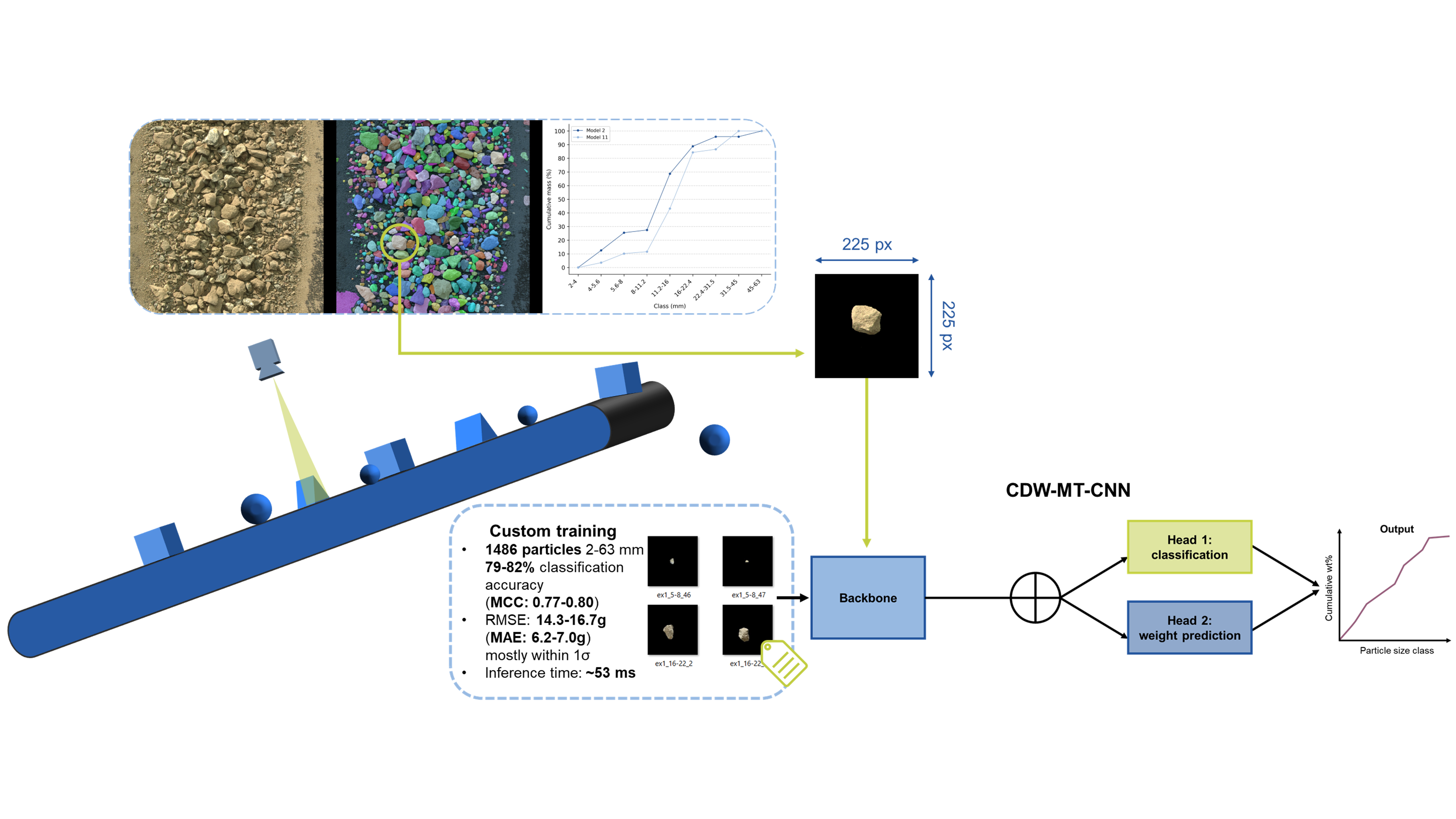
2.2.5. Quality Monitoring System
In Figure 2, the complete quality monitoring system is illustrated. Where the focus of this work is on the particle size distribution prediction part of the system, sensor recording (elaborated in Section 2.2.6) and the particle segmentation have been used as a basis for the full-scale plant experiments. For segmentation of the raw images, an adapted version of the ParticleSAM model, proposed in [43], has been implemented. This model takes high-resolution 4096 by 4096 pixel images as input, and is able to segment around 1500 particles from 4 mm or bigger (up to >63 mm) per image. As output, the adapted ParticleSAM model used in the current work provides singled-out particles in RGB format on a 225 by 225 pixel background to match the data the CDW-MT-CNN models were trained on.
The CDW-MT-CNN model then takes the segmentation model’s output as input and processes it the same way as during inference on the custom-made dataset. The classification and weight predictions results for each raw image are stored with the unique GPS label for further analysis. Optionally, the cumulative weight percentage distribution can be forwarded to the next module in the system, but this is out of scope for the current work.
2.2.6. Full-Scale Plant Experiments
In the set-up, the sensor system was constructed with all hardware elements above the fine grain conveyor of a mobile impact crusher, after which several rounds of testing and calibration were conducted. First, the stability and distance of the sensors connected to the aluminum framework were examined and adjusted until appropriate. Next, sensor-specific calibrations were conducted. This included dark signal non-uniformity (DSNU), photo response non-uniformity (PRNU) and gain calibration, as well as data transmission adjustments.
For the full-scale experiments, a set conveyor belt frequency was used, and with the help of a built-in tachometer, the speed (constancy) was verified on multiple occasions. At the same time, a custom loop circuit for theoretically endless material transportation and thus data collection and experimentation was built using a real mobile crusher conveyor belt at the standard 20 operation angle and a transportation speed of 1.5 m/s. In this process, a special focus was put on simultaneously preserving both fine and coarse fractions inside the loop, as well as minimizing the development of dust and particle breakage. This was done by adding a vibratory conveyor followed by a steep-angled return conveyor, and a slide construction — all padded with plastic flaps and covers to meet the aforementioned requirements.
Moreover, custom, python-based recording software was developed to collect all necessary data in the required formats and include all required features for the envisioned experiments and quality monitoring system in general. More specifically, for the recording software, files are always saved with the astropy GPS time stamp (when saving is turned on) to allow time-dimensional comparison and coupling with other data, such as sample (meta)data and machine data. Most of the basic features embedded in the standard delivered software remained in the custom software, such as determining the location in which the data should be saved and the option to live view the latest image. In order to allow a one-to-one comparison of the behavior of the two final CDW-MT-CNNs, it was decided to record the images live, while conducting the sampling campaigns, but to store these raw images and process them separately by the quality monitoring pipeline for each model. Each image is recorded approximately one second after the previous and given the line scanning characteristic, the complete material stream is recorded without gaps.
3. Results
3.1. Model Training
In Figure 3, the learning curves of all models in terms of accuracy (classification performance) and RMSE (weight prediction performance) are shown. Here, it can be seen that the models with identical learning rates cluster together, having similar learning durations as well as performance. In general, the models with the largest learning rate (0.001), have the worst accuracy. However, for weight prediction, this is not always the case. That is, model 3 and model 6 achieve the best RMSE for the original and stability test, respectively, compared to the other models also trained on the non-augmented data set.
The best performance averaged over the five folds for each model is shown in Table 2. The models trained on the augmented data set in general seem to classify and predict the weight with high correctness, but it should be noted that some overfitting may have occurred due to large number of augmented images present in the data set. However, even for the models not making use of the augmented data, classification accuracy ranges between 83% and 88%. Similarly, the weight prediction error is relatively constant for these models, ranging between 14.0 g and 12.5 g. Given that the mean weight of the particles in this data set ranges between 1 mg and 104 g (with an overall standard deviation of 35.6 g), this performance is considered sufficient. Based on these results, the configurations from model 2 and model 11 are used for a final retraining on the complete data set and testing on the unseen test data set. Furthermore, after a warm-up phase of 10 iterations, model 2 has a combined (i.e. both weight prediction and classification) inference time of 52.8 ms (average over five rounds of inference) per image for a 16GB NVIDIA RTX 4090 GPU. Similarly, model 11 has an inference time of 54.6 ms on GPU. For CPU, the inference times are 100.8 ms and 76.9 ms, respectively.
3.2. Performance on Unseen Data
3.2.1. Classification
To assess the classification performance in an unbiased manner, confusion matrices were analyzed, which can be found in Figure 4. In general both models are able to classify most particles correctly, acquiring an accuracy of 82% (MCC: 0.80) and 79% (MCC: 0.77) for model 2 and model 11, respectively. That both models are able to capture and process information from the 2D-RGB images for classification is furthermore indicated by the low number of particles that are classified more than one class distanced from the original class: 4 particles (or 1.3%) for model 2 (see Figure 4a) and 6 particles (or 2.0%) for model 11 (see Figure 4b). When normalizing the number of classified particles based on the true class (see Figure 4c,d), it can be seen that model 2 has an approximately equal (high) performance for particles ranging from 4 to 31.5 mm and that model 11 is more sensitive towards particles in the ranges 5.6 to 11.2 mm and 22.4 to 45 mm. Moreover, both models misclassify larger particles more often, but this behavior is more prominent for model 2, compared to model 11.
When looking at the saliency maps of four representative particles used for testing the models’ performance (see Figure 5), several things have drawn our attention. First, for small particles the pixels where the particle is located the activation intensity is high, whereas for larger — and especially the largest — particles, the area and background around the particle have high intensity but not the pixels representing the particle. Second, for model 11 more pixels have high activation intensity except for the smallest particles, which could explain the poorer performance of this model on classifying the smallest classes compared to model 2.
3.2.2. Regression
For model 2, the RMSE for the entire test set equals 14.30 g. For model 11 it equals 16.69 g. Similarly, the RMSE for nearly all (true) classes, is lower for model 11 compared to model 2, as can be seen in Table 3, with the exception of the coarse fraction, where especially the biggest class is predicted with larger error. Since model 11 was able to correctly predict all particles in the class 31.5 to 45 mm, it makes sense to analyze the RMSE for this class in more detail. For this predicted class, the RMSE equals 22.5 g (see Table 3), which is a mean difference of 29.7% compared to the mean weight. Assuming the residuals are approximately normally distributed, would mean that 95% of the observations will fall within ±45.0 g of the predicted values. It is also important to assess the error without as much influence of outliers, in particular due to the large variation in weight values for each of the classes. As such, the MAE has additionally been calculated for both models and for both groupings (i.e. true class and predicted class). The MAE equals 6.15 g for model 2 and 6.99 g for model 11. The results per group, again grouped for the true classes as well as the predicted classes, are shown in Table 4. These results show that the absolute error for the largest class is on average lower for both models compared to the RMSE values, suggesting the presence and influence of outliers. Similar patterns are also visible for the other classes. Additionally, consistent with the RMSE values, model 11 has much lower MAE values for the two lowest classes (2 to 5.6 mm) and the middle fractions (8 to 22.4 mm), where the error is up to 57% lower compared to model 2. Especially the 0.7 g (or 0.9-1.0 g when weighing outliers more heavily) absolute error on average for particles with a mean weight of 3.6 g is a promising first result that the weight of CDW particles could be predicted from 2D-RGB data.
As for most classes, both the RMSE and the MAE seem relatively high, it makes sense to compare these values to the standard deviation for each class (see Table 3). From this comparison, it becomes clear that most of the errors fall within one standard deviation from the class mean. Especially interesting are the predictions for the classes 11.2 to 16 mm, 22.4 to 31.5 mm and 45 to 63 mm, where all error values for both models fall within one standard deviation from the mean. Moreover, when looking at the MAE, besides the two smallest classes, for model 2 the predictions for two classes — namely, 8 to 11.2 mm and 16 to 22.4 mm, are on average more than one standard deviation off. This also holds for the two smallest classes for model 11, as well as particles from 31.5 to 45 mm when grouped based on the true class.
Similarly to the analysis of classification behavior, saliency maps have been analyzed for the regression part of the models. Interestingly, for model 2, no activation is visible for the smallest particle (see Figure 6a), and the activation for the medium-sized particles only spans part of the image (see Figure 6b,c). Nonetheless, here too, for both models it can be seen that the pixels representing the particles are less activated compared to the background. Additionally, for the largest particle a clear peak in activation intensity is visible around the left contour of the particle (see Figure 6d).
3.3. Performance on Full-Scale Plant Data
When comparing the predicted cumulative wt% distributions based on the models’ classifications and weight predictions with the true PSDs acquired from the sieve analyses, visualized in Figure 7, it can be seen that model 2 is able to capture the cumulative trend for the smallest classes, up until the class with particles from 8 to 11.2 mm. However, this excludes the class 2 to 4 mm, which is largely embedded in the subsequent class, due to limited training (see Section 3.2.1. Looking at the results for the larger classes, an overestimation is especially visible for the particles ranging from 11.2 to 22.4 mm, which may stem from the relatively large weight prediction error for the class 16 to 22.4 mm and the misclassifications between these two classes, as indicated in Figure 4.
Interestingly, model 11 consistently underestimates the cumulative wt% of the smallest classes — albeit following the cumulative trend — but approaches the true share for the class 11.2 to 16 mm, in particular for the second sample (see Figure 7b). Furthermore, both models obtained different results from each image, visualized by the interquartile ranges (i.e. the boxes), bounds and sometimes outliers. In this context, it should however be noted that the models merely analyze particles on the top layer of the multilayer material stream, meaning that there is likely to be some discrepancy between the PSD obtained by sieve analysis and the particles captured by the RGB sensor and segmentation procedure. Additionally, due to the practical constraints, there is no true PSD for a singular image available, but instead images within the time stamp range of the sample are aggregated for comparison.
In Figure 8, the first image and the corresponding segmentation map as well as the predicted PSDs for each of the samples is shown. This indicates which particles are included in the prediction of the PSD and what the predicted PSD of the corresponding image looks like. In the segmentation colormaps, it is clear that many of the small particles are not distinguished by the segmentation model, which — as described in Section 2.2.5 — introduces another source of uncertainty that complicates the comparison of the PSD acquired from the sieve analysis compared to the one predicted by either model. Furthermore, the examples show that even though the image illumination can change during outside operation, both the segmentation and the PSD prediction parts seem to be relatively robust to these changes.
3.4. Limitations and Future Work
Since this work focused on the development of the CDW-MT-CNN model as a novel architecture for predicting the particle size distribution and investigating its feasibility to predict a particle’s weight from 2D-RGB data while maintaining high classification performance, and at the same time take into account practical prerequisites, several starting points for further research are provided based on the remaining limitations.
First, the size of the data set in combination with the high variability of the particle weights is minimal, as is indicated by the large errors for some classes. We used a combination of data augmentation techniques to mitigate this limitation, which seems effective for most classes. However, to further optimize the predictive performance, for both classification and regression, a more extensive data set would be beneficial. Besides creating a larger data set for this particular target fraction, it would be useful to create data sets with different target fractions so that models can be trained (e.g. with transfer learning) and configured depending on the desired target fraction, which has high practical relevance.
Second, the error embedded in the prediction of the particle size distributions with the quality monitoring pipeline stems from 5 kinds of error and uncertainty, of which some are aleatoric (i.e. cannot be reduced). This regards the sieving process and extreme vibrations as well as different bulk heights slightly changing the distance from sensor to particle during operation. The other errors could be improved with further optimization of the used models, namely by improving the segmentation performance of ParticleSAM and the predictive performance — especially in terms of its weight prediction — of the proposed CDW-MT-CNN. The CDW-MT-CNN architecture can for instance be optimized by conducting an in-depth ablation study, but also by (re)training on a bigger data set. Related to this, the results of the full-scale plant examples presented in this work show the importance and difficulty of developing suitable and sound methods to validate quality monitoring systems on pilot- and full-scale plants. Currently, no verified methods exist to extract the true particle size distribution (or other material characteristics) from a batch that exactly matches one or multiple images processed by the quality monitoring system. As such, further research could focus on investigating ways of how this could be achieved.
4. Conclusions
Achieving higher transparency of the material specifications of processed CDW material is essential for boosting the use of CDW recycled aggregates in high-quality applications. One crucial specification is the particle size distribution, which is comprised of a particle classification in terms of size and the cumulative weight percentage of the particles contained in these particular classes. A major problem exists however in the translation from 2D (or 3D) data to accurate weight approximation and thus accurate PSDs. As such, in this work, we propose a novel CNN-based deep learning model, namely CDW-MT-CNN, which is able to classify the particles and their weight simultaneously based on an RGB-image in 54 ms per image. To develop this model, we manually photographed and weighed 1,486 CDW particles to develop a realistic data set and further increased the size of the training set using different augmentation techniques. Based on this data set 12 different configurations of the CDW-MT-CNN architecture have been tested on two different seeds.
The best model trained on the original data set (model 2) is able to achieve 82% accuracy with a MCC-score of 0.80 for the classification and an overall MAE of 6.15. The model trained on the augmented data has overall slightly worse performance: 79% classification accuracy and 6.99 weight prediction error. However, augmentation seems beneficial for the weight prediction of the middle fractions (i.e. 5.6 to 22.4 mm), suggesting that augmentation can be a suitable technique to mitigate data labeling limitations for CDW-related data set creation.
Results of the full-scale plant experiment further indicate lower performance for the largest particle size classes, which is also shown in the misclassifications on the labeled data set. However, model 2 in particular shows the feasibility of predicting the PSD with close approximation to the true distribution for particles ranging from 4 to 11.2 mm. Moreover, these experiments have shown the difficulty of validating a quality monitoring system on a full-scale plant due to the infeasibility of acquiring exact true distributions for each individual image and the additional uncertainties that are embedded in full-scale plants, such as severe vibrations and throughput fluctuations.
Nonetheless, this work shows that the CDW-MT-CNN architecture is able to predict the particle sizes with high correctness and the particle weight for many of those classes within one standard deviation from the mean, which provides a valuable basis for further optimization of this architecture. Furthermore, using a praxis-oriented approach, a focus was put on creating a lightweight and fast model. With average inference times of 54 ms per image, this too is a suitable basis [RQ1]. The architecture also shows to an extent decent results for the full-scale plant experiments, but further validation on the practical levels should be conducted. Furthermore, the model can be used as a part of the quality monitoring system, but for inline monitoring in a full-scale plant, the combined quality monitoring system should ideally process with a frequency of one image per second to monitor the entire stream, which is not yet achievable with the current inference time. Nonetheless, further optimization in terms of inference speed and predictive performance is expected to provide models with a performance that is able to support the manual quality assessments and therewith the improved recycling of CDW for recycled aggregates in high-quality applications [RQ2].
Author Contributions
Conceptualization, L.G., K.R. and K.G.; methodology, L.G.; software, L.G.; validation, L.G.; formal analysis, L.G.; investigation, L.G. and S.O.; resources, L.G.; data curation, L.G.; writing—original draft preparation, L.G. and S.O.; writing—review and editing, L.G. and K.R.; visualization, L.G.; supervision, K.G.; project administration, K.R.; funding acquisition, K.R. and K.G. All authors have read and agreed to the published version of the manuscript.
Funding
This work was funded by the German Federal Ministry of Education and Research (BMBF), now the German Federal Ministry of Research, Technology and Space (BMFTR), within the program "Digital GreenTech" under the project KIMBA (grant no. 2WDG1693D). Open access funding was provided by the RWTH Aachen University Open Access Publication Fund. The responsibility for the content of this publication lies with the authors.
Data Availability Statement
The datasets presented in this article are not readily available because the data are part of an ongoing study. Requests to access the datasets should be directed to the corresponding author.
Acknowledgments
The authors would like to extend their appreciation to MAV GmbH and KLEEMANN GmbH for supporting this study.
Conflicts of Interest
The authors declare no conflicts of interest.
Abbreviations
The following abbreviations are used in this manuscript:
| CDW | Construction and demolition waste |
| CDW-MT-CNN | Construction and building waste |
| multitask-convolutional neural network | |
| CEL | Cross-entropy loss |
| CMOS | Complementary metal-oxide-semiconductor |
| CNN | Convolutional neural network |
| CPU | Central processing unit |
| DSNU | Dark signal non-uniformity |
| GPS | Global positioning system |
| GPU | Graphics processing unit |
| MAE | Mean absolute error |
| MCC | Matthews correlation/Phi coefficient |
| MRI | Magnetic resonance imaging |
| PRNU | Photo response non-uniformity |
| PSD | Particle size distribution |
| RC | recycled concrete |
| ReLU | Rectified linear unit |
| RGB | Red-green-blue |
| RMSE | Root mean square error |
| TRL | Technology readiness level |
| wt% | Percentage by weight |
| 2D | Two-dimensional |
| 3D | Three-dimensional |
References
- Eurostat. Generation of waste by waste category, hazardousness and NACE Rev. 2 activity. [CrossRef]
- European Commission. EU construction sector: in transition towards a circular economy; Technical report; European Construction Sector Observatory, 2019. [Google Scholar]
- E3G. Renovate2Recover: How transformational are the National Recovery Plans for Buildings Renovation? E3G, Technical report. 2021. [Google Scholar]
- Global Property Guide News Team. Germany’s housing market remains strong.
- Bundesministerium für Wohnen; Stadtentwicklung und Bauwesen. Maßnahmenpaket der Bundesregierung.
- Statistisches Bundesamt. Bauschuttaufbereitungsanlagen: Deutschland, Jahre, Abfallarten.
- Tam, V.W.; Soomro, M.; Evangelista, A.C.J. A review of recycled aggregate in concrete applications (2000–2017). Construction and Building Materials 172, 272–292. [CrossRef]
- Choudhary, J.; Kumar, B.; Gupta, A. Utilization of solid waste materials as alternative fillers in asphalt mixes: A review. Construction and Building Materials 234, 117271. [CrossRef]
- Göbbels, L.; Feil, A.; Raulf, K.; Greiff, K. Current State of the Art and Potential for Construction and Demolition Waste Processing: A Scoping Review of Sensor-Based Quality Monitoring and Control for In- and Online Implementation in Production Processes. Sensors 25, 4401. [CrossRef] [PubMed]
- Kandlbauer, L.; Khodier, K.; Ninevski, D.; Sarc, R. Sensor-based Particle Size Determination of Shredded Mixed Commercial Waste based on two-dimensional Images. Waste Management 120, 784–794. [CrossRef]
- Di Maria, F.; Bianconi, F.; Micale, C.; Baglioni, S.; Marionni, M. Quality assessment for recycling aggregates from construction and demolition waste: An image-based approach for particle size estimation. Waste Management 48, 344–352. [CrossRef] [PubMed]
- Kroell, N.; Thor, E.; Göbbels, L.; Schönfelder, P.; Chen, X. Deep learning-based prediction of particle size distributions in construction and demolition waste recycling using convolutional neural networks on 3D laser triangulation data. Construction and Building Materials 466, 140214. [CrossRef]
- Bilodeau, M.; Gouveia, D.; Demers, A.; Di Feo, A. 3D free fall rock size sensor. Minerals Engineering 148. [CrossRef]
- Shimizu, H.; Fukuda, T.; Yabuki, N. Deep-learning Point Cloud Classification for Estimating the Weight of Single-material Construction and Demolition Waste of Unknown Shape. In Proceedings of the Proceedings of the 41st Conference on Education and Research in Computer Aided Architectural Design in Europe (eCAADe 2023), 2023; pp. 609–618. [Google Scholar] [CrossRef]
- Di Maria, A.; Eyckmans, J.; Van Acker, K. Downcycling versus recycling of construction and demolition waste: Combining LCA and LCC to support sustainable policy making. Waste Management 75, 3–21. [CrossRef]
- Einführung in die Kreislaufwirtschaft: Planung, Recht, Verfahren. In Einführung in die Kreislaufwirtschaft: Planung, Recht, Verfahren, 6. Auflage ed.; Kranert, M., Ed.; Springer Vieweg, 2024. [Google Scholar] [CrossRef]
- Göbbels, L.; Kroell, N.; Raulf, K. Towards an improvement of construction and demolition waste recycling: investigating the feasibility of using AI-based quality control using sensor-based monitoring of particle size distributions. In Global Guide of the Filtration and Separation Industry 2024-2026; Vulkan Verlag GmbH, 2025; pp. 124–130. [Google Scholar]
- Alimi, K.; Jin, R.; Nguyen, N.; Nguyen, Q.; Hosking, L. Exploring artificial intelligence applications in construction and demolition waste management: a review of existing literature. Journal of Science and Transport Technology 5, 104–136. [CrossRef]
- Hussain, R.; Alican Noyan, M.; Woyessa, G.; Retamal Marín, R.R.; Antonio Martinez, P.; Mahdi, F.M.; Finazzi, V.; Hazlehurst, T.A.; Hunter, T.N.; Coll, T.; et al. An ultra-compact particle size analyser using a CMOS image sensor and machine learning. Light: Science & Applications 9, 21. [CrossRef] [PubMed]
- Idroas, M.; Najib, S.; Ibrahim, M. Imaging particles in solid/air flows using an optical tomography system based on complementary metal oxide semiconductor area image sensors. Sensors and Actuators, B: Chemical 220, 75–80. [CrossRef]
- Kronenwett, F.; Maier, G.; Leiss, N.; Gruna, R.; Thome, V.; Längle, T. Sensor-based characterization of construction and demolition waste at high occupancy densities using synthetic training data and deep learning. Waste Management & Research: The Journal for a Sustainable Circular Economy 42, 788–796. [CrossRef]
- Beskopylny, A.N.; Shcherban’, E.M.; Stel’makh, S.A.; Razveeva, I.; Mailyan, A.L.; Elshaeva, D.; Chernil’nik, A.; Nikora, N.I.; Onore, G. Crushed Stone Grain Shapes Classification Using Convolutional Neural Networks. Buildings 1982, 15. [Google Scholar] [CrossRef]
- Deutsches Institut für Normung e.V. DIN EN 13242 Aggregates for unbound and hydraulically bound materials for use in civil engineering work and road construction.
- Deutsches Institut für Normung e.V. Tests for geometrical properties of aggregates - Part 1: Determination of particle size distribution - Sieving method.
- Deutsches Institut für Normung e.V. English version EN 13285; Unbound mixtures Specifications. 2018. [CrossRef]
- Kroell, N.; Schönfelder, P.; Chen, X.; Johnen, K.; Feil, A.; Greiff, K. Sensorbasierte Vorhersage von Korngrößenverteilungen durch Machine Learning Modelle auf Basis von 3D- Lasertriangulationsmessungen. In Proceedings of the 11. DGAW-Wissenschaftskongress "Abfall- und Ressourcenwirtschaft", 2022. [Google Scholar]
- Pacheco, J.; De Brito, J. Recycled Aggregates Produced from Construction and Demolition Waste for Structural Concrete: Constituents, Properties and Production. Materials 14, 5748. [CrossRef]
- Shorten, C.; Khoshgoftaar, T.M. A survey on Image Data Augmentation for Deep Learning. Journal of Big Data 6, 60. [CrossRef]
- Wodzinski, M.; Kwarciak, K.; Daniol, M.; Hemmerling, D. Improving deep learning-based automatic cranial defect reconstruction by heavy data augmentation: From image registration to latent diffusion models. Computers in Biology and Medicine 182, 109129. [CrossRef]
- Perez, L.; Wang, J. The Effectiveness of Data Augmentation in Image Classification using Deep Learning. [cs]. [CrossRef]
- Mumuni, A.; Mumuni, F. Data augmentation: A comprehensive survey of modern approaches. Array 16, 100258. [CrossRef]
- Islam, T.; Hafiz, M.S.; Jim, J.R.; Kabir, M.M.; Mridha, M. A systematic review of deep learning data augmentation in medical imaging: Recent advances and future research directions. Healthcare Analytics 5, 100340. [CrossRef]
- Howard, A.; Sandler, M.; Chu, G.; Chen, L.C.; Chen, B.; Tan, M.; Wang, W.; Zhu, Y.; Pang, R.; Vasudevan, V.; et al. Searching for MobileNetV3. [cs]. [CrossRef]
- Krizhevsky, A.; Sutskever, I.; Hinton, G.E. ImageNet classification with deep convolutional neural networks. Commun. ACM 60, 84–90. [CrossRef]
- Wang, H.; Raj, B. On the Origin of Deep Learning, [1702.07800 [cs]]. version: 4. [CrossRef]
- Simonyan, K.; Zisserman, A. Very Deep Convolutional Networks for Large-Scale Image Recognition. 1409.1556 [cs]. [CrossRef]
- Szegedy; Liu, C.; Wei; Jia, Yangqing; Sermanet, P.; Reed, S.; Anguelov, D.; Erhan, D.; Vanhoucke, V.; Rabinovich, A. Going deeper with convolutions. In Proceedings of the 2015 IEEE Conference on Computer Vision and Pattern Recognition (CVPR); IEEE, 2015; pp. 1–9. [Google Scholar] [CrossRef]
- Chhapariya, K.; Benoit, A.; Buddhiraju, K.M.; Kumar, A. A Multitask Deep Learning Model for Classification and Regression of Hyperspectral Images: Application to the large-scale dataset. [cs]. [CrossRef]
- Padmapriya, K.; Periyathambi, E. Joint classification and regression with deep multi task learning model using conventional based patch extraction for brain disease diagnosis. PeerJ Computer Science 10, e2538. [CrossRef]
- Wilson, A.C.; Roelofs, R.; Stern, M.; Srebro, N.; Recht, B. The Marginal Value of Adaptive Gradient Methods in Machine Learning. In Proceedings of the Advances in Neural Information Processing Systems, 2017; Curran Associates, Inc.; Vol. 30. [Google Scholar]
- Stoica, P.; Babu, P. Pearson–Matthews correlation coefficients for binary and multinary classification. Signal Processing 222, 109511. [CrossRef]
- Branco, P.; Torgo, L.; Ribeiro, R. A Survey of Predictive Modelling under Imbalanced Distributions. Version Number 2. [CrossRef]
- Zhou, Y.; Thielmann, P.; Chamoli, A.; Mirbach, B.; Stricker, D.; Raphael Rambach, J. ParticleSAM: Small Particle Segmentation for Material Quality Monitoring in Recycling Processes. Proceedings of the Proceedings of the 33rd European Signal Processing Conference (EUSIPCO 2025) IEEE 2025, Vol. 33, p. tbd. [Google Scholar]
Figure 1.
(a) Raw, non-comminuted input material. (b) Material after comminution and sieve analysis.
Figure 1.
(a) Raw, non-comminuted input material. (b) Material after comminution and sieve analysis.

Figure 2.
Graphical representation of the used quality monitoring system.

Figure 3.
Learning curve for each of the models in terms of accuracy (classification) and RMSE (weight prediction). Abbreviations: lr = learning rate; = weight coefficient of the regression loss. (a) Accuracy learning curves of the models trained on the original data using the original seed (left) and the seed used for stability testing (right). (b) Accuracy learning curves of the models trained on the augmented data using the original seed (left) and the seed used for stability testing (right). (c) RMSE learning curves of the models trained on the original data using the original seed (left) and the seed used for stability testing (right). (d) RMSE learning curves of the models trained on the augmented data using the original seed (left) and the seed used for stability testing (right).

Figure 4.
Confusion matrices to visualize the classification performance for the final models (a) Confusion matrix with the number of correctly (diagonal) and falsely (non-diagonal) predicted particles for model 2. (b) Confusion matrix with the number of correctly (diagonal) and falsely (non-diagonal) predicted particles for model 11. (c) Confusion matrix with the percentage of correctly (diagonal) and falsely (non-diagonal) predicted particles for model 2, normalized based on the true class. (d) Confusion matrix with the percentage of correctly (diagonal) and falsely (non-diagonal) predicted particles for model 11, normalized based on the true class.

Figure 5.
Saliency maps for the classification head. For each subfigure, from left to right: 1) input image; 2) saliency map model 2; 3) overlay saliency map and input image model 2; 4) saliency map model 11; and 5) overlay saliency map and input image model 11 (a) Particle from class 4-5.6 mm (correctly predicted by either model). (b) Particle from class 11.2-16 mm (falsely predicted by either model (16-22.4 mm)). (c) Particle from class 16-22.4 mm (falsely predicted by model 2 (11.2-16 mm)). (d) Particle from class 45-63 mm (correctly predicted by either model) and color map of the activation intensity for all subfigures

Figure 6.
Saliency maps for the regression head. For each subfigure, from left to right: 1) input image; 2) saliency map model 2; 3) overlay saliency map and input image model 2; 4) saliency map model 11; and 5) overlay saliency map and input image model 11 (a) Particle with g (model 2: 0.43 g; model 11: 0.07 g). (b) Particle with g (model 2: 4.92 g; model 11: 7.31 g). (c) Particle with g (model 2: 3.84 g; model 11: 3.36 g). (d) Particle with g (model 2: 117.49 g; model 11: 161.61 g) and color map of the activation intensity for all subfigures.

Figure 7.
Comparison of the true PSDs with the predicted values for both models. (a) The first sample taken for validation. (b) The second sample taken for validation.
Figure 7.
Comparison of the true PSDs with the predicted values for both models. (a) The first sample taken for validation. (b) The second sample taken for validation.

Figure 8.
Examples of raw images (left), the segmentation process in the form of color maps highlighting the segmented particles (middle) and the predicted cumulative wt% distribution (right). (a) The first recorded image from sample 1. (b) The first recorded image from sample 2.
Figure 8.
Examples of raw images (left), the segmentation process in the form of color maps highlighting the segmented particles (middle) and the predicted cumulative wt% distribution (right). (a) The first recorded image from sample 1. (b) The first recorded image from sample 2.


Table 1.
Number of particles recorded and used in the dataset for each class.
| Class (mm) |
Nr. particles (-) |
Particle weight (g) |
| 2-4 | 16 | 0.051 ± 0.033 |
| 4-5.6 | 260 | 0.118 ± 0.045 |
| 5.6-8 | 200 | 0.428 ± 0.219 |
| 8-11.2 | 199 | 1.197 ± 0.455 |
| 11.2-16 | 200 | 3.256 ± 1.437 |
| 16-22.4 | 200 | 8.368 ± 3.808 |
| 22.4-31.5 | 157 | 28.468 ± 15.919 |
| 31.5-45 | 103 | 73.059 ± 24.618 |
| 45-63 | 151 | 98.875 ± 42.300 |
Table 2.
Average validation accuracy, MCC and RMSE over 5 folds for each model. Bold values indicate the overall best value for the original seed, bold and italicized values indicate the overall best value for the stability tests, and italicized values indicate the highest performance for the original seed and stability tests for the models trained on the original data (model 1-6). Model 7-12 regard the augmented data. For accuracy and MCC: the higher the value, the better the performance. For RMSE: the lower the value, the better the performance.
| Accuracy | MCC | RMSE | |
| Model | |||
| Model 1 | 0.882 | 0.866 | 13.706 |
| Model 1 (s) | 0.857 | 0.836 | 13.420 |
| Model 2 | 0.876 | 0.858 | 13.317 |
| Model 2(s) | 0.857 | 0.837 | 12.580 |
| Model 3 | 0.838 | 0.815 | 13.233 |
| Model 3 (s) | 0.838 | 0.815 | 13.182 |
| Model 4 | 0.872 | 0.853 | 13.922 |
| Model 4 (s) | 0.840 | 0.817 | 13.498 |
| Model 5 | 0.856 | 0.835 | 14.031 |
| Model 5 (s) | 0.849 | 0.828 | 12.614 |
| Model 6 | 0.842 | 0.819 | 12.499 |
| Model 6 (s) | 0.834 | 0.811 | 12.502 |
| Model 7 | 0.970 | 0.965 | 5.408 |
| Model 7 (s) | 0.976 | 0.972 | 5.839 |
| Model 8 | 0.985 | 0.983 | 4.040 |
| Model 8 (s) | 0.987 | 0.985 | 4.681 |
| Model 9 | 0.964 | 0.959 | 4.538 |
| Model 9 (s) | 0.961 | 0.955 | 5.680 |
| Model 10 | 0.958 | 0.952 | 4.814 |
| Model 10 (s) | 0.961 | 0.955 | 5.352 |
| Model 11 | 0.981 | 0.978 | 3.983 |
| Model 11 (s) | 0.985 | 0.982 | 3.881 |
| Model 12 | 0.950 | 0.943 | 4.712 |
| Model 12 (s) | 0.948 | 0.941 | 5.124 |
Table 3.
RMSE’s of the final models per class, where (true class) refers to a grouping based on the true labels and (predicted class) on the predicted labels, respectively.
Table 3.
RMSE’s of the final models per class, where (true class) refers to a grouping based on the true labels and (predicted class) on the predicted labels, respectively.
| Class (mm) |
Mean weight (g) |
RMSE model 2 (true class) |
RMSE model 2 (predicted class) |
RMSE model 11 (true class) |
RMSE model 11 (predicted class) |
| 2-4 | 0.04 ± 0.03 | 0.382 | - | 0.171 | - |
| 4-5.6 | 0.11 ± 0.05 | 0.316 | 0.322 | 0.118 | 0.125 |
| 5.6-8 | 0.44 ± 0.22 | 0.201 | 0.245 | 0.198 | 0.230 |
| 8-11.2 | 1.17 ± 0.48 | 0.655 | 0.634 | 0.540 | 0.462 |
| 11.2-16 | 3.58 ± 1.75 | 1.287 | 1.537 | 1.020 | 0.905 |
| 16-22.4 | 8.47 ± 3.78 | 6.214 | 6.153 | 2.810 | 2.664 |
| 22.4-31.5 | 26.11 ± 19.67 | 10.615 | 11.377 | 13.208 | 13.444 |
| 31.5-45 | 75.66 ± 23.26 | 28.071 | 25.487 | 43.318 | 22.511 |
| 45-63 | 104.25 ± 50.78 | 35.710 | 35.743 | 35.108 | 39.840 |
Table 4.
Mean absolute errors of the final models per class, where (true class) refers to a grouping based on the true labels and (predicted class) on the predicted labels, respectively.
Table 4.
Mean absolute errors of the final models per class, where (true class) refers to a grouping based on the true labels and (predicted class) on the predicted labels, respectively.
| Class (mm) |
MAE model 2 (true class) |
MAE model 2 (predicted class) |
MAE model 11 (true class) |
MAE model 11 (predicted class) |
| 2-4 | 0.381 | - | 0.170 | - |
| 4-5.6 | 0.312 | 0.317 | 0.094 | 0.099 |
| 5.6-8 | 0.143 | 0.173 | 0.159 | 0.188 |
| 8-11.2 | 0.518 | 0.491 | 0.374 | 0.332 |
| 11.2-16 | 1.026 | 1.146 | 0.797 | 0.714 |
| 16-22.4 | 4.724 | 4.614 | 2.194 | 1.999 |
| 22.4-31.5 | 7.358 | 8.007 | 8.867 | 8.843 |
| 31.5-45 | 22.439 | 21.381 | 37.308 | 20.288 |
| 45-63 | 27.864 | 28.446 | 28.450 | 33.546 |
Disclaimer/Publisher’s Note: The statements, opinions and data contained in all publications are solely those of the individual author(s) and contributor(s) and not of MDPI and/or the editor(s). MDPI and/or the editor(s) disclaim responsibility for any injury to people or property resulting from any ideas, methods, instructions or products referred to in the content. |
© 2026 by the authors. Licensee MDPI, Basel, Switzerland. This article is an open access article distributed under the terms and conditions of the Creative Commons Attribution (CC BY) license (http://creativecommons.org/licenses/by/4.0/).
Copyright: This open access article is published under a Creative Commons CC BY 4.0 license, which permit the free download, distribution, and reuse, provided that the author and preprint are cited in any reuse.


