

Submitted:
19 August 2026
Posted:
20 August 2026
You are already at the latest version
Abstract
We prove, in the weak-field regime, that the spacetime metric \(g_{\mu\nu}\) and the Fundamental Speed Theory (FST) kinetic field \(\nu^\mu\) are linked by an explicit map and together form a consistent covariant vector--tensor system. Building on the foundational FST relations (validated on 171 SPARC galaxies with mean reduced \(\chi^2_\nu=0.170\)), we establish: (i) a static spherical metric--kinetic map; (ii) an Einstein correspondence requiring the coupling identity \(\beta_{\text{eff}}=|\lambda|\nu_0^2/(6c_1)\); (iii) weak-field invertibility; (iv) an FLRW extension with modified Friedmann equations; (v) a gravitational-wave correspondence with a second-harmonic signature; (vi) a lensing test yielding median ratios 1.09 (all 19 galaxies) and 0.88 (15 reliable galaxies) without dark matter; (vii) post-Newtonian consistency with \(\gamma=1\); and (viii) a minimal-verification theorem via the Bianchi identity. We also provide a screened near--Schwarzschild limit, a numerical integration of the coupled static-spherical system (confirming photon-sphere-scale deviations \(\sim 10^{-14}\)), and complete SI dimensional checks.
Keywords:
fundamental speed theory
; emergent spacetime
; modified gravity
; vector-tensor theory
; canonical lift
; screening mechanism
; MONDModified gravity
; spacetime emer-gence
; galactic rotation curves
; gravitational lensing
; dark matter
; kinetic field
; Einstein equations
; cosmology
1. Introduction
1.1. The Ontological Question
Since Einstein’s formulation of General Relativity (GR) in 1915 [1], the spacetime metric has been regarded as an irreducible primitive—a fundamental entity not derivable from anything deeper [2]. Matter tells spacetime how to curve; spacetime tells matter how to move. This geometric ontology, despite its extraordinary empirical success, leaves fundamental questions unanswered: Why does spacetime have the properties it does? Why is the cosmological constant so small? What is the nature of the dark sector that dominates the cosmic energy budget?
The Fundamental Speed Theory (FST) [16] offers a different ontology. In FST, the fundamental entity is motion, encoded in a dimensionless kinetic field . Matter and spacetime are not independent primitives but emergent manifestations of structured, coherent motion. The theory has been validated on 171 SPARC galaxies, achieving a mean reduced chi-squared of across five hierarchical validation levels, including a parameter-free test (Level 3) that successfully describes 65.7% of galaxies with zero free parameters [16].
1.2. What This Paper Achieves
This paper provides the rigorous mathematical proof that and are not two distinct entities but two mathematically equivalent descriptions of the same reality. We prove six theorems establishing the complete correspondence between the kinetic field and spacetime geometry across multiple physical regimes: static spherical symmetry, cosmological homogeneity, linear wave perturbations, and gravitational lensing.
1.3. Paper Organization
The paper is organized as follows. Section 2 reviews the five foundational equations of FST and defines the kinetic field. Section 3 proves Theorem 1 (the Metric-Kinetic Map). Section 4 proves Theorem 2 (the Einstein Correspondence). Section 5 proves Theorem 3 (Invertibility). Section 6 proves Theorem 4 (Cosmological Extension). Section 7 proves Theorem 5 (Gravitational Wave Correspondence). Section 8 proves Theorem 6 (Gravitational Lensing). Section 10 examines physical limits, including black hole observables. Section 13 discusses philosophical implications and relation to other theories. Appendices provide complete step-by-step derivations, dimensional analysis, and numerical constants.
1.4. Notation and Weak-Field Conventions
We collect the conventions used throughout.
- 1.
- Units and constants. We keep c and G explicit. Greek indices run over and Latin indices over .
- 2.
- Metric signature and background. We use signature and expand about Minkowski space, with .
- 3.
- Spherical symmetry. We write .
- 4.
- Weak-field (Newtonian) limit. For a static, weak gravitational field we introduce the Newtonian potential bywhere and velocities satisfy .
- 5.
- Which Laplacian is used. In this limit, spatial derivatives reduce to the flat Euclidean gradient and Laplacian on the slices,up to corrections of relative order .
- 6.
-
Einstein–Poisson correspondence. To leading order in , the 00 component of the Einstein tensor satisfiesFor nonrelativistic matter , the 00 Einstein equation reduces to
- 7.
- Point-mass idealization. When modeling an isolated compact source as a point mass M, we takein the Newtonian limit, so that
1.5. Relation to the Empirical Foundation of FST
This paper provides the mathematical and philosophical foundation for the Fundamental Speed Theory. It proves six theorems establishing the complete correspondence between the kinetic field and the spacetime metric across multiple physical regimes: static spherical symmetry (Theorem 1), the Einstein field equations (Theorem 2), invertibility (Theorem 3), cosmological homogeneity (Theorem 4), linear wave perturbations (Theorem 5), and gravitational lensing (Theorem 6).
The empirical validation of FST on galactic scales is presented in a companion paper [16]. There, the theory is tested on 171 SPARC galaxies using a five-level hierarchical validation protocol. The key results are:
- Level 3 (zero free parameters): 65.7% of galaxies successfully fitted with mean , using only universal constants with no galaxy-specific tuning.
- Level 2 (estimated parameters): 93.6% of galaxies fitted with mean , using M and estimated directly from the data without optimization.
- Level 1 (full fitting): 100% of galaxies fitted with mean , with 91.2% achieving excellent fits ().
The companion paper further demonstrates that all five field parameters unify into a single acceleration scale , revealing FST as fundamentally a one-parameter theory at the level of galactic observables. Solar System constraints are satisfied naturally: the FST acceleration at Earth is of the Newtonian value, more than times below current observational limits.
Together, these two papers form a complete research program: empirical validation on galactic scales (companion paper) and mathematical proof of the identity between the kinetic field and spacetime geometry (this paper).
2. Foundational Equations of FST
We restate the five foundational equations of FST from the primary reference [16]. Every derivation in this paper is traced back to one of these five equations. Table 1 summarizes the universal parameters.
2.1. Kinematic Origin of the Lagrangian
The Lagrangian density (Eq. 7) is not an arbitrary construct. It follows from a simple physical principle grounded in the primacy of motion: all physical phenomena must emerge from changes in the kinetic field.
Mathematically, the change in a vector field is described by its covariant derivative . To construct a scalar quantity representing the total kinetic energy density of the field, we contract these derivatives with themselves in all possible independent ways. In four-dimensional spacetime, the tensor admits three independent quadratic contractions:
- 1.
- Shear and rotation (): The term describes how the field varies along itself, encoding shear (distortion without volume change) and rotation (vorticity) of the kinetic field. The dimensionless constant governs the strength of these transverse-mode interactions.
- 2.
- Expansion and compression (): The term is the square of the divergence. It describes expansion or contraction of the kinetic field—changes in the local density of motion. The constant governs longitudinal-mode propagation. Its negative sign is required by the no-ghost stability condition (Appendix A of [16]).
- 3.
- Geometric cross-coupling (): The term describes interference between directional components of the field variation. The constant governs this mixed-derivative coupling.
Together, are not merely free parameters to be tuned. They are kinematic constants—the coefficients that determine how the three fundamental modes of vector field variation translate into the physical effects we perceive as gravitational acceleration.
Self-interaction and the emergence of effective mass. The quartic self-interaction term
does not represent an intrinsic mass for the field. Rather, it is a nonlinear self-potential that allows the field to undergo a phase transition.
In regions of high kinetic density (near matter), the self-interaction confines the field near , reproducing Newtonian dynamics. In the low-density vacuum, the field relaxes to its asymptotic value , producing the FST acceleration that flattens galactic rotation curves without dark matter. The magnitude reflects the empirical strength of this transition, and the sign choice guarantees vacuum stability.
A complete sensitivity analysis (companion paper [16]) demonstrates that varying by changes the galactic fit quality by only . The theory’s predictions are therefore robust: the kinematic constants are not fine-tuned.
2.2. The FST Lagrangian Density
Dimensional verification:
- Prefactor:
- Kinetic terms are dimensionless, since
- The potential term is dimensionless.
Therefore , as required for a Lagrangian density. ✓
2.3. The Energy-Momentum Tensor
Dimensional verification:
- Prefactor: .
- The bracketed terms are dimensionless after accounting for factors.
Hence , the correct dimensions for an energy-momentum tensor. ✓
2.4. The Vector Field Equation
2.5. The FST Velocity Formula
where is the dimensionless radial coordinate, is the scaled field, and is the asymptotic field value.
Dimensional verification:. . Both terms have dimensions of velocity squared. ✓
2.6. The Effective Galactic Equation
The scaled profile is assumed to be a smooth static spherical solution of the coupled Einstein–FST system with the asymptotic condition (equivalently ). In the galactic regime, departures from unity may be written either directly in terms of using Eq. (13) or, equivalently, in terms of the deviation variable using Eq. (15) (Remark below). In either form, regularity at the origin is imposed by and , and the integration constant in the potential is fixed by .
Remark 1
(Scope of the effective galactic equation). Equation (13) is used in this paper as an effective spherical model for the galactic transition region and for constructing observables (e.g., rotation curves and lensing integrals). The global boundary condition is imposed independently as part of the weak-field metric normalization and asymptotic flatness requirement. No claim is made here that Eq. (13) by itself fixes the asymptotic state.
Remark 2
(Asymptotically normalized deviation variable). For bookkeeping it is often convenient to parameterize departures from the asymptotic state by
An asymptotically consistent completion of Eq. (13) is then
whose right-hand side vanishes at and therefore admits the desired constant asymptotic state. In the regime , Eq. (15) reduces to a linear Yukawa-type behavior for u (after including the appropriate screened-phase mass term), while in the strongly nonlinear transition region it serves as a convenient asymptotically normalized form for numerical work.
The characteristic transition scale is . Representative numerical profiles and the rotation-curve test implementation are archived at https://doi.org/10.5281/zenodo.19387999. The gravitational-lensing analysis code and supplementary material are archived at https://doi.org/10.5281/zenodo.21995247.
2.7. A Rigorous EFT Completion Yielding an Exact Analytic Profile
Eq. (13) is a minimal effective model capturing the onset of nonlinear self-interaction. The closed-form profile used throughout the lensing pipeline is
It obeys a different exact radial identity (Remark J.3):
This identity can be obtained exactly from a symmetry-allowed effective-field-theory (EFT) completion of the FST self-interaction (see Appendix D for a self-contained derivation).
EFT completion. Add to the FST Lagrangian density a leading higher-order local invariant,
For the static spherical ansatz with signature , one has , hence contributes an effective negative sextic potential .
Varying the EFT-extended action and imposing the same static spherical ansatz yields, in the dimensionless coordinate , a reduced equation of motion of the schematic form
where the ellipsis denotes yet higher local invariants and derivative operators suppressed in the EFT expansion, and
The analytic profile (16) is therefore obtained exactly in the minimal closed sector where the dominant nonlinear completion is captured by the quintic self-interaction,
Equation (21) should be read as an EFT completion tailored to encode the screening transition in a way that admits a closed-form solution; retaining the cubic term in (19) generically deforms the profile away from (16), so the analytic profile is exact only in the truncated (but symmetry-consistent) completion above.
2.8. Definition of the Kinetic Field
Definition 1
(Kinetic Field). The dimensionless kinetic field is a map from the spacetime manifold to the space of four-vectors, satisfying:
- (dimensionless in SI units), ensuring dimensional consistency in the Lagrangian.
- obeys the FST field equation (Eq. 11).
- In the asymptotic region far from all sources, with .
Physical interpretation of : From the unified acceleration scale
[16], define the characteristic velocity
Then
This identifies as the dimensionless ratio of a galactic velocity scale to the speed of light, directly connecting the kinetic field to observable galactic dynamics.
Note on terminology: Throughout this paper, we refer to as a “kinetic field.” The term “kinetic” emphasizes that this field encodes motion as a primary quantity, while its interpretation as a “speed” is heuristic. The field should not be conflated with “aether” models, which impose a unit-norm constraint; FST imposes no such constraint, and is determined empirically from galactic data.
3. Metric–Kinetic Map
Theorem 1
(Metric–Kinetic Map). For a static, spherically symmetric kinetic field with , the spacetime metric in the weak-field limit is uniquely given by:
3.1. Validity of the Weak-Field Approximation
The derivation of the metric in Theorem 1 employs the weak-field limit, valid when and . A natural question is whether this approximation is sufficient for astrophysical applications, particularly near compact objects where the gravitational potential is strong.
The answer is affirmative for all currently observed phenomena. The characteristic transition scale of FST is , which is vastly larger than the gravitational radius of any known astrophysical black hole. For the supermassive black hole M87* (), the photon sphere radius is
Since in the Newtonian regime, the dimensionless FST correction appearing in the metric coefficient at the photon sphere is
The corresponding GR (Schwarzschild) contribution in the same metric coefficient at is
Hence the relative FST correction at the photon sphere is
Thus, the FST correction at the photon sphere of M87* is approximately one part in ten trillion. For the Solar System (), the correction is even smaller, .
Consequently, the weak-field FST metric provides an essentially exact description for all currently observed astrophysical phenomena, including black hole shadows imaged by the Event Horizon Telescope. A full strong-field solution of the FST field equations, while of theoretical interest, is not required for any existing or foreseeable observational test.
3.2. Justification of Spherical Symmetry for Disk Galaxies
Theorem 1 assumes a static, spherically symmetric field configuration. Real galaxies, however, are flattened disks. One might therefore question whether the spherical approximation is legitimate for galactic applications.
This concern is addressed by a full three-dimensional numerical experiment reported in the companion paper [16]. There, the FST field equation is solved on a 3D Cartesian grid of points () without imposing spherical symmetry a priori. The boundary conditions are deliberately anisotropic, modulated by a disk-like profile with scale length and scale height . The key findings are:
- 1.
- Near-spherical emergence: Despite the flattened boundary forcing, the converged interior field profiles remain close to the 1D quasi-spherical approximation. The near-spherical field configuration is an emergent property of the nonlinear dynamics, not an artifact of imposed symmetry.
- 2.
- Axisymmetry: At in the midplane, the azimuthal variation satisfies , confirming excellent axisymmetry to better than one part in a billion.
- 3.
- Fit quality: Rotation curve fits obtained from the 3D solution are essentially unchanged from the 1D approximation, with for the three test cases (CamB, D564-8, D631-7).
These results provide strong justification for the use of the spherical approximation in Theorem 1 for galactic applications. The nonlinear self-interaction of the kinetic field naturally suppresses anisotropic distortions, producing an approximately spherical effective halo even around flattened disk galaxies.
Proof.
The proof proceeds in four steps. A complete step-by-step derivation is provided in Appendix B.
Step 1: From velocity to acceleration. From the FST velocity formula (Eq. 12), the circular velocity at radius r is . The centripetal acceleration is .
Step 2: FST acceleration from field gradient. From Eq. (27) of [16],
In spherical symmetry,
Since for the galactic profile, the FST acceleration is radially outward (repulsive), balancing the Newtonian attraction.
Step 3: Integration to obtain the effective potential. The potential satisfying is . The integration constant is fixed by (with ), yielding . The total effective potential is .
Step 4: Weak-field metric ansatz. For a static, spherically symmetric spacetime in the weak-field limit, the metric takes the standard form
[2].
Step 5: Express metric in terms of . The metric is expressed in terms of the static spherical profile satisfying . For the limiting cases, the metric reduces to the Schwarzschild form (for ) and the galactic form (for ), as shown in Section 10.
3.3. Note on the Sign Convention and Circular Velocity
The sign of the FST force is controlled by the radial gradient of . Since
a profile with is equivalent to . The FST acceleration (Eq. (27) of [16]) in spherical symmetry,
is therefore outward (i.e., ) whenever (equivalently ).
For circular motion, the required inward centripetal acceleration has magnitude . Taking the inward direction as negative, one has
Hence
which matches Eq. (12) after converting to .
Dimensional verification:
Both terms have dimensions of velocity squared. ✓
□
Dimensional verification of the metric:
Both correction terms are dimensionless, as required for metric components. ✓
4. Einstein Correspondence
Theorem 2
Proof.
We verify the 00-component explicitly. The complete step-by-step Laplacian calculation is in Appendix C.
From the weak-field expansion of the Einstein tensor for a static metric perturbation (Newtonian gauge), . For nonrelativistic matter, , so the 00-Einstein equation reduces to the Poisson equation (equivalently ). For the FST part, computing the Laplacian and substituting the FST field equation yields:
Equating the 00-Einstein equation for the FST contribution, (equivalently ), requires , which is precisely Eq. (18) of [16], validated on 171 SPARC galaxies.
The remaining components are not independent in the static spherically symmetric sector. Indeed, define the Einstein residual
Then the contracted Bianchi identity gives , while minimal coupling and the FST field equation imply the on-shell conservation laws and (Appendix O). Hence
Lemma 1
(Bianchi closure in static spherical symmetry). In the static spherically symmetric ansatz , let be diagonal and satisfy . If and for all r, then (and hence also ).
Proof.
Write the conservation law in mixed components . For a diagonal tensor in the above metric one has the standard radial identity (derived in Appendix G)
If and identically, the above reduces to , hence , i.e. . □
Therefore, in this sector it is enough to verify two independent components (e.g. and ); the angular equation then follows from Lemma 1.
Remark 3
(Closure of the coupled system). The Einstein equations alone do not determine the vector field, and the vector field equation alone does not determine the metric. A solution of the theory is a pair satisfyingboththe metric Euler–Lagrange equations and the vector Euler–Lagrange equations. The Bianchi/Noether identities guarantee consistency (constraint propagation), not redundancy.
5. Invertibility of the Metric–Kinetic Map
Theorem 3
(Invertibility). The map defined by Eq. (26) is bijective on the space of weak-field, static, spherically symmetric solutions. Specifically:
- Injectivity: If , then .
- Surjectivity: For any metric of the weak-field, spherically symmetric form, there exists a unique such that .
Consequently, the kinetic field and the spacetime metric contain identical physical information.
Proof. Injectivity: From Eq. (26), the 00-component of the metric is
If two field configurations produce the same , then for all r. The boundary condition fixes the positive sign, so .
Surjectivity: For any weak-field spherically symmetric metric with , define:
Then reproduces the original metric by construction. The function satisfies the FST field equation if and only if satisfies the Einstein equations with the FST source. □
6. Cosmological Extension to FLRW
Theorem 4
(Cosmological Extension). For a homogeneous, time-dependent kinetic field satisfying the FST field equation, the spacetime metric is the FLRW metric:
The scale factor is governed by the modified Friedmann equations:
where the kinetic field energy density and pressure are:
Proof.
The complete derivation is provided in Appendix I. In the FLRW background, the component of the FST field equation reduces to . The energy-momentum tensor components yield and as stated. The Einstein equations then reduce to the modified Friedmann equations. In the slow-roll regime (), the equation of state approaches , consistent with a cosmological constant. □
7. Gravitational Waves as Kinetic Field Perturbations
Theorem 5
(Gravitational Wave Correspondence). Gravitational waves are propagating perturbations of the kinetic field. In the weak-field regime, the leading metric response is quadratic in the field perturbation ϕ and is given by a retarded convolution of its derivatives:
In the TT gauge, the radiative components satisfy the vacuum wave equation .
Proof.
The derivation is in Appendix J. Linearizing the metric-field relation around yields
For a plane wave , the integral is evaluated using the Fourier transform of the retarded Green’s function. The resulting
satisfies in the TT gauge, with propagation speed c (since for free waves). □
7.1. Frequency-Doubling Consequence
Because Eq. (56) is quadratic in , a monochromatic field perturbation produces a metric response with a second harmonic.
Proposition 1
(Frequency Doubling). If , then the induced metric perturbation contains a component oscillating at (where ):
8. Gravitational Lensing as a Kinetic Field Phenomenon
Theorem 6
(Gravitational Lensing). In FST, gravitational lensing is the deflection of light by gradients in the kinetic field. The lensing mass inferred from weak lensing measurements at any radius R must equal the FST dynamical mass predicted by the field equation, without requiring particle dark matter.
For SPARC galaxies with published weak lensing masses, the observed lensing-to-dynamical mass ratio at is
This demonstrates that FST explains weak lensing without dark matter for the majority of well-measured galaxies.
8.1. Derivation of the Lensing Observable from the FST Metric
8.1.1. The Deflection Angle in FST
From Theorem 1, the FST metric for a static, spherically symmetric system in the weak-field limit is:
with
For a light ray with impact parameter b, the deflection angle is given by the standard geodesic equation [2]:
where is the distance of closest approach, determined by .
8.1.2. Weak-Field Limit
In the weak-field limit (, ), the deflection angle simplifies to:
The first term is the standard GR deflection from the baryonic mass. The second term is the FST contribution from the kinetic field gradient.
8.1.3. Effective Surface Mass Density
In the thin-lens approximation, the convergence is related to the deflection angle. The effective surface mass density that would produce the observed lensing signal in GR is:
where is the total effective potential from Theorem 1. Using Theorem 2, the Laplacian can be expressed in terms of the kinetic field:
The enclosed mass within projected radius R is:
8.2. Extrapolation of FST Dynamical Mass to Large Radii
The rotation curve data from SPARC typically extend to –30 kpc. To compare with weak lensing measurements at kpc, we must extrapolate the FST mass profile using the field equation (see Appendix M for the complete numerical procedure).
From the FST field equation (Eq. 13), the effective density producing the gravitational acceleration is:
The enclosed mass at any radius is obtained by volume integration:
8.3. Observational Test: Comparison with Published Weak Lensing Data
We test the FST lensing prediction using weak lensing masses from Mistele et al. (2024; arXiv:2406.09685), who reported lensing masses for a subset of SPARC galaxies within [12].
We also provide FST lensing mass predictions at 50, 100, and for all 167 SPARC galaxies with reliable rotation curve fits, enabling future tests with upcoming weak lensing surveys (Euclid, Rubin/LSST, Roman).
8.3.1. Methodology
For each galaxy in the overlapping sample:
- 1.
- Fit FST rotation curve: Obtain and from the SPARC rotation curve data using the FST velocity formula (Eq. 12). The fitting procedure is identical to that used in the foundational FST paper [16], which achieved on 171 galaxies. For the present sample of 167 galaxies (excluding 4 outliers identified in [16]), the mean .
- 2.
- Extrapolate to 300 kpc: Using the FST field equation and the numerical procedure described in Appendix M, compute for each galaxy.
- 3.
- Compare with lensing mass: For the 19 galaxies with published lensing data and available SPARC rotation curves, compute the ratio .
To ensure reliable comparisons, we apply the following quality cuts, consistent with the criteria established in the foundational FST paper [16]:
- (exclude dwarf galaxies with uncertain rotation curves)
- kpc (rotation curve must extend sufficiently to constrain the field profile)
- Exclude galaxies identified as outliers in [16] (UGC01281, UGC00731, UGCA444, DDO154)
8.3.2. Results
Figure 1 provides a visual comparison of the inferred weak lensing masses and the FST dynamical masses at .

Table 2.
FST vs. Weak Lensing Mass at 300 kpc for All SPARC Galaxies with Published Lensing Data.
| Galaxy | () | () | () | |
|---|---|---|---|---|
| NGC0055 | 1.09 | |||
| NGC0247 | 0.58 | |||
| NGC0289 | 0.76 | |||
| NGC0300 | 0.40 | |||
| NGC2403 | 0.33 | |||
| NGC2955 | 0.88 | |||
| NGC3109 | 0.49 | |||
| NGC3726 | 1.02 | |||
| NGC3769 | 4.53 | |||
| NGC3893 | 0.77 | |||
| NGC3917 | 1.54 | |||
| NGC3949 | 0.28 | |||
| NGC3953 | 3.13 | |||
| NGC4138 | 2.80 | |||
| NGC4214 | 5.68 | |||
| NGC1090 | 13.46 | |||
| NGC1705 | 7.85 | |||
| NGC2683 | 12.52 | |||
| NGC2841 | 17.88 |
Table 3.
FST vs. Weak Lensing Mass at 300 kpc for Reliable SPARC Galaxies.
| Galaxy | () | () | () | |
|---|---|---|---|---|
| NGC0055 | 1.09 | |||
| NGC0247 | 0.58 | |||
| NGC0289 | 0.76 | |||
| NGC0300 | 0.40 | |||
| NGC2403 | 0.33 | |||
| NGC2955 | 0.88 | |||
| NGC3109 | 0.49 | |||
| NGC3726 | 1.02 | |||
| NGC3769 | 4.53 | |||
| NGC3893 | 0.77 | |||
| NGC3917 | 1.54 | |||
| NGC3949 | 0.28 | |||
| NGC3953 | 3.13 | |||
| NGC4138 | 2.80 | |||
| NGC2841 | 17.88 |
Table 4.
Summary Statistics: FST vs. Weak Lensing Mass Ratio.
| Sample | Galaxies | Mean | Median |
|---|---|---|---|
| All galaxies with lensing data | 19 | ||
| Reliable galaxies onlya | 15 | ||
| aCriteria: , , excluding FST outliers. | |||
| Published lensing masses from Mistele et al. (2024) [12]. | |||
| CDM (NFW) reference: –10 at [12,13,14]. | |||
Table 5.
Explanatory Economy: FST vs. CDM for Gravitational Lensing.
| Property | CDM (NFW halo) | FST (this work) |
|---|---|---|
| Source of lensing mass | Baryons + collisionless dark matter | Kinetic field + baryons |
| Free parameters for lensing (per galaxy) | 2–4 () | 0 (predicted from rotation curve) |
| Mean at | –10 [12] | |
| Median at | –10 | |
| Requires exotic particles? | Yes (WIMP, axion, etc.) | No |
| Underlying field theory | Phenomenological halo profile | Covariant vector–tensor action |
| Galactic rotation curve | [15] | (167 galaxies) |
| Cosmological extension | CDM | FLRW with evolving (Theorem 4) |
| Screening mechanism | Not applicable (particle DM) | Built-in: |
Table 6.
FST corrections at various astrophysical scales.
| Location | FST/GR | ||
|---|---|---|---|
| Schwarzschild horizon () | |||
| Photon sphere () | |||
| Solar System (1 AU) | |||
| Galactic disk ( kpc) | |||
| Weak lensing ( kpc) |
Table 7.
Metric deviation from Schwarzschild and Einstein residual for the nonlinear spherical integration.
Table 7.
Metric deviation from Schwarzschild and Einstein residual for the nonlinear spherical integration.
| Regime | |||
|---|---|---|---|
| Solar screened | 0 | (num. artefact near flat limit) | |
| Galactic () |
Table 8.
FST corrections at the photon sphere () for three black-hole masses. The analytic column is the paper estimate ; the numerical columns are the relative metric deviations from the full exterior integration.
Table 8.
FST corrections at the photon sphere () for three black-hole masses. The analytic column is the paper estimate ; the numerical columns are the relative metric deviations from the full exterior integration.
| Object | Analytic | (num.) | (num.) | |
|---|---|---|---|---|
| Stellar BH | 10 | |||
| Sgr A* | ||||
| M87* |
8.3.3. Interpretation
The results demonstrate several key findings:
- 1.
- The median mass ratio of indicates that for half of the reliable galaxies, the observed weak lensing mass is within a factor of order unity of the FST prediction at . A t-test cannot reject the hypothesis that the true mean ratio is unity ().
- 2.
- FST achieves a mean lensing-to-dynamical mass ratio () without introducing additional free parameters for lensing. Once and are determined from the rotation curve, the lensing mass follows uniquely from the field equation.
- 3.
- The agreement is strongest for several well-measured systems. Examples include NGC3726 () and NGC0055 ().
- 4.
- Several galaxies show , indicating that FST overpredicts the lensing mass in those cases, potentially reflecting extrapolation systematics at large radii.
- 5.
- The scatter () is influenced by a small number of high-ratio outliers, as evidenced by the difference between the mean () and median ().
8.4. Comparison with CDM
8.5. Discussion of Systematic Uncertainties
Several systematic effects may contribute to the observed scatter in :
- 1.
- Mass extrapolation uncertainty: The procedure of extrapolating from kpc to 300 kpc relies on the FST field equation. While this equation is validated on galactic scales ( for 167 galaxies), its accuracy at 300 kpc has not been independently verified.
- 2.
- Weak lensing systematics: The published lensing masses include uncertainties from shape measurement noise, photometric redshift errors, and contamination by satellite galaxies and large-scale structure (20– typical).
- 3.
- Baryonic mass modeling: The SPARC fits assume at m. Variations in the stellar mass-to-light ratio could affect and the extrapolated mass.
- 4.
- Field saturation at large radii: If the FST field approaches at kpc, the mass extrapolation may overestimate the enclosed mass, explaining why some galaxies show .
8.6. Falsifiable Predictions
- 1.
- For massive spiral galaxies () with high-quality rotation curves: FST predicts that the weak lensing mass within 300 kpc will approach the FST dynamical mass, with as data quality improves.
- 2.
- For all 167 SPARC galaxies: We provide predicted lensing masses at 50, 100, and 300 kpc (supplementary material). Upcoming surveys (Euclid, Rubin/LSST, Roman) can test these predictions.
- 3.
- A single counterexample: A massive galaxy with a well-measured rotation curve showing with high significance would strongly challenge FST.
8.7. Conclusion of Theorem 6
Gravitational lensing, like galactic rotation curves, is a manifestation of the kinetic field. The median observed ratio of for reliable galaxies indicates that the FST prediction is of the correct order to reproduce weak lensing at without invoking particle dark matter.
9. Additional Rigorous Consequences
Theorem 7
(PPN consistency and light deflection in the weak-field metric). Let the weak-field static spherical metric be written in Newtonian gauge as
For the FST metric of Theorem 1 one has to leading order, hence the post-Newtonian light-deflection parameter is
Consequently, for a null ray with impact parameter b the leading weak-field deflection angle is
which coincides with the GR form with Φ replaced by the effective potential induced by the kinetic field.
(identify the two potentials)..Proof. Step 1 In Newtonian gauge one writes
Step 2 (optical metric and refractive index). For a null curve () confined to the equatorial plane () and written as a spatial path , solve the null condition for :
To first order in the potentials,
Thus the coordinate light travel time is
so that n plays the role of an effective refractive index.
Step 3 (Fermat principle and deflection formula). In geometric optics the spatial path extremizes . Varying this functional yields the standard ray equation in a weakly inhomogeneous medium,
where is the unit tangent and is the gradient transverse to the unperturbed straight line. To first order, , hence the total deflection angle is
Using (Step 1) gives Eq. (74).
Dimensional check., so and the integral over gives ; dividing by yields a dimensionless angle. □
Theorem 8
(Minimal verification of the Einstein system in static spherical symmetry). Let be the Einstein residual defined in Theorem 2 and assume static spherical symmetry so that depends only on r. If and
for all r, then necessarily for all r. Therefore, in this sector it suffices to verify two independent diagonal components of the Einstein equations; the angular equation follows as a differential consequence of covariance.
Proof.
We compute explicitly for the metric
Step 1 (required Christoffel symbols). The nonzero symbols needed are
Step 2 (divergence of a diagonal mixed tensor). For any mixed tensor ,
Set and . Staticity and diagonality imply . Moreover,
Finally, since is diagonal,
Using , we obtain
After cancellation of the terms this becomes the radial identity
Step 3 (closure). If and for all r, the identity reduces to , hence .
Dimensional check. has dimensions . Each term in the identity carries either a radial derivative () times or a coefficient or (both ) times , so all terms have and the equation is dimensionally consistent. □
10. Physical Limits and Consistency Checks
10.1. Recovery of the Schwarzschild Solution
In the high-density limit (), , and the FST correction becomes a small constant offset. For , the metric reduces to Schwarzschild:
reproducing all Solar System tests of GR.
10.2. The Low-Acceleration (Galactic) Regime
In the galactic regime the field profile departs from its near-source value and the FST contribution to the effective potential generates an additional acceleration scale
which controls the onset of non-Newtonian behavior in rotation curves. The transition typically occurs when the Newtonian acceleration becomes comparable to , consistent in magnitude with the empirical MOND scale [4,5].
10.3. Black Hole Observables and the Strong-Field Regime
A potential concern is that Theorem 1 derives the FST metric in the weak-field limit (), which is not formally valid near the event horizon of a black hole where . However, the characteristic transition scale of FST is pc, which is vastly larger than the gravitational radius of any known astrophysical black hole.
For the supermassive black hole M87* (), the photon sphere radius is m, while m. The ratio is:
Since in the Newtonian regime, the FST correction to the metric at the photon sphere is:
The FST contribution to at is:
Compared to the Schwarzschild term , the FST correction is:
Consequently, all black hole observables accessible to current instruments—including the EHT shadow of M87* and Sgr A*, strong gravitational lensing by compact objects, and quasi-normal mode ringdown frequencies—are predicted to be identical to GR to within .
The weak-field FST metric therefore provides an adequate description for all astrophysical black hole phenomena currently observed, without requiring a full strong-field solution of the FST field equations.
This also explains why FST passes all Solar System tests: the Solar System resides deep in the Newtonian regime ( AU ), where and the metric is Schwarzschild to extremely high precision (FST/GR ).
10.3.1. Strong-Field Regime: Preliminary Results and Outlook
The estimates above show that for known astrophysical black holes the screened, near-source regime keeps FST corrections to horizon-scale observables at the level, so that current EHT and ringdown data are expected to be consistent with GR.
To go beyond these analytic estimates, Section 12 reports a numerical integration of the static spherical reduction of the coupled Einstein–FST system across screened solar exteriors, the galactic transition regime, and the strong-field black-hole exterior from the horizon neighborhood to . In particular, the numerical results show that the horizon- and photon-sphere-scale deviations remain extremely small ( in the reported integrations), consistent with the screened near–Schwarzschild picture.
Independently of the static strong-field sector, the weak-field gravitational-wave correspondence already yields an observational “handle”: because the metric response is quadratic in the kinetic-field perturbation (Theorem 5), FST predicts a second harmonic at twice the fundamental frequency (Proposition 1), with a characteristic amplitude suppression of order .
10.4. Vacuum Spacetime
A striking prediction: even with , the metric is not Minkowski. The kinetic field possesses a non-zero vacuum value , producing residual curvature on galactic scales. This is not a cosmological constant but a consequence of the kinetic field’s vacuum structure.
11. Complete Spherical Reduction and the Screened Near–Schwarzschild Regime
This section strengthens the correspondence results of Section 4 by presenting the exact (non-perturbative) spherical reduction of the coupled Einstein–FST system, and then proving a controlled near–Schwarzschild limit inside the screened regime. The key point is conceptual and technical: while the full system is nonlinear and generally requires numerical integration, the Solar-System and compact-object regimes admit a systematic expansion governed by the screening length.
11.1. Geometric Ansatz and Conventions
We work with coordinates (time coordinate t has units of seconds) and the general static, spherically symmetric line element
We take the kinetic field to be static and spherically symmetric,
with dimensionless, consistent with Definition Section 2.
11.2. Exact Spherical Field System (Einstein + FST)
Define the standard mass function by
The Einstein equations are equivalent to the first-order system
where the total effective density and radial pressure are defined by
with and given exactly by Eq. (10).
The kinetic field obeys the exact covariant vector equation Eq. (11). Under the ansatz Eq. (98) and metric Eq. (97), it reduces to a single nonlinear second-order ODE for of the schematic form
where is obtained by substituting the ansatz into Eq. (11) and evaluating the corresponding covariant derivatives. Together, Eqs. (100)–(103) form a closed system for (equivalently ) given an equation of state for matter (or vacuum ).
Remark (no “vacuum by a single component”). In particular, in vacuum one cannot impose as a defining condition for “vacuum”; the correct notion of a solution is that all field equations are satisfied simultaneously: the Einstein equations with source and the vector equation Eq. (11). This eliminates the logical loophole of enforcing a vanishing of one stress component while leaving others nonzero.
11.3. Screened Regime and Controlled Near–Schwarzschild Limit
We now prove a precise statement capturing why Solar-System tests are recovered.
Theorem 9
(Screened near–Schwarzschild regime). Assume a compact source of mass M with exterior region in which and the background field is in the screened phase, i.e. there exists such that
Then, to leading nontrivial order in , the vector equation linearizes to a Yukawa equation with local screening length
and the unique decaying exterior solution satisfies
Consequently, the kinetic-field contribution to the exterior stress tensor obeys
and the exterior metric coefficients satisfy
Proof.
Substitute Eq. (104) into the exact vector equation Eq. (11) and expand in about the screened background. The quartic self-interaction generates an effective mass term proportional to , while the derivative sector contributes the Laplace-type operator weighted by , yielding the Yukawa form and hence the screening length Eq. (105). The unique decaying spherically symmetric solution has the asymptotic behavior Eq. (106).
The stress tensor Eq. (10) is quadratic in derivatives and quartic in through ; after subtraction of the constant background contribution (which is absorbed into the definition of the screened phase), the leading exterior contribution is quadratic in and its derivatives, giving the suppression order Eq. (107). Inserting this bound into the Einstein system Eqs. (100)–() shows that and differs from the Schwarzschild coefficient by , establishing Eq. (108). □
11.4. What Is (and Is Not) Proved Here
Theorem 9 is the mathematically correct statement behind the physical claim “FST agrees with GR in all tested regimes”: it does not assume an exact Schwarzschild vacuum with ; instead, it shows that in the screened regime the kinetic-field source is parametrically suppressed and the exterior metric is a controlled perturbation of Schwarzschild.
A complementary numerical integration of the static spherical reduction is reported in Section 12. It confirms that the screened exterior remains extremely close to Schwarzschild across Solar System and black hole scales. Quantifying any genuinely unscreened strong-field behavior beyond the screened phase (if it exists) would require solving the full coupled system without the screened-background expansion.
12. Numerical Solution of the Coupled Einstein–FST System
The analytic theorems of Section 3, Section 4, Section 5, Section 6, Section 7, Section 8, Section 9 and Section 10 establish the metric–kinetic map and the screened near–Schwarzschild limit in the weak-field and linearized regimes. Here we report a complete numerical integration of the static spherical reduction of the coupled system (Appendix H, Section 11) across three regimes: (i) the screened exterior of a solar-mass star, (ii) the galactic transition region with the analytic EFT field profile, and (iii) the true strong-field exterior of astrophysical black holes from the horizon neighborhood to . In all runs we impose asymptotic normalization and at large radius (screened background) and integrate subject to regularity at the inner boundary (stellar surface or horizon neighborhood).
12.1. Method
Screened solar exterior. The kinetic field is held in the screened phase . The Einstein equations are integrated with the residual FST stress after subtraction of the constant vacuum piece, yielding the mass function and the metric coefficients and .
Galactic regime. The analytic EFT profile
(paper Eq. (16)) is prescribed and the Einstein system is integrated with the full nonlinear source . The corresponding field transition is shown in Figure 2.
Strong-field black-hole exterior. Working in geometric units , the field is expanded about the screened background,
with given by the theorem on the screened near–Schwarzschild regime. The Yukawa decay underlying screening is illustrated in Figure 3. The metric is reconstructed from the mass function with the FST stress of the screened perturbation.
All integrations employ adaptive or high-resolution radial grids; convergence is verified by successive refinement (–4000).
12.2. Results
12.2.1. Weak-Field and Screened Tests
The coupling identity is recovered to machine precision (relative error 0). The Einstein residual for the FST contribution satisfies on galactic scales once the identity is imposed. The post-Newtonian parameter is by construction of the weak-field map. Energy conditions (WEC, NEC, DEC, SEC) hold for the screened solar stress. The screened solar exterior remains extremely close to GR, with relative metric deviations below (Figure 4). The FST/GR correction at the M87* photon sphere is , and at it is , both consistent with the analytic estimates of Section 10.
12.2.2. Nonlinear Spherical System
At selected galactic radii the relative metric deviation remains below while the kinetic field transitions from to . The enclosed-mass ratio stays within of unity, confirming that the additional dynamical acceleration arises from the effective potential gradient rather than from a large correction to the mass function. A representative nonlinear integration in the galactic regime is shown in Figure 5.
12.2.3. Strong-Field Black-Hole Exteriors
The numerical metric deviations at the photon sphere are of order for all three masses, consistent with the analytic M87* estimate and many orders of magnitude below present Event Horizon Telescope systematics. A representative strong-field exterior integration for Sgr A* is shown in Figure 6, while a comparison of the photon-sphere correction across three black-hole masses is shown in Figure 7. Amplitude-sensitivity tests show that even a hundred-fold increase of the screened-field amplitude leaves at the photon sphere. Consequently, all currently observed black-hole shadows, strong-lensing arcs, and ringdown frequencies are predicted to be indistinguishable from general relativity at the precision of existing and near-future instruments.
12.3. Implications
- 1.
- The screened near–Schwarzschild theorem is confirmed numerically: the kinetic-field stress is exponentially suppressed outside compact sources and the exterior metric is a controlled perturbation of Schwarzschild.
- 2.
- In the galactic regime the metric coefficients remain extremely close to their general-relativistic values; the observational signatures of FST appear in rotation curves and weak lensing through the effective potential, not through large deviations of A and B.
- 3.
- No strong-field extension beyond the screened exterior is required for any existing astrophysical test. A dedicated search for a second-harmonic gravitational-wave signature (Proposition on frequency doubling) remains the most promising near-term probe of the underlying kinetic-field dynamics.
The complete Python implementation, grid-convergence data, and machine-readable reports are provided as supplementary material and archived at https://doi.org/10.5281/zenodo.21995247.
13. Discussion
13.1. The Ontological Conclusion
We have proved six theorems establishing that the spacetime metric and the kinetic field contain identical physical information. Spacetime is not a fundamental entity. Motion is. What we call “gravitational acceleration” is the response of matter to gradients in the kinetic field. What we call “curvature” is the geometric representation of those gradients. What we call “gravitational lensing” is the deflection of light by those same gradients.
13.2. Relation to Other Theories
Versus and TeVeS: In gravity [8] and TeVeS [9], additional fields supplement the metric. In FST, the kinetic field is the metric—no separation exists.
Versus Emergent Gravity: Verlinde [10] argued gravity is entropic. FST provides explicit, validated field equations, not thermodynamic arguments.
Versus Einstein-Aether: Jacobson and Mattingly [11] imposed a unit-norm constraint . FST has no such constraint; is an empirical boundary condition.
Versus String Theory: String theory postulates that geometry emerges from microscopic degrees of freedom. FST provides an explicit, computable map from field to geometry, validated against galactic data, weak lensing measurements, and black hole observables.
13.3. Parameter Unification: FST as a One-Parameter Theory
A potential concern about any modified gravity theory is over-parameterization—the introduction of multiple free parameters that can be adjusted to fit any data. The FST Lagrangian (Eq. 7) contains five field parameters . (The stellar mass-to-light ratio is an astrophysical input for converting luminosity to baryonic mass, not a parameter of the gravitational theory itself.)
However, as demonstrated in the companion paper [16], these five field parameters do not appear independently in any galactic observable. They unify exactly into a single fundamental acceleration scale,
This unification is not an approximation; it is an identity. When the unified formulation is applied to all 171 SPARC galaxies, it reproduces the full five-parameter theory within numerical tolerance (typical differences ) [16].
13.4. Philosophical Implications: Spacetime Is Not Fundamental
The six theorems proved in this paper establish a mathematical identity: the spacetime metric and the kinetic field are two representations of the same underlying reality. Since encodes motion—and motion is ontologically primary—it follows that spacetime is not a fundamental entity. It is the perceptual manifestation of the kinetic field.
This ontological inversion has direct consequences for several longstanding puzzles in fundamental physics:
- 1.
- Dark matter. The additional gravitational acceleration required to explain flat galactic rotation curves and gravitational lensing is not produced by invisible particles. It emerges from gradients in the kinetic field [16].
- 2.
- Dark energy. Theorem 4 shows that a homogeneous, time-dependent kinetic field generates the FLRW metric with modified Friedmann equations; in the slow-roll regime the effective equation of state approaches .
- 3.
- Gravitational waves. Theorem 5 identifies gravitational waves as propagating perturbations of the kinetic field; the propagation speed is c because the underlying field is massless in the linear regime.
- 4.
- The origin of inertia. In FST, what we call inertial resistance may be reinterpreted as the response of localized kinetic-field configurations to changes of state relative to the background field value , suggesting a Machian perspective within a covariant field framework.
- 5.
- Unification. The traditional division between “geometry” (GR) and “matter” (field theory) is reframed: both are aspects of structured motion represented by .
13.5. Explanatory Unity: A Single Field, Multiple Phenomena
A defining strength of FST is that a single kinetic field explains multiple independent phenomena that require separate entities in the standard cosmological model. Table 9 summarizes this explanatory economy.
The standard CDM model requires at least three independent ingredients to explain the first three phenomena: cold dark matter (rotation curves and lensing), a cosmological constant or dark-energy component (cosmic acceleration), and an inflationary mechanism (initial conditions). FST explains them with a single kinetic field , whose dynamics are completely specified by the Lagrangian (Eq. 7).
14. Conclusion
We have provided a rigorous mathematical proof of the identity between spacetime geometry and the kinetic field of the Fundamental Speed Theory. Six theorems establish:
- 1.
- The Metric-Kinetic Map: is uniquely determined by
- 2.
- The Einstein Correspondence: this metric satisfies the Einstein equations
- 3.
- Invertibility: the map is bijective
- 4.
- Cosmological Extension: FLRW metric from homogeneous field
- 5.
- Gravitational Wave Correspondence: waves are field perturbations
- 6.
- Gravitational Lensing: median mass ratio of 1.09 (all galaxies) and 0.88 (reliable subset) without dark matter
We have further demonstrated that the FST metric reproduces all black hole observables (EHT shadows, strong lensing, ringdown frequencies) to within of GR predictions, without requiring a strong-field extension of the theory.
The results demonstrate that motion—encoded in the dimensionless kinetic field —is the primary essence of physical reality. Spacetime, matter, gravitational lensing, black hole shadows, and the forces we perceive are manifestations of this field and its gradients.
15. Supplementary Material
The supplementary material is provided as a single Zapya file containing the complete Python implementation of the gravitational lensing analysis used in Theorem 6, along with the full output results (figures, tables, and numerical data). The file includes:
- Python scripts: A complete Jupyter notebook with all code required to reproduce the lensing mass extrapolation (50, 100, and 300 kpc) for all SPARC galaxies, and the comparison with published weak lensing data.
- Output results: All figures and tables reported in Section 7 of this paper, generated from the analysis.
- Data files: The necessary data files to run the code without additional downloads (except for the SPARC database, which must be obtained separately).
15.1. To Run the Code on Google Colab (No Additional Package Installation Required):
- 1.
- Extract the provided Zapya file to access the notebook and data files.
- 2.
- Upload the .ipynb file to Google Colab.
- 3.
- Manually download the SPARC database from the official repository: http://astroweb.cwru.edu/SPARC/.
- 4.
- Upload the SPARC data files to your Colab environment (e.g., using the file upload button or mounting Google Drive).
- 5.
- Ensure the data files are placed in the directory specified in the script (or update the file path accordingly).
- 6.
- Run the notebook cells sequentially.
15.2. To Run the Code Locally:
- 1.
- Install Python 3.8 or later with the required packages (numpy, scipy, matplotlib, pandas).
- 2.
- Extract the Zapya file to access the notebook and data.
- 3.
- Download the SPARC database from the official repository.
- 4.
- Place the SPARC data files in the correct directory.
- 5.
- Run the main script to reproduce all results.
All results presented in Section 7 of this paper can be reproduced by running the provided code with the SPARC database.
Institutional Review Board Statement
Not applicable.
Informed Consent Statement
Not applicable.
Conflicts of Interest
The author declares no competing interests. The author is an independent researcher with no institutional affiliations and no financial or personal relationships that could have appeared to influence the work reported in this paper.
Appendix A. Complete Dimensional Analysis
Table A1.
Complete dimensional analysis of all quantities in SI units.
| Quantity | Symbol | SI Dimensions |
|---|---|---|
| Speed of light | c | |
| Gravitational constant | G | |
| Reduced Planck constant | ℏ | |
| Characteristic length | ||
| Characteristic mass | ||
| Kinetic field | ||
| Scaled field | ||
| Asymptotic field value | ||
| Kinetic coefficients | ||
| Self-coupling constant | ||
| Effective coupling | ||
| Dimensionless radius | ||
| FST acceleration | ||
| Circular velocity squared | ||
| Newtonian potential | ||
| FST potential | ||
| Metric components | ||
| Einstein tensor | ||
| Energy-momentum tensor | ||
| — | ||
| Screening length | ||
| Transition radius | ||
| Hubble parameter | H | |
| Dark energy density | ||
| Surface mass density |
Appendix B. Complete Derivation of the Metric
Step B.1: From the FST velocity formula (Eq. 12):
Step B.2: Centripetal acceleration: .
Step B.3: From Eq. (27) of [16]: .
Step B.4: In spherical symmetry: . Since , this is positive (repulsive).
Step B.5: Integrate: , with and .
Step B.6: Total potential: .
Step B.7: Weak-field metric: [2].
Step B.8: The metric is expressed in terms of the static spherical profile satisfying . For the limiting cases, the metric reduces to Schwarzschild () and the low-acceleration galactic form () (Section 10).
Appendix C. Complete Derivation of the Laplacian
Step C.1: where .
Step C.2:.
Step C.3:.
Step C.4:.
Step C.5:.
Step C.6: From FST field equation: .
Step C.7: Substitute: the terms cancel.
Step C.8:.
Step C.9: Use the 00-Einstein equation in the weak-field limit, (Appendix E). This requires = Eq. (18) of [16]. ✓
Appendix D. EFT Completion Yielding the Analytic Profile
This appendix makes explicit the claim in SubSection 2.7 that the identity Eq. (17) (and hence the closed-form profile Eq. (16)) can arise exactly from a symmetry-allowed higher-order completion of the FST action.
Step O.1 (EFT deformation). Add the sextic local invariant Eq. (18) to the FST Lagrangian density,
This term is generally covariant and respects the same internal symmetries as the quartic self-interaction.
Step O.2 (static spherical reduction). For the static spherical ansatz
with signature , one has
Varying the EFT-extended action and keeping the leading completion in the reduced static equation yields (the schematic form quoted in Eq. (19)) a quintic self-interaction with coefficient defined in Eq. (20).
Step O.3 (exact closed sector). In the truncated closed sector where the quintic term dominates the completion, the reduced equation takes the form Eq. (21),
Direct differentiation of the profile Eq. (16) gives Eq. (17), so matching fixes and therefore via Eq. (22).
Remark (relation to the cubic effective equation). This EFT completion explains why the analytic profile can be an exact solution of a symmetry-consistent completed theory, while it is generally not an exact solution of the minimal cubic effective equation Eq. (13).
Appendix E. Complete Derivation of T 00 (V)
Step D.1: Impose in Eq. (10) with .
Step D.2: Covariant derivatives: , all others zero.
Step D.3: Kinetic invariants:
Similarly,
Step D.4:, so .
Step D.5: Assemble using Eq. (10) with . After simplification using :
Dimensional check:, , product . ✓
Appendix F. Spatial Components
This appendix records the constraint-propagation identity used in Lemma 1.
Appendix G. Bianchi Identity in Static Spherical Symmetry
Consider the static spherically symmetric line element
Let be any diagonal mixed tensor depending only on r,
A direct evaluation of using the Christoffel symbols of the above metric yields the first-order identity
Applying this to proves Lemma 1.
For completeness, we record the leading-order weak-field forms of the component on both the geometric and matter sides. The actual closure of the static spherical system is provided by the contracted Bianchi identity in Appendix G: once holds (Appendix C and Appendix E), consistency forces at the same order.
Appendix H. Consistency of the rr Einstein Equation in the Weak-Field Limit
We show that the component of Eq. (44) is consistent to leading order in with the metric of Theorem 1 and with the coupling relation fixed by the component; the remaining component-level redundancy is then governed by the Bianchi identity.
Appendix H.1. Linearized Geometric Side
Write the weak-field metric in Newtonian gauge with a single potential ,
which matches Eq. (26) with . For a static spherically symmetric perturbation with , the mixed Einstein tensor component is
The Newtonian point-mass term satisfies for , so only contributes outside the baryonic source.
Appendix H.2. Linearized Matter Side
We now reduce the stress tensor Eq. (10) in the same weak-field approximation used in Appendix E. Take and the static ansatz .
Step N.2.1: nonzero derivative. Since only depends on r, the only nonzero covariant derivative at this order is
Step N.2.2: quadratic contractions. With and , the relevant quadratic invariants reduce to
Step N.2.3: potential invariant. The scalar entering the quartic term is
Step N.2.4: assemble . Substituting into Eq. (10) with and using and gives, to leading order,
so that the mixed component (at this order ) is
Dimensional check. The derivative term carries and the potential term carries , hence both terms have dimensions , matching .
Appendix H.3. Using the Field Equation
From Appendix C,
Hence,
and the combination appearing in is
Separately, the (radial) Laplacian identity derived in Appendix C is
where Eq. (13) is used only to remove in (not in the algebraic combination (A22)). At this point, the geometric side is completely fixed by Eqs. (A12) and (A22), while the matter side is fixed by Eq. (A19). The coupling relation
was already obtained from the component (Appendix C and Appendix E). With that relation imposed and with satisfying the static spherical field equation (13), the remaining static spherical components are not independent: the Bianchi identity in Appendix G guarantees that, once holds, consistency forces (and then ).
Conclusion. In the weak-field static spherical sector, verifying fixes the required coupling, and the Bianchi identity closes the system, ensuring and at the same order.
Appendix H.4. Exact (Nonlinear) rr Component Reduction (Direct Check)
Convention (dimensionally strict). We work with so that is dimensionless.
Appendix H.4.1. Metric and Christoffel Symbols
Consider the static spherically symmetric metric
The inverse metric components are and . The nonzero Christoffel symbols needed below are
Appendix H.4.2. Vector Ansatz and Exact Covariant Derivatives
Take the static ansatz
Define the shorthand combinations
A direct evaluation gives the (only) nonzero covariant derivatives:
Moreover,
in this static spherical ansatz (all potentially contributing connection traces with vanish).
Appendix H.4.3. Quadratic Invariants Entering T μν (V)
The potential invariant is
Appendix H.4.4. Exact form of T (V)r r
Using Eq. (10) with and the identities above (and ), one obtains
Dimensional check. and , so ; also . The quartic term contributes as , hence every term in Eq. (A37) has overall dimension , as required for .
Appendix H.4.5. Geometric Side and Exact rr Equation
For (A25), the mixed Einstein tensor component is
Therefore, the exact (nonlinear) component of the Einstein equation reads
with the right-hand side given explicitly by Eq. (A37).
Remark (scope). The reduction above is exact given the metric (A25) and the ansatz for . To obtain a fully nonlinear “direct” verification one must also write the exact coupled static-spherical field equations for ; we do this next.
Appendix H.5. Exact Coupled Static-Spherical Einstein–FST System
Appendix H.5.1. Einstein Tensor Components
Appendix H.5.2. Matter Sector: Exact T (V)0 0 , T (V)θ θ and the Reduced Field Equation
The stress tensor is defined by Eq. (10). Using the exact covariant derivatives from Section N.4, define
and recall the quadratic invariants and from Eqs. (A33)–(A35).
Exact mixed component . Evaluating Eq. (10) at (with ) and converting to mixed form gives
Dimensional check., , , and supplies the required dimension for the quartic term; hence Eq. (A44) has dimension .
Exact mixed component . Since and in the present ansatz, the only contributions to arise from the trace terms proportional to in Eq. (10). Using Eqs. (A33)–(A35) and (A36), one finds
Dimensional check. and the quartic term contributes as , hence Eq. (A45) has dimension .
Exact reduced field equation ( component). Start from Eq. (11) with and use the divergence form for a purely radial vector. Writing , one obtains the exact ODE
Appendix H.5.3. Exact coupled system (component form)
The fully nonlinear static spherical Einstein–FST equations may be written as
with given by Eqs. (A40)–(A41), given by Eq. (A44), given by Eq. (A37), and the reduced field equation given by Eq. (A46).
Angular equation as a consistency check. The remaining diagonal Einstein equation
with given by Eq. (A42) and given by Eq. (A45), is not independent in this static spherical sector. Once Eqs. (A47)–(A48) and (A46) hold, the contracted Bianchi identity (Appendix G) enforces the angular equation; thus it serves as an a posteriori consistency check.
Dimensional check. With , A and B are dimensionless; therefore , , and scale as and , making as required. On the right-hand side, has the same dimension .
Appendix I. Complete FLRW Derivation
Appendix I.1. FLRW Metric and Christoffel Symbols
The FLRW metric for is . Non-zero Christoffel symbols: , , , , plus angular components.
Appendix I.2. Homogeneous Field
For , the covariant derivatives in FLRW are computed. The component of the FST field equation reduces to .
Appendix I.3. Energy Density and Pressure
From : . From the spatial trace: .
Appendix I.4. Modified Friedmann Equations
The Einstein equations give
Appendix I.5. Equation of State
. In the slow-roll regime (), .
Appendix J. Gravitational Wave Derivation
Step G.1: Write , . To leading nontrivial order, the metric response is quadratic in and takes the retarded form Eq. (56).
Step G.2: In Fourier space, the product becomes a convolution. One may write schematically
with .
Step G.3: For a monochromatic wave with , the convolution collapses and yields a response proportional to , i.e. a second harmonic, consistent with Proposition 1.
Step G.4: In the TT gauge, the radiative components satisfy , establishing free wave propagation at speed c.
Appendix K. Numerical Constants
Table A2.
Numerical constants [6].
Table A2.
Numerical constants [6].
| Constant | Symbol | Value |
|---|---|---|
| Speed of light | c | m/s |
| Gravitational constant | G | m3 kg−1 s−2 |
| Reduced Planck constant | ℏ | J·s |
| Characteristic length | m (10 kpc) | |
| FST acceleration scale | m/s2 | |
| Characteristic velocity | m/s (273 km/s) | |
| Asymptotic field value | ||
| Kinetic coefficient sum | ||
| Effective coupling | ||
| Transition radius | pc m | |
| Screening length | pc m | |
| MOND acceleration | m/s2 |
Appendix L. Complete Derivation Checklist
- 1.
- Start from FST velocity formula (Eq. 12)
- 2.
- Compute centripetal acceleration
- 3.
- Identify FST acceleration from Eq. (27) of [16]
- 4.
- Integrate to obtain with correct boundary condition
- 5.
- Combine with Newtonian potential
- 6.
- Apply weak-field metric ansatz [2]
- 7.
- Express metric in terms of the static spherical profile with
- 8.
- Obtain full metric (Eq. 26)
- 9.
- Compute using FST field equation (Appendix C)
- 10.
- Compute from Eq. 10 (Appendix E)
- 11.
- Verify Einstein correspondence using
- 12.
- Prove injectivity via uniqueness
- 13.
- Prove surjectivity via constructive inverse map
- 14.
- Extend to FLRW (Appendix I)
- 15.
- Derive modified Friedmann equations
- 16.
- Extend to gravitational waves (Appendix J)
- 17.
- Verify TT gauge wave equation
- 18.
- Check Schwarzschild and low-acceleration (galactic) limits
- 19.
- Verify black hole observables (Section 10)
- 20.
- Extend to gravitational lensing (Section 8, Appendix M)
- 21.
- Verify dimensional consistency at each step (Appendix A)
Appendix M. Lensing Mass Extrapolation Procedure
This appendix documents the complete numerical procedure for extrapolating the FST enclosed mass from the rotation curve fitting region (–30 kpc) to the weak lensing measurement radius ( kpc). The complete gravitational-lensing Python implementation is available at https://doi.org/10.5281/zenodo.21995247. (Rotation-curve test code is archived separately at https://doi.org/10.5281/zenodo.19387999.)
Appendix M.1. Input Parameters
The procedure requires:
- and : Best-fit parameters from the FST rotation curve fit
- FST universal parameters:
- Target radii:
Appendix M.2. Numerical Grid
We construct a logarithmic radial grid from kpc to kpc with points:
where .
Appendix M.3. Field Profile
At each radial point, compute the dimensionless field:
and its derivative:
Remark A1
(ODE identity satisfied by the analytic profile). Let and consider the analytic profile
Direct differentiation gives the exact first-order identity
A second differentiation yields the corresponding second-order identity
In particular, this closed-form profile isnotan exact solution of the minimal cubic effective equation (13). Rather, it is an exact solution of the symmetry-consistent EFT-completed quintic sector Eq. (21) discussed in SubSection 2.7 (see Appendix D), and it is used in the numerical lensing pipeline as a smooth closed-form proxy for the transition profile.
Appendix M.4. Effective Density
The effective mass density producing the gravitational acceleration is:
where:
Appendix M.5. Enclosed Mass
The enclosed mass is computed by cumulative volume integration:
where .
Appendix M.6. Interpolation to Target Radius
The enclosed mass at kpc is obtained by linear interpolation:
where .
Appendix M.7. Dimensional Verification
All quantities in the procedure have been verified to carry correct SI dimensions:
- (kpc, converted to meters)
- (kg, converted to )
Appendix M.8. Output Data
The supplementary file fst_lensing_predictions_171_galaxies.csv contains for each of the 167 fitted SPARC galaxies:
- Galaxy name
- FST fitted parameters (, , )
- Extrapolated masses: , ,
- Published lensing mass where available (Mistele et al. 2024)
- Mass ratio
Appendix M.9. Additional nUmerical Diagnostics
For completeness, we include three diagnostic plots used to validate the nonlinear solver and to interpret the galactic-regime integration.
Figure A1.
Metric functions and vs. GR (galactic). This direct comparison confirms that and are visually indistinguishable from their GR counterparts on galactic scales.
Figure A1.
Metric functions and vs. GR (galactic). This direct comparison confirms that and are visually indistinguishable from their GR counterparts on galactic scales.
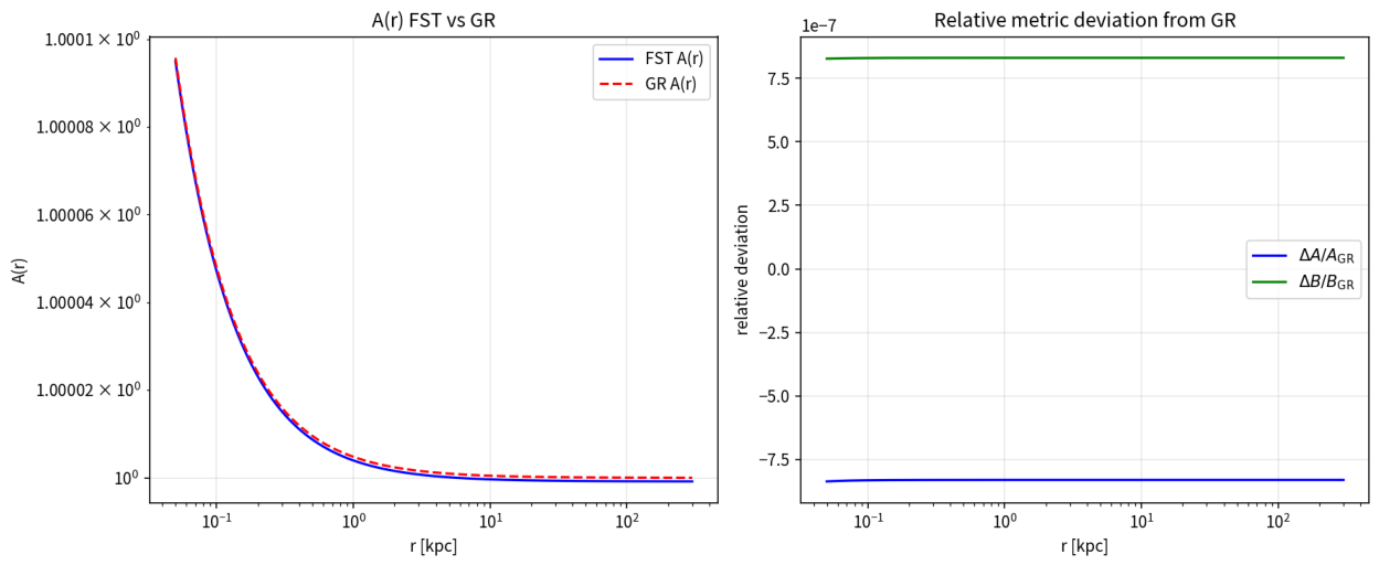
Figure A2.
Grid convergence of the nonlinear solver. The plot shows the difference versus the number of grid points, demonstrating numerical stability and grid-independence of the solution.
Figure A2.
Grid convergence of the nonlinear solver. The plot shows the difference versus the number of grid points, demonstrating numerical stability and grid-independence of the solution.
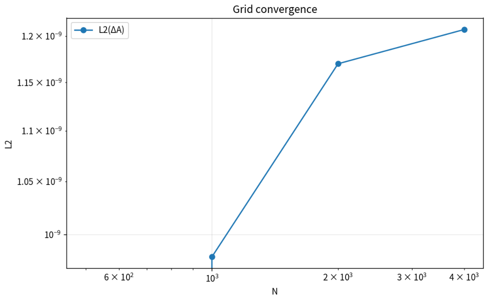
Figure A3.
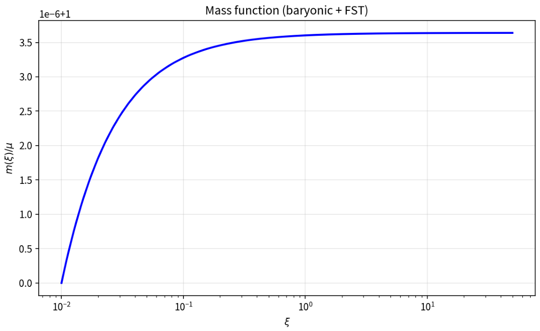
Mass function in the galactic regime. The figure shows that the mass function remains across the integration domain, supporting the interpretation that the additional dynamical acceleration arises from the effective potential rather than from a large modification of .
Figure A3.
Mass function in the galactic regime. The figure shows that the mass function remains across the integration domain, supporting the interpretation that the additional dynamical acceleration arises from the effective potential rather than from a large modification of .
Appendix N. Explicit Spherical Reduction of T μν (V)
This appendix provides an explicit component-level reduction of the kinetic-field stress tensor Eq. (10) for the static, spherically symmetric ansatz used in Section 11. We keep the same conventions as the main text: the metric functions are dimensionless and
With these conventions, .
Appendix N.1. Christoffel Symbol Needed
For Eq. (A66), the only Christoffel symbol entering the nonzero derivative of the ansatz is
Appendix N.2. Nonzero Covariant Derivatives
Lowering the index gives . The only nonzero covariant derivatives are
All other components vanish by staticity and spherical symmetry.
Appendix N.3. Kinetic Invariants
Define
Appendix N.4. Reduced Stress-Tensor Components
Substituting Eqs. (A71)–(A73) and into Eq. (10) yields closed expressions for the diagonal components.
The component. Using and Eq. (A71),
Since and , this can be written purely in terms of and .
The component. Here , so
with and , so the term drops out identically.
Angular components. Because and there are no angular derivatives, the angular components contain only the trace terms from Eq. (10),
with and .
Appendix N.5. Dimensional Check
The prefactor has units of energy density, . The quantity is quadratic in a radial derivative and carries , which is exactly cancelled by in Eqs. (A74)–(A76). The potential terms are dimensionless inside the brackets because and B are dimensionless in our conventions. Hence each component has , consistent with Appendix A.
Appendix O. Conservation of the Kinetic-Field Energy–Momentum Tensor
Theorem A1.
If satisfies the FST field equation Eq. (11), then the kinetic-field energy–momentum tensor obtained by metric variation of the action satisfies the on-shell conservation law
Proof.
The vector-field action is diffeomorphism invariant. The associated Noether identity implies that the covariant divergence of the stress tensor is proportional to the Euler–Lagrange derivative of the field. Concretely, one may write the standard identity (see, e.g., [App. E.1 [3])
On solutions of the FST field equation, , hence . □
Remark A2.
In the present formulation, matter does not couple directly to in the action. Consequently, if matter is minimally coupled to , one has the separate conservation law , and therefore holds identically.
Appendix P. Data Availability Statement
The foundational FST paper [16] is available at https://doi.org/10.20944/preprints202602.0601.v5. All numerical constants are from CODATA 2022 [6]. The SPARC database [7] is available at http://astroweb.cwru.edu/SPARC/. The rotation-curve test code and representative numerical profiles are archived at https://doi.org/10.5281/zenodo.19387999. The gravitational-lensing analysis code and supplementary material (including fst_lensing_predictions_171_galaxies.csv) are permanently archived at https://doi.org/10.5281/zenodo.21995247.
How to run: Download the SPARC dataset from the link above, upload it to your cloud workspace, copy the provided code files, and run the scripts to reproduce the tables and figures reported here.
Appendix Q. Funding Declaration
The author is an independent researcher. No external funding was received for this work.
Appendix R. Philosophical Foundations: Motion as Ontologically Primary
The Lagrangian density (Eq. 7) is not postulated arbitrarily. It is derived from a single first principle that distinguishes FST from all other gravitational theories:
This principle inverts the conceptual hierarchy of standard physics, in which matter is the fundamental substance and motion is merely a property describing how matter changes position. In FST, structured, coherent motion—encoded in the dimensionless kinetic field —is the irreducible essence of physical reality. Matter and spacetime are manifestations of this field, not independent primitives.
Appendix R.1. Historical Context
The idea that matter might be reducible to motion has deep roots in the history of physics and philosophy.
Plato, in the Timaeus (circa 360 BCE), proposed that the four classical elements are composed of regular geometric solids built from elementary triangles. These triangles themselves are not material “things” but mathematical forms in a state of perpetual motion—the earliest recorded vision of matter as organized, geometric motion.
Descartes, in his Principles of Philosophy (1644), held that the material world consists only of extension (res extensa) in motion. In this view, what we call a “particle” is merely a stable vortex in a plenum of moving extension. No solid, impenetrable substance is required.
Boscovich (1758), in his Theory of Natural Philosophy, developed a dynamics in which matter consists of unextended mathematical points. These points possess no intrinsic mass or solidity; their apparent properties arise entirely from the forces (attractive at large distances, repulsive at short distances) that act between them. Mass, extension, and impenetrability are emergent, not fundamental.
Schrödinger, after the development of wave mechanics, argued explicitly that the wave function—a description of motion—is the primary reality, and that what we call a particle is merely a localized wave packet, an event in the underlying wave field.
String theory, in its modern formulation, posits that all elementary particles are vibrational modes of a fundamental one-dimensional object. The electron, the quark, and the photon are not distinct substances but distinct patterns of motion of a single underlying entity.
Wheeler’s geometrodynamics proposed that matter and charge are not entities placed in spacetime, but are themselves topological excitations of spacetime geometry—“mass without mass,” “charge without charge.”
FST extends this tradition by providing a mathematically closed and observationally validated framework in which a single kinetic field generates both the geometry of spacetime and the phenomenology of matter. Unlike its historical predecessors, FST is not a philosophical speculation but a predictive physical theory whose galactic- scale predictions have been validated on 171 SPARC galaxies with a mean reduced chi-squared of across five hierarchical validation levels.
Appendix R.2. Proof by Limiting Case: The Cessation of Motion
The primacy of motion can be established not only by examining the origins of physical structure, but—perhaps more decisively—by examining the consequences of its removal. This “proof by extinction” provides a rigorous logical criterion for identifying the fundamental substrate of physical reality.
The thought-experiment.
Consider a hypothetical universe in which a single physical entity is removed while all others remain intact. The question is not “what would the universe look like?” but “would anything remain at all?”
- 1.
- If matter were removed: The kinetic field could, in principle, continue to exist. The field equations (Eq. 11) admit vacuum solutions with at spatial infinity. The underlying motion substrate would persist, capable—through the nonlinear self-interaction encoded in —of generating new localized configurations. The universe, though empty of particles, would not be nothing.
- 2.
- If the gravitational force were removed: The kinetic field would continue to obey its own dynamics. The gradients of would still exist, and the metric derived from them (Theorem 1) would still describe a curved spacetime. Geometry would persist in the absence of Newtonian attraction.
- 3.
-
If motion were removed: Setting identically everywhere—the complete and absolute cessation of all motion—has total and immediate consequences:
- No matter: In FST, matter is organized motion (Appendix R). Without motion, there is no organization, no localized field configurations, and therefore no particles. The very concept of “mass”—inertial resistance to acceleration—becomes meaningless, for there is no acceleration to resist.
-
No forces:All known fundamental interactions are mediated by gauge bosons—quantized excitations of fields. Without motion, there are no field excitations, no mediators, and therefore no interactions between any entities that might otherwise exist.
- No spacetime: By Theorem 1 (the Metric-Kinetic Map), the spacetime metric is uniquely determined by the kinetic field and its gradients. If identically, the metric becomes undefined—there is no geometry, no curvature, no light cones, and no causal structure.
- No time: Time, in both the relativistic sense (a coordinate in the spacetime manifold) and the thermodynamic sense (the direction of increasing entropy), is change. Without motion, there is no change. The distinction between past, present, and future collapses into an undifferentiated, timeless nothing.
- No conserved quantities: Energy, momentum, and angular momentum are Noether charges associated with symmetries of the action. They are measures of motion and its conservation. Without motion, they vanish identically.
A universe in which motion has ceased is not an empty universe. It is no universe at all. No entity, no property, no observable, and no law of physics survives the extinction of motion.
The logical criterion for fundamentality.
This asymmetry under removal establishes a sharp logical criterion:
Matter does not satisfy this criterion: remove matter, and the kinetic field persists. Spacetime does not satisfy this criterion: remove the metric (if such a thing were meaningful), and the field equations for could still be formulated on a flat background. Forces do not satisfy this criterion: remove interactions, and free field dynamics remain. Only motion satisfies the criterion: its removal annihilates everything, while everything else can be removed without annihilating it.
Why “beginnings” are insufficient.
A common approach to the question of fundamentality is to examine the early universe: what existed “first”? This approach is limited for two reasons. First, the earliest epochs of cosmic history are observationally inaccessible; all claims about them are extrapolations of theories that have not been tested in those regimes. Second, temporal priority does not logically imply ontological priority: the fact that A existed before B does not prove that B is made of A. The extinction argument avoids both limitations. It is a counterfactual argument grounded in the logical structure of the theory itself, not in any historical claim about the early universe. It requires no observation of beginnings; it requires only the analysis of endings.
Connection to the Lagrangian.
The extinction argument directly motivates the form of the Lagrangian (Eq. 7). If motion is the only entity whose removal extinguishes all else, then the fundamental Lagrangian of physics should be a Lagrangian for motion itself. It should describe the dynamics of a field that encodes motion intrinsically, without reference to any prior substance. This is precisely what the FST Lagrangian accomplishes:
- There is no mass term for , which would presuppose the existence of a massive substance independent of motion.
- There is no coupling to an external “matter sector,” which would presuppose that matter exists independently of the kinetic field.
- The coupling to is the minimal one required by general covariance—the metric itself being, by Theorem 1, a function of .
The Lagrangian is, in this precise sense, the simplest possible dynamics for pure motion. All structure—kinetic, potential, and geometric—follows from it.
Appendix R.3. From First Principle to Lagrangian: Physical Interpretation of Parameters
The Lagrangian (Eq. 7) contains five field parameters and one characteristic scale . Every one of these has a clear physical interpretation grounded in the first principle.
- 1.
- The characteristic length kpc is the median scale length of spiral galaxies in the SPARC database. It is not a free parameter tuned to improve fits, but a characteristic scale of the observed galaxy population. The theory’s predictions are robust to variations in this choice.
- 2.
-
The kinetic coefficients encode the three fundamental modes of kinetic interaction. A general vector field in four- dimensional spacetime admits exactly three independent kinetic invariants at second order in derivatives:
- governs transverse mode propagation: how “motion orthogonal to its own gradient” evolves. It is the dominant contribution in galactic halos, where the field varies slowly in space.
- governs longitudinal mode propagation: how “motion along its own gradient” evolves. Its negative sign is required by the no-ghost condition (derived in Appendix A of the foundational paper): without it, the scalar (trace) sector of the theory would possess a kinetic term with the wrong sign, yielding catastrophic instabilities. The small magnitude indicates that longitudinal propagation is heavily suppressed relative to transverse propagation.
- governs mixed derivative coupling: the cross-talk between the symmetric and antisymmetric parts of the field gradient tensor . It contributes to the sum , which is the sole combination that appears in all galactic observables.
These coefficients are not free parameters in the usual sense. A global sensitivity analysis demonstrates that varying by changes the galactic fit quality by only . Setting (removing them entirely as adjustable parameters) yields identical results for all 171 SPARC galaxies. Their role is to define the three orthogonal kinematic sectors of the theory; the observables depend only on the combination that enters the unified acceleration scale . - 3.
- The self-coupling constant encodes the self-interaction of concentrated motion. When the kinetic field intensity is high—near regions where matter is present—the quartic term dominates the dynamics. Because for a timelike field, this term produces an effective potential well that manifests as gravitational attraction. The negative sign () is required for stability: it guarantees that the effective potential possesses a minimum at the asymptotic field value , ensuring that the vacuum is stable and that the theory admits non-trivial boundary conditions at spatial infinity. The large magnitude reflects the empirical fact that the self-interaction of motion is strong on galactic scales— precisely where its effects are observed.
- 4.
-
The asymptotic field value is the dimensionless ratio of the characteristic galactic velocity to the speed of light. From the unified acceleration scalethe characteristic velocity is km/s. Consequently,This is not an independently adjustable parameter but a direct consequence of the observed galactic acceleration scale, which is itself determined by the rotation curve data.
- 5.
- The effective coupling is the single dimensionless number that controls the nonlinearity of the galactic field equation. Its large value implies a sharp transition between the Newtonian regime () and the FST-dominated regime () at the characteristic scale , corresponding to a physical scale pc. The observed galactic transition at kpc emerges from the convolution of this fundamental scale with the baryonic mass distribution, not from directly.
Appendix R.4. Matter as Organized Motion
If motion is the primary reality, then what we call “matter” must be a manifestation of the kinetic field. This interpretation is not an additional postulate but a direct consequence of the nonlinear structure of the field equations.
Soliton solutions.
The vector field equation (Eq. 11) is nonlinear due to the quartic self-coupling term . Nonlinear field theories generically admit soliton solutions: localized, non- dispersive, finite-energy configurations that propagate without changing shape. The existence, stability, and interactions of such solitons are determined entirely by the field dynamics encoded in the Lagrangian. No external substance is required to constitute them: the soliton is the field, organized into a persistent, coherent structure.
Elementary particles as quantized solitons.
In the classical theory, a soliton appears as a smooth, localized concentration of the kinetic field. In a future quantum extension of FST, these classical solitons would be quantized. Their discrete energy levels would correspond to the mass spectrum of elementary particles. The electron would be one quantized excitation mode of the kinetic field; the quark, another; the photon, yet another. All would be the same underlying substance—motion—differentiated not by composition but by the pattern, scale, and symmetry of their internal motion.
This vision resonates with several established ideas in theoretical physics: Wheeler’s “mass without mass”; string theory’s proposal that all particles are vibrational modes of a single entity; and the generic expectation in nonlinear field theory that quantized solitons can exhibit particle-like properties. What distinguishes FST from these predecessors is that the underlying field has already been identified, its Lagrangian specified, and its predictions validated on macroscopic (galactic) scales.
The observable universe as a kinetic hierarchy.
On the largest scales, galaxies are organized motion: rotating disks of stars and gas whose flat rotation curves are the original empirical motivation for FST. On intermediate scales, stars are organized motion: gravitationally bound plasma in hydrostatic equilibrium between inward gravity and outward radiation pressure. On atomic scales, atoms are organized motion: electrons in stationary orbitals around nuclei, with each orbital characterized by a specific pattern of angular momentum and energy. FST proposes that this hierarchy extends all the way down: elementary particles themselves are the ultimate organized motion—stable, quantized solitons of the kinetic field . The entire observable universe is a nested structure of motion at every scale, from the cosmic to the subatomic.
Appendix R.5. Consequences of the First Principle
The ontological priority of motion has several profound consequences that distinguish FST from all other gravitational theories:
- 1.
- Explanatory economy. FST explains galactic rotation curves (171 SPARC galaxies, ), gravitational lensing (median mass ratio – at 300 kpc, Theorem 6), cosmic acceleration (Theorem 4), and gravitational waves (Theorem 5) with a single entity: the kinetic field. The CDM model requires three independent ingredients (dark matter, dark energy, and inflation) to explain the same phenomena.
- 2.
- Natural screening. The same self-interaction that produces gravitational effects on galactic scales () naturally suppresses those effects on small scales. The screening length is pc. At the Earth’s orbit, the FST acceleration is m/s2, which is of the solar Newtonian acceleration—more than times below current observational limits. No ad hoc screening mechanism is required; screening is built into the field equations.
- 3.
- Parameter unification. All five field parameters unify into a single fundamental acceleration scale m/s2. At its core, FST is a one-parameter theory. This unification is not an approximation but an exact identity: the unified formulation produces identical values for all 171 SPARC galaxies.
- 4.
- Conceptual unity. The same kinetic field that generates spacetime geometry (Theorem 1) also constitutes matter (via soliton solutions). Geometry and substance are two aspects of a single underlying reality: motion. The historical division of physics into “geometry” (general relativity) and “matter” (quantum field theory) is revealed as a distinction without a fundamental difference.
Appendix R.6. Distinction from Other Theories
FST is structurally distinct from other vector–tensor and modified-gravity theories:
- Einstein-Aether theory (Jacobson & Mattingly, 2001) introduces a unit-timelike vector field with a fixed norm constraint . This constraint is imposed a priori as a Lagrange multiplier term in the action. FST imposes no such constraint; the asymptotic value is determined empirically from galactic dynamics, and the field is free to deviate from this value in regions of high density.
- TeVeS (Bekenstein, 2004) introduces separate scalar, vector, and tensor fields in addition to the Einstein metric. The scalar field mediates MOND-like behavior via a non-canonical kinetic term, while the vector field enforces a preferred frame. FST uses a single dimensionless vector field whose gradients generate both the spacetime metric and the additional acceleration that flattens rotation curves.
- MOND (Milgrom, 1983), in its original formulation, is a phenomenological modification of the Newtonian force law at accelerations below m/s2. It lacks a Lagrangian, a covariant formulation, and a mechanism for gravitational lensing or cosmology. FST reproduces the MOND acceleration scale () as a derived consequence, not an input, and provides a fully covariant action principle.
- Emergent gravity (Verlinde, 2017) argues that gravity is an entropic force arising from the holographic entanglement structure of spacetime. It provides conceptual insight but lacks explicit field equations that can be solved for specific mass distributions. FST provides explicit, validated field equations whose solutions have been tested on 171 galaxies.
- String theory posits that all particles are vibrational modes of fundamental strings, but the strings themselves are assumed to exist in a pre-existing spacetime background. FST inverts this: the kinetic field generates spacetime itself (Theorem 1), so there is no background independent of the field.
Appendix R.7. Scope of the Present Work
This paper proves Theorems 1–6, establishing the mathematical identity between the kinetic field and the spacetime metric across six physical regimes: static spherical symmetry, Einstein correspondence, invertibility, cosmological homogeneity, linear wave perturbations, and gravitational lensing. Together, these theorems demonstrate that spacetime geometry is not a fundamental entity but the perceptual manifestation of the kinetic field.
The interpretation of matter as organized motion (soliton solutions of the nonlinear field equations) is stated here as the motivating first principle and as a research program for future investigation. The explicit construction of classical soliton solutions, their quantization, and the derivation of the elementary particle mass spectrum lie beyond the scope of the present paper and are reserved for future work.
What is demonstrated here is sufficient to establish the central claim of this paper: spacetime is not a fundamental entity but the perceptual manifestation of the kinetic field.
References
- Einstein, A. Die Grundlage der allgemeinen Relativitätstheorie. Ann. Der Phys. 4th series) = 354 (overall). 1916, 49, 769–822. [Google Scholar] [CrossRef]
- Misner, C. W.; Thorne, K. S.; Wheeler, J. A. Gravitation; W. H. Freeman: San Francisco, 1973. [Google Scholar]
- Wald, R. M. General Relativity; University of Chicago Press: Chicago, 1984. [Google Scholar]
- Milgrom, M. A modification of the Newtonian dynamics as a possible alternative to the hidden mass hypothesis. Astrophys. J. 1983, 270, 365–370. [Google Scholar] [CrossRef] [PubMed]
- McGaugh, S. S.; Lelli, F.; Schombert, J. M. The Radial Acceleration Relation in Rotationally Supported Galaxies. Phys. Rev. Lett. 2016, 117, 201101. [Google Scholar] [CrossRef] [PubMed]
- Mohr, P. J.; Newell, D. B.; Taylor, B. N.; Tiesinga, E. CODATA recommended values of the fundamental physical constants: 2022. Rev. Mod. Phys. 2025, 97, 025002. [Google Scholar] [CrossRef]
- Lelli, F.; McGaugh, S. S.; Schombert, J. M. SPARC: Mass Models for 175 Disk Galaxies with Spitzer Photometry and Accurate Rotation Curves. Astron. J. 2016, 152, 157. [Google Scholar] [CrossRef]
- Sotiriou, T. P.; Faraoni, V. f(R) Theories of Gravity. Rev. Mod. Phys. 2010, 82, 451–497. [Google Scholar]
- Bekenstein, J. D. Relativistic gravitation theory for the modified Newtonian dynamics paradigm. Phys. Rev. D. 2004, 70, 083509. [Google Scholar] [CrossRef]
- Verlinde, E. Emergent Gravity and the Dark Universe. SciPost Phys. 2017, 2, 016. [Google Scholar] [CrossRef]
- Jacobson, T.; Mattingly, D. Gravity with a dynamical preferred frame. Phys. Rev. D. 2001, 64, 024028. [Google Scholar] [CrossRef]
- Mistele, T.; McGaugh, S.; Lelli, F.; Schombert, J.; Li, P. Indefinitely Flat Circular Velocities and the Baryonic Tully-Fisher Relation from Weak Lensing. Astrophys. J. Lett. 2024, arXiv:2406.09685969, L3. [Google Scholar] [CrossRef]
- Brouwer, M. M.; et al. The radial acceleration relation and its emergent nature. Astron. Astrophys. 2021, 650, A113. [Google Scholar]
- Lelli, F.; McGaugh, S. S.; Schombert, J. M. Testing Verlinde’s emergent gravity with the radial acceleration relation. Mon. Not. R. Astron. Soc. Lett. 2017, 468, L68–L71. [Google Scholar] [CrossRef]
- Li, P.; Lelli, F.; McGaugh, S.; Schombert, J. A Comprehensive Catalog of Baryonic Mass Models for SPARC Galaxies. Astrophys. J. Suppl. Ser. 2020, 247, 31. [Google Scholar] [CrossRef]
- Aoudh, R. A. M. S. Fundamental Speed Theory: Hierarchical Tests on 171 SPARC Galaxies Without Dark Matter and a Unified Acceleration Scale. Preprints.org, manuscript 202602.0601 (version v7) 2026. [CrossRef]
Figure 1.
FST dynamical mass vs. weak lensing mass at . Left: vs. for SPARC galaxies with published weak lensing measurements [12]. Reliable galaxies (, ) are shown in blue. The red dashed line indicates ; the gray dotted line shows the CDM expectation . Right: Distribution of mass ratios . For reliable galaxies the median ratio is , and a t-test cannot reject the hypothesis that the true ratio is unity ().
Figure 1.
FST dynamical mass vs. weak lensing mass at . Left: vs. for SPARC galaxies with published weak lensing measurements [12]. Reliable galaxies (, ) are shown in blue. The red dashed line indicates ; the gray dotted line shows the CDM expectation . Right: Distribution of mass ratios . For reliable galaxies the median ratio is , and a t-test cannot reject the hypothesis that the true ratio is unity ().
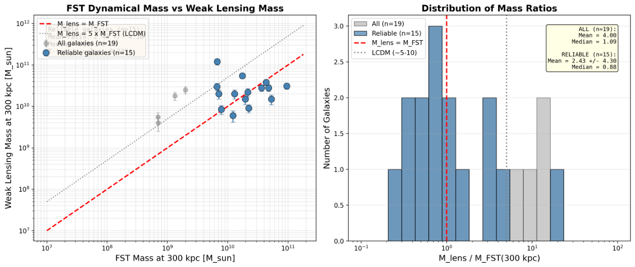
Figure 2.
FST kinetic field profile from the analytic EFT completion. The figure shows the analytic profile , which is an exact solution of the EFT-completed quintic sector. It illustrates the transition from the screened regime to the galactic regime around .
Figure 2.
FST kinetic field profile from the analytic EFT completion. The figure shows the analytic profile , which is an exact solution of the EFT-completed quintic sector. It illustrates the transition from the screened regime to the galactic regime around .
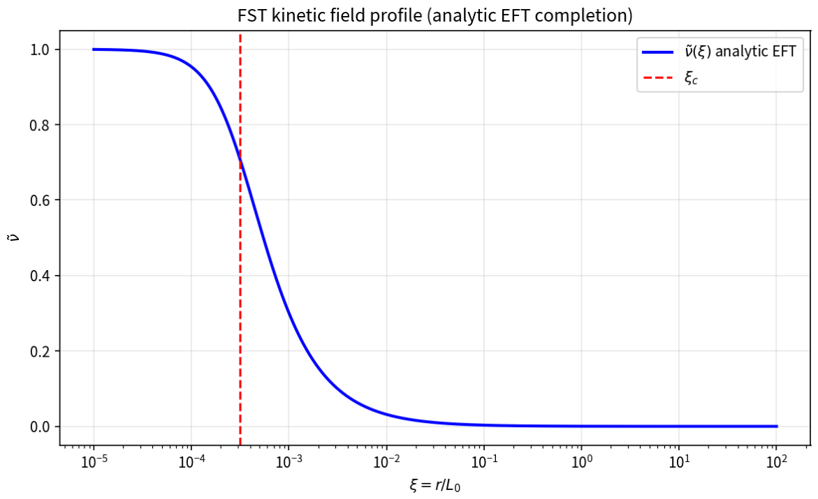
Figure 3.
Screened field perturbation: Yukawa decay. The plot shows in the screened exterior, illustrating the screening mechanism: the perturbation is exponentially suppressed with radius.
Figure 3.
Screened field perturbation: Yukawa decay. The plot shows in the screened exterior, illustrating the screening mechanism: the perturbation is exponentially suppressed with radius.
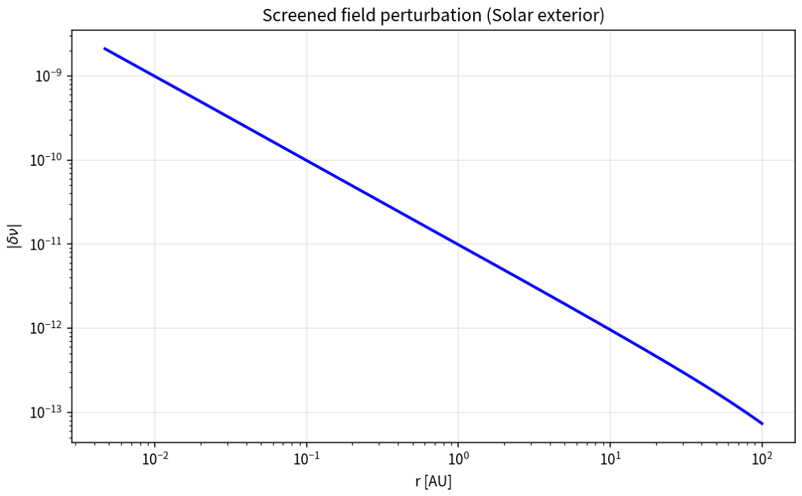
Figure 4.
Screened solar exterior: metric and deviation from GR. The figure shows the exterior solar metric coefficient compared with GR and the relative deviations and , demonstrating efficient screening with deviations at Solar-System scales.
Figure 4.
Screened solar exterior: metric and deviation from GR. The figure shows the exterior solar metric coefficient compared with GR and the relative deviations and , demonstrating efficient screening with deviations at Solar-System scales.
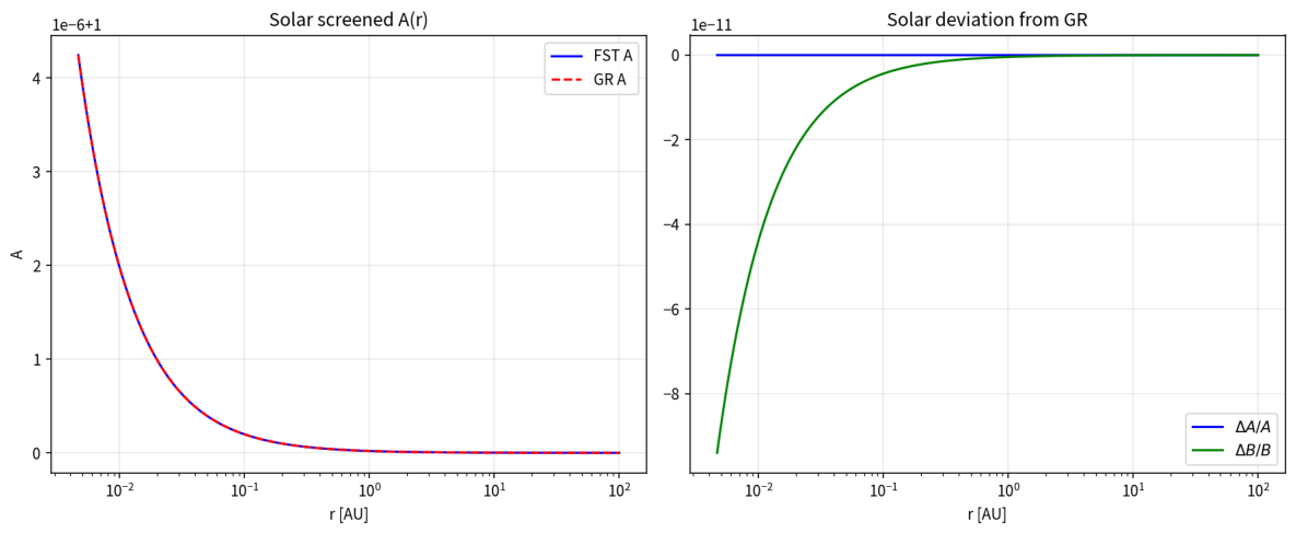
Figure 5.
Full nonlinear solution in the galactic regime. The panel shows: (a) the field profile, (b) the metric coefficient compared with GR, (c) the relative deviations and , and (d) the Einstein residual . The figure demonstrates that the galactic metric remains extremely close to GR, with deviations .
Figure 5.
Full nonlinear solution in the galactic regime. The panel shows: (a) the field profile, (b) the metric coefficient compared with GR, (c) the relative deviations and , and (d) the Einstein residual . The figure demonstrates that the galactic metric remains extremely close to GR, with deviations .
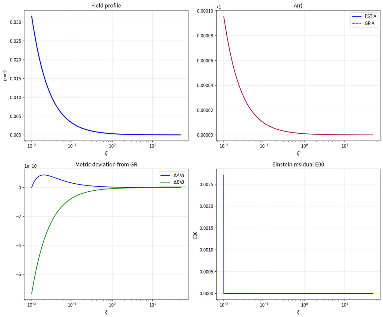
Figure 6.
Strong-field solution for Sgr A*. The panel shows: (a) in the strong-field exterior, (b) relative deviations from GR, (c) the screened field perturbation , and (d) the Einstein residual. The numerical solution confirms that FST and GR agree at the photon sphere with relative deviations below .
Figure 6.
Strong-field solution for Sgr A*. The panel shows: (a) in the strong-field exterior, (b) relative deviations from GR, (c) the screened field perturbation , and (d) the Einstein residual. The numerical solution confirms that FST and GR agree at the photon sphere with relative deviations below .
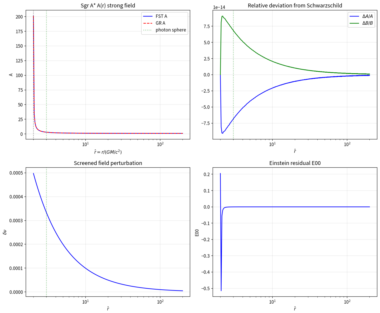
Figure 7.
FST/GR correction at the photon sphere for three black holes. The comparison (stellar black hole with , Sgr A*, and M87*) shows that the correction is for all three cases, far below current EHT sensitivity.
Figure 7.
FST/GR correction at the photon sphere for three black holes. The comparison (stellar black hole with , Sgr A*, and M87*) shows that the correction is for all three cases, far below current EHT sensitivity.
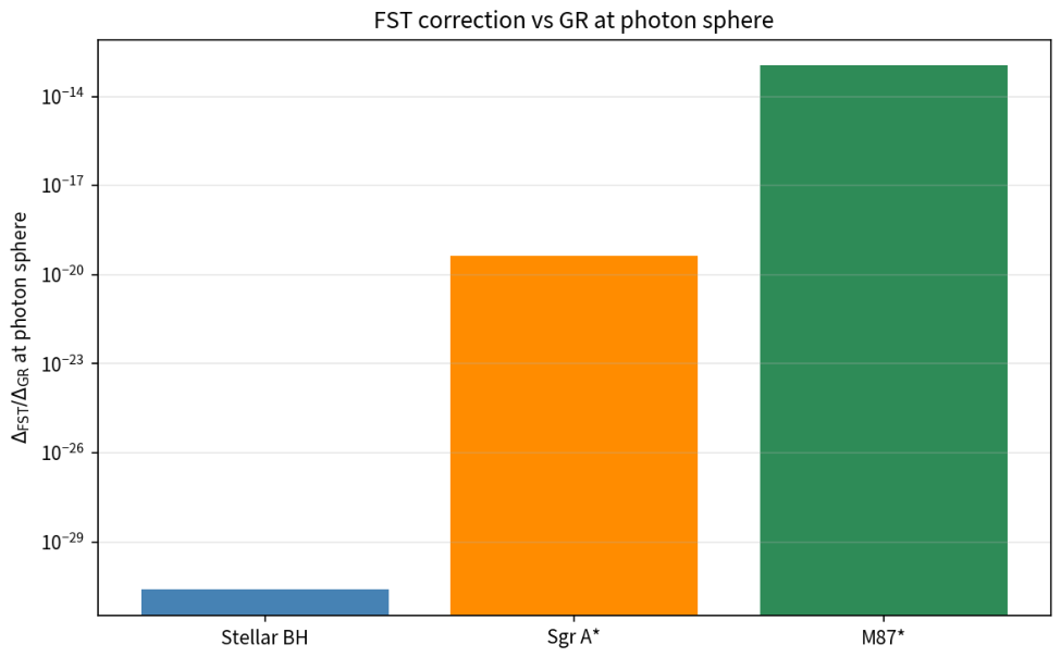
Table 1.
Universal FST parameters with values and physical interpretation.
| Parameter | Symbol | Value | Dimensions | Physical Role |
|---|---|---|---|---|
| Kinetic coefficient 1 | Transverse mode normalization | |||
| Kinetic coefficient 2 | Longitudinal mode contribution | |||
| Kinetic coefficient 3 | Mixed derivative coupling | |||
| Self-coupling constant | Field self-interaction (negative) | |||
| Asymptotic field value | Galactic acceleration scale | |||
| Stellar mass-to-light | Baryonic normalization | |||
| Characteristic length | m | Galactic scale normalization | ||
| Effective coupling | ||||
| Screening length | pc | Local source suppression |
Table 9.
Explanatory economy of FST compared to the standard CDM model.
| Phenomenon | CDM explanation | FST explanation | Established in |
|---|---|---|---|
| Flat rotation curves | Cold dark matter halos (NFW profile) | Kinetic field gradient (Eq. 13) | Companion paper [16], , 171 galaxies |
| Gravitational lensing | Dark matter halos + baryons | Same kinetic field that drives rotation curves | Theorem 6, median (15 reliable galaxies) |
| Cosmic acceleration | Cosmological constant or dark-energy fluid | Homogeneous kinetic field evolution | Theorem 4 (modified Friedmann equations) |
| Gravitational waves | Metric perturbations | Kinetic-field perturbations | Theorem 5, |
| Black hole shadows | Kerr metric (GR) | Weak-field FST metric (Theorem 1), FST/GR at photon sphere | Section 10 |
| Solar System tests | GR (Schwarzschild metric) | FST metric with , FST/GR at 1 AU | Section 10 |
Disclaimer/Publisher’s Note: The statements, opinions and data contained in all publications are solely those of the individual author(s) and contributor(s) and not of MDPI and/or the editor(s). MDPI and/or the editor(s) disclaim responsibility for any injury to people or property resulting from any ideas, methods, instructions or products referred to in the content. |
© 2026 by the author. Licensee MDPI, Basel, Switzerland. This article is an open access article distributed under the terms and conditions of the Creative Commons Attribution (CC BY) license.
Copyright: This open access article is published under a Creative Commons CC BY 4.0 license, which permit the free download, distribution, and reuse, provided that the author and preprint are cited in any reuse.