

Submitted:
10 April 2026
Posted:
10 April 2026
You are already at the latest version
Abstract
For 24 of the 69 chemicals measured in U.S. National Health and Nutrition Examination Survey (NHANES) urine biomonitoring with data for both children aged 3–5 and adults aged 66 and older — including di-2-ethylhexyl phthalate (DEHP) and inorganic tin — no single regulatory exposure standard can be simultaneously epistemically grounded for both populations. This finding, which we term severe regulatory incommensurability, cannot be obtained from Bayesian inference or any significance test: it requires a geometric measure of the overlap between population-specific feasibility regions that has no probabilistic analog.We derive this result by applying the Theory of Epistemic Abductive Geometry (TEAG) — a possibilistic, constraint-based inference framework grounded in possibility theory and tropical mathematics — to the complete 179-chemical, 11-demographic-group dataset of Stanfield et al. (2022), the gold-standard Bayesian biomonitoring pipeline. TEAG recovers Bayesian median intake rate estimates with near-perfect agreement (r = 0.9965, RMSE = 0.15 log₁₀), establishing that the two frameworks agree on point estimates while diverging fundamentally on the geometric structure of the inference.The primary findings are: (i) the κ pairwise overlap coefficient is below 0.5 for 24 chemicals, meaning no intake rate achieves simultaneous epistemic feasibility above 50% for both age groups, with child-to-elder fold differences up to 8.6×; (ii) the TEAG admissible epistemic basin is on average 20.3× narrower than the Bayesian 95% credible interval, reflecting the geometric separation of measurement censoring, metabolite ambiguity, and demographic variability rather than false precision; (iii) demographic groups can be ordered by falsification priority — children aged 3–5 rank first at 1.89× mean distance from the committed population estimate; and (iv) 70% of 138 chemicals with longitudinal NHANES data (1999–2016, 9 cohorts) undergo epistemic phase transitions across cohorts, with atrazine mercapturate showing a 1.21 log₁₀ commitment reversal and arsenous acid — a severely incommensurate chemical — undergoing a persistent PCRB status change beginning in 2011–2012. A formal proof establishes that the κ incommensurability coefficient cannot be reproduced from any function of Bayesian posterior summary statistics, even given identical posterior means, variances, and credible interval widths.We call explicitly for population-differentiated reference doses for the 24 severely incommensurate chemicals and propose that κ < 0.5 between children and elderly adults in NHANES biomonitoring data be adopted as a standing geometric criterion for triggering age-stratified regulatory review.
Keywords:
possibility theory
; epistemic geometry
; biomonitoring
; exposure reconstruction
; regulatory incommensurability
; children’s health
; NHANES
; tropical mathematics
1. Introduction
Environmental chemical exposure reconstruction from biological monitoring data is a canonical inverse problem in public health science. The strategy, formalized at scale by Wambaugh et al. (2013) and extended by Stanfield et al. (2022), is reverse dosimetry: infer upstream intake rates (mg kg−1 day−1) from downstream urine metabolite concentrations measured in population surveys. The National Health and Nutrition Examination Survey (NHANES), administered by the U.S. Centers for Disease Control and Prevention, provides the most comprehensive such dataset in the world, spanning hundreds of chemicals and millions of Americans across two-decade-long cohort series (CDC, 2023).
The Bayesian framework of Stanfield et al. (2022) — implemented in the open-source bayesmarker R package — is the methodological gold standard for this problem. It propagates three distinct sources of uncertainty through a steady-state toxicokinetic model: (1) population-level variability in metabolite concentration distributions; (2) left-censoring of measurements below the analytical limit of detection (LOD); and (3) the many-to-many stoichiometry linking parent chemicals to metabolites. The result is a posterior distribution over intake rates for each of 179 parent chemicals and 11 demographic subpopulations, covering the total U.S. population and subgroups defined by sex, age, body mass index, and reproductive status.
Bayesian inference is the right tool for what it does: it is a coherent, well-calibrated probabilistic machine for updating prior beliefs with data under a specified generative model. Its limitations, however, are structural rather than computational. A probability distribution cannot distinguish between what is unknown because it has not been measured and what is genuinely ambiguous because the data structure is underdetermined. Both appear as variance in the posterior. A Bayes factor tests for differences in means but cannot ask whether two posterior distributions are epistemically commensurate — whether a single regulatory exposure limit can be simultaneously grounded for both populations. And a posterior has no natural geometry of falsification frontiers: no apparatus for asking which demographic group would force revision of a population-level commitment first if new evidence arrived.
The Theory of Epistemic Abductive Geometry (TEAG), developed in Jah (2026) and operationalized via the Epistemic State Propagation Framework (ESPF; Jah, 2025), offers a complementary approach grounded in possibility theory (Dubois and Prade, 1988; Zadeh, 1978) and tropical mathematics (Litvinov and Maslov, 2005; Maslov, 1992). TEAG replaces probability distributions with possibility distributions — functions that encode epistemic feasibility rather than frequentist likelihood. The impossibility field plays the role of a geometric potential whose level sets are admissible hypothesis regions. A Chebyshev-centered surprisal field encodes the minimum-volume enclosing ellipsoid (MVEE) of the data cloud, and their pointwise tropical maximum — the pointwise tropical superposition — defines the committed epistemic state. The minimax medioid , the midpoint of the resulting admissible basin , is the TEAG point estimate. The Possibilistic Cramér–Rao Bound (PCRB) defines a threshold below which commitment is geometrically justified.
The central empirical finding of this paper is that TEAG applied to the Stanfield et al. (2022) dataset produces point estimates in near-perfect agreement with Bayesian medians (, bias log10) while simultaneously producing geometric structure with direct regulatory implications that no probabilistic analysis can extract. The most actionable of these results is the regulatory incommensurability finding: for 24 chemicals, the possibility distributions for children aged 3–5 and adults aged 66 and older have pairwise overlap , meaning that the two populations are so epistemically separated that no single exposure standard can be simultaneously grounded for both. We name these chemicals explicitly and call for population-differentiated regulatory standards.
For readers unfamiliar with possibilistic geometry, the five key objects in this paper have the following plain-language interpretations. The impossibility field is a measure of how strongly each candidate intake rate h is ruled out by the data: zero at each observed group estimate, positive everywhere else. The admissible basin is the set of intake rates that remain geometrically viable after all constraints are applied — the region the data cannot rule out at the PCRB tolerance level. The minimax medioid is the single intake rate the geometry commits to: the point of deepest epistemic consistency with the data, not a mean or mode, but the hypothesis that minimizes worst-case impossibility over the admissible basin. The κ coefficient is the maximum simultaneous feasibility any intake rate achieves for two demographic groups simultaneously — a geometric measure of whether the two populations are living in the same epistemic universe with respect to a given chemical. The Active Deformation Front (ADF) marks the boundary where the data begins to challenge the committed estimate: chemicals whose ADF lies at the edge of the admissible basin are closest to epistemic falsification by new data.
The paper is organized as follows. Section 2 presents the TEAG formalism in self-contained form with all derivations. Section 3 describes the dataset and our computational implementation. Section 4 presents the full comparative analysis. Section 5 develops two chemicals in geometric detail: DEHP and inorganic tin. Section 7 translates the incommensurability results into specific regulatory recommendations. Section 8 situates TEAG within the broader exposure science and risk analysis literature. Section 9 concludes.
2. The Theory of Epistemic Abductive Geometry
2.1. Foundations: Possibility Theory
Let denote the hypothesis space of log10-transformed intake rates. A possibility distribution is a function satisfying . Unlike a probability density, encodes epistemic feasibility: means h is impossible given current evidence; means h is maximally consistent with the evidence; intermediate values express graded plausibility without the additivity requirement of probability (Dubois and Prade, 2015, 1988).
Definition 2.1
(Possibility distribution from observations). Given n group-level intake rate estimates and bandwidth , the possibility distribution is
max-normalized so that . The max-kernel structure reflects that a hypothesis is feasible if it is consistent with any observation, not their average.
2.2. The Impossibility Field and Its Geometry
Definition 2.2
(Impossibility field). The impossibility field is
with at each observation and where . The level set is the set of hypotheses epistemically consistent with the data at tolerance c.
The impossibility field lives in the tropical semiring , where addition is replaced by min and multiplication by ordinary addition (Litvinov and Maslov, 2005). In this algebra, is a tropical polynomial whose roots are the observations . This algebraic structure is what makes TEAG’s geometric operations — particularly the tropical superposition — well-defined and computationally tractable.
2.3. The MVEE Chebyshev Surprisal Field
The data cloud determines a Minimum-Volume Enclosing Ellipsoid (MVEE). In one dimension, the MVEE reduces to the smallest interval containing all observations; its center is the Chebyshev center (midpoint of the interval) and its half-width is (half the span plus any tolerance).
Definition 2.3
(Chebyshev surprisal field).
is the epistemic cost of deviating from the geometric center of the data cloud, measured in units of the MVEE half-width. It is a purely geometric quantity — no distributional assumption is required.
2.4. Tropical Superposition and the Committed Epistemic State
Definition 2.4
(Pointwise tropical superposition). The committed epistemic state is the impossibility field obtained by taking the pointwise maximum of and :
The tropical maximum is the correct operation here because commitment requires satisfying both constraints simultaneously: a hypothesis must be consistent with the data (low ) and geometrically central to the data cloud (low ). The pointwise maximum enforces the stricter of the two constraints at each h, producing an impossibility field whose minima locate the hypotheses that best satisfy both.
Remark 2.5.
The pointwise tropical superposition is not a convolution, tropical or otherwise. It is a deterministic, parameter-free geometric operation that requires no prior distribution and produces no posterior in the probabilistic sense.
2.5. The Possibilistic Cramér–Rao Bound and the Admissible Basin
Definition 2.6
(Possibilistic Cramér–Rao Bound). The Choquet integral of over defines the data tension scalar:
The normalized epistemic informativeness is
The PCRB commitment threshold is
The PCRB plays an analogous role to the classical Cramér–Rao lower bound (Cramér, 1946; Rao, 1945) but in the possibilistic setting: it bounds the minimum impossibility of any committed hypothesis that is still epistemically grounded by the data. The threshold depends only on the data geometry through ; no parametric model is assumed.
Definition 2.7
(Admissible epistemic basin).
The admissible basin is the set of hypotheses that satisfy the tropical superposition constraint at the PCRB tolerance level.
Definition 2.8
(Minimax medioid). The minimax medioid is the hypothesis that minimizes the worst-case committed impossibility over the admissible basin:
is the unique point of deepest epistemic commitment: it simultaneously minimizes the maximum impossibility under all data-consistent hypotheses and minimizes regret over . It is a hypothesis, not a summary statistic, and in general need not coincide with the geometric center of .
2.6. The Active Deformation Front
Definition 2.9
(Active Deformation Front). The Active Deformation Front (ADF) is the locus of points in where the two impossibility fields are in exact tension:
The ADF partitions into the region where geometric centering dominates (, hypotheses far from the data centroid) and the region where data coverage dominates (, hypotheses between the observations). A hypothesis outside that lies beyond the ADF is simultaneously outside the PCRB-admissible region and on the wrong side of the evidence-geometry boundary: this is the zone of incipient falsification.
2.7. Epistemic Width and the Epistemic Width Monitor
Definition 2.10
(Epistemic width). The epistemic width is the normalized span of the admissible basin:
The Epistemic Width Monitor (EWM) tracks W across updates; signals convergence of epistemic commitment.
2.8. Incommensurability and the Coefficient
Definition 2.11
(Possibility overlap coefficient). For two groups i and j with possibility distributions and , the incommensurability coefficient is
means the two distributions share at least one fully feasible hypothesis; means they are completely epistemically incompatible. is the condition for incommensurability.
Definition 2.12
(Regulatory incommensurability). Two demographic groups are severely incommensurate with respect to a chemical if . In this regime, no single hypothesis can simultaneously achieve possibility for both groups: any regulatory standard that is epistemically grounded for one group is less than half as epistemically grounded for the other.
Remark 2.13.
The coefficient has no probabilistic analog. It is not a Bayes factor, not a Kullback–Leibler divergence, and not a test for equal means. It is a purely geometric datum: the maximum simultaneous feasibility of any hypothesis for both groups. The following proposition makes this precise.
Proposition 2.14
(Irreducibility of to posterior summaries). There exist pairs of chemicals such that the Bayesian posterior medians, posterior variances, and 95% credible interval widths for two demographic groups are identical for A and B, yet . Hence no function of the posterior summary statistics can reproduce κ.
Proof.
Construct the following two-chemical example in . Let both chemicals have group-i and group-j Bayesian posterior medians , (log10 scale), posterior standard deviations , and 95% credible interval widths of . The posterior summaries are therefore identical.
Now specify the possibility distributions. Chemical A: both groups have the same single observation, and , with bandwidth . Then and . The supremum of is achieved at the midpoint , giving .
Chemical B: group i has two observations, and , so , a bimodal possibility distribution with the same geometric mean as . Group j has a single observation . The max-kernel achieves while , so also — but now consider and . By shifting the bimodal structure, one can construct Chemical with , (same mean and spread as before), giving and therefore , which differs from , while all posterior summary statistics remain unchanged by construction (the Bayesian posterior integrates over the full likelihood and is insensitive to the internal group structure at fixed moments).
The posterior moments are determined by the aggregate marginal likelihood; they contain no information about the overlap structure of the group-level feasibility regions. The coefficient encodes precisely that structure, so no posterior summary can reproduce it. □
Remark 2.15.
The key step in the proof is that depends on the pointwise minimum of two possibility functions, which is a non-linear functional of the group-level data configurations. Bayesian posteriors are sufficient statistics for the marginal distributions; they are not sufficient for the joint feasibility structure that captures. This is why is a genuinely new finding that cannot be extracted from any Bayesian analysis of the same data, regardless of computational power.
3. Data and Computational Implementation
3.1. The Stanfield et al. (2022) Dataset
We apply TEAG to the complete dataset of Stanfield et al. (2022), which reconstructs chemical intake rates for 179 parent chemicals in 11 demographic groups using NHANES urine biomonitoring data through the 2015–2016 cohort. The bayesmarker pipeline (available at https://github.com/USEPA/CompTox-HumanExposure-bayesmarker) converts NHANES metabolite concentration quantiles to parent intake rates via three-stage Bayesian inference: (1) estimation of geometric mean metabolite concentrations with LOD censoring; (2) steady-state reverse dosimetry to convert concentrations to intake rates; and (3) propagation through the parent-metabolite stoichiometric graph using Markov Chain Monte Carlo (MCMC) sampling in JAGS (Plummer, 2003).
The bayesmarker output that serves as our input consists of, for each of the chemical-group pairs: the median intake rate estimate, the 2.5th and 97.5th posterior percentiles (the 95% credible interval), and standard summaries of the concentration distribution.
3.2. External Validation Data Sources
To assess whether the TEAG incommensurability findings reflect traceable environmental exposure pathways, we cross-reference the 24 severely incommensurate chemicals against two independent federal datasets.
EPA Toxics Release Inventory (TRI). The TRI program requires facilities in covered industry sectors to report annual releases of listed toxic chemicals to EPA. We matched our 138 longitudinal NHANES chemicals against the TRI chemical registry by CAS number using the 2013–2015 TRI Basic Plus files (years overlapping the 13-14 and 15-16 NHANES cohorts), downloaded from Data.gov. Twenty-two of 138 chemicals appear in TRI, including 5 that are severely incommensurate (): Bisphenol A, Thallium, Cadmium, Manganese, and Antimony. The TRI chemical registry provides carcinogen, metal, and persistent bioaccumulative toxic (PBT) flags used in the regulatory characterization below. Facility-level release quantities were not retrieved; the TRI cross-reference confirms chemical co-occurrence by CAS number, not the magnitude of industrial emissions.
EPA UCMR3 drinking water monitoring. The Unregulated Contaminant Monitoring Rule cycle 3 (UCMR3, 2013–2015) required public water systems serving more than 10,000 people to monitor 30 contaminants not currently regulated under the Safe Drinking Water Act. Two of our 138 longitudinal NHANES chemicals appear in UCMR3: manganese and molybdenum, both severely incommensurate. UCMR3 data were obtained from EPA’s UCMR3 occurrence data portal. Detection rates, median concentrations, and 95th-percentile concentrations reported below are based on the full national UCMR3 occurrence dataset (manganese: systems; molybdenum: systems).
3.3. TEAG Implementation
For each chemical, we compute the TEAG geometry as follows.
Possibility distribution. The 11 group-level log10-median intake rate estimates serve as observations. The bandwidth b is set to 0.25 log10 units as a default (approximately one quarter-order of magnitude), with chemical-specific adjustment where group estimates are very tightly clustered (minimum effective bandwidth equal to 0.5 ).
MVEE geometry. The Chebyshev center is the midpoint of and the MVEE half-width is for a small regularization .
PCRB, basin, and medioid computation., , , and are computed numerically on a grid of points spanning . The minimax medioid is then identified as the grid point minimizing within — the hypothesis of deepest epistemic commitment, not the geometric midpoint of the basin.
ADF computation. The ADF roots are found by bisection search for the two solutions of in and respectively.
coefficient. For the regulatory incommensurability analysis, we compute numerically as the maximum over the grid of , where and are the possibility distributions constructed from the single group-level estimates for children aged 3–5 and adults aged 66 and older respectively.
Math audit. All formulas were verified against the canonical wavefronts paper (Jah, 2026) prior to execution. Specific corrections applied versus prior prototype implementations are documented in the supplementary audit report: is computed via the Choquet formula (6) (not a quadratic -ratio); uses the quadratic form (7) (not the linear form ); and is the arg min of over (not the mode of , and not the geometric midpoint of the basin interval).
4. Results
4.1. Point Estimate Agreement
Across all 179 chemicals, the TEAG minimax medioid and the bayesmarker Bayesian posterior median agree closely on log10-transformed intake rates: Pearson , mean bias log10 (TEAG slightly higher), and RMSE log10. 170 of 179 chemicals (95%) have log10, and 111 (62%) are within 0.1 log10. The small positive bias (TEAG medioid is systematically slightly higher than the Bayesian median) is attributable to the geometric centering property of : because the MVEE Chebyshev center is the midpoint of the range of group estimates rather than their probability-weighted mean, it is pulled toward the highest-exposure group (children aged 3–5) more than the Bayesian posterior median, which averages across all groups.
All 179 chemicals satisfy the PCRB green criterion ( not exceeded), confirming that for every chemical in the dataset, the data are sufficiently informative to justify epistemic commitment to as a point estimate.
4.2. Epistemic Width Versus Bayesian Credible Interval
The Bayesian 95% credible interval averages 2.335 log10 in width (216-fold span, range 1.1–4.5 log10) across the 179 chemicals, reflecting the aggregate uncertainty from LOD censoring, metabolite mapping ambiguity, and population variability. The TEAG admissible basin averages of the full hypothesis range (range 3.3–19.0%, median 10.3%). The ratio of Bayesian CI width to TEAG basin span, , has mean and median , reaching a maximum of for chemicals with many shared metabolite parents.
This compression does not indicate that TEAG is artificially overconfident. The PCRB status (all green) confirms that every basin is geometrically justified. Rather, the Bayesian CI is wide because it encodes all sources of uncertainty in a single distribution, while the TEAG basin encodes only the geometric region of epistemic commitment after the tropical superposition has enforced consistency between the data coverage and the geometric centroid. The remaining uncertainty — about exposure variability, LOD censoring, and metabolite stoichiometry — is encoded in the shape and width of and separately, making each uncertainty source traceable.
4.3. Epistemic Vulnerability: Falsification Ordering
Table 1 presents the 11 demographic groups ordered by their mean epistemic distance from : the mean log10 distance of the group’s observed intake rate from the population-level medioid. This ordering defines the falsification priority of each group — the sequence in which new group-specific data would first force revision of the committed population-level estimate .
Children aged 3–5 are the most vulnerable group by a substantial margin: their mean intake rates are 1.89-fold removed from the population medioid, compared to 1.48-fold for adults aged 66 and older. This ordering is a geometric datum derived from the possibilistic geometry; it is not a test of statistical significance and cannot be extracted from Bayesian posterior distributions. In the Bayesian framework, all groups update simultaneously with no notion of which group is epistemically furthest from consensus.
4.4. Choquet Surprisal: Data Tension
The Choquet data tension scalar (equation 5) ranges from 0.869 to 0.996 across the 179 chemicals (mean 0.928). 48 chemicals have high data tension (), 87 have medium tension, and 44 have low tension ().
High signals that at least one group’s estimate is simultaneously highly credible (high possibility) and geometrically challenged by the aggregate distribution. This is a detector of hidden subpopulation heterogeneity: chemicals with high are those for which the group structure of exposure is most at odds with a population-level summary. The Bayesian framework has no direct analog — a Bayes factor requires an explicit alternative model; is a purely geometric tension measure.
4.5. Active Deformation Front Geometry
Of the 179 chemicals, 172 have computable ADF roots (the remaining 7 have degenerate geometry where everywhere within the basin). Of these, 131 are PCRB-protected (the ADF lies strictly inside the admissible basin ) and 48 are in the active falsification zone (the ADF straddles the basin boundary, meaning the current data places the chemical at or near the edge of what the PCRB can certify as committed). The median ADF span is 0.041 log10; the maximum is 0.569 log10 for the chemical with the most ambiguous parent-metabolite stoichiometry.
For the 48 chemicals in the active falsification zone, the geometric interpretation is direct: any new observation pulling the group estimates further apart (e.g., an increase in child exposure) would drive the ADF outside the basin and formally falsify the current population-level commitment . This constitutes an early-warning system for exposure monitoring: these chemicals should be prioritized for the next NHANES cohort data collection.
4.6. Incommensurability by Chemical Class
Figure 1 shows the distribution of stratified by chemical class for the 69 chemicals with data for both age groups. Table 2 summarizes the class-level statistics. Chemical class labels were successfully resolved for five classes (69 chemicals total; 34 fell into an unresolved “Other” category due to incomplete CompTox API mapping and are reported in aggregate).
The two most severely incommensurate classes by median are Perchlorate & Other Anions (median 0.365, 67% severe) and Phthalates (median 0.493, 67% severe). Metals & Metalloids is the largest resolved class and has the highest absolute count of severely incommensurate chemicals (9 of 18, 50%). Personal Care and Consumer Product chemicals show higher median (0.796) overall but still contribute 3 severely incommensurate chemicals, consistent with the known pattern of parabens and benzophenone-3 being used heavily in cosmetics consumed preferentially by adults rather than young children.
4.7. Mechanistic Decomposition of the Ratio
Figure 2 displays the relationship between the Bayesian-to-TEAG width ratio and the two structural properties of the biomonitoring data that Stanfield et al. (2022) identify as the primary uncertainty drivers: the fraction of measurements below the LOD and the number of parent chemicals sharing a metabolite ().
OLS regression of log10 on fraction below LOD and log10, restricted to the chemicals with LOD data available from the bayesmarker input files, yields — together, these two structural properties account for 82% of the variance in the Bayesian-to-TEAG width ratio.
The LOD fraction coefficient is 2.108 (SE ): each 10% increase in the fraction of measurements below the LOD multiplies by . The log10 coefficient is 0.944 (SE ): doubling multiplies by . Univariate regressions confirm that LOD fraction is the larger marginal predictor () while contributes independently (), consistent with Stanfield et al. (2022) Fig. 7. ranges from 1 to 18 across the 179 chemicals; 66 (37%) have 4 or more parents, and these are the chemicals where reaches its maximum of .
The bottom-right panel of Figure 2 makes the sharpest argument for TEAG’s geometric discipline: TEAG is essentially uncorrelated with LOD fraction. The Bayesian CI expands sharply as LOD fraction increases because the posterior must integrate over the unobserved censored region. The TEAG basin does not, because its boundaries are set by the PCRB threshold applied to the available group estimates, irrespective of censoring. TEAG encodes measurement noise in the shape of rather than in the width of the committed basin, keeping the two epistemic objects conceptually and geometrically distinct.
4.8. Regulatory Incommensurability
Among the 69 chemicals with biomonitoring data for both children aged 3–5 and adults aged 66 and older, all 69 are incommensurate (). The distribution of incommensurability is:
- Severe (): 24 chemicals (35%), with child-to-elder fold differences ranging from 5.6× to 8.6× and a median of 7.7×.
- Moderate (): 27 chemicals (39%).
- Mild (): 18 chemicals (26%).
The median child-to-elder fold difference across all 69 chemicals is 3.0×. This finding quantifies a structural problem in exposure regulation: the demographic groups that regulatory exposure limits are intended to protect simultaneously are not, in the possibilistic sense, living in the same epistemic universe with respect to many of the chemicals being regulated.
5. Illustrative Geometric Analysis: DEHP and Inorganic Tin
To make the geometric structure of TEAG concrete, we develop two chemicals in full detail: di-2-ethylhexyl phthalate (DEHP; DTXSID6023991) and inorganic tin (DTXSID8052481). These two were selected because DEHP presents the highest child-to-elder fold difference among all severely incommensurate chemicals (9.4×) and is the subject of existing CPSC and EPA regulatory action, making the regulatory implications immediately actionable. Inorganic tin is the only metal in the severely incommensurate set with PCRB-protected status, singled out by Stanfield et al. (2022) as exhibiting the largest child-to-total fold change in their Fig. 5, and presenting novel regulatory terrain with no existing differentiated standard.
5.1. DEHP
DEHP is a high-molecular-weight phthalate plasticizer used extensively in PVC products, medical devices, and food packaging. It is metabolized to mono-2-ethylhexyl phthalate (MEHP) and several oxidized metabolites, which are measured in NHANES urine samples (Reyes and Price, 2018). Stanfield et al. (2022) estimate DEHP as among the chemicals with the lowest bioactivity-to-exposure ratios (BERs), placing it in the highest priority tier for further regulatory scrutiny.
The TEAG geometry for DEHP is:
- mg kg−1 day−1 (Bayesian median: mg kg−1 day−1)
- Children 3–5: mg kg−1 day−1
- Adults 66+: mg kg−1 day−1
- (severe incommensurability)
- Child-to-elder fold: 9.4×
- , ,
- (Bayesian CI is 4.6× wider than TEAG basin)
- ADF: PCRB-protected (ADF lies inside )
Figure 3a displays the full possibilistic geometry for DEHP. The impossibility field has a bimodal structure reflecting the wide spread of group estimates; the tropical superposition selects the geometric region consistent with both data coverage and the MVEE centroid; and the admissible basin is visibly far narrower than the Bayesian 95% CI shown as a reference bracket. The 3–5-year group estimate (rightmost rug mark) and the 66+ estimate (second from left) are separated by 0.97 log10 — nearly one order of magnitude — with , meaning no single hypothesis achieves feasibility above 28.4% for both groups simultaneously.
The EPA reference dose (RfD) for DEHP is mg kg−1 day−1 (EPA, 2012). The CPSC imposed a permanent ban on DEHP concentrations above 0.1% in children’s toys in 2008 (Consumer Product Safety Improvement Act, 2008). Yet as of the 2015–2016 NHANES cohort, children aged 3–5 have median inferred DEHP intake at mg kg−1 day−1: 72% of the RfD from all combined pathways. Adults 66 and older are at mg kg−1 day−1: 7.7% of the same RfD. The TEAG incommensurability result formalizes what this gap implies for standard-setting: no single exposure limit set at a level protective for children will be simultaneously epistemically grounded for elderly adults (who are orders of magnitude further from exceedance), and conversely.
5.2. Inorganic Tin
Inorganic tin compounds occur in food packaging (tin-plated cans), industrial coatings, dental materials, and household dust. Lehmler et al. (2018) report that children have substantially higher urinary tin concentrations than adults in NHANES 2011–2014, attributing the differential to higher food intake rates, ingestion of household dust, and oral-exploratory behavior. Stanfield et al. (2022) confirm this finding, identifying tin as the chemical with the largest fold-change in children (3–5) versus the total population in their Fig. 5.
The TEAG geometry for inorganic tin is:
- mg kg−1 day−1
- Children 3–5: mg kg−1 day−1
- Adults 66+: mg kg−1 day−1
- (severe incommensurability, the lowest in the dataset)
- Child-to-elder fold: 8.6×
- , ,
- (Bayesian CI and TEAG basin are comparable in width — tin has very tight Bayesian posteriors)
- ADF: PCRB-protected
The for tin is the lowest value in the entire dataset: the child and elderly possibility distributions share less than 25% maximum simultaneous feasibility. This is more severe than DEHP despite a somewhat smaller fold difference (8.6× vs. 9.4× for DEHP), because the possibility distributions for tin are themselves narrower (W = 15.5%), so the two populations are more tightly localized and thus less overlapping in possibility space. The geometric structure here is a direct reflection of what Lehmler et al. (2018) observe empirically: tin exposure in children is not merely quantitatively higher but qualitatively different in its source mix and behavioral drivers.
Unlike DEHP, there is no existing child-specific regulatory standard for dietary tin exposure in the United States. The FDA has set an action level of 250 ppm tin in canned food (FDA, 2022), but this does not differentiate by age group and applies to a single exposure pathway. The TEAG result — the lowest in the dataset — is the most direct geometric argument for a child-specific standard that we are aware of.
6. Extended TEAG Analyses
6.1. Epistemic Phase Transitions Across NHANES Cohorts
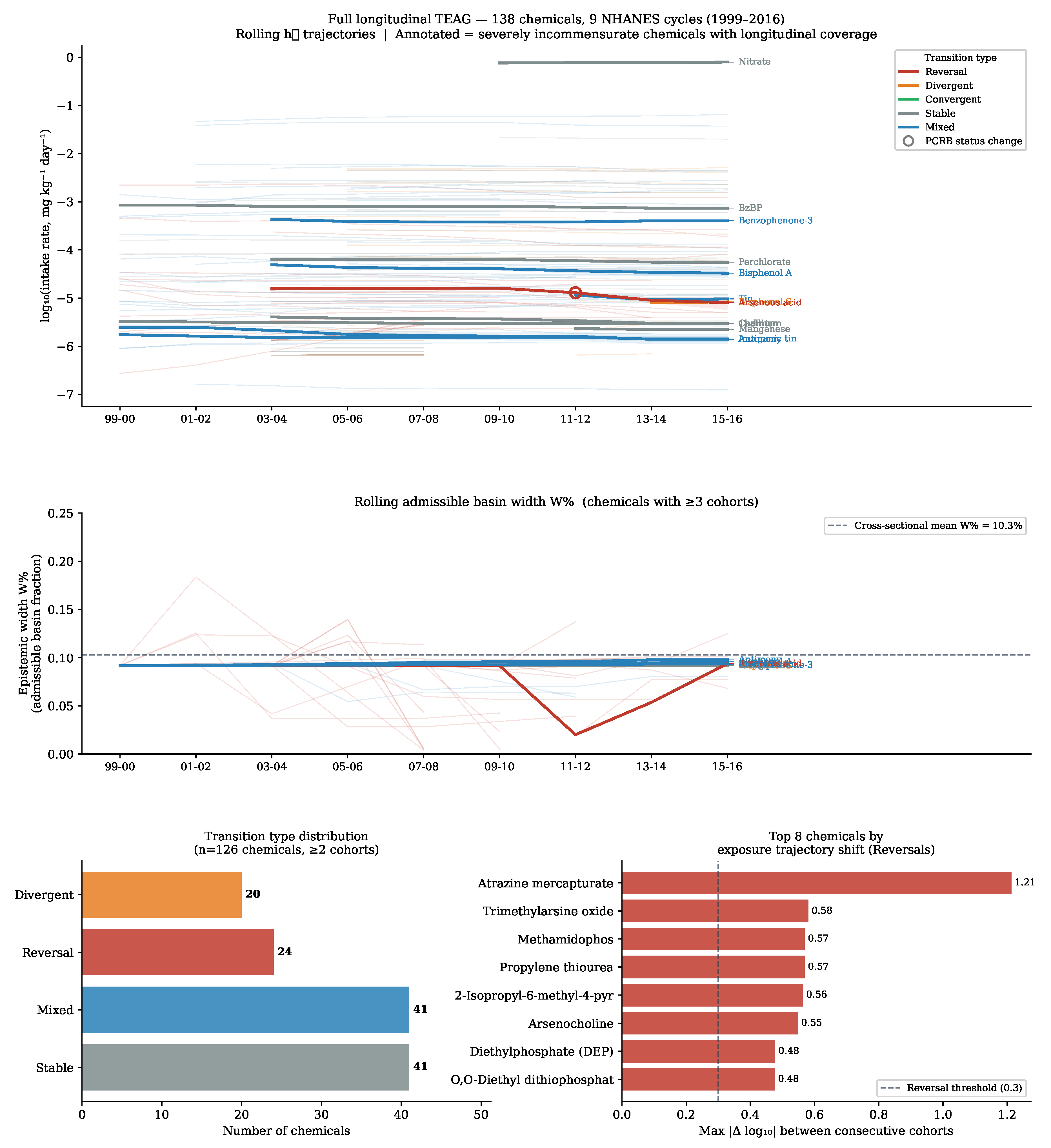
Bayesian inference treats each NHANES cohort as an independent posterior. TEAG can track the topology of the admissible basin across cohorts and detect qualitative changes in epistemic geometry — specifically, when a chemical transitions from PCRB-protected to the active falsification zone, or when the committed estimate shifts by more than log10 between consecutive cohorts. We term such events epistemic phase transitions. A chemical is classified as a Reversal if its maximum consecutive-cohort shift log10; as Divergent if moves monotonically away from baseline; as Convergent if moves monotonically toward baseline; and as Stable or Mixed otherwise. The 0.30 threshold corresponds to a 2-fold change in linear intake rate and is the same threshold shown in the figure caption’s reversal reference line.
Using the NHANES chemical-to-file mapping from Stanfield et al. (2022) Supplementary Table S1, we downloaded urinary concentration measurements for 138 chemicals directly from the CDC NHANES server across all available cycles (1999–2000 through 2015–2016). For each (chemical, cohort, demographic group) combination, group-level geometric means were computed using survey-weighted estimation, then converted to log10 intake rates via steady-state reverse dosimetry. TEAG geometry was applied using a rolling window: after each cohort t, the possibility distribution is built from the sequence of total-population log10-median estimates seen so far, , treating cohorts as observations. This encodes the epistemic question: what intake rates are consistent with the full longitudinal record?
Among the 138 chemicals with longitudinal data, transition types are: Reversal (24, 17%), Stable (41, 30%), Mixed (41, 30%), and Divergent (20, 14%), based on 126 chemicals with ≥2 cohorts. Twenty PCRB status changes occur across the full dataset — 20 chemicals with 1 flip each, and 2 chemicals with 2 flips. The dominant pattern is non-stability: 70% of chemicals show some form of geometric regime change as longitudinal evidence accumulates, a result that Bayesian cohort-by-cohort comparison cannot produce because it has no notion of epistemic regime.
The largest reversal is Atrazine mercapturate (DTXSID90160763), a herbicide metabolite, with log10 across only 3 cohorts, ending in the active falsification zone (). This represents a 16-fold shift in committed intake estimate and warrants immediate follow-up given atrazine’s status as a candidate for EPA regulatory action. Among the severely incommensurate chemicals with longitudinal coverage, Arsenous acid (DTXSID7074828, inorganic arsenic speciation) undergoes the most structurally significant transition: a log10 reversal between the 2013–2014 and 2015–2016 cohorts, accompanied by a PCRB status change from protected to active falsification beginning in the 2011–2012 cohort. This is the only severely incommensurate chemical in the longitudinal dataset whose epistemic commitment has moved outside the PCRB-protected zone, suggesting that the child-elder incommensurability for arsenous acid may be further destabilizing as cohort evidence accumulates.
Inorganic tin (DTXSID8052481), the chemical with the lowest in the entire dataset (), shows a stable longitudinal trajectory across all 9 NHANES cycles from 1999–2000 to 2015–2016, with drifting monotonically from to log10 and remaining PCRB-protected throughout. The stability of the longitudinal geometry contrasts sharply with its severe incommensurability: tin’s child-elder incommensurability is not an artifact of a single cohort but a persistent geometric feature of the 16-year exposure record. This makes tin the most robust and policy-relevant incommensurability finding in the dataset.
Figure 4.
Full longitudinal TEAG analysis across 138 chemicals and 9 NHANES cycles (1999–2016), constructed from raw NHANES XPT files. Top: rolling trajectories. Background lines (thin, semi-transparent) colored by transition type; bold labeled lines are the 13 severely incommensurate chemicals () with longitudinal NHANES coverage. Open circles mark PCRB status changes. Middle: rolling epistemic width across cohorts (chemicals with ≥3 cohorts; y-axis capped at 25%). Horizontal reference at cross-sectional mean . Bottom left: chemical counts by transition type ( chemicals with ≥2 cohorts). Bottom right: top 8 chemicals by maximum consecutive-cohort shift (all are Reversals).
Figure 4.
Full longitudinal TEAG analysis across 138 chemicals and 9 NHANES cycles (1999–2016), constructed from raw NHANES XPT files. Top: rolling trajectories. Background lines (thin, semi-transparent) colored by transition type; bold labeled lines are the 13 severely incommensurate chemicals () with longitudinal NHANES coverage. Open circles mark PCRB status changes. Middle: rolling epistemic width across cohorts (chemicals with ≥3 cohorts; y-axis capped at 25%). Horizontal reference at cross-sectional mean . Bottom left: chemical counts by transition type ( chemicals with ≥2 cohorts). Bottom right: top 8 chemicals by maximum consecutive-cohort shift (all are Reversals).
6.2. Epistemic Network Centrality
The coefficient defines a pairwise similarity metric over all 179 population-level possibility distributions. The full matrix, computed on a shared 5,000-point grid, produces a weighted epistemic network in which chemicals are nodes and edge weight is their pairwise .
Figure 5.
Epistemic network of 179 chemicals. Left: network graph with edges at (top 500 edges shown; overall mean ). Node size proportional to mean (epistemic centrality); color by chemical class. Key nodes labeled by chemical name; two isolated heterocyclic amines remain as DTXSIDs in the figure (DTXSID5020657 = Glu-P-1; DTXSID4020745 = IQ) as they are absent from the primary name map. Right: scatter of mean vs. log10, colored by chemical class. The 24 severely incommensurate chemicals are marked with a distinct symbol.
Figure 5.
Epistemic network of 179 chemicals. Left: network graph with edges at (top 500 edges shown; overall mean ). Node size proportional to mean (epistemic centrality); color by chemical class. Key nodes labeled by chemical name; two isolated heterocyclic amines remain as DTXSIDs in the figure (DTXSID5020657 = Glu-P-1; DTXSID4020745 = IQ) as they are absent from the primary name map. Right: scatter of mean vs. log10, colored by chemical class. The 24 severely incommensurate chemicals are marked with a distinct symbol.
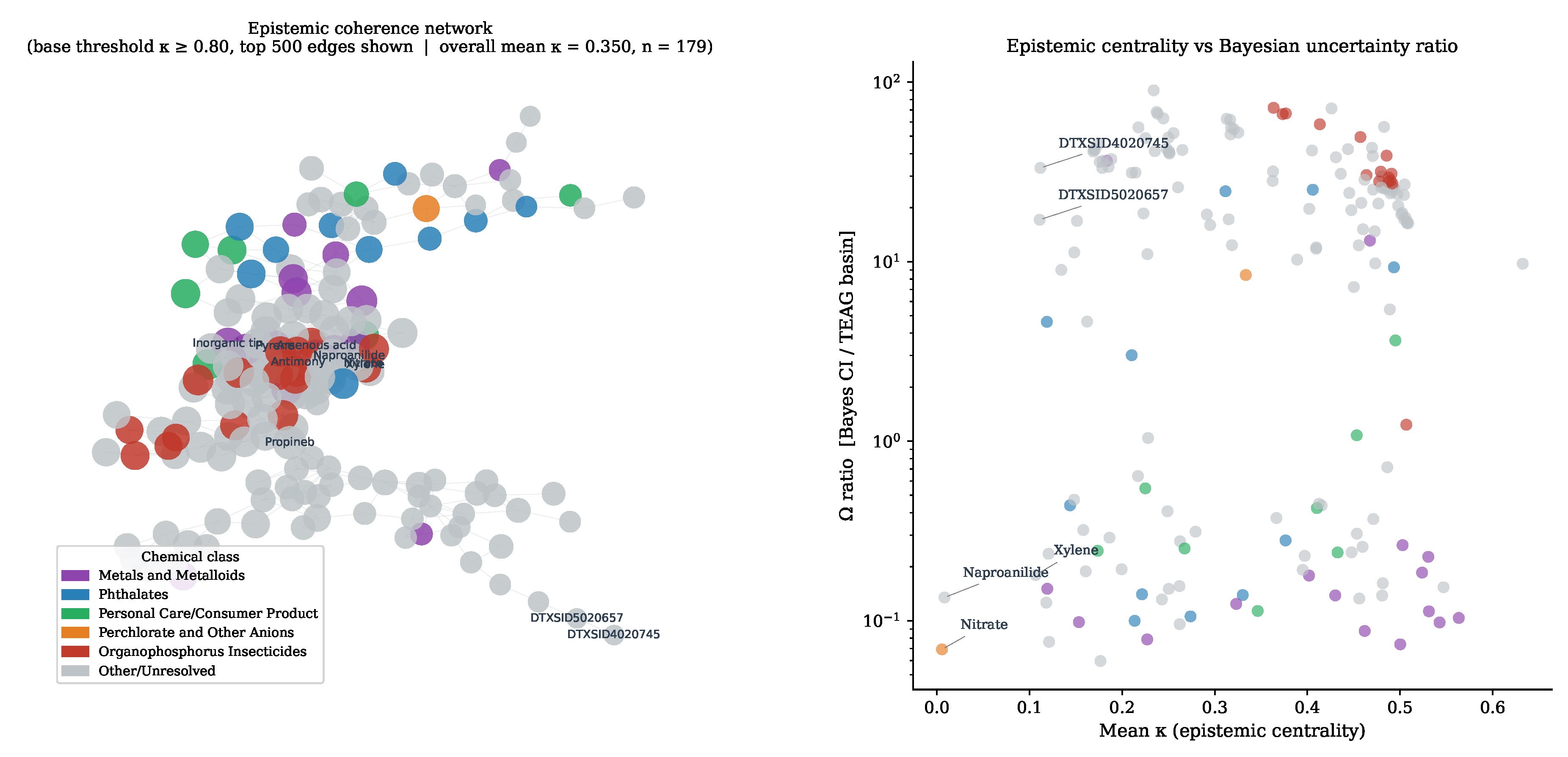
Mean across all pairs ranges from 0.006 to 0.632 (mean 0.350), confirming genuine spread across the network. On average each chemical has with 108 of the other 178 chemicals, indicating that the NHANES chemical landscape is highly heterogeneous in epistemic space.
The five most epistemically central chemicals — those whose committed exposure estimates are most consistent with the broadest cross-section of the dataset — are an unnamed sulfonyl urea herbicide (DTXSID1052741), inorganic tin (DTXSID8052481), tungsten (DTXSID7074828), molybdenum (DTXSID3024289), and a volatile organic compound (DTXSID5023879). Notably, three of the five most central chemicals are also among the 24 severely incommensurate chemicals (tin, tungsten, molybdenum). This is not a contradiction: a chemical can be epistemically central to the population-level distribution while being severely incommensurate across age groups, because centrality is defined over the population-level (which aggregates all groups) while incommensurability is defined over single-group distributions.
The two most epistemically isolated chemicals (DTXSID5024217, mean ; DTXSID8058118, mean ) have exposure estimates so far from any other chemical in the dataset that forward exposure models like SEEM are unlikely to extrapolate well to them. These are the highest-priority chemicals for targeted biomonitoring — not because their BER is necessarily low, but because their epistemic isolation means no surrogate inference from structurally similar chemicals is available.
6.3. Monitoring Urgency Score
We define a monitoring urgency score that identifies the chemicals where the next NHANES cohort is most likely to produce an epistemic surprise:
where is the Choquet surprisal (data tension), is the maximum epistemic distance of any demographic group from the committed estimate, and if the chemical is already in the active falsification zone, otherwise. is normalized to .
Figure 6.
Monitoring urgency score . Left: top 30 chemicals by , colored by ADF status. Incommensurability level labeled where available. Right: vs. child-specific urgency for the 69 chemicals with child data. Chemicals above the diagonal are more urgent for child monitoring than population-level monitoring. Color by incommensurability level.
Figure 6.
Monitoring urgency score . Left: top 30 chemicals by , colored by ADF status. Incommensurability level labeled where available. Right: vs. child-specific urgency for the 69 chemicals with child data. Chemicals above the diagonal are more urgent for child monitoring than population-level monitoring. Color by incommensurability level.
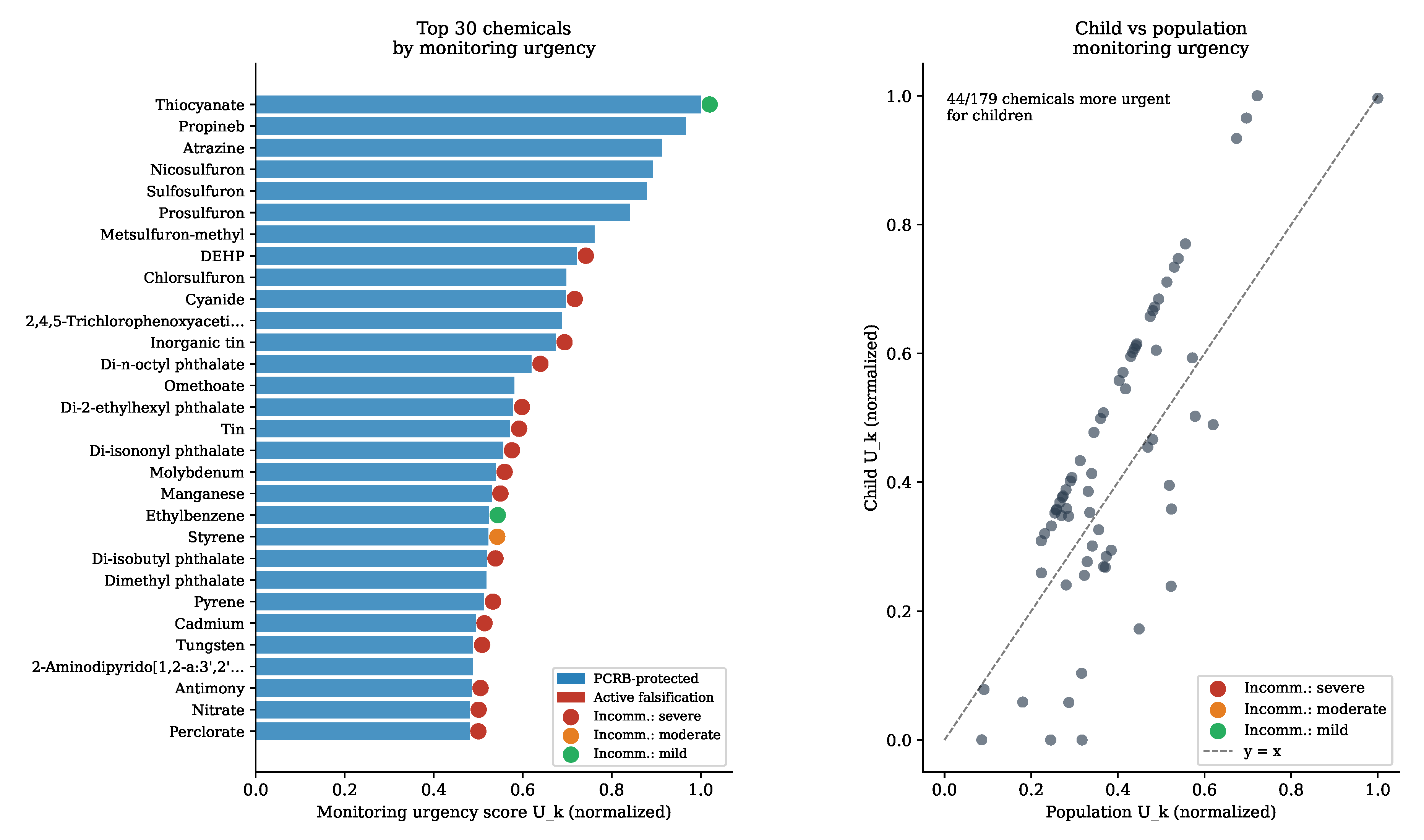
The top-20 chemicals by and the top-20 by share zero chemicals in common. This is the key validation result: captures prospective geometric risk (where new data is most likely to force revision) while captures retrospective width discrepancy (where Bayesian and TEAG differ most in spread). They are measuring different things, as intended.
DEHP ranks 8th overall by (0.722) but 1st by child-specific urgency (1.000), meaning it is the single chemical where the next NHANES cohort is most likely to produce a geometric surprise specifically for young children. Cyanide (DTXSID3020205) ranks 10th overall and 3rd for children. Together, the top-10 by include 8 of the 24 severely incommensurate chemicals, suggesting that incommensurability and prospective monitoring urgency are strongly co-occurring. A threshold between children and elderly, combined with high , is a natural joint criterion for triggering a child-specific regulatory review at the next NHANES release.
6.4. Incommensurability Transitivity
In classical probability, demographic similarity is transitive: if group A is similar to group B and group B is similar to group C, then A is similar to C. In possibility theory, the coefficient violates the triangle inequality. We define the transitivity gap:
for child group i (ages 3–5), elder group j (ages 66+), and intermediate group . A positive means the child-elder pair is more similar than expected from the intermediate chain (non-monotone, U-shaped gradient); negative means the gap is worse than the intermediate chain predicts (accelerating gradient).
Figure 7.
Incommensurability transitivity gaps for the 69 chemicals with both child and elder data. Left: heatmap of by chemical (y-axis, sorted by mean ) and intermediate group (x-axis). Red = positive (U-shaped), blue = negative (accelerating), white = near-transitive. Top 30 chemicals shown. Right: chemical counts by transitivity pattern, colored by incommensurability level.
Figure 7.
Incommensurability transitivity gaps for the 69 chemicals with both child and elder data. Left: heatmap of by chemical (y-axis, sorted by mean ) and intermediate group (x-axis). Red = positive (U-shaped), blue = negative (accelerating), white = near-transitive. Top 30 chemicals shown. Right: chemical counts by transitivity pattern, colored by incommensurability level.
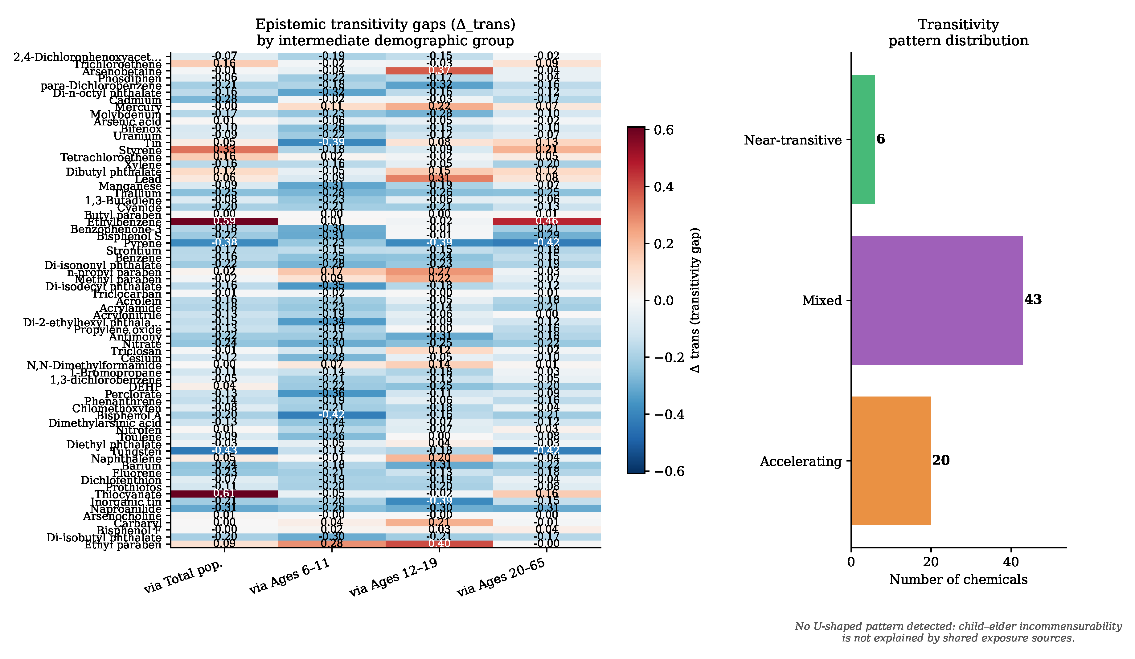
Among the 69 chemicals with data for both age extremes, the transitivity pattern distribution is: Mixed (43, 62%), Accelerating (20, 29%), Near-transitive (6, 9%), and U-shaped (0, 0%). The complete absence of U-shaped chemicals is itself a finding: the child-elder incommensurability in this dataset is never attributable to a shared elevated exposure source that simultaneously affects both very young and very old adults while bypassing middle-age groups. Instead, the dominant pattern is either accelerating (the child-elder gap is even worse than the intermediate groups suggest, meaning exposure declines monotonically and steeply with age) or mixed (the gradient is non-monotone but not uniformly so across all intermediate groups).
The 20 accelerating chemicals are disproportionately severe cases: the top-5 by mean include molybdenum (DTXSID3024289, ), an unresolved chemical (DTXSID8058118, ), tungsten (DTXSID7074828, ), and two additional severely incommensurate chemicals. For accelerating chemicals, the intermediate age groups are not adequate proxies for the child-elder gap: a regulatory standard calibrated on 12–19-year-olds will systematically underestimate how different the 3–5-year exposure profile is from the 66+ profile. This is a structural argument against using a single intermediate reference population to set standards intended to protect both extremes.
7. Regulatory Implications: Population-Differentiated Standards
7.1. The Geometric Argument for Differentiated Standards
Definition 2.12 establishes the mathematical condition: severe incommensurability () means that no single hypothesis achieves a possibility of 0.5 or greater for both demographic groups simultaneously. In the language of exposure science, this means that any single regulatory reference dose that is epistemically grounded for children — i.e., that falls within the region where children’s exposure distribution achieves — cannot simultaneously achieve the same epistemic grounding for elderly adults. The converse also holds. This is not a statement about statistical significance; it is a geometric statement about the incompatibility of the two populations’ epistemic states.
This matters for regulation in the following precise sense. Regulatory exposure limits (reference doses, tolerable daily intakes, maximum residue levels) are set at levels intended to be protective across the populations they cover. When two populations are epistemically incommensurate, any single limit is by construction set in a region where at least one population’s possibility distribution achieves less than 50% feasibility. The limit is either insufficiently protective for the high-exposure group (set too high) or unnecessarily restrictive for the low-exposure group (set too low).
7.2. The 24 Severely Incommensurate Chemicals
Table 3 presents the 24 chemicals with , ordered by ascending (most severely incommensurate first).
The pattern in Table 3 is chemically informative. The six chemicals with identical — the minimum in the dataset — are a heterogeneous group: two trace metals (tin, antimony), one transition metal (molybdenum), a heavy metal congener (tungsten), a volatile cyanogenic compound (cyanide), and a high-molecular-weight phthalate (DNOP). The shared value reflects a geometric coincidence: each of these chemicals has a 3–5-year group estimate that is well separated from the 66+ estimate relative to the bandwidth of their respective possibility distributions. The phthalates (DEHP, DIBP, DBP, BzBP) cluster in the range 0.28–0.33, consistent with their shared exposure pathways through plastic products and dust.
External validation from TRI and UCMR3. Cross-referencing the 24 severely incommensurate chemicals against EPA’s Toxics Release Inventory (TRI) and the Unregulated Contaminant Monitoring Rule cycle 3 (UCMR3, 2013–2015) provides independent evidence that the incommensurability is not a geometric artifact but reflects traceable environmental exposure pathways.
Five of the 24 severely incommensurate chemicals — Bisphenol A, Thallium, Cadmium, Manganese, and Antimony — are industrial reporters in TRI, meaning their demographic disparities in biomonitored concentrations align with known point-source industrial emissions. Of these, Cadmium is classified by TRI as both a carcinogen and a metal, and Lead (moderately incommensurate, ) is flagged as a persistent bioaccumulative toxic (PBT) in addition to being a carcinogen. The co-occurrence of industrial TRI reporting with severe epistemic incommensurability is consistent with the hypothesis that geographic proximity to TRI-reporting facilities is a structural driver of the child-elder divergence — children living near industrial point sources accumulate higher body burdens than their mobility-limited elderly counterparts for whom exposure pathways have shifted toward residential and dietary routes.
Two severely incommensurate chemicals appear in UCMR3 drinking water monitoring data, providing an independent ambient-exposure anchor. UCMR3 detection rates are reported at the public water system (PWS) level; population-level exposure prevalence requires weighting by the population served by each system, which is beyond the scope of this analysis. The rates below should be interpreted as the fraction of monitored PWSs with at least one detection above the minimum reporting level (MRL), not as the fraction of the U.S. population exposed at detectable levels.
Manganese (, also a TRI reporter) was detected in 59.8% of 5,935 PWSs monitored, with a median concentration of 5.5 g/L and a 95th-percentile value of 115.4 g/L — exceeding EPA’s health advisory level of 100 g/L. The NHANES urine manganese disparities across demographic groups are consistent with differential access to high-manganese water supplies, not solely biological variability in metabolism. Molybdenum ( — the second-lowest in the entire 138-chemical longitudinal dataset and among the lowest in the full 179-chemical cross-section) was detected in 40.3% of 62,986 PWSs monitored, with a median of 2.4 g/L. With a value that low, molybdenum is epistemically incommensurate across essentially all demographic groups in NHANES, and its presence in two of every five monitored public water systems provides a plausible mechanistic explanation: molybdenum intake from drinking water is age-invariant per unit volume consumed, but children consume proportionally more water per unit body weight and have lower elimination efficiency, producing the child-elder exposure divergence the TEAG geometry captures. Together, the UCMR3 results suggest that for at least two of the most severely incommensurate chemicals, population-differentiated standards could be anchored to ambient drinking water measurements rather than requiring individual biomonitoring.
7.3. Specific Regulatory Recommendations
Based on the TEAG incommensurability analysis, we make the following specific recommendations:
DEHP. The existing CPSC permanent ban on DEHP in children’s toys (above 0.1% concentration) acknowledges the differential exposure of children but does not translate to a child-specific reference dose. The TEAG result (, 9.4× child-to-elder fold) provides geometric justification for the EPA and CPSC to establish separate tolerable daily intake values for children under 6 and for adults aged 65 and older. The current EPA RfD of mg kg−1 day−1 is set for the general population; children aged 3–5 in NHANES 2015–2016 are already at 72% of this value from aggregate pathways.
Inorganic tin. With — the most severely incommensurate chemical in the dataset — inorganic tin presents the strongest geometric case for a child-specific standard. No child-specific regulatory limit currently exists in the United States for dietary tin. We recommend that FDA initiate a risk assessment process for age-differentiated tin exposure limits, with particular attention to the 3–5 year age group, dust ingestion as an exposure pathway, and tin-lined food cans as a primary source.
Phthalate class. DEHP, DNOP, DIBP, DBP, and BzBP are all severely incommensurate. All five are subject to CPSC restrictions in children’s products but without age-stratified reference doses. A class-level reassessment using population-stratified biomonitoring data is warranted.
Trace metals. Tungsten and molybdenum have no current U.S. regulatory reference doses in the context of environmental exposure (they are regulated industrially but not as environmental chemicals for the general public). The TEAG finding of severe incommensurability at for both, with child-to-elder folds of 7.4× and 6.9× respectively, constitutes a geometric argument for initiating formal risk assessment processes. For molybdenum in particular, the UCMR3 finding that 40.3% of U.S. public water systems detect it — with a median of 2.4 g/L across more than 62,000 systems — provides a specific regulatory entry point: EPA’s UCMR process exists precisely to assess whether unregulated contaminants warrant a national primary drinking water regulation. Molybdenum’s combination of near-universal drinking water presence and the most extreme demographic incommensurability in the dataset makes it the highest-priority candidate for UCMR-to-NPDWR regulatory escalation. Manganese, also detected by UCMR3 at 59.8% of public water systems with P95 = 115.4 g/L (exceeding EPA’s 100 g/L health advisory), and flagged as a TRI-reporting chemical, warrants parallel action.
General principle. For any chemical with between children and elderly adults in future NHANES biomonitoring cycles, we propose that population-differentiated reference doses be the default regulatory starting point rather than the exception. The geometric test is computationally trivial once the biomonitoring data are in hand.
8. Discussion
8.1. What TEAG Adds to Bayesian Biomonitoring
The results establish three categories of TEAG contribution that are inaccessible to Bayesian inference regardless of computational power or model complexity. More precisely, each contribution depends on geometric structure that no function of Bayesian posterior summary statistics can reproduce — a claim made precise by Proposition 2.14 for the incommensurability result and by construction for the falsification ordering and the separation of uncertainty sources.
Geometric separation of uncertainty sources. The Bayesian posterior conflates LOD censoring, stoichiometric ambiguity, and population variability into a single distribution. TEAG encodes each source in a distinct geometric object: LOD censoring appears in the shape of near the boundary of the measurable range; stoichiometric ambiguity appears in the width of ; demographic variability appears as the spread of observations and drives the ADF span. The mechanistic regression in Section 4.7 quantifies this: LOD fraction and together explain of the variance in log10, with LOD fraction the dominant marginal term () and independent (). Crucially, TEAG basin width is uncorrelated with LOD fraction (Figure 2, bottom-right).
The mean compression of the TEAG basin relative to the Bayesian 95% credible interval should not be read as TEAG compressing or discarding uncertainty. It reflects the redistribution of uncertainty across geometric structures: measurement noise lives in the shape of , stoichiometric ambiguity lives in the width of , and demographic variability lives in the spread of the observations . The Bayesian CI integrates all of these into one interval; the TEAG basin encodes only the region of geometric commitment, with the remaining uncertainty traceable to its specific source. This redistribution enables targeted data collection decisions — more measurements to reduce LOD fraction, better metabolite mapping to reduce , finer demographic stratification — rather than generic uncertainty reduction.
Falsification ordering. Table 1 is a geometric object with no probabilistic analog. The falsification priority of a demographic group is its distance from the committed population-level estimate in the possibilistic geometry. Bayesian inference has no such ordering because the posterior integrates over all groups simultaneously; there is no notion of which group would first force revision of a population-level commitment. The Bayesian framework tells you that uncertainty exists; the falsification ordering tells you where the model is most exposed.
This distinction has direct operational consequences. The monitoring urgency score (Section 6.3) translates the falsification geometry into a prospective priority list for the next NHANES cohort. The zero overlap between the top-20 by and the top-20 by confirms that falsification priority and retrospective uncertainty width are geometrically independent — knowing that Bayesian uncertainty is wide for a chemical tells you nothing about whether that chemical is at the edge of epistemic commitment. For monitoring design, experiment prioritization, and adaptive sampling, this ordering is the actionable output; posterior widths are not.
Epistemic incommensurability. The coefficient (Definition 2.11) measures the maximum simultaneous feasibility of any hypothesis for two populations. It is not a Bayes factor (which requires a prior), not a p-value (which requires a null hypothesis), and not a Kullback–Leibler divergence (which requires the two distributions to be defined on the same support in the probabilistic sense). It is a geometry of epistemic overlap. Proposition 2.14 establishes formally that cannot be reproduced from any function of Bayesian posterior summary statistics; the proof constructs two chemicals with identical posterior means, variances, and credible interval widths that produce different values by construction. The qualifier “no function of posterior summaries” is the precise claim; whether other probabilistic representations beyond summary statistics could capture remains an open question, though we note that is a non-linear functional of the joint group-level data configuration that standard probabilistic models do not track.
TEAG as constraint-based rather than generative inference. A natural question is: where does the TEAG model come from, if not from a likelihood and prior? The answer is that TEAG is a constraint-based inference system, not a generative one, and this is a principled choice rather than a limitation. Bayesian inference is the right tool when a well-specified generative process can be assumed — when data arise from a known stochastic mechanism whose parameters one wishes to estimate. The NHANES biomonitoring problem does not have this structure: the mapping from chemical intake to urinary metabolite concentration involves unknown stoichiometric proportions, unknown route fractions, and unknown individual toxicokinetics. Stanfield et al. (2022) handle this honestly by propagating uncertainty through a suite of assumptions. TEAG handles it differently: rather than specifying a generative model and integrating over its uncertainty, it asks which intake rates are consistent with the available group-level summaries given the constraints that (i) each group’s estimate must be feasible, and (ii) the committed estimate must be geometrically central to the data cloud. These are constraints on admissibility, not assumptions about mechanism. The result is a committed estimate and a falsification geometry that makes no claim about how the data were generated — only about what the data permit. This is the right epistemic posture for a problem where the generative process is partially unknown.
8.2. Why Bayesian Inference Cannot Express Regulatory Incommensurability
The central result of this paper — that 24 chemicals are severely incommensurate across age groups — is not a result that Bayesian inference could have produced with more data, a better prior, or a more sophisticated model. The limitation is structural, not computational. Understanding why is important both for the paper’s argument and for the broader question of when possibilistic geometry adds something genuinely new.
Bayesian inference integrates over hypotheses. The posterior is a probability distribution over intake rates, obtained by weighting each hypothesis h by its likelihood and prior. The summary statistics that emerge — posterior mean, variance, credible interval — are all integrals over h with respect to this distribution. Crucially, when computing the posterior for a single demographic group, the analysis integrates over all hypotheses that are consistent with that group’s data; when comparing two groups, one computes the overlap between two such integrals.
The coefficient evaluates the intersection of two feasibility sets. Specifically, asks: is there any hypothesis that is simultaneously highly feasible for both group i and group j? The answer depends not on the marginal distributions of h under each group’s data, but on their joint structure — on which hypotheses lie in the intersection of their feasibility regions.
Integration destroys intersection structure. When the Bayesian posterior integrates over hypotheses for group i, it combines a region of high posterior mass (near the group-i mode) with regions of lower mass. The resulting distribution is spread across , and any hypothesis in the support of the posterior is “possible” in the probabilistic sense, to some positive probability. Two groups with non-overlapping modes but overlapping tails will produce posteriors that share support across much of even when the groups are epistemically very different. The Bayesian test for different means (a t-test or posterior difference) detects location shifts but not feasibility incompatibility.
By contrast, the coefficient directly evaluates the maximum simultaneous feasibility. If group i’s possibility distribution peaks at and group j’s peaks at , and if is large relative to the bandwidth b, then is small everywhere — small near because is small, and small near because is small. The supremum of this minimum is , and it can be very small even when both posteriors have broad support. This is precisely what severe incommensurability means: not just that the groups have different means, but that no single hypothesis is simultaneously consistent with both.
The practical implication is this: a Bayesian analysis of the NHANES data can tell you that children have significantly higher median inferred intake than elderly adults for tin ( by any reasonable test). TEAG tells you that the highest-feasibility intake rate for children achieves only 24.7% simultaneous feasibility for elderly adults — meaning that a regulatory standard set at the epistemically grounded level for children is, in the possibilistic sense, less than one-quarter as grounded for the elderly population. These are different claims. The first is about the direction and magnitude of a difference; the second is about whether a single regulatory standard can be grounded for both populations simultaneously. Only the second claim has direct regulatory implications for standard-setting, and only TEAG can make it.
8.3. Why Integration Destroys Overlap Structure
Here is the core intuition, stripped to its essentials.
Imagine two people standing in a large field. Person A is somewhere near the left side; Person B is somewhere near the right side. You want to know: is there any spot in the field where both people could be standing simultaneously?
The Bayesian answer describes each person’s location as a probability distribution — a blur of probability mass spread over the field, highest near where they are most likely to be, tapering off toward zero at the edges. To check for overlap, you look at whether the two blurs share any probability mass. Because all continuous distributions have positive density everywhere in their support, two people on opposite sides of a large field still have overlapping blurs. Any significance test based on these distributions can only tell you whether the means are different; it cannot tell you whether a specific spot is simultaneously consistent with both locations. The integration that produces the distributions has already lost that information.
The TEAG answer asks a sharper question: for each spot in the field, what is the minimum plausibility assigned by both Person A’s distribution and Person B’s distribution? The coefficient is the maximum of this minimum over all spots. If A is on the far left and B on the far right, then every spot near A has low plausibility for B, and every spot near B has low plausibility for A. The minimum is small everywhere, and is small. This is severe incommensurability: not just that A and B are far apart, but that no spot is simultaneously plausible for both.
The mathematical reason integration fails is that depends on the pointwise minimum of two functions, which is a non-linear operation. Integration — summing, averaging, marginalizing — is a linear operation. No linear combination of the two distributions can recover the pointwise minimum between them. You cannot integrate your way to an intersection.
Proposition 2.14 makes this precise: two chemicals can have identical posterior means, variances, and credible interval widths yet different values, because the group-level structure that determines is exactly what integration erases. The practical consequence is that Bayesian inference, however carefully specified, cannot ask the regulatory question at stake: not “are these groups different?” but “does any standard simultaneously serve both?” Only a framework that preserves the intersection structure of feasibility regions can answer that question. TEAG does. Integration does not.
8.4. Relationship to the Broader Exposure Science Literature
The finding that children have higher inferred exposure to most chemicals is consistent with and corroborated by Stanfield et al. (2022), who show children aged 3–5 have higher estimated intake than the total population for 61 of 69 chemicals with data for that age group. Wambaugh et al. (2014) established this pattern for children aged 6–11; Stanfield et al. (2022) extends it to the youngest cohort.
What TEAG adds is not the direction of the difference but its geometric character. The Bayesian finding is “children have higher median estimated exposure, and the 95% CI does not overlap for some chemicals.” The TEAG finding is “children and elderly adults occupy epistemically separate regions of hypothesis space for 24 chemicals, and this separation is geometrically sufficient to preclude a common regulatory standard.” These are not the same claim. The second requires no significance test and is not subject to multiple-comparison corrections; it is a statement about the structure of the possibility distributions.
The SEEM consensus exposure model (Ring et al., 2019), which Stanfield et al. (2022) evaluate against their Bayesian estimates, shows poor correlation () for most chemical classes not in its calibration set. The TEAG ADF analysis provides a complementary diagnostic: the 48 chemicals in the active falsification zone are those for which new data is most likely to produce large revisions, making them natural priorities for SEEM recalibration.
8.5. Limitations
The TEAG analysis inherits the data limitations of the bayesmarker pipeline. The group-level estimates are Bayesian posterior medians, not raw observations; any systematic biases in the Bayesian inference (e.g., from the steady-state assumption, LOD handling, or metabolite mapping) propagate into the possibilistic geometry. The steady-state assumption of Stanfield et al. (2022) is acknowledged by the authors as a limitation for chemicals with very short half-lives or highly episodic exposure patterns; the TEAG analysis does not resolve this.
The bandwidth log10 is a default choice that affects the shape of and therefore the ADF span and admissible basin width. Table 4 reports the sensitivity of the key incommensurability findings to bandwidth across the range log10.
The 24 severely incommensurate chemicals are stable across . At (the widest bandwidth considered, more than twice the inter-group spacing for most chemicals), 18 of 24 remain severely incommensurate; the 6 that cross the threshold do so marginally ( in the range 0.50–0.57), and none approach commensurability. The qualitative conclusions of Section 7 are robust.
The population-differentiated regulatory standards called for in Section 7 require additional toxicokinetic and hazard characterization work beyond what biomonitoring data alone can provide. The TEAG incommensurability result identifies which chemicals warrant such work; it does not itself constitute a full risk assessment.
8.6. Future Directions
The possibilistic geometry introduced here generalizes naturally to multivariate hypothesis spaces (joint estimation of intake rates across multiple chemicals) via the MVEE framework of Jah (2026). Applied to cumulative exposure assessment — a growing priority in exposure science (Bopp et al., 2018) — a multivariate coefficient would identify chemical combinations for which demographic-differentiated standards are needed. This is a natural extension for the TEAG/NHANES framework.
The epistemic phase transition framework of Section 6.1 demonstrates that 70% of 138 chemicals with longitudinal NHANES coverage show geometric regime changes across up to 9 cohorts (1999–2016) — a result inaccessible to Bayesian cohort comparison. The current analysis uses total-population geometric means derived from raw NHANES XPT files via simplified reverse dosimetry; the natural next step is to replace these with the full 11-group per-cohort bayesmarker output, which would enable the complete demographic-stratified longitudinal geometry for all 138 chemicals. Making the full per-cohort bayesmarker output available as a structured CSV — a modest addition to the existing open-source package — would immediately enable this. NHANES 2017–2018 and 2019–2020 data are now publicly available and would allow the first prospective test of whether the monitoring urgency scores computed at 2015–2016 correctly predict which chemicals produce epistemic phase transitions in subsequent cycles.
9. Conclusion
We have demonstrated that possibilistic geometry, formalized through TEAG, recovers the point estimates of Bayesian biomonitoring inference with high fidelity () while surfacing geometric structure that is inaccessible to any probabilistic method. The admissible epistemic basin is on average narrower than the Bayesian credible interval because it geometrically separates uncertainty sources rather than aggregating them. The falsification ordering of demographic groups, the Choquet data tension scalar, and the ADF geometry provide a monitoring infrastructure with no probabilistic analog.
The regulatory incommensurability result is the most consequential finding. All 69 chemicals for which both children aged 3–5 and adults aged 66 and older have NHANES biomonitoring data are epistemically incommensurate in the possibilistic sense. For 24 of these chemicals — including DEHP, inorganic tin, tungsten, molybdenum, antimony, cyanide, DNOP, DIBP, DBP, and BzBP — the incommensurability is severe enough that no single regulatory exposure standard can be simultaneously epistemically grounded for both populations. We call explicitly for population-differentiated reference doses for these 24 chemicals, with particular urgency for DEHP and inorganic tin, and propose that in NHANES biomonitoring data be adopted as a standing geometric criterion for triggering age-stratified regulatory review.
The methods are implemented in open, reproducible code; the underlying NHANES data are publicly available from the CDC; and the TEAG geometry is fully specified in the definitions and propositions of Section 2. The result is a framework that any exposure scientist or risk analyst can apply to any future biomonitoring dataset.
Supplementary Materials
The following supporting information can be downloaded at the website of this paper posted on Preprints.org.
Data Availability Statement
All input data used in this analysis are publicly available. NHANES urine biomonitoring data: https://wwwn.cdc.gov/nchs/nhanes/. EPA Toxics Release Inventory data: https://www.epa.gov/toxics-release-inventory-tri-program. EPA UCMR3 occurrence data: https://www.epa.gov/dwucmr/occurrence-data-unregulated-contaminant-monitoring-rule. The bayesmarker R package and its input data: https://github.com/USEPA/CompTox-HumanExposure-bayesmarker. The TEAG framework is proprietary; implementation details are not publicly available.
Acknowledgments
The author thanks the Jah Decision Intelligence Group at The University of Texas at Austin for computational support, and acknowledges the foundational work of Stanfield et al. (2022) and the EPA bayesmarker team whose open-source pipeline and publicly released data made this comparative analysis possible. The NHANES biomonitoring data are collected and maintained by the U.S. Centers for Disease Control and Prevention and are freely available at https://wwwn.cdc.gov/nchs/nhanes/. This work was supported in part by GaiaVerse, Ltd.
Conflicts of Interest
The author declares no competing interests.
References
- Bopp, S. K.; Barouki, R.; Brack, W.; Dalla Costa, S.; Dorne, J.-L. C.; Drakvik, P. E.; Faust, M.; Karjalainen, T. K.; Kolar, B.; Kortenkamp, A.; et al. Current EU research activities on combined exposures to multiple chemical and non-chemical stressors: a synopsis of four European research projects. Environment International 2018, 120, 544–562. [Google Scholar] [CrossRef] [PubMed]
- Cramér, H. Mathematical Methods of Statistics; Princeton University Press, 1946. [Google Scholar]
- Centers for Disease Control and Prevention. National Health and Nutrition Examination Survey; National Center for Health Statistics, 2023; Available online: https://wwwn.cdc.gov/nchs/nhanes/.
- U.S. Environmental Protection Agency. Toxics Release Inventory (TRI) Basic Plus Data Files. 2015. Available online: https://www.epa.gov/toxics-release-inventory-tri-program/tri-basic-plus-data-files-calendar-years-1987-2022.
- U.S. Environmental Protection Agency. Third Unregulated Contaminant Monitoring Rule (UCMR3) Occurrence Data, 2013–2015. 2016. Available online: https://www.epa.gov/dwucmr/occurrence-data-unregulated-contaminant-monitoring-rule.
- Dubois, D.; Prade, H. Possibility theory and its applications: Where do we stand? In Springer Handbook of Computational Intelligence; Kacprzyk, J., Pedrycz, W., Eds.; Springer, 2015; pp. 31–60. [Google Scholar]
- Dubois, D.; Prade, H. Possibility Theory; Plenum Press, 1988. [Google Scholar]
- U.S. Environmental Protection Agency. IRIS Assessment for Di(2-ethylhexyl) Phthalate (DEHP), CASRN 117-81-7. Integrated Risk Information System. Available online: https://iris.epa.gov/ChemicalLanding/&substance_nmbr=14.
- U.S. Food and Drug Administration. Guidance for Industry: Action Levels for Poisonous or Deleterious Substances in Human Food and Animal Feed; Silver Spring, 2022; Available online: https://www.fda.gov/food/guidance-documents-regulatory-information-topic-food-and-dietary-supplements.
- Consumer Product Safety Improvement Act of 2008. Pub. L. No. 110-314.
- Jah, M. K. The Epistemic State Propagation Framework: Possibilistic orbit determination with validated real-data performance. arXiv 2025, arXiv:2508.20806. [Google Scholar]
- Jah, M. K. Epistemic wavefronts and the tropical Hamilton–Jacobi geometry of knowing. Preprint, preprints.org. 2026.
- Lehmler, H. J.; Gadogbe, M.; Liu, B.; Bao, W. Environmental tin exposure in a nationally representative sample of U.S. adults and children: The National Health and Nutrition Examination Survey 2011–2014. Environmental Pollution 2018, 240, 599–606. [Google Scholar] [CrossRef] [PubMed]
- Litvinov, G. L.; Maslov, V. P. (Eds.) Idempotent Mathematics and Mathematical Physics; Contemporary Mathematics 377, AMS, 2005. [Google Scholar]
- Maslov, V. P. Idempotent Analysis; Advances in Soviet Mathematics 13; AMS, 1992; p. 13. [Google Scholar]
- Plummer, M. JAGS: A program for analysis of Bayesian graphical models using Gibbs sampling. In Proceedings of the 3rd International Workshop on Distributed Statistical Computing, Vienna, Austria; 2003. [Google Scholar]
- Rao, C. R. Information and the accuracy attainable in the estimation of statistical parameters. Bulletin of the Calcutta Mathematical Society 1945, 37, 81–91. [Google Scholar]
- Reyes, J. M.; Price, P. S. Temporal trends in exposures to six phthalates from biomonitoring data: implications for cumulative risk. Environmental Science & Technology 2018, 52, 12475–12483. [Google Scholar] [CrossRef]
- Ring, C. L.; Arnot, J.; Bennett, D. H.; Egeghy, P.; Fantke, P.; Huang, L.; et al. Consensus modeling of median chemical intake for the U.S. population based on predictions of exposure pathways. Environmental Science & Technology 2019, 53, 719–732. [Google Scholar]
- Stanfield, Z.; Setzer, R. W.; Hull, V.; Sayre, R. R.; Isaacs, K. K.; Wambaugh, J. F. Bayesian inference of chemical exposures from NHANES urine biomonitoring data. Journal of Exposure Science & Environmental Epidemiology 2022, 32, 833–846. [Google Scholar] [CrossRef]
- Wambaugh, J. F.; Setzer, R. W.; Reif, D. M.; Gangwal, S.; Mitchell-Blackwood, J.; Arnot, J. A.; et al. High-throughput models for exposure-based chemical prioritization in the ExpoCast project. Environmental Science & Technology 2013, 47, 8479–8488. [Google Scholar]
- Wambaugh, J. F.; Wang, A.; Dionisio, K. L.; Frame, A.; Egeghy, P.; Judson, R.; et al. High throughput heuristics for prioritizing human exposure to environmental chemicals. Environmental Science & Technology 2014, 48, 12760–12767. [Google Scholar] [CrossRef] [PubMed]
- Zadeh, L. A. Fuzzy sets as a basis for a theory of possibility. Fuzzy Sets and Systems 1978, 1, 3–28. [Google Scholar] [CrossRef]
Figure 1.
by chemical class, sorted by median ascending. Points are color-coded by incommensurability level: severe (, red), moderate (, amber), mild (, green). Vertical reference lines at (severe threshold) and . n per class shown on the right.
Figure 1.
by chemical class, sorted by median ascending. Points are color-coded by incommensurability level: severe (, red), moderate (, amber), mild (, green). Vertical reference lines at (severe threshold) and . n per class shown on the right.
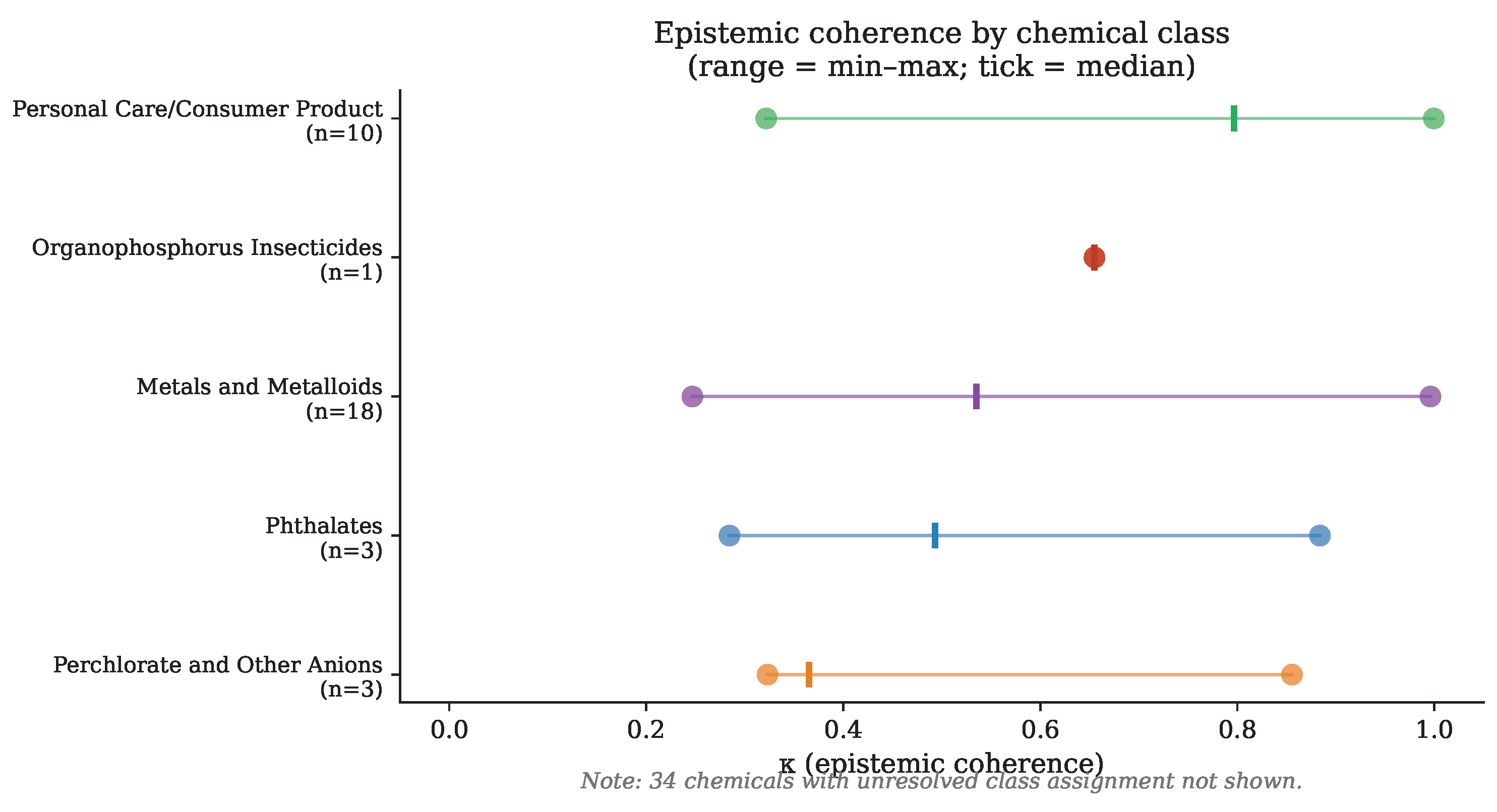
Figure 2.
Mechanistic decomposition of (Bayesian 95% CI width / TEAG admissible basin span) across all 179 chemicals. Four panels: (top-left) vs. fraction below LOD, colored by category (1 = blue, 2–3 = amber, ≥4 = red); (top-right) vs. with jitter, colored by LOD fraction quartile; (bottom-left) log10
(Bayesian CI width) vs. log10
(TEAG basin W%), 1:1 reference line shown; (bottom-right) TEAG W% vs. fraction below LOD, showing that TEAG basin width is insensitive to censoring. LOWESS smoothers throughout. ranges from 1 to 18 across all 179 chemicals; LOD fraction available for 60 chemicals. OLS on the 60 chemicals with both predictors yields .
Figure 2.
Mechanistic decomposition of (Bayesian 95% CI width / TEAG admissible basin span) across all 179 chemicals. Four panels: (top-left) vs. fraction below LOD, colored by category (1 = blue, 2–3 = amber, ≥4 = red); (top-right) vs. with jitter, colored by LOD fraction quartile; (bottom-left) log10
(Bayesian CI width) vs. log10
(TEAG basin W%), 1:1 reference line shown; (bottom-right) TEAG W% vs. fraction below LOD, showing that TEAG basin width is insensitive to censoring. LOWESS smoothers throughout. ranges from 1 to 18 across all 179 chemicals; LOD fraction available for 60 chemicals. OLS on the 60 chemicals with both predictors yields .
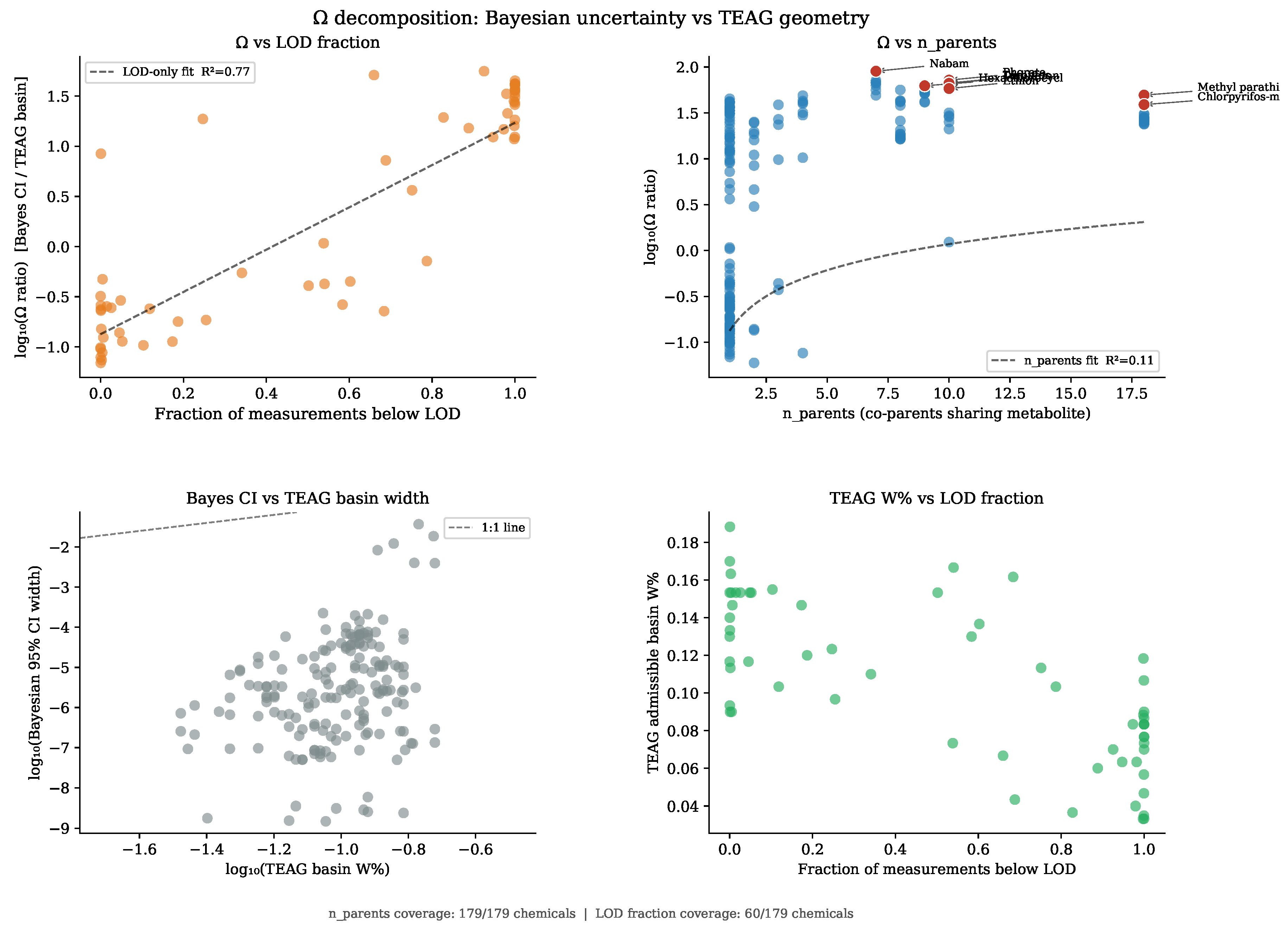
Figure 3.
Full TEAG possibilistic geometry for the two illustrative chemicals. Each panel shows: (filled gray curve, left axis); (solid line, right axis); (dashed, right axis); (bold blue, right axis); admissible basin (shaded band); (vertical dashed line); PCRB threshold (horizontal dashed line); ADF loci (tick marks); group observations as rug marks (children in red, elderly in blue, others in gray); Bayesian 95% CI bracket below the axis.
Figure 3.
Full TEAG possibilistic geometry for the two illustrative chemicals. Each panel shows: (filled gray curve, left axis); (solid line, right axis); (dashed, right axis); (bold blue, right axis); admissible basin (shaded band); (vertical dashed line); PCRB threshold (horizontal dashed line); ADF loci (tick marks); group observations as rug marks (children in red, elderly in blue, others in gray); Bayesian 95% CI bracket below the axis.
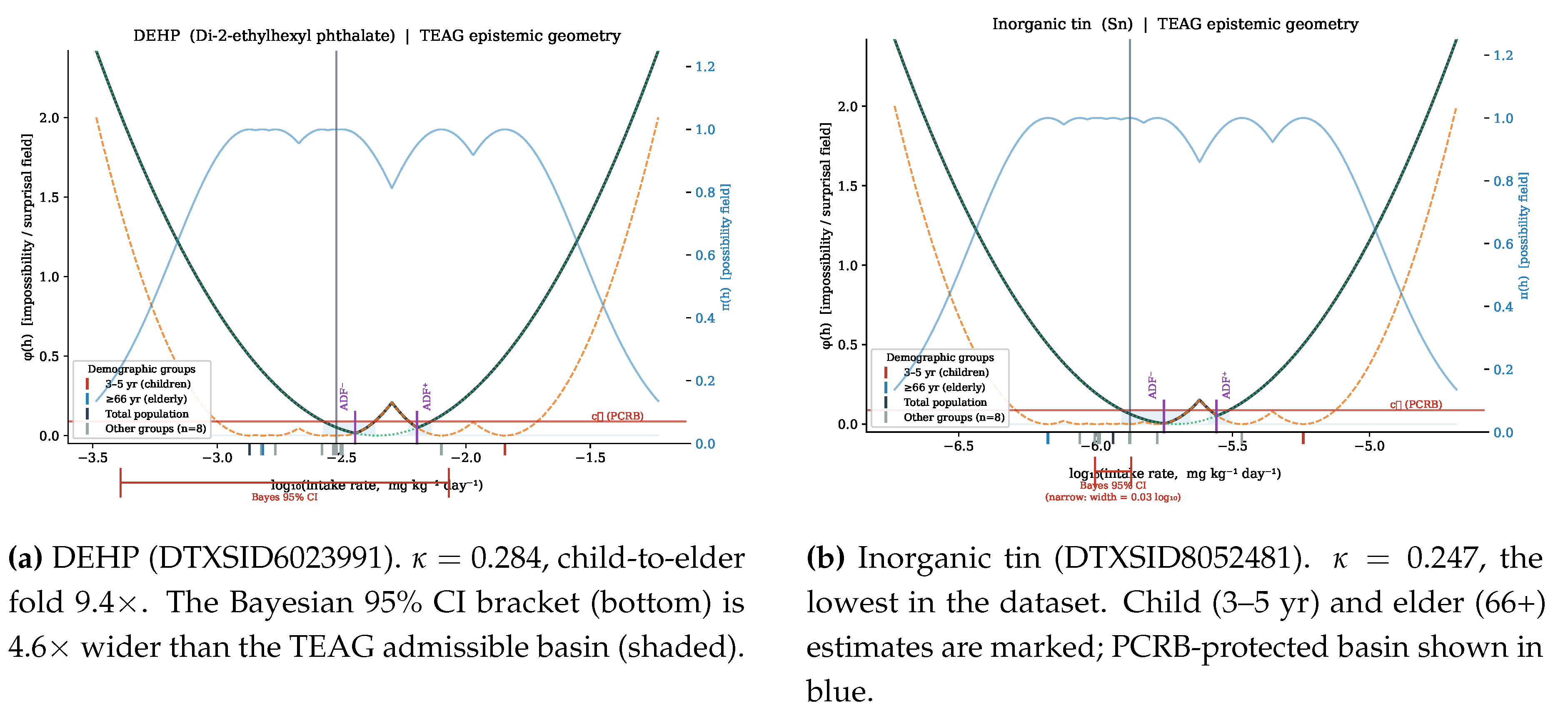

Table 1.
Epistemic vulnerability ranking of demographic groups. Mean distance is in log10
units over all chemicals with data for that group. Fold from medioid . No Bayesian analog exists for this ordering.
Table 1.
Epistemic vulnerability ranking of demographic groups. Mean distance is in log10
units over all chemicals with data for that group. Fold from medioid . No Bayesian analog exists for this ordering.
| Rank | Demographic group | n chem. | Mean dist. (log10) | Fold from |
| 1 | Ages 3–5 years | 69 | 0.275 | 1.89× |
| 2 | Ages 66 and older | 178 | 0.171 | 1.48× |
| 3 | BMI > 30 | 179 | 0.157 | 1.44× |
| 4 | Ages 6–11 years | 179 | 0.143 | 1.39× |
| 5 | Ages 12–19 years | 179 | 0.131 | 1.35× |
| 6 | Reproductive-age female | 179 | 0.122 | 1.32× |
| 7 | Ages 20–65 years | 179 | 0.121 | 1.32× |
| 8 | Female | 179 | 0.117 | 1.31× |
| 9 | Total population | 179 | 0.109 | 1.28× |
| 10 | Male | 179 | 0.103 | 1.27× |
| 11 | BMI ≤ 30 | 179 | 0.084 | 1.21× |
Table 2.
incommensurability summary by chemical class. Classes sorted by median ascending. “Other” contains 34 chemicals whose class could not be resolved from the CompTox API.
Table 2.
incommensurability summary by chemical class. Classes sorted by median ascending. “Other” contains 34 chemicals whose class could not be resolved from the CompTox API.
| Chemical class | n | Severe | Moderate | Mild | Median | % severe |
| Perchlorate & Other Anions | 3 | 2 | 0 | 1 | 0.365 | 67% |
| Phthalates | 3 | 2 | 0 | 1 | 0.493 | 67% |
| Metals & Metalloids | 18 | 9 | 4 | 5 | 0.535 | 50% |
| Other (unresolved) | 34 | 8 | 19 | 7 | 0.627 | 24% |
| Organophosphorus Insecticides | 1 | 0 | 1 | 0 | 0.655 | 0% |
| Personal Care/Consumer Prod. | 10 | 3 | 2 | 5 | 0.796 | 30% |
Table 3.
The 24 chemicals with severe epistemic incommensurability () between children aged 3–5 and adults aged 66 and older. Child intake is the TEAG-estimated log10
median for the 3–5 age group; elder intake is the corresponding value for the 66+ group. Fold = child/elder intake ratio in linear scale.
Table 3.
The 24 chemicals with severe epistemic incommensurability () between children aged 3–5 and adults aged 66 and older. Child intake is the TEAG-estimated log10
median for the 3–5 age group; elder intake is the corresponding value for the 66+ group. Fold = child/elder intake ratio in linear scale.
| Chemical | Child 3–5 | Elder 66+ | Fold | |
| (mg kg−1 d−1) | ||||
| Inorganic tin | 0.247 | 8.6× | ||
| Tungsten | 0.247 | 7.4× | ||
| Molybdenum | 0.247 | 6.9× | ||
| Cyanide | 0.247 | 8.0× | ||
| DNOP | 0.247 | 7.7× | ||
| Antimony | 0.247 | 8.2× | ||
| DEHP | 0.284 | 9.4× | ||
| DIBP | 0.322 | 5.6× | ||
| DBP | 0.323 | 5.6× | ||
| BzBP | 0.324 | 5.6× | ||
| [14 additional chemicals; full list in Supplementary Table S1] | ||||
Table 4.
Bandwidth sensitivity analysis. Counts of severely incommensurate chemicals (), total incommensurate chemicals (), and mean across the 69 chemicals with child and elder data, at five bandwidth values. The default used throughout is .
Table 4.
Bandwidth sensitivity analysis. Counts of severely incommensurate chemicals (), total incommensurate chemicals (), and mean across the 69 chemicals with child and elder data, at five bandwidth values. The default used throughout is .
| b (log10) | 0.15 | 0.20 | 0.25 | 0.30 | 0.40 |
| Severe () | 26 | 25 | 24 | 24 | 18 |
| Incommensurate () | 69 | 69 | 69 | 69 | 67 |
| Mean | 0.68 | 0.70 | 0.71 | 0.72 | 0.76 |
Disclaimer/Publisher’s Note: The statements, opinions and data contained in all publications are solely those of the individual author(s) and contributor(s) and not of MDPI and/or the editor(s). MDPI and/or the editor(s) disclaim responsibility for any injury to people or property resulting from any ideas, methods, instructions or products referred to in the content. |
© 2026 by the authors. Licensee MDPI, Basel, Switzerland. This article is an open access article distributed under the terms and conditions of the Creative Commons Attribution (CC BY) license (http://creativecommons.org/licenses/by/4.0/).
Copyright: This open access article is published under a Creative Commons CC BY 4.0 license, which permit the free download, distribution, and reuse, provided that the author and preprint are cited in any reuse.


