Submitted:
08 April 2026
Posted:
09 April 2026
You are already at the latest version
Abstract
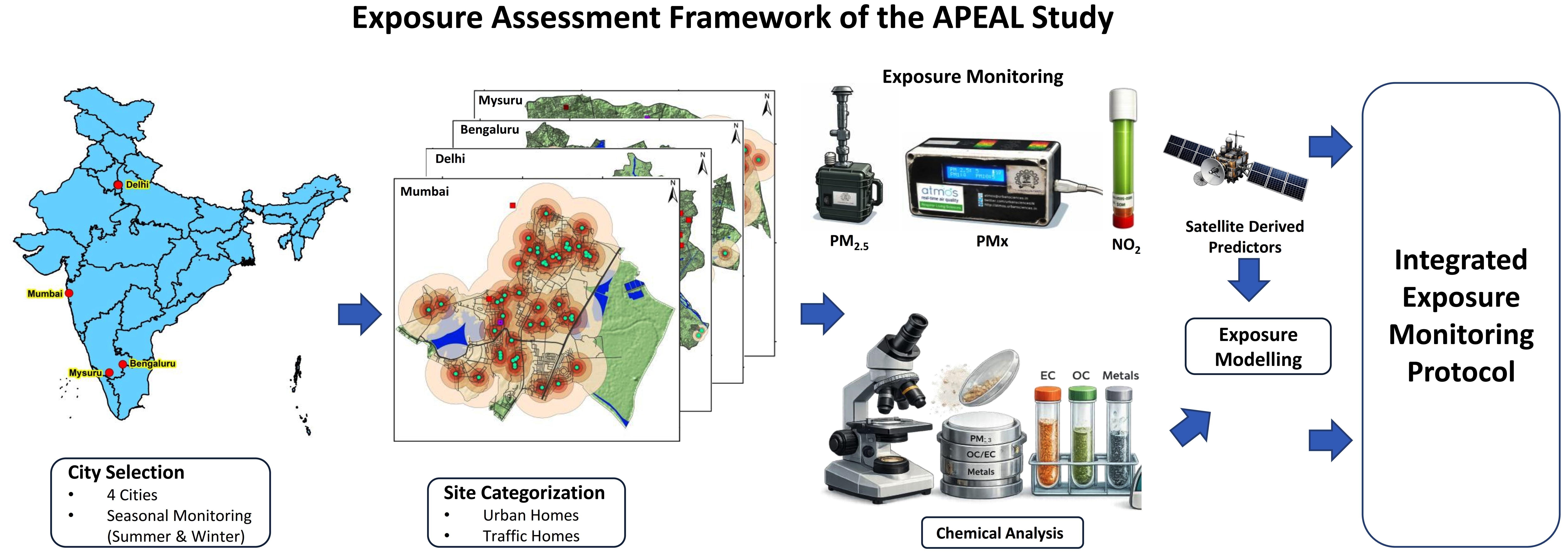
Rapid urbanization intensified spatial variability in air pollution across India, while monitoring networks are limited in capturing local exposure conditions. This study develops and evaluates an exposure assessment framework, with pilot findings from the Air Pollution Exposure on Adolescents’ Lungs (APEAL), a multi-centre prospective cohort study conducted in Delhi, Mumbai, Bengaluru, and Mysuru, which represent diverse air pollution levels. Residential measurements of fine particulate matter (PM2.5) and nitrogen dioxide (NO2) were conducted using standardized protocols. Results from pilot-phase showed that mean outdoor PM2.5 concentrations were highest in Delhi (90.4 ± 12.0 µg/m³), followed by Mumbai (57.2 ± 12.8 µg/m³), and Bengaluru (53.0 ± 9.0 µg/m³), with Mysuru having the lowest at 32.3 ± 9.3 µg/m³, indicating a north-south gradient attributed to anthropogenic activities. Optical properties of PM2.5, including absorption coefficients (Babs370 and Babs880), and calculated Absorption Angstrom Exponent (AAE), show significant variations and are primarily influenced by combustion sources. Further, this approach will include seasonal monitoring, chemical characterization, toxicity analysis, land-use regression (LUR) modelling, and time activity pattern to generate high-resolution exposure estimates. This methodology provides a robust, scalable framework for epidemiological studies and urban air pollution assessment in resource-limited settings, with relevance for urban planning and policy making.
Keywords:
air pollution exposure
; PM2.5
; optical properties
; NO2
; adolescents
; urban environment
; Indian cities
; APEAL study
1. Introduction
Long-term exposure to air pollutants, such as fine particulate matter (PM) with an aerodynamic diameter ≤ 2.5, and nitrogen dioxide (NO2), has been associated with a wide range of adverse health outcomes [1,2,3]. Fine particles can penetrate deep into the lungs, triggering inflammation and contributing to respiratory illness, cardiovascular disease, and premature deaths [4,5,6,7]. In addition to its health impacts, PMs also influence atmospheric visibility and alter the Earth’s radiative balance, contributing to uncertainty in climate projections [8,9]. Higher levels of air pollution from PM further increase public health risks by reducing visibility (causing traffic accidents) and increasing the incidence of respiratory diseases, especially in densely populated urban regions [10,11].
Carbonaceous fractions of PM2.5, particularly black carbon (BC) and brown carbon (BrC), result from incomplete combustion processes and significantly contribute to urban air pollution due to their strong light-absorbing properties [12,13]. These species are commonly emitted from traffic, fossil fuel use, and biomass burning, leading to their co-occurrence with high PM2.5 levels in urban environments. Studies conducted in Indian cities consistently show high PM2.5 concentrations and significant contributions from BC, indicating shared emission sources and co-variability in ambient air [12,13,14,15,16,17]. In addition, spectral absorption characteristics, including enhanced ultraviolet absorption linked to BrC and higher absorption Ångström exponent (AAE), further indicate the influence of biomass burning and mixed combustion sources on PM2.5 composition [13]. The presence of carbonaceous components in urban environments suggests that residents, especially adolescents, are consistently exposed to particulate matter derived from combustion. Several studies have shown that exposure to PM2.5 is linked with adverse respiratory outcomes, including reduced lung function and impaired lung development [18,19,20,21,22,23,24].
Most large epidemiological studies on air pollution have been conducted in Western countries, where traffic-related pollution levels are relatively moderate compared with those in many South Asian cities. At present, many cities in India face severe air quality issues due to emissions from vehicles, industries, and household fuels, which especially affect children’s health. PM2.5 levels in major metropolitan areas often surpass the World Health Organization’s (WHO) annual guideline of 10 µg/m³, reaching five to ten times higher than the standard. According to the WHO report, 11 cities in India rank among the 12 most polluted cities in the world [25]. This exposure is associated with higher risks of chronic respiratory conditions, including chronic obstructive pulmonary disease (COPD), and cardiovascular disease (CVD), contributing to increased medical costs, preventable illness, and premature mortality [26,27]. Persistently high pollution levels and associated public health risks indicate the need for in-depth research to identify vulnerable groups and to inform targeted interventions.
Over the past few decades, large cohort studies have played a key role in understanding the health effects of air pollution. One influential example is the Swiss SAPALDIA cohort, launched in 1991, which followed 9,651 adults from eight regions of Switzerland to track long-term respiratory and cardiovascular health [28]. The study found that sustained exposure to PM10, NO2, and O3 (ozone) was linked to reduced lung function, increased risks of asthma, COPD, and increased cardiovascular morbidity [28,29,30,31,32]. The study also demonstrated that cleaner air quality leads to measurable improvements in lung function and reduced respiratory symptoms [33]. The European Study of Cohorts for Air Pollution Effects (ESCAPE) is another pioneering study, initiated in 2008 across more than twenty European countries. It uses detailed exposure assessments and advanced modelling to estimate pollution exposure at residential locations. The study revealed a significant correlation between long-term exposure to PM2.5, PM10 and NO2 with various health issues, including higher risks of cardiovascular diseases, respiratory conditions, lung cancer, adverse birth outcomes (low birth weight and preterm delivery), and increased mortality rates [34,35,36,37,38,39,40]. During the early 2000s, the Multi-Ethnic Study of Atherosclerosis and Air Pollution (MESA Air) investigated the relationship between long-term exposure to air pollution and the development of CVD. The study examined over 6,000 participants from six major metropolitan areas of the United States, using advanced methods (monitoring and modelling) to assess individual exposure to PM2.5, NO2, and other pollutants [41,42]. Major finding of the MESA Air study showed a significant association between higher PM2.5 and increased coronary artery calcification, a key marker of atherosclerosis that raises the risk of heart attacks and cardiovascular events [43,44,45,46]. The Tamil Nadu Air Pollution and Health Effects (TAPHE) study in India investigated the health impacts of air pollution on approximately 1,200 to 1,500 pregnant women and their newborns [47]. It combined air quality measurements, health surveys, and clinical assessments to examine outcomes such as birth weight, gestational age, and respiratory health, among participants. Results indicated a significant relationship between parental exposure to air pollution and adverse birth outcomes, including low birth weight and preterm delivery, as well as a higher risk of respiratory infections in newborns [47,48,49].
In urban environments, children are most vulnerable to the adverse effects of air pollution. Several factors make children more susceptible to air pollution compared to adults. These include: a) developing lungs that are more sensitive to harmful substances, b) a larger lung surface area and the ability to inhale 50% more air, c) insufficient detoxification and cytoprotective capacity, and d) immature immune defences. After birth, the lungs continue to develop and mature quickly during adolescence (10-16 years), and an individual reaches peak lung function by 18-20 years of age. After that, lung function gradually decreases with age, starting from around 22-25 years old [50,51]. Furthermore, it can lead to significant deficits in lung function, as measured by forced expiratory volume (FEV), during the transition from childhood to young adulthood (18-22 years old) [52,53,54]. This reduction in lung function in early childhood leads to a three-times higher risk of COPD and CVD later in life. The CVD and COPD are the second leading causes of death in India, although the exact magnitude of the problem is currently unknown [55].
Many Indian cities are among the most polluted in the world, with air pollution levels 2–5 times higher than those in Western countries due to rapid urbanization, industrial growth, and increasing vehicular emissions, adversely affecting the lung health of urban children in India [48]. However, only a very few air pollution exposure cohort studies are being conducted in low- and middle-income countries, especially in India [47,56,57,58]. The pollution significantly affects respiratory and cardiovascular health, especially in vulnerable groups like children and elders, are a major public health concern. Poor lung function among adolescents constitutes a significant risk factor for early CVD, and the investigation of COPD prevalence in the Indian population remains an unexplored area of study. Therefore, it is an urgent need for an early predictive biochemical marker to identify individuals with poor lung function growth but remain asymptomatic. Identifying the high-risk children population would help in implementing remedial behaviors that could mitigate lung health throughout childhood, and this could also be the most effective public health strategy to reduce disease burden later in adult life.
A comprehensive cohort study is essential to generate robust scientific evidence on the long-term health effects of air pollution, informing effective policy interventions to improve air quality and public health. To address this gap, the APEAL (Longitudinal Effects of Air Pollution Exposure on Adolescent Lungs) study has been established as a prospective multi-city cohort study in India, enrolling approximately 5000 children aged 11–14 years from Delhi, Mumbai, Bengaluru, and Mysuru [59,60,61]. The study is designed to evaluate the impact of long-term exposure to PM2.5 (including its chemical characteristics, optical properties, and toxicity) and NO2 on pulmonary function, identify factors affecting lung growth, and develop models to estimate annual exposure levels.
Given the limited evidence base for exposure assessment, the manuscript presents the exposure assessment framework and pilot findings with the objectives of (i) quantifying spatial variability of PM2.5 and NO2 across diverse urban environments, (ii) characterizing the optical properties of PM2.5 to identify emission sources, and (iii) developing a comprehensive exposure assessment protocol combining monitoring, modelling, and time-activity data. In India, there are very few studies that investigate the prediction of air pollution exposure and its impacts on adolescents' lung health; therefore, the APEAL study is highly relevant and topical, with the potential to be a pioneering effort in this area of research.
2. Materials and Methods
2.1. Study Area Selection
India is a geographically and socioeconomically diverse country, with different cultures, food habits, lifestyles, and living environments. For the APEAL cohort study, four cities were selected based on reported air pollution levels: very high (Delhi), high (Mumbai and Bengaluru), and moderate (Mysuru) (Figure 1).
Delhi (latitude 28o 40’ to 28o 88’ N to longitude 76o 84’ to 77o 35’ E), the national capital of India, ranks among the most polluted megacities globally, with mean annual concentrations of PM2.5 frequently beyond 100 µg/m³. The city covers approximately 1,488 km² and has a population exceeding 20 million within the larger National Capital Region (NCR). Delhi has a semi-arid and subtropical climate with prevailing winds predominantly from the west and northwest directions, and an average annual wind speed ranging from 0.9 to 2 m/s [62]. The annual average temperature is approximately 32 °C, with a maximum of 45 °C during the summer. Winter conditions are characterised by low temperatures, inversions, and stagnant meteorology, which facilitate the accumulation of pollutants [63]. The primary sources of emissions include vehicular pollution, power plants, industrial operations, construction dust, household fuel combustion, and seasonal biomass burning in adjacent states.
Mumbai city lies between latitude 18° 89’ to 19° 27’ N and longitude 72o 77’ to 72o 98’ E, is the financial hub of India, situated along the Arabian Sea. The city experiences a tropical coastal climate, characterised by high humidity and moderate temperature variations. Monsoon season in the city starts from June to September, with a total annual precipitation of approximately 2147 mm in the suburban region [64]. Mean annual temperature of the city is 27 oC. Despite coastal ventilation that promotes dispersion, Mumbai faces significant challenges to its air quality due to vehicular emissions, industrial activities in suburban areas, port operations, and resuspended road dust.
Bengaluru, located on the Deccan Plateau at an elevation of approximately 900 meters, experiences a moderate climate with clear wet and dry seasons. The city lies a longitude range of 77o 35’ E to 77o 73’ E and a latitude range of 12o 83’ N to 13o15’ N, covering an area of around 741 km². The climate of the city is classified as a tropical savanna (dry winter: Aw), characterized by distinct wet and dry seasons [65]. Rainfall is influenced by both the southwest and northeast monsoons, with the heaviest rainfall in August, September, and October [65]. Although Bengaluru was known previously as a low-pollution city, rapid urbanization, traffic congestion, and construction activity have led to rising levels of PM2.5 and NO2 in recent years.
Mysuru (12o 23’ to 12o 37’ N and 76o 58’ to 76o 72’ E), located approximately 145 km southwest of Bengaluru, is a medium-sized city with lower levels of industrilization and traffic density. The city has a mean elevation of 770 m and experiences a dry tropical to sub-tropical climate, with an average annual rainfall of 798 mm and temperatures ranging from 12 to 35°C [66]. For this study, Mysuru was considered a low-exposure setting due to its relatively lower industrial activity, moderate traffic, and meteorological conditions that support pollutant dispersion. In general, annual PM2.5 concentrations in Mysuru remain below 40 µg/m³.
The APEAL study areas are defined as a subset of cities with a population exceeding 200,000, encompassing both formal and informal settlements. This selection was made based on the delineation of ward and sub-ward boundaries, with the aim of providing a comprehensive reflection of the city's entire demographic composition (Figure 1).
2.2. Selection of Study Participants
Study participants were recruited through schools, health camps, and door-to-door outreach with support from community leaders, if they met the following criteria: (1) their ages ranges from 11-14 years; (2) they had no previously diagnosed respiratory diseases such as asthma, tuberculosis, chest wall deformities, severe cardiac illness (precluding performance of spirometry), or other serious diseases, and (3) they had recently moved or had been living in their current residences for less than one year. Detailed recruitment protocols for participants through schools and door-to-door visits are discussed elsewhere [59].
Each study centre aimed to enrol approximately 1200 children per city (a total of 4800), and around 60 subjects (each city) were strategically selected for daily indoor and outdoor PM2.5 monitoring as well as biweekly indoor and outdoor NO2 measurements conducted in their homes. The outdoor measurements will be taken in their balconies or fortified garden areas, and repeated at the same site in both the summer and winter seasons. The PM2.5 and NO2 levels will also be monitored at the selected schools of all four study cities during both seasons.
2.3. Selection of Monitoring Homes
The APEAL study employs the ESCAPE/SAPALDIA site-selection approach with modifications [67,68]. This methodology adopted in these studies enables standardization of methods and facilitates the comparison of exposure levels across European cities. In the APEAL study, a list of recruited participants from all centers will be collected along with geo-coordinates. The geocodes will be utilized to determine the normalized difference built-up index (NDBI) value for each specific site. The type of homes will then be identified using the previously explained method [36,67]. Homes will be selected based on the criterion that participants have lived there for more than one year. Additionally, preference will be given to homes that have balconies. Consent and availability will then be obtained from participants prior to measuring pollutant concentrations.
The sampling homes will be classified as traffic-exposed (~45 sites) and urban background (15 sites) based on their proximity to the road. Traffic-exposed homes will be identified using the criteria: (i) distance from motorway and trunk road is 500m, the major road is 300 m, and the secondary road is 200 m. (ii) road density around the home location, calculated within buffer zones of 1000 m for motorway and trunk roads is greater than or equal to 0.001 m/m2; for major roads under a buffer of 500 m is greater than or equal to 0.01 m/m2, and for the secondary road under a buffer of 200 m greater than or equal to 0.03 m/m2. (iii) traffic congestion value is greater than or equal to 2 (Figure 2). Traffic-exposed home sites will be overrepresented, as these sites are expected to be the most informative for developing stochastic exposure models. Urban background sites use the following criteria: (i) the distance between the sites is greater than 500 m from the motorway and trunk road, 300 m from the major road, and 200 m from the secondary road. (ii) the sites with NDBI value > 0.01 (Figure 2). One fixed site per city, located within the parent institute, will also be selected as a regional background site (away from major emission sources, including residential areas and traffic), for both PM2.5 and NO2 measurements.
2.4. Microenvironment Sampling
Children spend a significant portion of their day in the school environment, making it essential to conduct exposure sampling in this micro-environment. This is particularly important because children are more susceptible to the adverse effects of air pollution due to their developing respiratory systems, higher breathing rates, and longer periods spent engaged in outdoor activities. Therefore, monitoring air quality in schools is crucial for accurately evaluating exposure and potential health risks.
In the APEAL study, PM2.5 and NO2 levels will be monitored both indoors and outdoors at selected schools in each city, following a consistent residential exposure monitoring protocol. One classroom of study participants will be selected from each school for indoor sampling, and for outdoor measurements, a suitable location will be identified to capture exposure data effectively.
2.5. Sampling Schedule
The APEAL study implements a structured monitoring methodology to measure pollutant levels in both summer and winter, capturing seasonal changes in air quality across the study areas. This approach effectively captures temporal variations within the study areas, enhancing the accuracy of exposure assessments and aiding the development of land-use regression (LUR) models that predict pollutant exposure for each participant [34]. In the study, indoor and outdoor PM2.5 measurements will be conducted for ∼24 hours during both the summer and winter seasons. Simultaneously, NO2 passive samplers will also be deployed for a 14-day integrated measurement across all sites. Before the extensive seasonal measurements, a pilot study was conducted to establish comprehensive protocols and methodologies to accurately determine each participant's exposure levels throughout the study. The detailed analysis and discussion of the pilot-phase NO2 monitoring results are presented elsewhere [61].
2.6. Monitoring Instruments and Methodology
2.6.1. Particulate Matter (PM2.5) and PMx
PM2.5 concentration at outdoor and indoor locations will be collected on polytetrafluoroethylene (PTFE) and quartz fiber filter substrates for ∼24 hr at each site using low-volume air sampler (AirMetric, Oregon, USA), operating at 6 L/min. PM2.5 mass will be obtained by pre- and post-weighing of PTFE filter substrates. Filters will be pre-conditioned at 25°C and 50% relative humidity (RH) for 24 hours prior to weighing with a Micro Balance (Sartorius Cubis MSU6.6S; sensitivity 1μg). All loaded quartz filters will undergo thermal/optical carbon analysis to measure organic carbon (OC) and elemental carbon (EC). This analysis will follow the IMPROVE-A protocol (Interagency Monitoring of PROtected Visual Environments) on a multi-wavelength analyzer (DRI Model 2015) [7,69].
A total of ~150 daily outdoor and indoor filters (including 15% field blanks and duplicates) will be collected from each study center per season, resulting in a total of ~1400 daily samples from all locations. PM mass, black carbon (BC), and trace elements will be collected on Teflon filters and analysed using gravimetric, optical transmission, and inductively coupled plasma-atomic emission spectroscopy (ICP-AES) methods, respectively. The first two methods are non-destructive; thus, multiple analyses can be performed after splitting the collected filters for various analyses, including oxidative potential (OP) assessment. Similarly, the quartz filter samples will be analyzed for inorganic ions and elemental and organic carbon using ion chromatography (IC), and EC-OC thermal optical transmission (TOT) analysis methods, respectively. The following equation is used to calculate the concentration of PM2.5 for all sites:
where Mf and Mi represents the final and intial mass (mg) of the conditioned filter, 103 represents unit conversion factor for milligrams (mg) to micrograms (μg), Qavg represents average flow rate over the entire duration of the sampling period (L/min), t represents duration of sampling period (min), and 10-3 represents unit conversion factor for liters (L) into cubic meters (m3).
As the measurement of PM2.5 spans 20-22 days, comparing daily averages within cities is not feasible. Therefore, a background temporal correction will be applied using the following expression [38]:
where Ccri represents corrected PM2.5 concentration at ith site, CAvgRBG represents average PM2.5 concentration at regional background for all sampling periods, and CRBG represents concentration of PM2.5 at regional background site measured on the same day as Ci.
Real-time monitoring of indoor PMx (PM1, PM2.5, and PM10) levels will also be simultaneously conducted across all locations using ATMOS, a cost-effective sensor developed by Urban Sciences. The ATMOS sensor also captures air temperature and humidity, with precise geographic coordinates and time. The device transmits the recorded data to the cloud server in real-time through a built-in GPRS/GSM module and the HTTP protocol. The comprehensive details regarding the instruments, calibration processes, measurements and the results of the pilot phase conducted for the APEAL study are thoroughly discussed elsewhere [70].
2.6.2. PM2.5 Optical Properties
PM can both scatter and absorb shortwave radiation due to its composition and structural characteristics. Scattering leads to atmospheric cooling, whereas absorption causes a positive radiation anomaly that contributes to warming [59]. Further, atmospheric warming enhances stability, degrades air quality, and poses both short- and long-term health risks [13,71,72,73].
After gravimetric analysis of PM2.5 samples, optical attenuation (ATN) at 880 nm and 370 nm will be measured using an OT-21 transmissometer (Magee Scientific, USA) instrument, to determine the absorption coefficients (Babs) at each wavelength, enabling the estimation of the light-absorbing properties of PM2.5 [13,74,75]. To calculate the Babs for the specified wavelength in the study, the methodology adopted by Manwani et al. [13] and Bharadwaj et al. [76] are utilized.
where ATN represents measured attenuation, A represents the effective filter area (m2), V represents volume of air sampled (m3), Babs represents absorption at λ, Cλ represents scattering correction factor, Rλ represents shadowing correction factor, and AAE represents Absorption Angstrom Exponent.
The attenuation was analysed at wavelengths 370 and 880 nm, and bATN was calculated using equation 3. To calculate the Babs, λ, R will be determined using equation 6, and for C, an iterative procedure will be employed using equations 7 and 8, starting by assuming C = 1 at the start. The Cref is set at 1.4845 at 428nm [13]. Finally, AAE will be calculated using equation 8. The absorption coefficients will be used to examine the properties of carbonaceous aerosols, including black carbon (BC) and ultraviolet particulate matter (UVPM), with higher optical absorption indicating the presence of brown carbon (BrC), typically associated with biomass burning [13,77].
2.6.3. Nitrogen Dioxide (NO2)
Indoor and outdoor NO2 concentrations will be monitored using passive diffusion samplers (PDS), developed by the Passam ag, M€annedorf, Switzerland. (www.passam.ch) [61]. Passive sampling is suitable for large-scale deployment due to its low cost, no power requirements, operate unattended, and ability to produce accurate results. Additionally, PDS provide a significant advantage for conducting long-term simultaneous measurements of pollutant concentrations across multiple sites within an extensive geographical area [78,79,80,81,82]. The PDS collects NO2 by molecular diffusion through an inert tube to an absorbent triethanolamine (TEA). In use, the samplers are mounted vertically, and the lower cap is removed at the start of sampling, allowing NO2 to diffuse through the tube and react with TEA, which captures it. At the end of the sampling period, the tube is sealed again, and the absorbed NO2 is determined spectrophotometrically by the well-established Griess-Saltzmann method [82]. The deployment framework for indoor and outdoor passive samplers is discussed in detail elsewhere [61]. The following equation will be used to determine the NO2 concentration:
where K represents standardization factor (micrograms of NO2 per mL of absorbing solution/ absorbance), Vr represents volume of air sampled under standard conditions (L), and v represents volume of sample (mL). To calculate Vr, following equation is used:
where V represents volume of air sampled at ambient conditions (L), P represents average ambient atmospheric pressure(kPa), T represents average ambient atmospheric temperature (K), 101.3 is the pressure of standard atmosphere (kPa), and 290.15 is the temperature of standard atmosphere (K).
During the pilot phase, indoor and outdoor sample tubes (n=50) from 7-9 homes/city were collected and tested in both the PASSAM ag and the IITB laboratories to assess method precision and results. The agreement between methods and their comparison is discussed in detail in the supplementary section. Further, during seasonal measurements, a total of 240 home outdoor and indoor biweekly NO2 samples (including 10% blanks and duplicates) will be collected from each study centre, resulting in ~500 outdoor and indoor home NO2 sample tubes across all four study centres. Additionally, ~100 biweekly NO2 samples will be collected at a central background location from all four study centres. Of the collected NO2 samples, 15% will be sent to the Passam ag laboratory, while the remaining samples will be analysed in our lab using the Greiss-Saltzmann method by photospectrometry.
In this study, seasonal measurements will be conducted to assess the variability observed throughout the year. Further, the annual average concentrations were calculated using the formula:
where, represents the annual average concentration at ith site and jth city, and represents the concentration measured at ith site in the summer and winter seasons, respectively, andrepresents the CPCB concentration on that day in the summer and winter seasons, respectively. Details regarding the NO2 measurement process and results of the APEAL pilot study are discussed in Vijay et al. [61].
2.7. Oxidative Potential (OP)
Oxidative stress, characterized by an imbalance between the amount of reactive oxygen species (ROS) production and the body’s antioxidant defences [83,84,85], and the resulting inflammatory response represent a key biological mechanism involved in PM-induced health effects [85,86,87,88]. Oxidative potential (OP) reflects the capacity of PM to generate ROS in biological systems and represents an initial step in understanding downstream oxidative stress and inflammatory responses [85].
Various studies have identified OP as a key indicator for air quality regulations [85]. Therefore, the APEAL study also incorporates PM2.5-derived OP as an additional metric of particle toxicity alongside mass concentration. By assessing the extent and distribution of PM-derived OP, the study establishes OP as an independent metric of external exposure that complements conventional pollutant measurements. Detailed laboratory procedure for OP analysis is provided in Supplementary Section S1.
2.8. Chemical Analysis (Ions and Metals)
PM2.5 is a complex mixture of various chemical components, has been closely linked with adverse respiratory and cardiovascular health outcomes, contributes significantly to the global burden of diseases [89,90,91]. In the APEAL study, PTFE filters will be used to assess water-soluble inorganic ions (WSII) and trace metals, following established protocols [92,93,94]. WSIIs and trace metals constitute major components of PM2.5 mass and influence its acidity and overall toxicity. Analyzed WSIIs include cations such as Na+, K+, Mg2+, NH4+, Ca2+ and anions Cl-, Br-, NO3-, NO2-, PO43- and SO42-. Further, metals are classified into two categories: water-soluble metals (designated as Group A) and acid-digestible metals (designated as Group B). The metal ions included in this analysis are Ca²⁺, Al³⁺, Fe²⁺, Mn²⁺, Se⁴⁺, Sr²⁺, Pb²⁺, Ni²⁺, Cu²⁺, Co²⁺, As³⁺, Zn²⁺, Cd²⁺, Cr³⁺, V⁵⁺, and Mo3+. This analysis aims to determine the overall concentrations of metals (Groups A and B) present in PM2.5 particles. Detailed analytical procedures are provided in the Supplementary Section S2.
2.9. Heavy Metals in Hair and Nails
To assess internal exposure and dosage of PM in children, as well as to compare them with external exposure, biological samples such as hair and nails will be collected from a subset of participants. The standard operating procedure (SOP) for sample collection is detailed elsewhere [59]. This subgroup will constitute about 10% of the study population, with approximately 120 subjects per city. Hair samples will be collected near the root using stainless steel scissors, with each sample weighing approximately 0.5 grams. Nail samples will be taken from all ten fingers by trimming them with clean nail clippers. Samples will be stored in labelled plastic bag with the proper ID at room temperature until analysis. Samples (hair and nails) were subjected to a microwave-assisted acid digestion procedure similar to the one used for PM2.5 samples [95]. Subsequently, the levels of toxic heavy metals in these bio-samples will be measured using ICP-AES and ICP-MS methods as discussed in the previous section. The procedures are discussed in detail in elsehwhere [96].
Further, heavy metal levels measured in the various school and home environments will be compared with concentrations found in hair and nail samples to assess how exposure to polluted microenvironments is reflected in these biomarkers. Spearman’s correlation coefficients will then be used to asses association between environmental exposure and biomarker concentrations.
2.10. Questionnaire
During sampling, each participant will complete a structured questionnaire with four sections: (i) demographic information, (2) household characteristics, (iii) kitchen and cooking practices, and (iv) 24-hour activity pattern. Household charecteristics include the age of the house, number of floors, doors, and windows, as well as the presence and use of air conditioning (AC). Information on kitchen usage covers daily cooking time, cooking frequency, and the type of fuel or energy source for cooking. The 24-hour recall documents cooking-related exposure and other indoor activities, such as burning incense, diya or candles, mosquito coils, and routine cleaning activities like sweeping and mopping. Ventilation practices will also be recorded, including the number of windows and the duration of their opening during cooking. The questionnaire further captures outdoor factors that may influence indoor air quality, including trash burning, smoke from neighbours, vehicular traffic along the street, and local construction and industrial activity. During school monitoring, the questionnaire collects general information about the school’s infrastructure, classroom environment, cleanliness, outdoor conditions, and the behaviours of both students and staff.
The APEAL questionnaire will collect detailed time-location information from each participant. Each participant reports the amount of time they spend at home, at school, travelling between home and school, and in after-school activities. Additionally, the questionnaire records other locations outside their homes and schools where they spend time. These data will be used to adjust individual exposure estimates based on time spent indoors (reflected by the infiltrated concentrations) and time spent outdoors (indicated by the ambient concentrations measured at the participants’ homes and schools). Most information is primarily collected from parents, although a small number of questions can be answered directly by the children. Data will be collected using a digital survey platform (Go Survey application) for efficient data management. Full details of the household and school characteristics questionnaire will be captured during monitoring and are provided in the Supplementary Annexure I and II.
2.11. Quality Assurance and Quality Control (QA/QC)
Mini-volume (MiniVol) samplers will be routinely calibrated to ensure accurate flow rates for precise sampling. All filters will be transported to and from the central laboratory in separate sealed Petri dishes, maintaining a cool temperature throughout. To ensure accuracy, blank and duplicate samplers will also be deployed for time-integrated measurements, at a rate of 10% from fixed and home sites for both PM2.5 and NO2. Furthermore, our instrument will also be co-located with at least one reference monitoring station within the study area for quality control. The NO2 sampling principle is based on Fick’s law of diffusion. Duplicate tubes will deploy to assess the precision of the method, and a subset of the total tubes will be forwarded to Passam ag. (Switzerland) for inter-laboratory comparison to evaluate quality and accuracy. The analysis of NO2 will be conducted using the Modified Saltzmann method (EN16339:2013). All measurements will be conducted by the same core team, using identical instruments, standardised sampling protocols, and criteria for the selection of sampling sites. Filters will be discarded under the following circumstances: if the instrument has operated < 20 hours, if it has functioned for only a few hours, if it has been dropped, or if it has experienced any malfunctions.
2.12. Development of Land Use Regression (LUR) Models
Due to limited air quality monitoring coverage, mathematical modelling approaches are widely used to estimate pollution exposure. These models provide a practical alternative to the high cost and logistical demands of continuous monitoring [97,98]. The model can also represent both the spatial distribution of air pollutant concentrations and individual exposure levels. Therefore, modelling approaches are especially useful in areas where monitoring stations are sparse or absent [98,99]. GIS is widely utilized in air pollution modeling because it captures fine-scale spatial variation of pollutant distribution [34,35]. Over recent decades, land-use regression (LUR) has become one of the most widely applied techniques for estimating annual averages of pollutants such as NO₂, NOx, SO₂, PM₁₀, PM2.5, and VOCs [36,67,99,100,101,102]. The LUR model combines measurements from a limited set of monitoring sites (the dependent variable) with GIS-based predictors (independent variables) to construct statistical models of spatial pollution patterns.
The present study will develop LUR models that incorporate measured air pollution data, GIS parameters, land-use characteristics, and meteorological parameters to estimate both indoor and outdoor exposures of each participant at their home and school locations. Selection of predictor variables for the LUR models will be based on previous studies and on univariate regression analyses of each potential predictor.
2.12.1. Predictor/Independent Variables
Various datasets derived from GIS and satellite-based indices will be prepared as potential predictors for the development of the LUR model. Data corresponding to each participant will be extracted within buffer zones(100-5000 m) around each participant's location.
Previously, various studies uses predictor variables such as population density [103,104], road proximity [105,106], road density [107,108,109], land use/land cover [110,111,112], land surface temperature [112,113], normalized difference vegetation index [114,115], altitude [116,117], and meteorological parameters [118,119] to develop LUR model. This study will examine various factors, including population density (PD), traffic-related variables such as proximity to roads (RB) and road density (RD), land surface temperature (LST), topography (T), the normalized difference vegetation index (NDVI), land use/land cover (LU/LC), meteorological variables, and continuously monitored levels of PM2.5 and NO2 to develop LUR models. A detailed list of these predictors, along with their data sources, is provided in Table 1.
2.12.2. Land-Use Regression (LUR) Model
LUR models estimate pollutant levels at specific locations based on the environmental characteristics of the surrounding area. This method depends on geospatial data to build predictive models widely used in environmental and epidemiological research [105,120]. The LUR models are typically developed by linking measured pollutant concentrations from monitoring sites with GIS-derived predictor variables through regression analysis. In the present study, multiple linear regression (MLR) with a supervised stepwise selection procedure will be used to construct the LUR models for predicting pollutant concentrations. The stepwise regression was selected to prioritise interpretability and consistency with established LUR methodologies, whereas the supervised procedure allows controlled inclusion of predictors based on statistical significance and physical probability, supporting a transparent evaluation of the spatial determinants of air pollution [34,36,40].
In the APEAL study, daily and annual models will be developed to estimate outdoor and indoor exposure to PM2.5, NO2, black carbon (BC), and brown carbon (BrC). Toxicity metrics, such as OPDTTv and OPAAV, will also be incorporated to assess PM2.5 toxicity for all participants. A time-weighted exposure model will be developed to more accurately capture individual exposure. This will account for the time spent in various microenvironments, such as indoors, outdoors, at school, and during travel, each characterized by different pollutant concentrations. Predictor or independent variables for these models include PD, RB, RD, LU/LC, LST, NDVI, altitude (T), meteorological data, and information collected through questionnaires.
Standard diagnostic procedures for ordinary least squares regression will be applied to examine heteroscedasticity and influential observations. An illustration of the general LUR model function, depicting the predicted levels of annual outdoor pollutants based on various predictor variables, will be utilized in the APEAL study and is presented below:
where, represents the predicted concentration of pollutants (PM2.5, NO2, Babs340-880, OP) at location i, and city j, X represents predictor variables such as population density (PD), road proximity (RP), road density (RD), land use/land cover (LU/LC), normalized difference vegetation index (NDVI), land surface temperature (LST) and altitude (T) at the location i, and represent the coefficients of the predictor variables that indicate its influence on the pollution level.
In the daily model, the CPCB pollutant concentrations and meteorological variables are added to the above-mentioned annual predicted variables. The equation for the determination of the indoor pollution exposure model is as follows:
where, is the predicted value of the indoor pollution level at micro-environment m in city j, represents outdoor pollutant concentration, Z represents indoor predictors such as smoking (S), ventilation characteristics (VC), indoor characteristics (IC), represents cooking frequency (CF), building characteristics (BC), and window opening frequency/duration (WOF).
Time-weighted average exposure (TWAE) levels for each pollutant in each city will be calculated from indoor and outdoor concentrations, weighted by the time participants spent in each microenvironment.
where, TWAE represent time-weighted average exposure (ng/m3) at location i, city j, and pollutant k represents the concentration of pollutants indoors, represents outdoor concentration, represents time spent indoors, represents time spent outdoors, and represents total time in a day (in hours).
All models will run separately, and performance will be measured using leave-one-out cross-validation (LOOCV) method in terms of mean difference (±SD) between measured and estimated concentrations, adjusted R2, and RMSE value. All area-specific models will be built to estimate daily and annual-average pollutant concentrations to predict annual air pollution exposures for all recruited participants.
2.12.3. Exposure Prediction
Various studies indicated that personal exposure is influenced by both indoor and outdoor sources, as well as individual activities and time spent in different microenvironments [41,121]. In the APEAL study, a hybrid exposure model will be developed that integrates indoor and outdoor PM2.5 and NO2 measurements to estimate air pollution exposure among children enrolled in the APEAL cohort.
Predictor variables for the LUR models will be defined based on prior literature and a univariate regression analysis of each potential predictor. Using the collected PM2.5 datasets, models for daily and annual outdoor, indoor, source, and absorption (370 and 880) exposure models will be developed. Measured NO2 data will also be utilized for the development of biweekly and yearly models of outdoor NO2 exposure and indoor NO2 exposure models. Finally, a personal time-weighted exposure model will be developed by integrating the time-activity profiles of each study participant based on geocode and other relevant predictors, along with both outdoor and indoor measurements. The time-weighted exposure model provides a more accurate assessment of the overall exposure of participants by integrating exposure levels across microenvironments (home, ambient, and school). The details of the methodology adopted for the development of LUR and the prediction of pollutants is depicted in Figure 3.
2.13. Statistical Analysis and Software
Inter-city comparison will be conducted by one-way ANOVA followed by post hoc tests, while the difference between the sites will be evaluated using an independent t-test. Pearson correlation will be calculated to assess the correlation between the predictors and the response variables. For regression, the ordinary least squares (OLS) regression method will be used in Python to perform LUR models. The Python 3.11.9 environment will be used for model development. All statistical analyses were performed using Excel, SPSS, and Python. Spatial processing, including delineation and estimation of predictor variables, will be carried out using ArcGIS (version 10.8) and QGIS (version 3.30.1), while Origin (version 2022) will be used for graphical representation of the results.
3. Results
During the pilot phase of the APEAL study, residential indoor and outdoor PM2.5 air pollution measurements were conducted for ∼24 hours at 7-9 homes across 7 consecutive days in each city during April-May 2022. Simultaneously, NO2 samplers were also deployed for 7 days at all homes, one city at a time. The results of the Pilot study presented here both spatial and temporal variability, along with a preliminary characterization of PM optical properties, supported by standardized sampling protocols and quality-controlled measurements.
3.1. Spatial Variability of PM2.5 Concentrations
Pilot measurement revealed substantial spatial variability in outdoor PM₂.₅ concentrations across study cities. Mean PM2.5 (±SD) mass concentrations were highest in Delhi (90.4 ± 12.0 µg/m³), followed by Mumbai (57.2 ± 12.8 µg/m³) and Bengaluru (53.0 ± 9.0 µg/m³), while Mysuru exhibited the lowest levels (32.3 ± 9.3 µg/m³). A one-way ANOVA indicated a significant difference in PM2.5 concentrations among cities (F (3,30) = 39.24, p < 0.001). Tukey’s HSD test indicated that Delhi had significantly higher concentrations than all other cities (p < 0.001), while Mysuru had significantly lower levels than Mumbai and Bengaluru (p < 0.01). No significant difference was found between Mumbai and Bengaluru (p > 0.05). Distribution of sampling sites and their respective PM2.5 concentration is shown in Figure 4. Differences in PM2.5 concentration across cities were statistically significant (P < 0.05). These findings indicate a pronounced north-south gradient, likely reflecting differences in anthropogenic emission intensity, meteorological conditions, and urban characteristics among the cities.
3.1.1. Daily Variation of PM2.5
Daily PM2.5 concentrations measured over the 7-day pilot period showed clear inter-city and intra-city variability across residential, background, and central monitoring station (CMS) sites (Figure S1). Mean residential outdoor PM2.5 concentrations in all cities were significantly higher (p< 0.05) than the fixed-site regulatory monitoring station level. Figure S1 shows systematic differences between measurement methods, with APEAL exposure assessment shows greater variability and consistently higher concentrations than CMS. This observation suggests that measurement methodology substantially influences reported air pollution levels. The findings indicate that the Central Pollution Control Board (CPCB) monitoring stations may underestimate APEAL residential outdoor PM2.5 exposure. This discrepancy may be attributed to the limited spatial coverage of monitoring networks, their concentration in specific urban locations, and their inability to capture fine-scale spatial variability. These limitations highlight the need for more spatially resolved and representative monitoring approaches to accurately assess population exposure.
In Mysuru, residential PM2.5 concentrations were consistently lower in all homes among all four cities, with median values ranging from ~16.5 to 44.6 μg/m3, remaining below the national daily standard (60 μg/m3) (Figure S1). Only one house (H6) exceeded the daily standard on a single day, whereas other homes showed no exceedances during the monitoring period. Background and CMS measurements also showed low concentrations with minimal variability, indicating relatively uniform ambient conditions across the city. In Bengaluru, residential PM2.5 concentrations were moderate but spatially heterogeneous, with median levels ranging from ~26.5 to 65.3 μg/m³. Four out of seven homes exceeded the daily standard at least once, with one home (H5) exceeding it on five days, and two others (H6 and H7) on three and four days, respectively. Background concentrations were lower than residential measurements, and CMS measurements exhibited lower variability, smoothing localized peaks observed in residential monitoring. PM2.5 concentrations in Mumbai were consistently higher than in Mysuru and Bengaluru, with median values ranging from ~46.4 to 71.6 µg/m3 across homes. Several residential sites exceeded the daily standard, with five out of nine homes recorded exceedances during the monitoring period. Two homes (H4 and H8) exceeded the daily standard on 5 out of 7 days, while others exceeded for 1 to 3 days. Background concentrations were lower than most residential measurements, whereas CMS concentrations showed lower variability, despite the high pollution burden of the city. Delhi exhibited the highest PM2.5 concentrations among all cities, with median levels ranging from ~86.4 to 112.2 µg/m3, substantially exceeding the national daily standard. All homes exceeded this standard for 6 to 7 days during the monitoring period, with locations H3, H4, H6, and H7 surpassing it every day. Background and CMS concentrations were also consistently elevated, though less variable than residential levels, indicating more stable conditions at the monitoring sites.
3.1.2. Comparison Between 7-Day Mean vs 1-Day (PM2.5)
During the pilot phase, PM2.5 concentrations were monitored simultaneously at multiple sites within each study area for a continuous 7-day period. Residential measurements showed greater variability and more frequent exceedances compared to background and CMS observations (Figure S1). Although CMS concentrations represented overall city-level pollution, they underestimated both the magnitude and frequency of exceedances observed at residential locations. Mean values, shown within each box, were often higher than the medians, particularly in Mumbai and Delhi. This pattern indicates right-skewed distributions, driven by occasional high-pollution events.
Figure 5 complements these findings by summarizing the absolute % deviation of individual daily PM2.5 measurements from their corresponding 7-day mean values. In most locations across cities, daily PM2.5 concentrations showed only slight variation from the 7-day average. Median deviations were also low, with only a few outliers exhibiting higher deviations (> 20%).
Statistical comparisons (Supplementary Tables S1–S4) indicated that only a limited number of daily measurements differed significantly from their corresponding 7-day means (Figure 5). These findings indicate that one-day PM2.5 measurements are largely representative of the 7-day average concentrations during the stable summer season. Further, these results support the use of short-term PM2.5 measurements for characterizing longer-duration exposure in pilot studies. However, it is important to recognize that occasional episodic events may introduce short-term variability that is not fully captured by single-day sampling.
3.1.3. Distribution of Babs370 and 880 at Outdoor Residential Sites
Residential outdoor absorption coefficients measured at 370 nm (Babs370) and 880 nm (Babs880) exhibited pronounced inter-city and intra-city variability across the four study cities (Figure 6a-d). Median Babs880 values showed a clear north-south gradient, with the highest levels in Delhi, followed by Mumbai and Bengaluru, and the lowest in Mysuru. Across residential sites, Babs880 ranged from approximately 100–300 Mm⁻¹ in Delhi, 120–280 Mm⁻¹ in Mumbai, 90–220 Mm⁻¹ in Bengaluru, and 80–180 Mm⁻¹ in Mysuru, highlighting substantial contrasts in exposure to combustion-derived light-absorbing aerosols (Table S4-S8).
This spatial pattern closely reflects the inter-city differences in PM2.5 mass concentrations observed during pilot phase study and is consistent with previous Indian measurements of black carbon (BC) and absorption coefficients. Urban studies in Delhi have reported summer Babs880 (or BC-equivalent absorption) values ranging from 150 to >400 Mm⁻¹, driven primarily by vehicular emissions, diesel combustion, and resuspended road dust mixed with combustion particles [122,123]. In contrast, measurements from southern Indian cities such as Bengaluru and Chennai typically report lower absorption coefficients (∼80-200 Mm⁻¹), reflecting lower combustion intensity and differences in source profiles [124,125]. These observations reinforce the role of local emission intensity in shaping residential exposure gradients.
Across all cities, Babs370 values were consistently higher than Babs880 at nearly all residential locations, often exceeding them by 30–70 % (Figure 6a-d). This pattern indicates a significant contribution from UV-absorbing organic aerosols, commonly referred to as brown carbon (BrC) (Table S5-S8). In Delhi and Mumbai, several residential sites exhibited Babs370 values exceeding 250–400 Mm⁻¹, suggesting enhanced contributions from biomass burning, residential fuel use, and secondary organic aerosol formation in addition to fossil fuel combustion. Similar wavelength-dependent absorption behavior has been reported in Indian megacities, where BrC contributions to near-UV absorption can account for 20-40% of total aerosol light absorption, particularly during summer and transition seasons [126,127,128]. These findings are consistent with global urban observations. Measurements from Asian megacities such as Beijing and Shanghai report Babs880 values of 150–350 Mm⁻¹, with substantial enhancement at short-wavelength absorption attributed to BrC from mixed combustion sources [127]. In contrast, European and North American cities typically exhibit lower absorption coefficients (∼30–120 Mm⁻¹), reflecting stricter emission controls and lower BC burdens [128]. The observed Babs magnitude in this study suggests that Indian urban residential exposures are among the highest globally.
In addition to inter-city differences, significant variability was observed with many residential areas showing wide interquartile ranges during the 7-day sampling period (Table S4-S8). This micro-scale variability is influenced by proximity to roads, traffic density, local combustion activities, and urban morphology. Background (BG) sites exhibited lower, less variable absorption coefficients than residential sites, indicating the influence of localized emission sources on household-level exposure. Similar spatial heterogeneity in BC and absorption coefficients has been reported in dense urban areas, where residential exposure can differ significantly from central monitoring locations [129,130].
Combined analysis of Babs370 and Babs880 shows significant differences in residential outdoor exposure to light-absorbing carbonaceous aerosols within and across cities. The consistency of these findings with previous Indian and global studies validates the pilot design and supports the inclusion of multi-wavelength optical absorption measurements in the full-scale APEAL exposure assessment. Importantly, the observed spatial heterogeneity reinforces the need for neighborhood-scale monitoring to accurately evaluate exposure to combustion-related aerosols and their potential health impacts in longitudinal cohort studies.
3.1.4. Comparison Between 7-Day Mean vs 1-Day mean (Babs370 and Babs880)
Figure 6 (a-d) presents the absolute % deviation of daily Babs370 and Babs880 concentrations from their respective seven-day mean values across Bengaluru, Delhi, Mumbai, and Mysuru. Across all cities, the distributions exhibit relatively low median deviations with interquartile ranges generally confined within ~10–25%, indicating limited day-to-day variability in aerosol light absorption at both wavelengths. Although higher deviations were occasionally observed, particularly at sites in Mumbai and Delhi, these represent isolated events rather than sustained departures from weekly mean conditions. The constrained spread of deviations suggests that daily Babs₃₇₀ and Babs₈₈₀ measurements generally approximate weekly average absorption characteristics during the study period. Single t-tests were applied to evaluate deviations of individual daily observations from the corresponding weekly mean concentrations (Supplementary Tables S5–S8). Only a limited number of days across cities and monitoring sites showed statistically significant deviations (Figure 6 a-d). The limited number of significant deviations indicates that large variations in daily Babs370 and Babs880 from weekly averages were uncommon during the study period. These findings indicate that single-day measurements provide a reasonably reliable representation of short-term absorption characteristics under stable conditions in this study.
3.1.5. Absorption Angstrom Exponent (AAE)
Previous studies indicate that the AAE for urban aerosols and motor vehicle emissions is typically close to 1 (0.7 to 1.2), reflecting weak spectral dependence [131,132,133,134,135,136,137]. AAE values close to or below 1 are generally associated with carbonaceous aerosols, such as BC from fuel combustion, whereas higher values indicate contributions from BrC, often linked to biomass burning, and secondary organic aerosols [138,139].
In this study, AAE was calculated using Eq. (8), and results indicated that the average measured AAE370-880nm (±SD) values for Delhi, Mumbai, Bengaluru, and Mysuru are 0.83 ± 0.10, 1.01 ± 0.22, 0.83 ± 0.18, and 1 ± 0.17, respectively (Figure 7). AAE values across Delhi indicate a predominantly mixed aerosol regime, reflecting contributions from both fossil fuel combustion (traffic emissions) and biomass burning, with values above ~1.4 are typically associated with enhanced brown carbon influence (Table S9-S12). In Mumbai, AAE values (0.90–1.19) indicate a dominant influence of fossil-fuel and traffic emissions, with most homes showing values close to unity. Homes such as H6-H9 show higher AAE, indicating occasional biomass burning, while generally low variability indicates stable emission sources, except at H8, where higher variability suggests episodic influences. In Bengaluru, mean AAE values range from 0.73 to 0.95, mostly below 1.0, indicating that fossil fuel and traffic emissions are the primary contributors, with minimal input from biomass burning. Low variability across all sites suggests stable emission sources, whereas the higher variability at site B4 indicates episodic fluctuations. The mean AAE values in Mysuru range from 0.90 to 1.12, primarily reflecting the influence of fossil fuel and traffic-related aerosols, with some impact from biomass burning at sites like H2 and H5. Most sites exhibited low variability, indicating consistent emission sources, except H4, which shows higher variability, suggesting an episodic event. Mysuru has less influence from biomass burning than larger urban areas, largely driven by local combustion sources.
Figure 7 illustrates the temporal variations observed across different monitoring sites and sampling days. In all cities, the percentage deviation of AAE remained below 20% on most days, indicating relatively stable day-to-day variability. A site-specific analysis for AAE was also conducted using a t-test on daily observations to compare them with the corresponding 7-day mean (Table S9-S12). Unlike Babs370 and Babs880, none of the daily AAE values from any city showed significant differences from their weekly averages. These results indicate that AAE is temporally stable, suggesting that a single-day measurement is a reliable representation of the seven-day average. This reinforces the reliability of short-term observations for characterizing AAE in this study and further supports the practice of conducting measurements on a single day during seasonal assessments.
In addition to mass concentration and AAE, the pilot study investigated chemical analyses of carbonaceous components (OC and EC), water-soluble inorganic ions (WSII), toxicity (Oxidative potential), and elements in PM2.5 samples. Mass reconstruction or mass closure is also performed to validate chemical speciation and to understand the PM2.5 composition of the pilot study samples. These findings are discussed in detail in a separate manuscript currently in submission.
3.2. NO2 Measurements and Inter-Laboratory Comparison
NO₂ measurements were conducted as part of the APEAL study pilot phase using passive diffusion samplers deployed for 7-day integrated sampling, representing weekly average levels. Collected sampler tubes were analysed at both PASSAM ag and IIT Bombay (IITB) laboratories, and inter-laboratory agreement was evaluated using the Bland–Altman (BA) method. Results from the BA analysis indicated a mean difference of 3.3 µg/m³ between PASSAM ag and IITB–Shimadzu measurements [140], showing a small positive bias in PASSAM ag results (Figure S2). The LoA ranged from −19.5 to 26.2 µg/m³, within which the majority of paired observations were distributed, indicating acceptable agreement between the two analytical methods across the observed concentration range (Figure S2).
During the pilot study, the highest outdoor NO2 levels were observed in Mumbai (67.4 ± 24.1 µg/m³) and Bengaluru (66.8 ± 20.9 µg/m³), followed by Delhi (61.2 ± 8.4 µg/m³), while Mysuru recorded the lowest concentrations (32.4 ± 11.6 µg/m³) (Figure 8). These differences reflect variations in traffic density, urban activity, and emission sources across cities. Additional analyses of indoor and outdoor NO2 and volatile organic compounds (VOCs), as well as correlations (indoor/outdoor) for BTEX (benzene, toluene, ethylbenzene, and xylene), except in Mumbai, were conducted and presented in detail elsewhere [61].
3.3. Correlation
The relationships between PM₂.₅ concentrations, absorption coefficients, NO₂, and VOCs across three cities (Delhi, Bengaluru and Mysuru) are presented in Figure 9(a, c, d). BTEX sampling was not conducted in Mumbai due to limited sampler availability; therefore, correlations for Mumbai (Figure 9b) are shown without BTEX, while analyses for the other cities include these compounds.
The correlation matrix for Delhi (Figure 9a) indicates that PM₂.₅ is moderately positively associated with NO₂ and black carbon (Babs₃₇₀ and Babs₈₈₀), suggesting dominant contributions from traffic and combustion sources. A very strong correlation between Babs₃₇₀ and Babs₈₈₀ (r = 0.96) confirms a common origin from black carbon emissions. AAE shows weak and negative associations with most pollutants, suggesting a dominance of fossil-fuel combustion with limited variability in source types. Strong inter-correlations among VOCs (r = 0.72–0.92) further indicate shared emission sources, whereas PM₂.₅ shows negative correlations with VOCs (r = 0.72-0.92), particularly p-xylene, indicating either differing emission sources or their involvement in secondary aerosol formation. Correlation pattern for Mumbai (Figure 9b) shows that PM₂.₅ is strongly positively correlated with Babs₃₇₀: (r ≈ 0.90), and Babs₈₈₀ (r ≈ 0.88), indicating a dominant contribution from combustion-related sources, especially vehicular emissions and fossil fuel burning . A moderate positive correlation is observed with NO₂ (r ≈ 0.45–0.55), supporting the influence of vehicular emissions. The correlation between Babs₃₇₀ and Babs₈₈₀ is very high (r > 0.95), confirming a common source of light-absorbing carbon, whereas AAE shows a weak correlation with PM₂.₅ (r ≈ 0.10–0.20), suggesting relatively uniform source characteristics dominated by fossil fuel combustion. Bengaluru (Figure 9c) also shows positive correlations with Babs₃₇₀ (r = 0.87) and Babs₈₈₀ (r = 0.86), and a moderate correlation with NO₂ (r = 0.69), highlighting the dominant influence of traffic and combustion-related emissions. In addition, VOCs (benzene, toluene, ethylbenzene, and xylenes) show moderate positive correlations with PM₂.₅ and strong inter-correlations among themselves (r = 0.65–0.92), suggesting shared emission sources such as vehicular exhaust and fuel evaporation. The negative correlations among AAE, PM2.5 and other pollutants indicate a dominance of fossil-fuel combustion, with a limited contribution from biomass burning. Whereas, correlation matrix for Mysuru (Figure 9d) indicates weak associations of PM₂.₅ with Babs₃₇₀, Babs₈₈₀ and NO₂, suggesting a relatively lower influence of direct combustion emissions compared to other cities. In contrast, PM₂.₅ shows moderate positive correlations with VOCs (r = 0.39–0.51), indicating a stronger contribution from VOCs-related sources or secondary formation processes. The strong inter-correlations among VOCs species (r = 0.69–0.90) suggest common emission sources, likely including vehicular emissions.
4. Discussion
Pilot-phase monitoring results indicate substantial spatial variability in PM₂.₅ and NO₂ exposure across four urban environments with distinct emission profiles, highlighting pronounced heterogeneity at both inter-city and microenvironmental scales. Mean PM2.5 concentrations ranged from 32.3 µg/m³ in Mysuru to 90.4 µg/m³ in Delhi, reflecting differences in traffic intensity, industrial activity, built-up density, and regional meteorological conditions. In Delhi, summer PM2.5 levels are attributed to traffic, industrial activities, dust, and other combustion sources, along with contributions from regional and long-range transport [141,142]. Vehicular emissions are a major source of PM2.5 in Mumbai city, with additional contributions from heavily trafficked road corridors and industrial activities [143,144]. In Bengaluru, local emissions, including those associated with black carbon, are reported to impact PM2.5 levels [145]. PM2.5 and NO2 concentrations in Mysuru are associated with proximity to major roads, local point sources, and areas with higher human activity and population density, whereas regions with less activity tend to have lower levels [146,147]. These findings indicate that exposure patterns vary between cities and underscore the need for location-specific modeling approaches rather than general assumptions about air pollution exposure.
Comparison between 1-day and 7-day PM2.5 averages during the summer pilot period showed minor deviations at most sites, suggesting that short-term sampling, when temporally adjusted using background data, can provide reliable spatial contrasts in exposure. This finding has practical implications for exposure mapping during large-scale seasonal monitoring campaigns, particularly in resource-limited settings. Furthermore, the analysis of optical properties (AAE) indicated that combustion-related sources were particularly dominant in highly polluted areas. Additionally, an inter-laboratory comparison of NO₂ measurements showed good agreement, supporting the reliability of passive sampling methods.
Residential monitoring showed greater variability and more frequent exceedances of national daily air quality standards than central monitoring stations. While regulatory sites capture broader urban trends, they tend to smooth local peaks influenced by road proximity, land-use configuration, and neighbourhood sources. Thus, relying solely on fixed monitoring stations may underestimate fine-scale differences in exposure. High-resolution predictors, such as road density, proximity to major roads, LST, NDVI, and population density, will be essential for improving the performance of LUR models across diverse urban environments.
Building characteristics, ventilation practices, and indoor combustion sources significantly influence exposure variability. These findings support the development of hybrid exposure models that integrate outdoor spatial predictions with microenvironment-specific adjustment factors derived from questionnaires and house characteristics. Incorporating chemical composition, optical properties, and oxidative potential expands exposure assessment beyond mass-based metrics, enabling improved source attribution and health-relevant characterization.
Relationship between ambient pollutants such as PM2.5 and NO2 with adverse cardiovascular health effects is well established [148,149]. Unlike many previous cohort studies, such as SAPALDIA (Switzerland) [28,150], ESCAPE (Europe) [34,35,36,37,38,39,40], MESA Air (USA) [41,42,43], and TAPHE (India) [47,48], which predominantly concentrate on adult populations or early-life exposure within high-income or single-city contexts. On the other hand, APEAL represents one of the first longitudinal study in India to specifically focus on the adolescent group, which is very important for studies related to lung development and respiratory functions.
Previously, epidemiological studies relied largely on outdoor monitoring and simple exposure models; APEAL adopts a more comprehensive exposure assessment framework. It integrates indoor and outdoor measurements of PM2.5 and NO₂, along with time-activity patterns, chemical composition, optical properties, and toxicity indicators, across four cities (Delhi, Mumbai, Bengaluru, and Mysuru) that represent diverse pollution levels, urban forms, and meteorological conditions. While studies such as ESCAPE and SPALDIA established a widely used framework for standarized exposure assessment in well-monitored urban settings, their focus on annual averages and outdoor concentrations may not fully capture exposure dynamics in low- and middle-income countries. These studies primarily relied on outdoor LUR models based on fixed-site monitoring and long-term background data, which are effective for capturing regional pollution gradients in cities with well-developed regulatory networks [28,34,68,103]. In contrast, the APEAL study is designed to address these limitations by incorporating seasonal variability, microenvironmental contributions, and geospatial predictors, including satellite-derived data and low-cost sensor measurements, to better represent uneven monitoring coverage common in many Indian cities. Further, APEAL will combine both indoor and outdoor residential measurements of PMx and NO2, along with individual time-activity patterns, and detailed chemical, optical, and toxicological characterisation of PM2.5. This integration gives a complete understanding of individual exposure in environments where households and microenvironments significantly contribute to overall pollution levels.
Traffic-related emissions are a major contributor to air pollution variability within urban areas, which may significantly impact cardiovascular morbidity and mortality [151,152,153,154]. Given the high vulnerability of adolescents to poor lung health, the findings from the APEAL study could support the implementation of public health measures that require routine lung function screening for children through high school. This would aid in early detection and identifying those at higher risk for COPD or CVD later in life. Furthermore, the study emphasizes the importance of moving beyond mass-based metrics by incorporating measures of PM toxicity into air quality assessment, which allows a more comprehensive evaluation of health risks associated with urban air pollution.
4.1. Methodological Innovations
This manuscript describes the exposure assessment approach developed for the APEAL study, addressing a major gap in air pollution epidemiology research in low- and middle-income countries, such as India.
A major strength of the study is its multi-city design, encompassing Delhi, Mumbai, Bengaluru, and Mysuru, representing significant variations in air pollution levels, emission sources, meteorology, urban structures, and socioeconomic conditions. This diversity improves the study's external validity and captures spatial patterns often ignored in single-city studies, and allows for assessing exposure-response relationships at higher pollution levels. The study also uses a strategic site selection method adopted from the ESCAPE and SPALDIA studies to categorize urban locations by their proximity to roads and developed regions, allowing for accurate air pollution measurements. The exposure assessment strategy has significant methodological advancements compared to previous cohort studies, which primarily relied on outdoor concentration.
The APEAL study integrates simultaneous outdoor and indoor measurements at both home and school microenvironments. Previously, large cohort studies relied primarily on outdoor concentrations derived from fixed-site regulatory stations. In contrast, this framework accounts for indoor environments where adolescents spend a substantial portion of their time. By measuring pollutant levels directly in homes and classrooms, the study captures exposure variability driven by household characteristics, ventilation practices, cooking behavior, and building design. This approach allows a more accurate estimation of total exposure in urban settings, where indoor sources can significantly influence pollutant concentrations. Seasonal monitoring design is another strength of this study, capturing pollutant concentrations in cities during both summer and winter. This approach effectively captures the temporal variability and meteorological influences in the cities. Further, the framework combines gravimmetric mass measurement with detailed chemical analyses of PM2.5, including chemical characterization, optical properties, and oxidative potential. In addition to determining mass concentration, the study evaluates carbonaceous fractions (OC/EC), water-soluble inorganic ions (WSII), trace metals, light absorption properties (at 370 nm and 880 nm), and multiple oxidative potential assays (DTT, AA, and LPO). Incorporating toxicity metrics with bio-sample (hair and nails) analysis provides biological significance to particle composition, strengthening the linkage between urban emission sources and potential health implications.
The study will also develop hybrid exposure models that integrate measured pollutant concentrations with LUR modelling, satellite-derived indicators, GIS-based spatial predictors, and meteorological variables. By integrating direct measurements with spatial predictors, the framework enables estimation of daily and annual pollutant concentrations at high spatial resolution, even in cities with limited regulatory monitoring coverage. Additionally, developing 24-hour time-weighted average exposure models that incorporate adolescents' individual activity patterns. Questionnaire-based time-activity data are used to adjust exposure estimates according to time spent indoors, outdoors, at school, and in transit. This microenvironment-based adjustment reduces exposure misclassification and improves representation of inhaled dose compared with models based solely on residential outdoor concentrations. The study compares 1-day PM2.5 measurements with 7-day means during the pilot phase, showing that short-term sampling with background correction can effectively represent weekly exposure. This finding supports the cost-effective monitoring strategies in resource-limited urban areas while maintaining acceptable accuracy. Inter-laboratory validation of NO2 measurements using the Bland-Altman method to assess the agreement between both analyses is also one of the major findings of the methodology framework. This step strengthens quality assurance and enhances confidence in cost-effective passive sampling methodologies deployed across multiple cities.
Strong attention to QA and QC, including the use of field blanks and duplicates during PM2.5 and NO2 monitoring, inter-laboratory comparisons, co-location of monitoring instruments, standardised protocols and centralised training for field staff, also strengthens the study. These innovations, along with a consistent framework for the APEAL study, support the adaptation of the methodology to other rapidly urbanising regions.
4.2. Limitations
While the APEAL study has several strengths, it comes with some limitations as well. First, while we are able to reasonably capture both indoor and outdoor exposures using 24-hrs measurements for each resident/school, longer measurement periods will capture the within-home variability better. Our pilot study results established that 24-hrs measurements (compared with weekly exposure) can significantly capture long-term exposure, but are less comprehensive than extended measurements. Second, although gravimetric PM2.5 samples will be collected in homes, quartz-specific sampling will not be undertaken in indoor environments due to practical and logistical constraints, including limitations related to instrumentation, space, and the need to minimize disruption to participating households. Third, a staggered monitoring design is also a limitation, as it may introduce temporal confounding, which we address by applying the background temporal correction adopted from the SPALDIA study [28]. While the study extends the usual outdoor exposure to total individual exposure utilizing time activity patterns and microenvironment measurements, its validation will require measurement through wearable personal devices. Fourth, the universal limitation of exposure studies is measurement error, and exposure misclassification can also lead to uncertainty into exposure estimates, particularly due to the temporal and spatial variability of pollutant concentrations and the challenge of accurately capturing all relevant microenvironments. Finally, long-term follow-up in urban populations poses challenges related to mobility and participant retention. However, standardised protocols, training, and regular follow-ups every six months are employed to keep participants engaged and enrolled.
Standardized protocols, a consistent methodology, and focused training for field staff will ensure reliable measurement of environmental exposures and health outcomes, limit measurement error and bias. Although the study requires specific instruments and technical skills, the protocol provides a clear framework that can be adapted for future air pollution studies in low- and middle-income countries.
5. Conclusion
Despite significant advances in understanding the health effects of air pollution, evidence from adolescents in low- and middle-income countries remains limited, as most large cohort studies (SAPALDIA, ESCAPE, MESA Air, TAPHE, etc) have been conducted in high-income settings with different emission sources, regulatory frameworks, and exposure patterns. The APEAL study addresses this gap by being the first multi-city, prospective cohort in India, designed to evaluate how sustained exposure to urban air pollution influences respiratory development in this vulnerable age group. This study presents a framework for assessing urban exposure in four Indian cities, integrating indoor and outdoor monitoring at residential and school locations, chemical characterization, and spatial modeling that reflects distinct pollution regimes. Pilot results reveal significant inter- and intra-city variability in pollutant concentrations. Outdoor PM₂.₅ concentrations were highest in Delhi (90.4 ± 12.0 µg/m³), followed by Mumbai (57.2 ± 12.8 µg/m³) and Bengaluru (53.0 ± 9.0 µg/m³), while Mysuru showed lower levels (32.3 ± 9.3 µg/m³). Residential measurements showed greater variability and more frequent exceedances of the national daily standard (60 µg/m³) than central monitoring stations, indicating that fixed-site regulatory networks may underestimate localized exposure. Comparison of daily and seven-day PM₂.₅ averages during the pilot study showed minimal deviation (mostly < 20%) at most sites, indicating that short-term measurements can approximate longer-term exposure under stable conditions. This supports the feasibility of one-day monitoring during a seasonal campaign in resource-constrained settings. Optical analysis further indicated the dominance of combustion-related sources, particularly in highly polluted cities.
Integrating microenvironment measurements, chemical and toxicity characterization, GIS-based predictors, and individual time-activity data, the proposed framework provides a scalable and transferable approach for exposure assessment. This framework can be adapted to other rapidly urbanizing cities in low- and middle-income countries facing similar challenges. The findings can guide health measures such as improving school ventilation, reducing exposure in high-traffic areas, and maintaining cleaner indoor environments.
Supplementary Materials
The following supporting information can be downloaded at the website of this paper posted on Preprints.org.
Author Contributions
Conceptualization, H.C.P.; P.A.M., G.D., A.M., T.A., G.A.W., R.T. and A.N.S.; methodology, A.K., R.S. and H.C.P., software, A.K., and R.S., validation, A.K., and R.S., formal analysis, A.K., data curation, A.K. and R.S., writing-original draft preparation, A.K., R.S., V.S., P.V. and H.C.P.; visualization, A.K. and R.S.; supervision, H.C.P.; P.A.M., G.D., A.M., T.A., G.A.W., R.T. and A.N.-S.; project administration, H.C.P.; P.A.M., G.D., A.M., T.A. and R.T.; funding acquisition, H.C.P.; P.A.M., G.D., G.A.W., A.N.S., and A.M.
Funding
This research was funded by the Team Science from DBT Wellcome Trust India Alliance grant (RD/0120- DBT0001-004).
Ethics statement
Ethical approval for the study has been taken from the Institute Ethics Committee of the Indian Institute of Technology, Bombay (Approval No.: IITB-IEC/2021/013; Dated: 29-04-2021), JSS Medical College, Mysuru (Approval No: JSSMC/IEC/180820/04NCT/2020–21 Dated 20-08-2020), St. Johnʹs Medical College Hospital, Bengaluru (Approval No: IEC/1/184/2021 Dated 01-03-2021), All India Institute of Medical Sciences, New Delhi (Approval No: IEC-359/ 08.05.2020, RP-59/2020, Dated: 01/09/2020). No animals were used in this research, and all biosafety procedures will be followed when handling and storing biological samples.
Acknowledgments
We sincerely appreciate the support and contributions from all the research staff at our collaborating institutions: Indian Institute of Technology (IIT), Bombay; St Johns Medical College, Bengaluru; JSS Academy of Higher Education and Research, Mysuru; and All India Institute of Medical Sciences (AIIMS), Delhi, India.
Conflicts of Interest
The authors declare that they have no known competing financial interests or personal relationships that could have appeared to influence the work reported in this paper.
Abbreviations
The following abbreviations are used in the manuscript:
| APEAL | Air Pollution Exposure on Adolescents’ Lungs |
| BA | Bland Altman |
| BC | Black Carbon |
| BrC | Brown Carbon |
| COPD | chronic obstructive pulmonary disease |
| CPCB | Central Pollution Control Board |
| CVD | Cardiovascular Disease |
| ESCAPE | European Study of Cohorts for Air Pollution Effects |
| FEV | Forced Expiratory Volume |
| GIS | Geographic Information System |
| IC | Ion Chromatography |
| ICP-AES | Inductively Coupled Plasma-Atomic Emission Spectroscopy |
| ICP-MS | Inductively Coupled Plasma-Mass Spectrometry |
| LST | Land Surface Temperature |
| LoA | Limit of Agreement |
| LU/LC | Land use/Land cover |
| LUR | Land-use Regression |
| MESA Air | Multi-Ethnic Study of Atherosclerosis and Air Pollution |
| NCR | National Capital Region |
| NDBI | Normalized Difference Built-up Index |
| NDVI | Normalized Difference Vegetation Index |
| NO2 | Nitrogen Dioxide (NO2) |
| O3 | Ozone |
| OP | Oxidative Potential |
| PDS | Passive Diffusion Samplers |
| PD | Population Density |
| PM | Particulate Matter |
| RD | Road Density |
| ROS | Reactive Oxygen Species |
| SAPALDIA | Swiss Study on Air Pollution and Respiratory Diseases in Adults |
| SDGs | Sustainable Development Goals |
| TAPHE | Tamil Nadu Air Pollution and Health Effects |
| UVPM | Ultraviolet Particulate Matter |
| VOCs | Volatile Organic Compounds |
| WHO | World health Organization |
| WSII | Water-soluble Inorganic Ions |
References
- Pope, C. A., III; Burnett, R. T.; Turner, M. C.; Cohen, A.; Krewski, D.; Jerrett, M.; Thun, M. J. Lung cancer and cardiovascular disease mortality associated with ambient air pollution and cigarette smoke: shape of the exposure–response relationships. Environmental health perspectives 2011, 119(11), 1616–1621. [Google Scholar] [CrossRef]
- Kaufman, J. D.; Adar, S. D.; Barr, R. G.; Budoff, M.; Burke, G. L.; Curl, C. L.; Watson, K. E. Association between air pollution and coronary artery calcification within six metropolitan areas in the USA (the Multi-Ethnic Study of Atherosclerosis and Air Pollution): a longitudinal cohort study. The Lancet 2016, 388(10045), 696–704. [Google Scholar] [CrossRef] [PubMed]
- Xu, C.; Zhao, J.; Liu, P. A geographically weighted regression approach to investigate the effects of traffic conditions and road characteristics on air pollutant emissions. Journal of Cleaner Production 2019, 239, 118084. [Google Scholar] [CrossRef]
- Pope, C. A., III; Ezzati, M.; Dockery, D. W. Fine-particulate air pollution and life expectancy in the United States. New England journal of medicine 2009, 360(4), 376–386. [Google Scholar] [CrossRef] [PubMed]
- Kumar, A.; Krishna, A. P. Winter seasons assessment of atmospheric aerosol over Coalfield region of India using geoinformatics. Urban climate 2017, 20, 94–119. [Google Scholar] [CrossRef]
- de Prado Bert, P.; Mercader, E. M. H.; Pujol, J.; Sunyer, J.; Mortamais, M. The effects of air pollution on the brain: a review of studies interfacing environmental epidemiology and neuroimaging. Current Environmental Health Reports 2018, 5, 351–364. [Google Scholar] [CrossRef]
- Raparthi, N.; Phuleria, H. C. Real-world vehicular emissions in the Indian megacity: Carbonaceous, metal and morphological characterization, and the emission factors. Urban Climate 2021, 39, 100955. [Google Scholar] [CrossRef]
- Carslaw, D. C.; Williams, M. L.; Tate, J. E.; Beevers, S. D. The importance of high vehicle power for passenger car emissions. Atmospheric environment 2013, 68, 8–16. [Google Scholar] [CrossRef]
- IPCC. Summary for policymakers. In Climate change 2013: The physical science basis. Contribution of Working Group I to the Fifth Assessment Report of the Intergovernmental Panel on Climate Change; Stocker, T. F., Qin, D., Plattner, G.-K., Tignor, M., Allen, S. K., Boschung, J., Nauels, A., Xia, Y., Bex, V., Midgley, P. M., Eds.; Cambridge University Press, 2013; pp. 3–29. [Google Scholar]
- Tao, J.; Gao, J.; Zhang, L.; Zhang, R.; Che, H.; Zhang, Z.; Hsu, S. C. PM 2.5 pollution in a megacity of southwest China: source apportionment and implication. Atmospheric Chemistry and Physics 2014, 14(16), 8679–8699. [Google Scholar] [CrossRef]
- Feng, Y.; Ning, M.; Lei, Y.; Sun, Y.; Liu, W.; Wang, J. Defending blue sky in China: Effectiveness of the “Air Pollution Prevention and Control Action Plan” on air quality improvements from 2013 to 2017. Journal of environmental management 2019, 252, 109603. [Google Scholar] [CrossRef]
- Ambade, B.; Sankar, T. K.; Sahu, L. K.; Dumka, U. C. Understanding sources and composition of black carbon and PM2. 5 in urban environments in East India. Urban Science 2022, 6(3), 60. [Google Scholar] [CrossRef]
- Manwani, P.; Venkataraman, C.; Phuleria, H. C. Impact of open-field biomass burning on regional air quality in Northern India. Journal of Environmental Sciences 2025, 158, 126–136. [Google Scholar] [CrossRef] [PubMed]
- Tiwari, S.; Hopke, P. K.; Pipal, A. S.; Srivastava, A. K.; Bisht, D. S.; Tiwari, S.; Attri, S. D. Intra-urban variability of particulate matter (PM2.5 and PM10) and its relationship with optical properties of aerosols over Delhi, India. Atmospheric Research 2015, 166, 223–232. [Google Scholar] [CrossRef]
- Joshi, H.; Naja, M.; Singh, K. P.; Kumar, R.; Bhardwaj, P.; Babu, S. S.; Chandola, H. C. Investigations of aerosol black carbon from a semi-urban site in the Indo-Gangetic Plain region. Atmospheric Environment 2016, 125, 346–359. [Google Scholar] [CrossRef]
- Bhardwaj, A.; Haswani, D.; Yadav, K.; Raman, R. S. PM2. 5 carbonaceous components and mineral dust at a COALESCE network site-Bhopal, India: Estimating site-specific optical characteristics. Science of the Total Environment 2023, 880, 163277. [Google Scholar] [CrossRef]
- Kumar, B. S. K.; Rao, D. B.; Gayatri, B.; Prabakaran, N.; Chari, N. V. H. K.; Laxmi, C. N.; Gupta, G. V. M. Linking Chemical Composition, WSOC and Optical Behaviour of PM2. 5 Pollution Sources in Coastal Atmosphere at Kochi, India. Environmental Pollution 2026, 127965. [Google Scholar] [CrossRef]
- Balakrishnan, K.; Steenland, K.; Clasen, T.; Chang, H.; Johnson, M.; Pillarisetti, A.; Peel, J. L. Exposure–response relationships for personal exposure to fine particulate matter (PM2· 5), carbon monoxide, and black carbon and birthweight: an observational analysis of the multicountry Household Air Pollution Intervention Network (HAPIN) trial. The Lancet Planetary Health 2023, 7(5), e387–e396. [Google Scholar] [CrossRef]
- Paisi, N.; Kushta, J.; Pozzer, A.; Violaris, A.; Lelieveld, J. Health effects of carbonaceous PM2. 5 compounds from residential fuel combustion and road transport in Europe. Scientific Reports 2024, 14(1), 1530. [Google Scholar] [CrossRef]
- Guo, T.; Chen, T.; Chen, L.; Liu, J.; Song, X.; Zhang, Y.; Ma, J. Association between long term exposure to PM2. 5 and its components on severe obesity in Chinese children and adolescents: a national study in China. Children 2024, 11(12), 1536. [Google Scholar] [CrossRef]
- Zhou, X.; Zhang, X.; Bai, G.; Dong, G.; Li, X.; Chen, R.; Fu, J. Long-term exposure to fine particulate matter (PM2. 5) components and precocious puberty among school-aged children: Cross-sectional study. JMIR public health and surveillance 2025, 11(1), e62861. [Google Scholar] [CrossRef]
- Norzaee, S.; Kermani, M.; Hopke, P. K.; Ghorbanian, A.; Yunesian, M.; Kalantary, R. R.; Shahsavani, A. Association between exposure to PM2. 5 and Black Carbon and risk of Childhood Leukemia in Tehran, A Case-Control Study with Critical Exposure Time Windows. Environmental Research 2025, 123168. [Google Scholar] [CrossRef] [PubMed]
- Madani, N. A.; Carpenter, D. O.; Khwaja, H. A. Health Risk Assessment of PM2. 5, NO2, and BC Exposure on Adults and Children in Karachi, Pakistan. Urban Science 2026, 10(2), 97. [Google Scholar] [CrossRef]
- Liu, K.; Luo, H.; E, B.; Kuang, H.; Zhang, C.; Guo, X. Long-term exposure to PM2. 5 and NO2 and risk of myopia in Chinese school-aged children: a cross-sectional study. BMC ophthalmology 2026, 26(1), 54. [Google Scholar] [CrossRef] [PubMed]
- WHO. Ambient (outdoor) air pollution database, 2018 update; World Health Organization, 2018. [Google Scholar]
- Collaborators, G. B. D.; Ärnlöv, J. Global burden of 87 risk factors in 204 countries and territories, 1990–2019: a systematic analysis for the Global Burden of Disease Study 2019. The Lancet 2020, 396(10258), 1223–1249. [Google Scholar] [CrossRef]
- Pandey, A.; Brauer, M.; Cropper, M. L.; Balakrishnan, K.; Mathur, P.; Dey, S.; Dandona, L. Health and economic impact of air pollution in the states of India: the Global Burden of Disease Study 2019. The Lancet Planetary Health 2021, 5(1), 25–38. [Google Scholar] [CrossRef]
- Zemp, E.; Elsasser, S.; Schindler, C.; Kunzli, N.; Perruchoud, A. P.; Domenighetti, G.; SAPALDIA team. Long-term ambient air pollution and respiratory symptoms in adults (SAPALDIA study). American journal of respiratory and critical care medicine 1999, 159(4), 1257–1266. [Google Scholar] [CrossRef]
- Kuenzli, N. I. N. O.; Stutz, E. Z.; Perruchoud, A. P.; Braendli, O. T. T. O.; Tschopp, J. M.; Bolognini, G. I. A. N. F. R. A. N. C. O.; SPALDIA Team. Peak flow variability in the SAPALDIA study and its validity in screening for asthma-related conditions. American journal of respiratory and critical care medicine 1999, 160, 427–434. [Google Scholar] [CrossRef]
- Ackermann-Liebrich, U.; Kuna-Dibbert, B.; Probst-Hensch, N. M.; Schindler, C.; Dietrich, D. F.; Stutz, E. Z.; Sapaldia Team. Follow-up of the Swiss Cohort Study on Air Pollution and Lung Diseases in Adults (SAPALDIA 2) 1991–2003: methods and characterization of participants. Sozial-und Präventivmedizin/Social and Preventive Medicine 2005, 50, 245–263. [Google Scholar] [CrossRef]
- Downs, S. H.; Schindler, C.; Liu, L. J. S.; Keidel, D.; Bayer-Oglesby, L.; Brutsche, M. H.; SAPALDIA Team. Reduced exposure to PM10 and attenuated age-related decline in lung function. New England Journal of Medicine 2007, 357(23), 2338–2347. [Google Scholar] [CrossRef]
- Schindler, Christian; Keidel, Dirk; Gerbase, Margaret W.; Zemp, Elisabeth; Bettschart, Robert; Brändli, Otto; Brutsche, Martin H.; et al. Improvements in PM10 exposure and reduced rates of respiratory symptoms in a cohort of Swiss adults (SAPALDIA). American journal of respiratory and critical care medicine 2009, 179(no. 7), 579–587. [Google Scholar] [CrossRef]
- Schindler, C.; Kunzli, N.; Bongard, J. P.; Leuenberger, P.; Karrer, W.; Rapp, R. & Swiss Study on Air Pollution and Lung Diseases In Adults Investigators. Short-term variation in air pollution and in average lung function among never-smokers: the Swiss Study on Air Pollution and Lung Diseases in Adults (SAPALDIA). American journal of respiratory and critical care medicine 2001, 163(2), 356–361. [Google Scholar]
- Eeftens, M.; Beelen, R.; De Hoogh, K.; Bellander, T.; Cesaroni, G.; Cirach, M.; Hoek, G. Development of land use regression models for PM2.5, PM2.5 absorbance, PM10 and PM coarse in 20 European study areas; results of the ESCAPE project. Environmental science & technology 2012a, 46(20), 11195–11205. [Google Scholar]
- Eeftens, M.; Tsai, M. Y.; Ampe, C.; Anwander, B.; Beelen, R.; Bellander, T.; Hoek, G. Spatial variation of PM2.5, PM10, PM2. 5 absorbance and PMcoarse concentrations between and within 20 European study areas and the relationship with NO2–results of the ESCAPE project. Atmospheric environment 2012b, 62, 303–317. [Google Scholar] [CrossRef]
- Wang, M; Beelen, R; Basagana, X; Becker, T; Cesaroni, G; de Hoogh, K. Evaluation of land use regression models for NO2 and particulate matter in 20 European study areas: the ESCAPE project. Environ Sci Technol. 2013a, 47(9), 4357–64. [Google Scholar] [CrossRef] [PubMed]
- De Hoogh, K.; Wang, M.; Adam, M.; Badaloni, C.; Beelen, R.; Birk, M.; Hoek, G. Development of land use regression models for particle composition in twenty study areas in Europe. Environmental science & technology 2013, 47(11), 5778–5786. [Google Scholar]
- Eeftens, M.; Phuleria, H. C.; Meier, R.; Aguilera, I.; Corradi, E.; Davey, M.; Tsai, M. Y. Spatial and temporal variability of ultrafine particles, NO2, PM2. 5, PM2. 5 absorbance, PM10 and PMcoarse in Swiss study areas. Atmospheric environment 2015, 111, 60–70. [Google Scholar] [CrossRef]
- De Hoogh, K.; Chen, J.; Gulliver, J.; Hoffmann, B.; Hertel, O.; Ketzel, M.; Hoek, G. Spatial PM2.5, NO2, O3 and BC models for Western Europe–evaluation of spatiotemporal stability. Environment international 2018, 120, 81–92. [Google Scholar] [CrossRef]
- Gulliver, J.; Morley, D.; Dunster, C.; McCrea, A.; van Nunen, E.; Tsai, M. Y.; Kelly, F. J. Land use regression models for the oxidative potential of fine particles (PM2.5) in five European areas. Environmental research 2018, 160, 247–255. [Google Scholar] [CrossRef]
- Kaufman, J. D.; Adar, S. D.; Allen, R. W.; Barr, R. G.; Budoff, M. J.; Burke, G. L.; Tracy, R. P. Prospective study of particulate air pollution exposures, subclinical atherosclerosis, and clinical cardiovascular disease: the Multi-Ethnic Study of Atherosclerosis and Air Pollution (MESA Air). American journal of epidemiology 2012, 176(9), 825–837. [Google Scholar] [CrossRef]
- Krishnan, R. M.; Adar, S. D.; Szpiro, A. A.; Jorgensen, N. W.; Van Hee, V. C.; Barr, R. G.; Kaufman, J. D. Vascular responses to long-and short-term exposure to fine particulate matter: MESA Air (Multi-Ethnic Study of Atherosclerosis and Air Pollution). Journal of the American College of Cardiology 2012, 60(21), 2158–2166. [Google Scholar] [CrossRef]
- Hajat, A.; Diez-Roux, A. V.; Adar, S. D.; Auchincloss, A. H.; Lovasi, G. S.; O’Neill, M. S.; Kaufman, J. D. Air pollution and individual and neighborhood socioeconomic status: evidence from the Multi-Ethnic Study of Atherosclerosis (MESA). Environmental health perspectives 2013, 121(11-12), 1325–1333. [Google Scholar] [CrossRef]
- Kaufman, J. D.; Adar, S. D.; Barr, R. G.; Budoff, M.; Burke, G. L.; Curl, C. L.; Watson, K. E. Association between air pollution and coronary artery calcification within six metropolitan areas in the USA (the Multi-Ethnic Study of Atherosclerosis and Air Pollution): a longitudinal cohort study. The Lancet 2016, 388(10045), 696–704. [Google Scholar] [CrossRef]
- Sack, C.; Vedal, S.; Sheppard, L.; Raghu, G.; Barr, R. G.; Podolanczuk, A.; Kaufman, J. D. Air pollution and subclinical interstitial lung disease: the Multi-Ethnic Study of Atherosclerosis (MESA) air–lung study. European Respiratory Journal 2017, 50(6). [Google Scholar] [CrossRef]
- Kirwa, K.; Szpiro, A. A.; Sheppard, L.; Sampson, P. D.; Wang, M.; Keller, J. P.; Kaufman, J. D. Fine-Scale air pollution models for epidemiologic research: insights from approaches developed in the Multi-Ethnic Study of Atherosclerosis and Air Pollution (MESA Air). Current environmental health reports 2021, 8(2), 113–126. [Google Scholar] [CrossRef]
- Balakrishnan, K.; Sambandam, S.; Ramaswamy, P.; Ghosh, S.; Venkatesan, V.; Thangavel, G.; Team, S. C. Establishing integrated rural–urban cohorts to assess air pollution-related health effects in pregnant women, children and adults in Southern India: an overview of objectives, design and methods in the Tamil Nadu Air Pollution and Health Effects (TAPHE) study. BMJ open 2015, 5(6), e008090. [Google Scholar] [PubMed]
- Balakrishnan, K.; Ghosh, S.; Thangavel, G.; Sambandam, S.; Mukhopadhyay, K.; Puttaswamy, N.; Thanasekaraan, V. Exposures to fine particulate matter (PM2.5) and birthweight in a rural-urban, mother-child cohort in Tamil Nadu, India. Environmental research 2018, 161, 524–531. [Google Scholar] [CrossRef] [PubMed]
- Puttaswamy, N.; Natarajan, S.; Saidam, S. R.; Mukhopadhyay, K.; Sadasivam, S.; Sambandam, S.; Balakrishnan, K. Evaluation of health risks associated with exposure to volatile organic compounds from household fuel combustion in southern India. Environmental Advances 2021, 4, 100043. [Google Scholar] [CrossRef]
- Soremekun, S.; Heaney, L. G.; Skinner, D.; Bulathsinhala, L.; Carter, V.; Chaudhry, I.; Price, D. B. Asthma exacerbations are associated with a decline in lung function: a longitudinal population-based study. Thorax 2023, 78(7), 643–652. [Google Scholar] [CrossRef]
- Melén, E.; Faner, R.; Allinson, J. P.; Bui, D.; Bush, A.; Custovic, A.; Kermani, N. Z. Lung-function trajectories: relevance and implementation in clinical practice. The Lancet 2024, 403(10435), 1494–1503. [Google Scholar] [CrossRef]
- Oftedal, B.; Brunekreef, B.; Nystad, W.; Madsen, C.; Walker, S. E.; Nafstad, P. Residential outdoor air pollution and lung function in schoolchildren. Epidemiology 2008, 19(1), 129–137. [Google Scholar] [CrossRef]
- Gauderman, W. J.; Vora, H.; McConnell, R.; Berhane, K.; Gilliland, F.; Thomas, D.; Peters, J. Effect of exposure to traffic on lung development from 10 to 18 years of age: a cohort study. The Lancet 2007, 369(9561), 571–577. [Google Scholar] [CrossRef] [PubMed]
- Gouveia, N.; Junger, W. L.; Romieu, I.; Cifuentes, L. A.; de Leon, A. P.; Vera, J.; Tzintzun-Cervantes, G. Effects of air pollution on infant and children respiratory mortality in four large Latin-American cities. Environmental Pollution 2018, 232, 385–391. [Google Scholar] [CrossRef] [PubMed]
- Chakraborty, A.; Gupta, T. Chemical characterization and source apportionment of submicron (PM1) aerosol in Kanpur region, India. Aerosol and Air Quality Research 2010, 10(5), 433–445. [Google Scholar] [CrossRef]
- Prabhakaran, D.; Sieber, N. L.; Jaganathan, S.; Mandal, S.; Prabhakaran, P.; Walia, G. K.; Schwartz, J. D. Health effects of selected environmental Exposomes Across the Life course in Indian populations using longitudinal cohort studies: GEOHealth HEALS Study protocol. BMJ open 2024, 14(10), e087445. [Google Scholar] [CrossRef]
- Halder, P.; Verma, M.; Pal, S.; Mishra, A. K.; Deori, T. J.; Biswas, R.; Prabhakar, M. C. Association of anaemia with indoor air pollution among older Indian adult population: multilevel modelling analysis of nationally representative cross-sectional study. BMC geriatrics 2024, 24(1), 567. [Google Scholar] [CrossRef]
- Salve, H. R.; Dey, S.; Arora, Y.; Kapoor, S.; Ghosh, S.; Kumar, R.; Krishnan, A. Air Pollution Impact on Pregnancy and Early Childhood Development (APiPED) in India: Protocol for a Cohort Study. JMIR Research Protocols 2025, 14(1), e72683. [Google Scholar] [CrossRef]
- Agrawal, T.; Phuleria, H. C.; Mohan, A.; D’Souza, G.; Thimmulappa, R.; Jayaraj, B. S.; Mahesh, P. A. Rationale and methodology of a multicentric prospective cohort study on ‘Longitudinal Effects of Air Pollution Exposure on Adolescent Lungs (APEAL)’in urban India: APEAL protocol. BMJ open 2025, 15(8), e106329. [Google Scholar] [CrossRef]
- Mahesh, P. A.; Kaleem Ullah, M.; Greeshma, M. V.; Patil, S.; Samdarshi, P.; Veerabhadraiah, H.; Mohan, A. Prevalence of asymptomatic bronchial hyperresponsiveness in Indian adolescents: insights from the apeal study. Clinical & Experimental Allergy 2025, 55(9), 795–807. [Google Scholar] [CrossRef]
- Vijay, P.; Kumar, A.; Dubey, S.; Singh, R.; Sahota, V.; Borse, S.; Phuleria, H. C. Residential indoor and outdoor exposure to VOCs and NO2: insights from a multi-city pilot study in India. Environmental Geochemistry and Health 2026, 48(4), 181. [Google Scholar] [CrossRef]
- Masood, A.; Ahmad, K. A model for particulate matter (PM2. 5) prediction for Delhi based on machine learning approaches. Procedia Computer Science 2020, 167, 2101–2110. [Google Scholar] [CrossRef]
- Rai, P.; Furger, M.; El Haddad, I.; Kumar, V.; Wang, L.; Singh, A.; Prévôt, A. S. Real-time measurement and source apportionment of elements in Delhi's atmosphere. Science of the Total Environment 2020, 742, 140332. [Google Scholar] [CrossRef] [PubMed]
- Kumari, M.; Somvanshi, S. S.; Zubair, S. Estimation of air pollution using regression modelling approach for Mumbai region, Maharashtra, India. In Remote Sensing and GIScience: Challenges and Future Directions; Springer International Publishing: Cham, 2020; pp. 229–247. [Google Scholar]
- Mathew, A.; Aljohani, T. H.; Shekar, P. R.; Arunab, K. S.; Sharma, A. K.; Ahmed, M. F. M.; Abdo, H. G. Spatiotemporal dynamics of urban heat island effect and air pollution in Bengaluru and Hyderabad: implications for sustainable urban development. Discover Sustainability 2025, 6(1), 134. [Google Scholar] [CrossRef]
- Manjunatha, M. C.; Mahesh, P. A.; Madhu, B.; Karthik, C. B. Geospatial insights into chronic bronchitis: Evaluating hotspots and environmental factors in MUDHRA-cohort of Mysuru district, India. Clinical Epidemiology and Global Health 2025, 32, 101921. [Google Scholar] [CrossRef]
- Aguilera, I.; Eeftens, M.; Meier, R.; Ducret-Stich, R. E.; Schindler, C.; Ineichen, A.; Künzli, N. Land use regression models for crustal and traffic-related PM2. 5 constituents in four areas of the SAPALDIA study. Environmental research 2015, 140, 377–384. [Google Scholar] [CrossRef]
- Wang, M.; Beelen, R.; Basagana, X.; Becker, T.; Cesaroni, G.; De Hoogh, K.; Brunekreef, B. Evaluation of land use regression models for NO2 and particulate matter in 20 European study areas: the ESCAPE project. Environmental science & technology 2013b, 47(9), 4357–4364. [Google Scholar]
- Chen, Y.; Tian, C.; Feng, Y.; Zhi, G.; Li, J.; Zhang, G. Measurements of emission factors of PM2.5, OC, EC, and BC for household stoves of coal combustion in China. Atmospheric Environment 2015, 109, 190–196. [Google Scholar] [CrossRef]
- Vijay, P.; Sahota, V.; Singh, R.; Dubey, S.; Borse, S.; Phuleria, H. C. Indoor air quality assessment of particulate matter levels in urban homes in India. Atmospheric Pollution Research 2025, 102553. [Google Scholar] [CrossRef]
- Fu, S.; Xie, C.; Zhuang, P.; Tian, X.; Zhang, Z.; Wang, B.; Liu, D. Study of persistent foggy-hazy composite pollution in winter over Huainan through ground-based and satellite measurements. Atmosphere 2019, 10(11), 656. [Google Scholar] [CrossRef]
- Miao, Y.; Li, J.; Miao, S.; Che, H.; Wang, Y.; Zhang, X.; Liu, S. Interaction between planetary boundary layer and PM2. 5 pollution in megacities in China: a review. Current Pollution Reports 2019, 5(4), 261–271. [Google Scholar] [CrossRef]
- Murray, C. J.; Aravkin, A. Y.; Zheng, P.; Abbafati, C.; Abbas, K. M.; Abbasi-Kangevari, M.; Borzouei, S. Global burden of 87 risk factors in 204 countries and territories, 1990–2019: a systematic analysis for the Global Burden of Disease Study 2019. The lancet 2020, 396(10258), 1223–1249. [Google Scholar] [CrossRef]
- Chen, L. W.; Watson, J. G.; Chow, J. C.; Green, M. C.; Inouye, D.; Dick, K. Wintertime particulate pollution episodes in an urban valley of the Western US: a case study. Atmospheric Chemistry and Physics 2012, 12(21), 10051–10064. [Google Scholar] [CrossRef]
- Rajesh, T. A.; Ramachandran, S. Black carbon aerosol mass concentration, absorption and single scattering albedo from single and dual spot aethalometers: Radiative implications. Journal of Aerosol Science 2018, 119, 77–90. [Google Scholar] [CrossRef]
- Bhardwaj, A.; Haswani, D.; Yadav, K.; Raman, R. S. PM2.5 carbonaceous components and mineral dust at a COALESCE network site-Bhopal, India: Estimating site-specific optical characteristics. Science of the Total Environment 2023, 880, 163277. [Google Scholar] [CrossRef] [PubMed]
- Ahmed, T.; Dutkiewicz, V. A.; Shareef, A.; Tuncel, G.; Tuncel, S.; Husain, L. Measurement of black carbon (BC) by an optical method and a thermal-optical method: Intercomparison for four sites. Atmospheric Environment 2009, 43(40), 6305–6311. [Google Scholar] [CrossRef]
- Górecki, T.; Namieśnik, J. Passive sampling. TrAC Trends in Analytical Chemistry 2002, 21(4), 276–291. [Google Scholar] [CrossRef]
- Sahsuvaroglu, T.; Arain, A.; Kanaroglou, P.; Finkelstein, N.; Newbold, B.; Jerrett, M.; Gilbert, N. L. A land use regression model for predicting ambient concentrations of nitrogen dioxide in Hamilton, Ontario, Canada. Journal of the Air & Waste Management Association 2006, 56(8), 1059–1069. [Google Scholar] [CrossRef]
- He, J.; Xu, H.; Balasubramanian, R.; Chan, C. Y.; Wang, C. Comparison of NO2 and SO2 measurements using different passive samplers in tropical environment. Aerosol and Air Quality Research 2014, 14(1), 355–363. [Google Scholar] [CrossRef]
- Hien, P. D.; Men, N. T.; Tan, P. M.; Hangartner, M. Impact of urban expansion on the air pollution landscape: A case study of Hanoi, Vietnam. Science of the Total Environment 2020, 702, 134635. [Google Scholar] [CrossRef]
- Huynh, T. B.; Vo-Ngoc, B. T.; Dang-Bao, T. Calibration of a passive sampling device for the determination of nitrogen dioxide in ambient air. Talanta Open 2024, 9, 100306. [Google Scholar] [CrossRef]
- Donaldson, K.; Stone, V.; Borm, P. J.; Jimenez, L. A.; Gilmour, P. S.; Schins, R. P.; MacNee, W. Oxidative stress and calcium signaling in the adverse effects of environmental particles (PM10). Free Radical Biology and Medicine 2003, 34(11), 1369–1382. [Google Scholar] [CrossRef]
- Beck-Speier, I.; Karg, E.; Behrendt, H.; Stoeger, T.; Alessandrini, F. Ultrafine particles affect the balance of endogenous pro-and anti-inflammatory lipid mediators in the lung: in-vitro and in-vivo studies. Particle and fibre toxicology 2012, 9(1), 27. [Google Scholar] [CrossRef] [PubMed]
- Tassel, C.; Jaffrezo, J. L.; Dominutti, P.; Daellenbach, K. R.; Darfeuil, S.; Elazzouzi, R.; Uzu, G. Oxidative potential of atmospheric particles in Europe and exposure scenarios. Nature 2025, 1–6. [Google Scholar] [CrossRef] [PubMed]
- Bates, J. T.; Fang, T.; Verma, V.; Zeng, L.; Weber, R. J.; Tolbert, P. E.; Russell, A. G. Review of acellular assays of ambient particulate matter oxidative potential: methods and relationships with composition, sources, and health effects. Environmental science & technology 2019, 53(8), 4003–4019. [Google Scholar]
- Gao, D.; Ripley, S.; Weichenthal, S.; Pollitt, K. J. G. Ambient particulate matter oxidative potential: Chemical determinants, associated health effects, and strategies for risk management. Free Radical Biology and Medicine 2020, 151, 7–25. [Google Scholar] [CrossRef]
- He, L.; Norris, C.; Cui, X.; Li, Z.; Barkjohn, K. K.; Brehmer, C.; Zhang, J. J. Personal exposure to PM2.5 oxidative potential in association with pulmonary pathophysiologic outcomes in children with asthma. Environmental Science & Technology 2021, 55(5), 3101–3111. [Google Scholar] [CrossRef]
- Brauer, M.; Freedman, G.; Frostad, J.; Van Donkelaar, A.; Martin, R. V.; Dentener, F.; Cohen, A. Ambient air pollution exposure estimation for the global burden of disease 2013. Environmental science & technology 2016, 50(1), 79–88. [Google Scholar]
- Gupta, S.; Rajput, A.; Kumar, R.; Yadav, S.; Verma, A.; Gautam, A. S.; Gautam, S. Seasonal variation and sources of PM 2.5 bound water-soluble ions at Jammu city in the foothills of the North-western Himalayas, India. Geological Journal 2023, 58(12), 4333–4348. [Google Scholar] [CrossRef]
- Jain, Y.; Kumar, V.; Garaga, R.; Kota, S. H. Assessment of discrepancies in PM2. 5 modeling and heavy metal associated health implications in Tier 2 and 3 non-attainment cities: EDGAR-driven WRF-Chem vs. field data in Alwar and Amritsar. Environmental Pollution 2025, 374, 126223. [Google Scholar] [CrossRef]
- Chen, K.; Xu, J.; Famiyeh, L.; Sun, Y.; Ji, D.; Xu, H.; He, J. Chemical constituents, driving factors, and source apportionment of oxidative potential of ambient fine particulate matter in a Port City in East China. Journal of Hazardous Materials 2022, 440, 129864. [Google Scholar] [CrossRef]
- Raparthi, N.; Barudgar, A.; Chu, M.; Ning, Z.; Phuleria, H. C. Estimating individual vehicle emission factors from near-road measurements in India. Atmospheric Environment 2023, 308, 119869. [Google Scholar] [CrossRef]
- Dubey, S.; Sahota, V.; Kumar, A.; Prajapati, N.; Laxmi, V.; Dangi, B.; Phuleria, H. C. Chemical and toxicological characteristics of fine particles from festive fireworks in urban residential communities. Atmospheric Environment 2025, 350, 121160. [Google Scholar] [CrossRef]
- Lotah, H. N. A.; Agarwal, A. K.; Khanam, R. Heavy metals in hair and nails as markers of occupational hazard among welders working in United Arab Emirates. Toxicological Research 2022, 38(1), 63–68. [Google Scholar] [CrossRef]
- Adewumi, A. J.; Laniyan, T. A.; Xiao, T.; Liu, Y.; Ning, Z. Exposure of children to heavy metals from artisanal gold mining in Nigeria: Evidences from bio-monitoring of hairs and nails. Acta geochimica 2020, 39(4), 451–470. [Google Scholar] [CrossRef]
- Li, X; Liu, W; Chen, Z; Zeng, G; Hu, CT; Liang, J; Huang, G; Gao, Z; Li, Z. The application of semicircular-buffer based land use regression models incorporating wind direction in predicting quarterly NO2 and PM10 concentrations. Atmos Environ 2015, 103, 18–24. [Google Scholar] [CrossRef]
- Wang, M.; Brunekreef, B.; Gehring, U.; Szpiro, A.; Hoek, G.; Beelen, R. A new technique for evaluating land-use regression models and their impact on health effect estimates. Epidemiology 2016, 27(1), 51–56. [Google Scholar] [CrossRef] [PubMed]
- Azmi, W. N. F. W.; Pillai, T. R.; Latif, M. T.; Shaharudin, R.; Koshy, S. Development of land use regression model to estimate particulate matter (PM10) and nitrogen dioxide (NO2) concentrations in Peninsular Malaysia. Atmospheric Environment: X 2024, 21, 100244. [Google Scholar] [CrossRef]
- Wong, P. Y.; Lee, H. Y.; Chen, Y. C.; Zeng, Y. T.; Chern, Y. R.; Chen, N. T.; Wu, C. D. Using a land use regression model with machine learning to estimate ground level PM2. 5. Environmental Pollution 2021, 277, 116846. [Google Scholar] [CrossRef]
- Chang, T. Y.; Tsai, C. C.; Wu, C. F.; Chang, L. T.; Chuang, K. J.; Chuang, H. C.; Young, L. H. Development of land-use regression models to estimate particle mass and number concentrations in Taichung, Taiwan. Atmospheric Environment 2021, 252, 118303. [Google Scholar] [CrossRef]
- Ge, Y.; Fu, Q.; Yi, M.; Chao, Y.; Lei, X.; Xu, X.; Cai, J. High spatial resolution land-use regression model for urban ultrafine particle exposure assessment in Shanghai, China. Science of The Total Environment 2022, 816, 151633. [Google Scholar] [CrossRef]
- Beelen, R.; Hoek, G.; Vienneau, D.; Eeftens, M.; Dimakopoulou, K.; Pedeli, X.; de Hoogh, K. Development of NO2 and NOx land use regression models for estimating air pollution exposure in 36 study areas in Europe–The ESCAPE project. Atmospheric Environment 2013, 72, 10–23. [Google Scholar] [CrossRef]
- Saucy, A.; Röösli, M.; Künzli, N.; Tsai, M. Y.; Sieber, C.; Olaniyan, T.; De Hoogh, K. Land use regression modelling of outdoor NO2 and PM2. 5 concentrations in three low income areas in the western cape province, South Africa. International journal of environmental research and public health 2018, 15(7), 1452. [Google Scholar] [CrossRef] [PubMed]
- Huang, L.; Zhang, C.; Bi, J. Development of land use regression models for PM2. 5, SO2, NO2 and O3 in Nanjing, China. Environmental research 2017, 158, 542–552. [Google Scholar] [CrossRef] [PubMed]
- Zhang, J.; Chen, J.; Zhu, W.; Ren, Y.; Cui, J.; Jin, X. Impact of urban space on PM2.5 distribution: A multiscale and seasonal study in the Yangtze River Delta urban agglomeration. Journal of Environmental Management 2024, 363, 121287. [Google Scholar] [CrossRef] [PubMed]
- Xu, C.; Zhao, J.; Liu, P. A geographically weighted regression approach to investigate the effects of traffic conditions and road characteristics on air pollutant emissions. Journal of Cleaner Production 2019, 239, 118084. [Google Scholar] [CrossRef]
- Yu, C.; Deng, Y.; Qin, Z.; Yang, C.; Yuan, Q. Traffic volume and road network structure: Revealing transportation-related factors on PM2.5 concentrations. Transportation Research Part D: Transport and Environment 2023, 124, 103935. [Google Scholar] [CrossRef]
- Nizamani, M. M.; Zhang, H. L.; Bolan, N.; Zhang, Q.; Guo, L.; Lou, Y.; Wang, H. Understanding the drivers of PM2.5 concentrations in Chinese cities: A comprehensive study of anthropogenic and environmental factors. Environmental Pollution 2024, 124783. [Google Scholar] [CrossRef]
- Wu, C. D.; Chen, Y. C.; Pan, W. C.; Zeng, Y. T.; Chen, M. J.; Guo, Y. L.; Lung, S. C. C. Land-use regression with long-term satellite-based greenness index and culture-specific sources to model PM2.5 spatial-temporal variability. Environmental pollution 2017, 224, 148–157. [Google Scholar] [CrossRef]
- Lu, D.; Xu, J.; Yue, W.; Mao, W.; Yang, D.; Wang, J. Response of PM2. 5 pollution to land use in China. Journal of Cleaner Production 2020, 244, 118741. [Google Scholar] [CrossRef]
- Li, Z.; Wu, W.; Chen, S.; Zhang, Y.; Tian, S.; Li, L.; Zhao, X. A multi-scale analysis of the relationship between land surface temperature and PM2. 5 in different land use types. Journal of Cleaner Production 2024, 467, 142980. [Google Scholar] [CrossRef]
- Jiang, Y.; Lin, W.; Xu, D.; Xu, D. Spatio-temporal variation of the relationship between air pollutants and land surface temperature in the Yangtze River Delta Urban Agglomeration, China. Sustainable Cities and Society 2023, 91, 104429. [Google Scholar] [CrossRef]
- Wang, Q.; Li, X.; Zhong, W.; Liu, H.; Feng, C.; Song, C.; Yang, S. Residential greenness and dyslipidemia risk: Dose-response relations and mediation through BMI and air pollution. Environmental research 2023, 217, 114810. [Google Scholar] [CrossRef] [PubMed]
- Qian, Z.; Li, L.; Lin, X.; Sun, R.; Chen, Y. Spatial and temporal variation of PM2. 5 and the influence of vegetation in the Yangtze River Delta region. Atmospheric Pollution Research 2024, 15(11), 102266. [Google Scholar] [CrossRef]
- Cordioli, M.; Pironi, C.; De Munari, E.; Marmiroli, N.; Lauriola, P.; Ranzi, A. Combining land use regression models and fixed site monitoring to reconstruct spatiotemporal variability of NO2 concentrations over a wide geographical area. Science of the Total Environment 2017, 574, 1075–1084. [Google Scholar] [CrossRef] [PubMed]
- Harper, A.; Baker, P. N.; Xia, Y.; Kuang, T.; Zhang, H.; Chen, Y.; Gulliver, J. Development of spatiotemporal land use regression models for PM2.5 and NO2 in Chongqing, China, and exposure assessment for the CLIMB study. Atmospheric Pollution Research 2021, 12(7), 101096. [Google Scholar] [CrossRef]
- Chen, L.; Wu, Z.; Tu, W.; Cao, Z. Chapter 10 - Applying LUR model to estimate spatial variation of PM2.5 in the Greater Bay Area, China. In Spatiotemporal Analysis of Air Pollution and Its Application in Public Health; elsevier, 2019; pp. 207–215. [Google Scholar]
- Thongthammachart, T.; Araki, S.; Shimadera, H.; Matsuo, T.; Kondo, A. Incorporating Light Gradient Boosting Machine to land use regression model for estimating NO2 and PM2.5 levels in Kansai region, Japan. Environmental Modelling & Software 2022, 155, 105447. [Google Scholar] [CrossRef]
- Ryan, P. H.; LeMasters, G. K. A review of land-use regression models for characterizing intraurban air pollution exposure. Inhalation toxicology 2007, 19(sup1), 127–133. [Google Scholar] [CrossRef]
- Williams, R.; Creason, J.; Zweidinger, R.; Watts, R.; Sheldon, L.; Shy, C. Indoor, outdoor, and personal exposure monitoring of particulate air pollution: the Baltimore elderly epidemiology-exposure pilot study. Atmospheric Environment 2000, 34(24), 4193–4204. [Google Scholar] [CrossRef]
- Goel, V.; Hazarika, N.; Kumar, M.; Singh, V.; Thamban, N. M.; Tripathi, S. N. Variations in Black Carbon concentration and sources during COVID-19 lockdown in Delhi. Chemosphere 2021, 270, 129435. [Google Scholar] [CrossRef]
- Malik, A.; Aggarwal, S. G.; Ohata, S.; Mori, T.; Kondo, Y.; Sinha, P. R.; Koike, M. Measurement of black carbon in Delhi: evidences of regional transport, meteorology and local sources for pollution episodes. Aerosol and Air Quality Research 2022, 22(8), 220128. [Google Scholar] [CrossRef]
- Satish, R.; Shamjad, P.; Thamban, N.; Tripathi, S.; Rastogi, N. Temporal Characteristics of Brown Carbon over the Central Indo-Gangetic Plain. Environmental Science and Technology 2017, 51(12), 6765–6772. [Google Scholar] [CrossRef]
- Rathod, T. D.; Sahu, S. K. Measurements of optical properties of black and brown carbon using multi-wavelength absorption technique at Mumbai, India. Journal of Earth System Science 2022, 131(1), 32. [Google Scholar] [CrossRef]
- Qin, Y. M.; Bo Tan, H.; Li, Y. J.; Jie Li, Z.; Schurman, M. I.; Liu, L.; Wu, C.; Chan, C. K. Chemical characteristics of brown carbon in atmospheric particles at a suburban site near Guangzhou, China. Atmospheric Chemistry and Physics 2018, 18(22), 16409–16418. [Google Scholar] [CrossRef]
- Wang, Q.; Han, Y.; Ye, J.; Liu, S.; Pongpiachan, S.; Zhang, N.; Han, Y.; Tian, J.; Wu, C.; Long, X.; Zhang, Q.; Zhang, W.; Zhao, Z.; Cao, J. High Contribution of Secondary Brown Carbon to Aerosol Light Absorption in the Southeastern Margin of Tibetan Plateau. Geophysical Research Letters 2019, 46(9), 4962–4970. [Google Scholar] [CrossRef]
- Olson, M. R.; Lai, A.; Skiles, M.; Schauer, J. J. Attribution of Source Specific 370 nm UV Light Absorption from Dust, Brown Carbon, and Black Carbon at Two Locations in the San Joaquin Valley. Aerosol and Air Quality Research 2024, 24(4), 230292. [Google Scholar] [CrossRef]
- Malik, A.; Aggarwal, S. G.; Ohata, S.; Mori, T.; Kondo, Y.; Sinha, P. R.; Patel, P.; Kumar, B.; Singh, K.; Soni, D.; Koike, M. Measurement of Black Carbon in Delhi: Evidences of Regional Transport, Meteorology and Local Sources for Pollution Episodes. Aerosol and Air Quality Research 2022, 22(8). [Google Scholar] [CrossRef]
- Navinya, C.; Kapoor, T. S.; Venkataraman, C.; Phuleria, H. C.; Chakrabarty, R. K. Brown Carbon Light Absorption over India: Research Status and Need for Discerning Climate Impacts. ACS ES&T Air 2025, 2(7), 1115–1135. [Google Scholar] [CrossRef]
- Kirchstetter, T. W.; Novakov, T.; Hobbs, P. V. Evidence that the spectral dependence of light absorption by aerosols is affected by organic carbon. Journal of Geophysical Research: Atmospheres 2004, 109. [Google Scholar] [CrossRef]
- Blanco-Alegre, C. D.; Calvo, A. I.; Alves, C.; Fialho, P.; Nunes, T.; Gomes, J.; Fraile, R. Aethalometer measurements in a road tunnel: A step forward in the characterization of black carbon emissions from traffic. Science of the Total Environment 2020, 703, 135483. [Google Scholar] [CrossRef]
- Zhang, R.; Li, S.; Fu, X.; Pei, C.; Huang, Z.; Wang, Y.; Wang, X. Emissions and light absorption of carbonaceous aerosols from on-road vehicles in an urban tunnel in south China. Science of the Total Environment 2021, 790, 148220. [Google Scholar] [CrossRef]
- Blanco-Donado, E. P.; Schneider, I. L.; Artaxo, P.; Lozano-Osorio, J.; Portz, L.; Oliveira, M. L. Source identification and global implications of black carbon. Geoscience Frontiers 2022, 13(1), 101149. [Google Scholar] [CrossRef]
- Ho, C. S.; Lv, Z.; Peng, J.; Zhang, J.; Choe, T. H.; Zhang, Q.; Mao, H. Optical properties of vehicular brown carbon emissions: Road tunnel and chassis dynamometer tests. Environmental Pollution 2023a, 320, 121037. [Google Scholar] [CrossRef] [PubMed]
- Ho, C. S.; Peng, J.; Lv, Z.; Sun, B.; Yang, L.; Zhang, J.; Mao, H. Tunnel measurements reveal significant reduction in traffic-related light-absorbing aerosol emissions in China. Science of the Total Environment 2023b, 856, 159212. [Google Scholar] [CrossRef] [PubMed]
- Debbarma, S.; Raparthi, N.; Venkataraman, C.; Phuleria, H. C. Characterization and apportionment of carbonaceous aerosol emission factors from light-duty and heavy-duty vehicle fleets in Maharashtra, India. Environmental Pollution 2024, 345, 123479. [Google Scholar] [CrossRef] [PubMed]
- Chen, L. W.; Watson, J. G.; Chow, J. C.; Green, M. C.; Inouye, D.; Dick, K. Wintertime particulate pollution episodes in an urban valley of the Western US: a case study. Atmospheric Chemistry and Physics 2012, 12(21), 10051–10064. [Google Scholar] [CrossRef]
- Vijay, P.; Phuleria, H. C. Examining light absorbing characteristics of fine particulate matter during winter 2019–20 in residential areas of metropolitan cities in India. Urban Climate 2025, 61, 102473. [Google Scholar] [CrossRef]
- Olgaç, E.; Gürkan, R. Coupling of ion pair ultrasound assisted-cloud point extraction to microvolume UV-Vis spectrophotometry for speciation analysis of ionic NO2-, NO3-and total NO2-/NO3-without and with reduction in the selected beverage and food matrices. Food Additives & Contaminants: Part A 2020, 37(11), 1811–1830. [Google Scholar]
- Shukla, A. K.; Lalchandani, V.; Bhattu, D.; Dave, J. S.; Rai, P.; Thamban, N. M.; Tripathi, S. N. Real-time quantification and source apportionment of fine particulate matter including organics and elements in Delhi during summertime. Atmospheric Environment 2021, 261, 118598. [Google Scholar] [CrossRef]
- Kumar, V.; Yadav, M.; Behera, S. N. Characterization of PM2. 5-bound trace elements, source apportionment, and assessment of associated human health risks during summer and winter in Greater Noida, the National Capital Region of India. Frontiers in Environmental Science 2022, 10, 949913. [Google Scholar] [CrossRef]
- Kumar, A.; Ketzel, M.; Patil, R. S.; Dikshit, A. K.; Hertel, O. Vehicular pollution modeling using the operational street pollution model (OSPM) for Chembur, Mumbai (India). Environmental monitoring and assessment 2016, 188(6), 349. [Google Scholar] [CrossRef]
- Barudgar, A.; Singh, J.; Tyagi, B. Variability of fine particulate matter (PM2. 5) and its association with health and vehicular emissions over an urban tropical coastal station Mumbai, India. Thalassas: An International Journal of Marine Sciences 2022, 38(2), 1067–1080. [Google Scholar] [CrossRef]
- Prabhu, V.; Singh, P.; Kulkarni, P.; Sreekanth, V. Characteristics and health risk assessment of fine particulate matter and surface ozone: results from Bengaluru, India. Environmental monitoring and assessment 2022, 194(3), 211. [Google Scholar] [CrossRef] [PubMed]
- Nori-Sarma, A.; Thimmulappa, R. K.; Venkataramana, G. V.; Fauzie, A. K.; Dey, S. K.; Venkareddy, L. K.; Bell, M. L. Low-cost NO2 monitoring and predictions of urban exposure using universal kriging and land-use regression modelling in Mysore, India. Atmospheric Environment 2020, 226, 117395. [Google Scholar] [CrossRef]
- Haswani, D.; Raman, R. S.; Yadav, K.; Dhandapani, A.; Iqbal, J.; Kumar, R. N.; Lokesh, K. S. Pollution characteristics and ecological risks of trace elements in PM2. 5 over three COALESCE network sites-Bhopal, Mesra, and Mysuru, India. Chemosphere 2023, 324, 138203. [Google Scholar] [CrossRef] [PubMed]
- Pope, C. A., III; Dockery, D. W. Health effects of fine particulate air pollution: lines that connect. Journal of the air & waste management association 2006, 56(6), 709–742. [Google Scholar]
- Cohen, M. A.; Adar, S. D.; Allen, R. W.; Avol, E.; Curl, C. L.; Gould, T.; Kaufman, J. D. Approach to estimating participant pollutant exposures in the Multi-Ethnic Study of Atherosclerosis and Air Pollution (MESA Air). Environmental science & technology 2009, 43(13), 4687–4693. [Google Scholar]
- Martin, B. W.; Ackermann-Liebrich, U.; Leuenberger, P.; Künzli, N.; Stutz, E. Z.; Keller, R.; Villiger, B. SAPALDIA: methods and participation in the cross-sectional part of the Swiss Study on Air Pollution and Lung Diseases in Adults. Sozial-und Präventivmedizin 1997, 42(2), 67–84. [Google Scholar] [CrossRef]
- Hoek, G.; Brunekreef, B.; Goldbohm, S.; Fischer, P.; van den Brandt, P. A. Association between mortality and indicators of traffic-related air pollution in the Netherlands: a cohort study. The lancet 2002, 360(9341), 1203–1209. [Google Scholar] [CrossRef]
- Jerrett, M.; Burnett, R. T.; Ma, R. J.; Pope, C. A.; Krewski, D.; Newbold, K. B.; Thurston, G.; Shi, Y. L.; Finkelstein, N.; Calle, E. E.; Thun, M. J. Spatial analysis of air pollution and mortality in Los Angeles. Epidemiology 2005, 16(6), 727–736. [Google Scholar] [CrossRef]
- Miller, K. A.; Siscovick, D. S.; Sheppard, L.; Shepherd, K.; Sullivan, J. H.; Anderson, G. L.; Kaufman, J. D. Long-term exposure to air pollution and incidence of cardiovascular events in women. New England Journal of Medicine 2007, 356(5), 447–458. [Google Scholar] [CrossRef]
- Adar, S. D.; Kaufman, J. D. Cardiovascular disease and air pollutants: evaluating and improving epidemiological data implicating traffic exposure. Inhalation toxicology 2007, 19(1), 135–149. [Google Scholar] [CrossRef]
Figure 1.
Study area map showing the locations of potential subjects and schools.

Figure 2.
Illustration of different criteria used for the categorisation of monitoring homes in Mumbai.
Figure 2.
Illustration of different criteria used for the categorisation of monitoring homes in Mumbai.

Figure 3.
Methodology flow chart adopted for entire study.

Figure 4.
The figure shows the residential outdoor daily PM2.5 concentrations in (a) Delhi, (b) Mumbai, (c) Bengaluru, and (d) Mysuru.
Figure 4.
The figure shows the residential outdoor daily PM2.5 concentrations in (a) Delhi, (b) Mumbai, (c) Bengaluru, and (d) Mysuru.

Figure 5.
Boxplots showing PM2.5 concentrations (µg/m³) across sites (H1–H9, BG), whereas absolute % deviation of daily values from the 7-day mean is shown by points for (a) Delhi, (b) Mumbai, (c) Bengaluru, (d) Mysuru.
Figure 5.
Boxplots showing PM2.5 concentrations (µg/m³) across sites (H1–H9, BG), whereas absolute % deviation of daily values from the 7-day mean is shown by points for (a) Delhi, (b) Mumbai, (c) Bengaluru, (d) Mysuru.

Figure 6.
Boxplots showing Babs370 and Babs880 (Mm-1) concentrations across sites (H1–H9, BG), whereas absolute % deviation is shown by points for (a) Mysuru, (b) Bengaluru, (c) Mumbai, and (d) Delhi.
Figure 6.
Boxplots showing Babs370 and Babs880 (Mm-1) concentrations across sites (H1–H9, BG), whereas absolute % deviation is shown by points for (a) Mysuru, (b) Bengaluru, (c) Mumbai, and (d) Delhi.

Figure 7.
Boxplots showing AAE with overlaid % deviation sites (H1–H9, BG) across (a) Delhi, (b) Mumbai, (c) Bengaluru, and (d) Mysuru.
Figure 7.
Boxplots showing AAE with overlaid % deviation sites (H1–H9, BG) across (a) Delhi, (b) Mumbai, (c) Bengaluru, and (d) Mysuru.

Figure 8.
Distribution of outdoor NO2 concentrations for (a) Delhi, (b) Mumbai, (c) Bengaluru, and (d) Mysuru.
Figure 8.
Distribution of outdoor NO2 concentrations for (a) Delhi, (b) Mumbai, (c) Bengaluru, and (d) Mysuru.

Figure 9.
Pearson correlation matrices of PM₂.₅, NO₂, absorption coefficients (BabS370, BabS880), and VOCs across three cities (a) Delhi, (b) Mumbai, (c) Mysuru, and (d) Bengaluru with significance level (*p < 0.05, **p < 0.01).
Figure 9.
Pearson correlation matrices of PM₂.₅, NO₂, absorption coefficients (BabS370, BabS880), and VOCs across three cities (a) Delhi, (b) Mumbai, (c) Mysuru, and (d) Bengaluru with significance level (*p < 0.05, **p < 0.01).


Table 1.
Data used for preparation of predictor variables with description for LUR model.
| Data | Sources | Format and scale | Mode of Processing | Code | Description |
|---|---|---|---|---|---|
| Population density | Census 2020 (https://www.worldpop.org/) |
GeoTiff, 100m resolution | Spatial analyst tool | PD | Defined as the number of individuals residing in a specific area, typically expressed as the number of persons per unit of land area. |
| Proximity to roads | Open street map (OSM) (https://www.openstreetmap.org/) |
Vector | Buffer analysis | RB | Represents the total length of the road within buffers |
| Road density | Open street map (OSM) (https://www.openstreetmap.org/) |
Vector | Spatial analyst tool | RD | It represents the length of road per unit of land area |
| LANDSAT 8 OLI/TIRS | United States Geological Survey (USGS) (https://earthexplorer.usgs.gov/) | GeoTiff 100, 30m resolution | Spatial analyst tool | LST | Represents thermal emission from the land surface affected by various factors, including solar radiation, surface properties, and atmospheric conditions. |
| Digital Elevation Model (DEM) | European Space Agency (ESA) ALOS PALSAR, (https://asf.alaska.edu-/datasets/daac/alos-palsar/) |
GeoTiff 12.5m resolution | Spatial Analyst tool | T | Refers to the slope of the land surface, influences air pollution by affecting pollutant dispersion |
| Vegetation index | Sentinel 2A Satellite images https://browser.dataspace.copernicus.eu/ |
JPG 10m resolution | Raster Calculator | NDVI | Indicates the quantity of greenness and health of vegetation |
| Sentinel 2A Satellite image | European Space Agency (ESA) (https://scihub.copernicus.eu/) | GeoTiff 12.5m resolution | Image classification | LULC | Refers types of human endeavor going on the land surface that affect the character and level of pollutants |
| PM2.5, NO2 and meteorological variables | Continuous Ambient Air Quality Monitoring System (CAAQMS) (https://cpcb.nic.in/) |
Table | PM2.5, NO2 | Meteorological data consists relative humidity (RH), temperature (T), Wind speed & direction (WS), and precipitation (P) |
Disclaimer/Publisher’s Note: The statements, opinions and data contained in all publications are solely those of the individual author(s) and contributor(s) and not of MDPI and/or the editor(s). MDPI and/or the editor(s) disclaim responsibility for any injury to people or property resulting from any ideas, methods, instructions or products referred to in the content. |
© 2026 by the authors. Licensee MDPI, Basel, Switzerland. This article is an open access article distributed under the terms and conditions of the Creative Commons Attribution (CC BY) license (http://creativecommons.org/licenses/by/4.0/).
Copyright: This open access article is published under a Creative Commons CC BY 4.0 license, which permit the free download, distribution, and reuse, provided that the author and preprint are cited in any reuse.


