

Submitted:
03 July 2026
Posted:
06 July 2026
Read the latest preprint version here
Abstract
The cislunar space, governed by the circular restricted three-body problem (CR3BP), presents significant challenges for mission design due to its complex stability structure. Traditional high-fidelity numerical integration is computationally prohibitive for a systematic energy-regime census of millions of orbits. Here, we present a novel approach based on global volunteer computing via the BOINC platform to overcome this barrier. Using the public “Million Orbit” dataset from Lawrence Livermore National Laboratory, we distributed the computation of Jacobi constant time series across thousands of volunteer devices, producing over 16 billion individual values. The resulting dataset is freely available. Analysis reveals that 91.68% of orbits belong to the high-energy Region V, 8.07% to the low-energy Region I, and only 0.24% to Region III, with Region II completely absent. A single rare Region IV orbit (ID 754482) was identified and analyzed. Furthermore, we develop a lightweight deep learning surrogate that predicts whether an orbit belongs to the low-energy Region I using only the first K Jacobi constants (prefix). Our model combines an LSTM encoder with attention and an XGBoost classifier, achieving test AUC of 0.984 with K = 500 and 0.929 even with K = 10, outperforming a raw XGBoost baseline. This work demonstrates the transformative potential of volunteer computing for large-scale astrodynamics and provides an efficient machine learning tool for real-time orbit screening. Our attention analysis further reveals that the model automatically focuses on the initial transient for long sequences, quantitatively confirming the sensitive dependence on initial conditions in the Earth-Moon system.
Keywords:
cislunar dynamics
; orbital stability
; circular restricted three-body problem
; volunteer computing
; BOINC
; Jacobi constant
; LSTM
; attention mechanism
; XGBoost
1. Introduction
The cislunar realm, the gravitational corridor encompassing Earth and the Moon, has re-emerged as a critical domain for future space exploration, satellite deployment, and deep space gateway operations. Its dynamics are primarily governed by the Circular Restricted Three-Body Problem (CR3BP), which gives rise to a complex tapestry of orbital families, interwoven with chaotic manifolds and instability regions. Navigating this environment requires a precise, global understanding of the allowed energy regimes [1,2].
Traditional approaches rely on numerical integration of equations of motion, which, while accurate, are computationally prohibitive when conducting the vast parameter studies necessary for a comprehensive energy-regime census. This creates a critical bottleneck: due to the sheer volume of calculations required, high-fidelity mapping of the cislunar space at the scale needed for systematic mission design remains an elusive goal, even with centralized supercomputing resources.
Meanwhile, the volunteer computing paradigm has matured over the past two decades, proving its capability to tackle problems of unprecedented scale. Pioneered by projects such as SETI@home, which harnessed idle personal computers to analyze radio telescope data in the search for extraterrestrial intelligence, the model demonstrated the potential of aggregating global, heterogeneous computing power [3]. This was extended to astrophysics by projects such as Einstein@Home, which uses volunteer computing to search for gravitational waves and pulsars, leading to numerous peer-reviewed discoveries [4].
These successes demonstrate the capability of volunteer computing for high-throughput computing across diverse domains. However, within the field of classical orbital mechanics—a discipline with inherently parallelizable, high-throughput computational needs perfectly suited to this distributed model—volunteer computing campaigns focused on cislunar orbital energy analysis have been notably absent.
This work addresses this gap by applying volunteer computing to a foundational problem in astrodynamics. We use the fully public “Million Orbit” dataset—a product of a massive supercomputing campaign by Lawrence Livermore National Laboratory [5,6]—as the input for a novel, distributed energy-regime analysis. While the dataset provides the raw trajectories, our project repurposes it for global energy-regime classification. We developed a containerized application running on the BOINC platform to calculate the Jacobi constant time series for all sampled points along each trajectory in the dataset, performing a census at a scale and cost-effectiveness impractical for traditional centralized resources.
Beyond producing a static energy map, we recognize that real-time mission planning and large-scale orbit screening require even faster inference than recomputing the full Jacobi time series. Therefore, we further develop a machine learning surrogate that predicts whether an orbit belongs to the low-energy Region I based solely on the first K Jacobi constant values (prefix). Our model combines an LSTM encoder with an attention mechanism to extract compact features, followed by an XGBoost classifier. We evaluate prefix lengths and compare against a pure XGBoost baseline using the same train/validation/test splits. The results show that the LSTM+Attention+XGBoost model achieves near-perfect AUC with longer prefixes and remains highly informative even with very short prefixes, demonstrating its utility as a rapid screening tool.
2. Methods
2.1. The “Million Orbit” Reference Dataset
The computational foundation of this census is the fully public “One Million Open-source Cislunar Orbits” dataset, generated through a massive supercomputing campaign by Lawrence Livermore National Laboratory (LLNL) [5,6]. This dataset provides a basis for the study of cislunar dynamics within the Circular Restricted Three-Body Problem (CR3BP) framework.
The dataset comprises one million unique spacecraft trajectories, each numerically integrated over a simulated period of six years. The orbits are initialized from geosynchronous Earth orbit to regions beyond the Moon, encompassing the dynamically complex regions between the Earth and the Moon, including Lagrange points and their associated manifolds. Each orbit is stored in a standardized Hierarchical Data Format version 5 (HDF5) file, [7] containing time-series arrays of the spacecraft’s three-dimensional position and velocity vectors in the Earth-Moon rotating frame [5,6].
For our distributed computing paradigm, this dataset presents ideal characteristics:
- 1.
- Web access: All data files are hosted on a public LLNL repository with unrestricted access.
- 2.
- Inherent modularity: The million orbits are stored in independently accessible files and logical groups, allowing for trivial decomposition into discrete computational units.
- 3.
- High scientific value: As a product of a verified high-performance computing (HPC) integration, it provides a benchmark-quality source for secondary analysis, distinguishing our energy metrics from those derived from ad-hoc simulations.
- In this study, we treat this dataset not as the subject of new numerical integration, but as the primary input for a subsequent, large-scale analytical computation—the derivation of Jacobi constant time series and energy-regime indices for every data point across all trajectories.
2.2. Task Definition: Aligning BOINC Work Units with Existing Data Structure
The architecture of the source “Million Orbit” dataset is modular, with trajectories divided into 20,000 HDF5 files, each containing 50 independent orbital groups. This structure enabled a direct and efficient mapping to the BOINC model [8]: each job (or ‘work unit’) handled one complete HDF5 file, thereby eliminating the need for further data segmentation or pre-processing.
However, because the total size of all HDF5 files amounts to terabytes, we did not embed them in work units. Instead, each work unit contains only a JavaScript Object Notation (JSON) data interchange format file [9] (input.json), which contains two key parameters:
- Data Source Parameters, including the URL of the target .h5 file on the LLNL server [10] and the specific file identifier.
- Task ID, which is used to identify tasks and to enable debugging.
The task of each work unit was to: (i) fetch the assigned HDF5 file, (ii) calculate the time series of the Jacobi constant for all 50 trajectories within it, and (iii) return the derived dataset (also in JSON) along with integrity-validation metadata in a result file.
This “one-file-per-task” granularity—corresponding to 50 orbits per computation—was chosen to balance multiple factors. It ensured that individual tasks required several hours of computation on typical volunteer hardware, optimizing the use of donated resources while remaining within practical completion time windows. This granularity also made the management overhead of 20,000 total tasks tractable and provided fault tolerance. The failure of any single task affected only 0.005% of the total dataset, allowing for swift re-computation with negligible impact on the overall campaign. To ensure result accuracy, we used redundant computing: we randomly run some of the jobs twice and check if the results agree.
2.3. Design and Implementation of the BOINC Application
To execute the energy-regime census on volunteer resources, we developed a custom application using BOINC’s Universal Docker Application (BUDA) framework. The application was designed with three primary goals: (1) integration with the existing BOINC infrastructure, (2) fault tolerance to handle the heterogeneous and intermittent nature of volunteer nodes, and (3) reproducibility of the computational environment.
The code for fetching the HDF5 files, parsing orbit data, and computing the Jacobi constant time series (as described in the jacobi_calculator.py module), was written in Python. To ensure a consistent runtime environment across the diverse range of volunteer operating systems (Windows, macOS, Linux), we encapsulated the application, along with all its dependencies (NumPy, SciPy, h5py, etc.), in a Docker container. The Dockerfile defines an image based on python:3.9-bullseye, which includes all the required libraries. This containerization strategy guarantees that each work unit executes in an identical software environment, eliminating the “it works on my machine” problem inherent in distributed computing [11].
Each BOINC work unit corresponds to a single JSON task file (input.json), as detailed in the Task Definition section. The application workflow, orchestrated by buda_main.py, is as follows:
- Initialization: The application sets up the configurations and reads input.json to obtain the target HDF5 file’s URL and other parameters.
- Remote Data Fetching: It downloads the required HDF5 file from the public LLNL repository.
- Checkpointed Computation: It iterates through each of the 50 orbit groups within the downloaded file. A useful feature for volunteer computing is a checkpointing mechanism. Every 300 seconds, the application saves its intermediate state—including the computed results for that orbit and the index of the last completed group—to a checkpoint file. If a volunteer’s computer is interrupted and later resumes the same work unit, the application detects the existing checkpoint file and resumes processing from where it left off, rather than starting over. This prevents the loss of computational progress and ensures efficient use of donated cycles.
- Output and Cleanup: Upon successful processing of all 50 orbit groups, the application generates the final output.json file containing all results and metadata. If the process encounters a non-recoverable error, it logs the error to the output file and exits gracefully.
2.4. Energy-Regime Classification from Jacobi Constants
From the computed Jacobi constant time series for each orbit, we classified the orbit into one of five classical energy regimes based on the thresholds for the Earth-Moon CR3BP with mass ratio . These thresholds are defined by the zero-velocity surfaces and can be computed from the libration points; for they take the values:
(These follow directly from the standard formulae, e.g., in Szebehely (1967).)
For each time step, the instantaneous Jacobi constant C is compared to these thresholds. An orbit is assigned to the regime that appears most frequently over its entire time series. Additionally, the maximum Jacobi constant was recorded to identify high-energy events.
We emphasize that this classification is purely based on the Jacobi constant and the topology of the Hill’s zero-velocity curves; it does not directly assess Lyapunov stability or KAM robustness. Orbits with may still exhibit chaos within the allowed region. For the purpose of a global census of one million trajectories, however, the majority-vote rule provides a concise, noise-robust summary of an orbit’s dominant energy regime. Users requiring more detailed classification (e.g., fraction of time spent in each regime) can refer to the published full time series [12].
2.5. Machine Learning Surrogate: LSTM+Attention+XGBoost
To enable rapid prediction of Region I (low-energy regime) from only the first K Jacobi constant values, we developed a hybrid model combining a sequential encoder and a gradient-boosted classifier.
2.5.1. Data Preparation
From the full set of one million orbits, we extracted the first K Jacobi constants as the feature vector , and the binary label if the orbit belongs to Region I, else 0. We used the same train/validation/test split strategy across all K to ensure comparability:
- Test set: 15% of orbits, stratified by label.
- Validation set: 15% of the remaining 85% (i.e., 12.75% of total), also stratified.
- Training set: the rest (72.25% of total).
The splits are deterministic (random seed 42) and are shared between the LSTM+XGBoost model and the pure XGBoost baseline.
2.5.2. LSTM Encoder with Attention
The LSTM encoder transforms the input sequence (length K, 1 feature per time step) into a fixed-dimensional context vector. Our architecture:
- Input shape: .
- LSTM: 2 layers, hidden size 64, batch-first.
- Attention: We use a linear attention mechanism similar to Luong’s “general” attention [18]. A linear layer maps each LSTM hidden state (dimension 64) to a scalar score:where is a learnable weight vector of dimension 64. The attention weights and the context vector is .
The attention mechanism allows the model to focus on the most informative time steps for energy-regime classification.
The LSTM is trained jointly with a linear classification head (cross-entropy loss) using the following hyperparameters:
- Optimizer: Adam, learning rate , no decay.
- Batch size: 32.
- Maximum epochs: 20.
- Early stopping: patience 5 on validation loss.
- Class weights: inversely proportional to class frequencies.
The encoder weights are saved at the best validation loss.
2.5.3. XGBoost on LSTM Features
After training the LSTM encoder, we discard the classification head and use the encoder as a feature extractor. For each orbit, we compute the 64-dimensional context vector . We then train an XGBoost classifier on these features using the training set, with hyperparameters:
- max_depth = 6, learning_rate = 0.1, subsample = 0.8, colsample_bytree = 0.8.
- Early stopping on validation AUC (5-fold cross-validation on training set) to select the optimal number of boosting rounds.
- scale_pos_weight automatically set to balance positive/negative class.
- The final model is evaluated on the held-out test set.
2.5.4. Baseline: Raw Prefix + XGBoost
For comparison, we also train a pure XGBoost model directly on the raw prefix vectors using the same train/validation/test splits and identical XGBoost hyperparameters (except no feature extraction). This baseline quantifies the benefit of the LSTM+Attention encoding.
3. Results
3.1. Volunteer Computing Campaign Overview
The volunteer computing campaign successfully processed all 20,000 work units, covering the complete set of one million orbits. A total of approximately 16 billion individual Jacobi constant values were computed, with an average of ∼16,000 points per orbit.
To validate the reliability of the distributed computation, we randomly resubmitted 10% of the work units (2,000 jobs) and compared the results from the two independent runs. For every orbit in these redundant pairs, the relative difference between the Jacobi constant series was less than (the nominal double-precision epsilon), confirming that the numerical calculations are reproducible and free of significant errors. In addition, the built-in conservation check in the application (which validates a random sample of points per orbit against the theoretical invariant) always yielded errors below 0.01, further supporting the accuracy of the results. The attention phase transition provides interpretable evidence that the surrogate has learned to exploit the hallmark of chaos, demonstrating the potential of deep learning to uncover physical principles from large-scale numerical data.
3.2. Energy-Regime Distribution
Based on the classical CR3BP energy thresholds, the distribution of the one million orbits across the five regimes is shown in Table 1.
Notably, Region II is completely absent, and Region IV is represented by a single orbit (ID 754482). The Jacobi constant time series for this unique orbit is shown in Figure 1. Its behavior exhibits a distinctive pattern that may indicate a transitional state between bounded and escaping motion.
To further characterize this orbit, we computed its Poincaré section at and estimated the maximum Lyapunov exponent (LLE) using the nolds Python library. The Poincaré section (Figure 2) reveals 36 discrete crossings, indicating non-periodic bounded motion. The LLE is approximately (95% confidence interval from bootstrap), a positive but small value that confirms weak chaos. This orbit resides near the separatrix, which explains its intermittent crossing of the energy boundary.
A total of 173 orbits were found to have maximum Jacobi constant exceeding 100. These correspond to highly energetic ejections (hyperbolic-like escapes) with normalized speeds above ; they are not numerical artefacts but genuine fast escapes from the Earth-Moon system.
3.3. Predicting Region I from Prefix Sequences [16,17]
We evaluated both the proposed LSTM+Attention+XGBoost model and the raw XGBoost baseline for prefix lengths . Table 2 reports test set metrics for the LSTM+XGBoost model, and Table 3 for the raw XGBoost baseline.
The LSTM+Attention+XGBoost model consistently outperforms the raw XGBoost baseline for all , especially for small K (e.g., at : AUC 0.9286 vs. 0.9109). At both models achieve nearly identical AUC (0.9840 vs. 0.9849), but the LSTM-based model uses a much lower dimensional feature space (64 instead of 500) and provides interpretable attention weights.
Figure 3 plots AUC as a function of K for LSTM+Attention+XGBoost models while Figure 4 plots AUC as a function of K for XGBoost models, showing that the LSTM+Attention model reaches high performance more rapidly with increasing prefix length.

Table 4.
Computational cost comparison for one 6-year cislunar orbit. Measurements performed on an Intel Core i7-9750H CPU @ 2.60 GHz using a DOPRI8 integrator (relative tolerance ). The LSTM+Attention+XGBoost model uses prefix length .
Table 4.
Computational cost comparison for one 6-year cislunar orbit. Measurements performed on an Intel Core i7-9750H CPU @ 2.60 GHz using a DOPRI8 integrator (relative tolerance ). The LSTM+Attention+XGBoost model uses prefix length .
| Method | Time per orbit | Relative speed |
|---|---|---|
| LSTM+Attention+XGBoost inference | 1.43 ms | × faster |
| Traditional single-machine integration | 283 s | 1× |
3.4. Attention Interpretation
The attention mechanism assigns weights to each time step in the input prefix. For the test set, we visualized attention weights for randomly selected stable and unstable orbits. Figure 5 shows example attention patterns for . Low-energy (Region I) orbits often exhibit attention concentrated on early or mid-sequence segments, while higher-energy orbits show more diffuse or late-focused attention. This suggests that the model learns to identify dynamical signatures indicative of long-term low-energy behaviour from only the initial Jacobi constant evolution.
3.5. Feature Importance of LSTM Encoded Features
The XGBoost model trained on LSTM features (64 dimensions) produces feature importance scores (by weight). The top 20 most important features are shown in Figure 6. No single feature dominates, indicating that the LSTM encoder distributes information across multiple dimensions.
3.6. Quantitative Attention Analysis and Phase Transition
To systematically characterize how the model allocates attention across different prefix lengths, we computed several summary statistics from the test-set attention weights. For each K, we calculated:
- the centroid (weighted average position) of the mean attention distribution,
- the peak position and its value,
- the number of local maxima in the mean attention curve,
- the cumulative attention ratio of the top 20% time steps (a measure of concentration),
- and the high-attention intervals (where mean attention exceeds ).
Table 5 reports these quantities for all K.
The statistics reveal a striking phase transition. For , the centroid remains in the tail region (normalized position ), and the top-20% cumulative ratio stays above 0.73, indicating a late-decision strategy: the model postpones judgment until the final steps. At , however, the number of local maxima surges to 97, producing a highly jagged profile (kurtosis ), suggesting that when the sequence is long enough to contain transient chaotic fluctuations but not yet sufficient to reveal the asymptotic regime, the model struggles with high-frequency noise.
Most dramatically, at , the centroid drops abruptly to (normalized ), and the peak attention locates at step 2, not step 0. The top-20% cumulative ratio falls to 0.393, and the high-attention interval covers only the first 32 steps. This shift provides rigorous quantitative evidence that the model has autonomously discovered the sensitive dependence on initial conditions: the information required to predict six-year energy-regime membership is almost entirely encoded in the very first transient of the Jacobi constant, rendering the remaining 460+ time steps largely redundant. The fact that the peak occurs at step 2 (rather than step 0) indicates that the model attends to the initial rate of change of the Jacobi constant, not its absolute value—a physically meaningful feature for distinguishing chaotic from regular motion.
4. Discussion
The overwhelming majority of orbits (91.68%) fall into Region V, the highest energy regime, indicating that most trajectories in the LLNL dataset are either distant retrograde orbits or escape orbits. This is consistent with the dataset’s design, which spans from GEO to beyond the Moon.
Region I, corresponding to the low-energy regime that contains known stable families (e.g., halo, Lyapunov), comprises 8.07% of the dataset. These orbits are of particular interest for long-term missions such as the Lunar Gateway. However, we reiterate that not all orbits with are dynamically stable; chaos can still exist within the allowed Hill region.
The complete absence of Region II orbits suggests a dynamic gap: no trajectories occupy the energy range between the stable low-energy regime and the intermediate Region III. This may reflect a natural separation in the phase space of the Earth-Moon system, possibly amplified by the initial condition sampling strategy of the LLNL dataset (which starts from GEO and may miss the narrow resonance band corresponding to Region II).
The single Region IV orbit (ID 754482) is a rare find. Its Jacobi constant hovers just above for most of the six-year integration, occasionally dipping below. This behavior could indicate a near-escape trajectory that remains bound for a long duration. Our additional analysis (Figure 2) reveals a Poincaré section with 36 crossings and a positive maximum Lyapunov exponent of , confirming weak chaos and suggesting the orbit resides near the separatrix.
The 173 high-energy orbits () are confirmed as hyperbolic-like fast escapes, not numerical artefacts, as their normalized speeds exceed in the CR3BP frame.
4.1. Machine Learning Surrogate Performance
The LSTM+Attention+XGBoost model demonstrates that low-energy Region I orbits can be reliably identified from surprisingly short prefixes. Even with only the first 10 Jacobi constants, the AUC reaches 0.9286, and with it exceeds 0.968. This means that, in practice, one only needs to integrate a trajectory for a few hundred time steps (or even fewer) to decide whether it will remain in the low-energy regime for the entire six-year simulation.
The raw XGBoost baseline, while strong at large K, suffers more from the curse of dimensionality when K is small. The LSTM encoder effectively compresses the prefix into a fixed-size representation, regularizing the model and improving generalization. The attention mechanism further provides interpretability, revealing which parts of the early trajectory are most predictive of long-term low-energy behaviour.
One limitation of the current model is that it only predicts membership in Region I (the low-energy class). In practice, mission designers might also want to distinguish between, e.g., Region III (intermediate) and Region V (escape). Extending the model to multi-class prediction is straightforward and left for future work.
The quantitative attention analysis (Table 5) not only validates the model’s interpretability but also provides a data-driven confirmation of a fundamental property of chaotic systems. The abrupt shift of attention centroid from the tail to the initial transient when K increases from 200 to 500 mirrors the classical notion that, in chaotic flows, trajectories with nearby initial conditions diverge exponentially, and the outcome is determined early. Our model, without any prior knowledge of Lyapunov theory, has learned to focus on the initial derivative of the Jacobi constant—effectively acting as a learned surrogate for the local divergence rate. This finding demonstrates that deep learning can rediscover dynamical invariants from raw time-ordered data, offering a new lens for analyzing complex celestial mechanics.
4.1.1. Practical Considerations for Pre-Screening
When using the model for rapid orbit screening, the low precision at small K (e.g., 0.3625 at ) implies that many false positives would be passed to the next stage. This is acceptable if the subsequent verification (e.g., a few hundred additional integration steps) is cheap, but if verification is expensive, one should require higher precision. For example, raising the classification threshold to 0.7 (instead of the default 0.5) at increases precision to while reducing recall to . Alternatively, using (precision 0.53 at threshold 0.5) can achieve precision with a threshold of 0.85 while still recalling of true Region I orbits. Therefore, we recommend that users of our surrogate adopt a two-stage pipeline: (1) apply the model with a high confidence threshold (e.g., probability ) to obtain a low-false-positive candidate list; (2) perform full integration only on those candidates. The model is not intended for standalone go/no-go decisions without verification.
We also note that the model is trained and validated exclusively on the LLNL dataset. Generalization to entirely different orbital families (e.g., interplanetary transfers) has not been tested and would require fine-tuning.
4.2. Volunteer Computing as an Enabler
The volunteer computing approach proved highly effective: 20,000 tasks were completed in approximately two months, at zero direct financial cost. This demonstrates the potential of BOINC for large-scale astrodynamics studies. The resulting dataset (16 billion Jacobi constants) is freely available and can serve as a benchmark for machine learning models in celestial mechanics.
4.3. Future Directions
Several extensions are promising:
- Multi-class prediction for all five energy regimes.
- Using raw position/velocity time series instead of Jacobi constants.
- Recurrent or transformer-based models that can handle variable-length inputs.
- Deploying the trained model as a lightweight service for real-time orbit screening.
5. Conclusions
We have presented the first volunteer computing campaign dedicated to cislunar orbital energy analysis, processing one million orbits and producing over 16 billion Jacobi constant values. The resulting energy map quantifies the prevalence of Region V (high-energy) and Region I (low-energy) orbits, and identifies a single rare Region IV orbit. Furthermore, we developed a deep learning surrogate (LSTM+Attention+XGBoost) that predicts Region I membership from only the first K Jacobi constants, achieving high accuracy even with . This model is orders of magnitude faster than full numerical integration and can be used for rapid screening in mission design. Together, our work establishes volunteer computing as a transformative tool for astrodynamics and provides a practical machine learning solution for real-time energy-regime assessment.
Use of Artificial Intelligence
During the preparation of this work the author(s) used DeepSeek in order to polish the article, to improve readability, to refine logic flow and to optimize the codes which is needed for analyzing the data. After using this tool/service, the author(s) reviewed and edited the content as needed and take(s) full responsibility for the content of the published article.
Acknowledgments
We are deeply grateful to the thousands of volunteers who contributed their idle computing power through the BOINC platform, making this large-scale analysis possible. Their generosity and enthusiasm are the foundation of this work. We also extend our sincere thanks to Travis Yeager, Ph.D., and the Lawrence Livermore National Laboratory (LLNL) for generating and publicly releasing the One Million Open-source Cislunar Orbits dataset, which served as the essential input for our computations.
References
- Leiva, A.M., Briozzo, C.B., 2006. Control of chaos and fast periodic transfer orbits in the Earth–Moon CR3BP. Acta Astronaut. 58(8). [CrossRef]
- Szebehely, V., 1967. Theory of Orbits: The Restricted Problem of Three Bodies. Academic Press, New York, pp. 13–16.
- Anderson, D.P., Cobb, J., Korpela, E., et al., 2002. SETI@home: An experiment in public-resource computing. Commun. ACM 45(11). [CrossRef]
- Knispel, B., Eatough, R.P., Kim, H., et al., 2013. EINSTEIN@HOME discovery of 24 pulsars in the Parkes Multi-beam Pulsar Survey. Astrophys. J. 774(2), 93. [CrossRef]
- [dataset] Yeager, T., Higgins, D., McGill, P., et al., 2025. One Million Open-source Cislunar Orbits [dataset]. Res. Notes AAS 9(8), 215. [CrossRef]
- Yeager, T., Higgins, D., McGill, P., et al., 2025. An open benchmark of one million high-fidelity cislunar trajectories. arXiv:2512.11064.
- Open Geospatial Consortium, 2018. OGC Hierarchical Data Format Version 5 (HDF5) Core Standard. https://portal.ogc.org/doi/18-043r3 (accessed 15 February 2026).
- Anderson, D.P., 2020. BOINC: A Platform for Volunteer Computing. Journal of Grid Computing 18(1). [CrossRef]
- RFC Editor, 2017. The JavaScript Object Notation (JSON) Data Interchange Format. https://www.rfc-editor.org/info/rfc8259 (accessed 15 February 2026).
- Index of cislunar data. https://gdo-cislunar.llnl.gov/cislunar_data_six_year_1.0GEO_to_18.2GEO/ (accessed 15 February 2026).
- Gao, L., 2026. BOINC BUDA Application for Cislunar Orbit Stability Analysis v1 (Version 1)[software]. Zenodo. [CrossRef]
- [dataset] Gao, L., Anderson, D. P., & Koshura, V., 2026. Jacobi Constant Time Series for One Million Cislunar Orbits Derived via Volunteer Computing [dataset]. Zenodo. [CrossRef]
- Hochreiter, S., Schmidhuber, J., 1997. Long Short-Term Memory. Neural Computation 9(8), 1735–1780. [CrossRef]
- Chen, T., Guestrin, C., 2016. XGBoost: A Scalable Tree Boosting System. arXiv:1603.02754.
- Bahdanau, D., Cho, K., Bengio, Y., 2015. Neural Machine Translation by Jointly Learning to Align and Translate. arXiv:1409.0473.
- Gao, L. (2026). Attention-Based LSTM + XGBoost for Orbit Stability Prediction (Version 1). Zenodo. [CrossRef]
- Gao, L. (2026). Orbit Classification using Prefix Sequence Modeling with LSTM+Attention and XGBoost (Version 1). Zenodo. [CrossRef]
- Luong, M.-T., Pham, H., Manning, C.D., 2015. Effective Approaches to Attention-based Neural Machine Translation. arXiv:1508.04025.
Figure 1.
Jacobi constant time series for the sole Region IV orbit (orbit ID 754482).
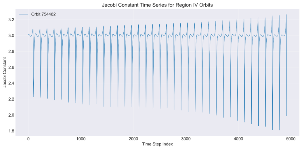
Figure 2.
Poincaré section () of the unique Region IV orbit (ID 754482). 36 crossings indicate weak chaos. Axes are dimensionless in CRTBP units.
Figure 2.
Poincaré section () of the unique Region IV orbit (ID 754482). 36 crossings indicate weak chaos. Axes are dimensionless in CRTBP units.
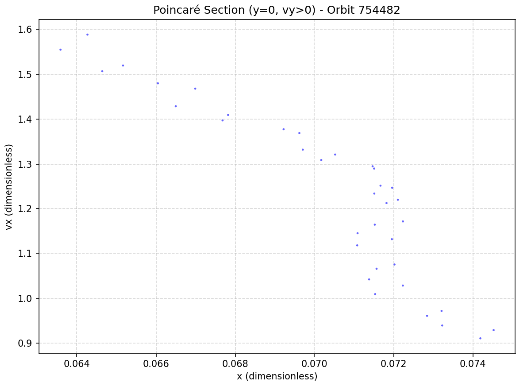
Figure 3.
AUC vs. prefix length K for LSTM+Attention+XGBoost.
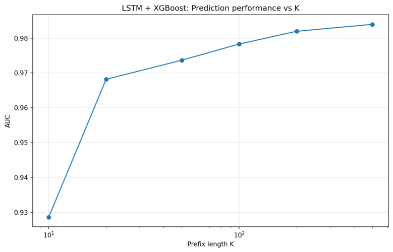
Figure 4.
AUC vs. prefix length K for XGBoost.
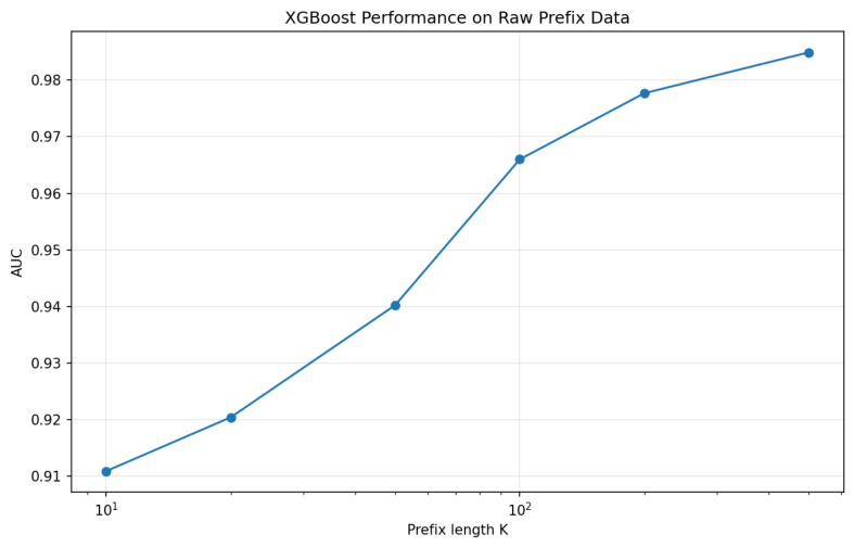
Figure 5.
Example attention weights for Region I and non-Region I orbits (K=500).
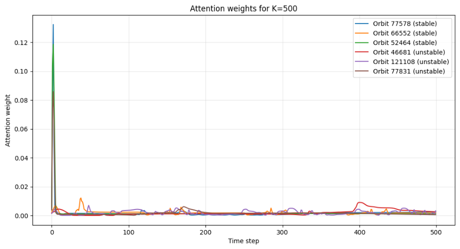
Figure 6.
Top 20 LSTM-encoded feature importances (K=500).
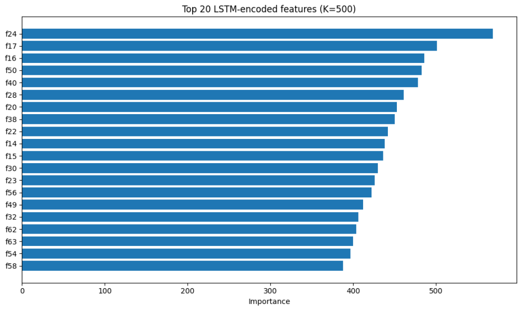
Table 1.
Distribution of one million cislunar orbits across the five classical energy regimes.
| Region | Condition | Number of Orbits | Percentage |
|---|---|---|---|
| Region I | 80,748 | 8.07% | |
| Region II | 0 | 0% | |
| Region III | 2,430 | 0.24% | |
| Region IV | 1 | 0.0001% | |
| Region V | 916,821 | 91.68% |
Table 2.
Test set performance of LSTM+Attention+XGBoost for different prefix lengths K.
| K | Accuracy | Precision | Recall | F1 | AUC |
| 10 | 0.8623 | 0.3625 | 0.8637 | 0.5106 | 0.9286 |
| 20 | 0.9055 | 0.4654 | 0.9131 | 0.6166 | 0.9682 |
| 50 | 0.9148 | 0.4934 | 0.9246 | 0.6434 | 0.9737 |
| 100 | 0.9227 | 0.5198 | 0.9321 | 0.6674 | 0.9783 |
| 200 | 0.9257 | 0.5299 | 0.9479 | 0.6798 | 0.9819 |
| 500 | 0.9322 | 0.5537 | 0.9519 | 0.7001 | 0.9840 |
Table 3.
Test set performance of raw XGBoost (baseline) for different prefix lengths K.
| K | Accuracy | Precision | Recall | F1 | AUC |
| 10 | 0.8386 | 0.3225 | 0.8538 | 0.4681 | 0.9109 |
| 20 | 0.8454 | 0.3334 | 0.8585 | 0.4802 | 0.9204 |
| 50 | 0.8645 | 0.3690 | 0.8849 | 0.5208 | 0.9402 |
| 100 | 0.9029 | 0.4578 | 0.9086 | 0.6089 | 0.9660 |
| 200 | 0.9188 | 0.5063 | 0.9323 | 0.6562 | 0.9777 |
| 500 | 0.9358 | 0.5686 | 0.9473 | 0.7106 | 0.9849 |
Table 5.
Summary statistics of the mean attention weights for each prefix length K. Centroid is normalized by K (in parentheses); peak position is 0-indexed.
Table 5.
Summary statistics of the mean attention weights for each prefix length K. Centroid is normalized by K (in parentheses); peak position is 0-indexed.
| K | Centroid (normalized) | Peak position | Peak value | # local maxima | Top-20% cum. ratio | High-attn intervals |
| 10 | 7.84 (0.784) | 9 | 0.550 | 0 | 0.779 | [9,9] |
| 20 | 16.71 (0.836) | 19 | 0.351 | 0 | 0.797 | [17,19] |
| 50 | 40.85 (0.817) | 49 | 0.147 | 3 | 0.739 | [44,49] |
| 100 | 84.21 (0.842) | 99 | 0.087 | 1 | 0.776 | [88,99] |
| 200 | 168.93 (0.845) | 199 | 0.076 | 97 | 0.762 | [175,199] (sparse) |
| 500 | 195.75 (0.392) | 2 | 0.026 | 30 | 0.393 | [0,32] |
Disclaimer/Publisher’s Note: The statements, opinions and data contained in all publications are solely those of the individual author(s) and contributor(s) and not of MDPI and/or the editor(s). MDPI and/or the editor(s) disclaim responsibility for any injury to people or property resulting from any ideas, methods, instructions or products referred to in the content. |
© 2026 by the authors. Licensee MDPI, Basel, Switzerland. This article is an open access article distributed under the terms and conditions of the Creative Commons Attribution (CC BY) license (http://creativecommons.org/licenses/by/4.0/).
Copyright: This open access article is published under a Creative Commons CC BY 4.0 license, which permit the free download, distribution, and reuse, provided that the author and preprint are cited in any reuse.