

Submitted:
12 August 2026
Posted:
14 August 2026
You are already at the latest version
Abstract
Classical physics describes gravity, electromagnetism, and light with extraordinary precision but not what they are — this paper proposes a unified mechanical model: they are consequences of space being a crystal of spinning spheres. The elements of this crystal — called hyphons (from Greek hyphē, fabric) — are vortices in a superfluid ether, each spinning on one of four tetrahedral axes, packed in the same face-centred cubic (FCC) arrangement as the atoms in a silver crystal. Transverse sound travels through silver at 1,600 m/s — a wave governed by the lattice spacing, stiffness, and density. Light, in this model, is the same kind of wave in the hyphon crystal, governed by the same wave mechanics, travelling at the speed of light. The crystal picture describes undisturbed space; where enough energy concentrates to disrupt the lattice — inside particles and black holes — the underlying superfluid nature of the medium becomes visible. The proton is a vortex configuration in the hyphon lattice with a bound positron in its core giving it charge +1e. The neutron is the same vortex with an additional bound electron cancelling the charge, plus the electron’s pinned half-winding partner — a frozen antineutrino twist — which supplies the neutron’s spin and forces the antineutrino of beta decay. The electron is a wound defect of the lattice’s orientational sector — a localized winding of the spin axes; the free neutrino is a travelling helical wave of the same sector, the space lattice’s chiral acoustic phonon. Every proton and neutron is a vortex that creates a pressure drop propagating through the crystal as a 1/r field — this is gravity. The hyphons carry enormous base energy, but because it is perfectly uniform, only excitations above it are visible as mass. Charge is the winding itself: same-sense windings overlap constructively and repel, opposite windings cancel and attract; the long-range 1/r interaction follows from harmonic relaxation of the lattice — the same Laplace far field as gravity’s pressure deficit — and the electron’s mass is the stored elastic energy of the winding. The strong nuclear force is the overlapping-flow interaction between borderless nucleon vortices in rock salt ordering. The weak nuclear force is the energy threshold for the electron to escape the neutron’s outer well — beta decay; inside nuclei these electrons delocalize between proton cores and bind them. The framework fits the measured proton and neutron form factors with the same exponential distribution family that describes the hydrogen electron — the two organizations of matter separated by the single scale ratio a0/ƛ_p = m_p/(m_e α) ≈ 2.5 × 10⁵ — and reproduces the neutron’s Galster curve as the difference of two dipoles with one free parameter.
Keywords:
superfluid vacuum theory
; ether
; FCC lattice
; topological defect
; wound defect
; emergent monopole
; chiral phonon
; hyphon
; hedron
; emergent gravity
; unified model
; vortex model of matter
; fine structure constant
; electron delocalization
; neutron charge distribution
; rock salt ordering
1. Introduction
Every model in physics is a model — a useful representation of behaviour, not a claim about what the universe ultimately is. The same physical phenomena can often be described accurately by several different models, each illuminating different aspects. Classical physics describes gravity, electromagnetism, and light with extraordinary precision but does not answer what they are. General relativity describes how mass curves spacetime but not what spacetime is. Maxwell’s equations describe fields but not what a field is. The aim of this paper is to explore whether a single mechanical substrate — a lattice of spinning spheres — can reproduce the same observed behaviours through a different and perhaps more intuitive picture. A new model does not invalidate older ones; it offers an additional way to look at the same phenomena.
This paper proposes that space is a crystal of spinning spheres — and that forces, light, and particles are mechanical consequences of this crystal’s structure.
The mechanical-medium picture of space was largely abandoned after Michelson and Morley (1887) found no ether wind, but as Dirac (1951) argued, relativity does not rule out the ether — only a detectable rest frame. In the model below, every measuring instrument is itself a pattern in the lattice, so Lorentz contraction and time dilation emerge as real mechanical effects that cancel any detection attempt (Section 3.4). This work builds on Superfluid Vacuum Theory as developed by Volovik (2003), Zloshchastiev (2011), and others, extending it to a concrete mechanical structure.
Before going into the model itself, a note on confidence levels. The components below are at different stages of development. Higher confidence: the lattice as the medium of space, light as transverse lattice waves (§3), gravity as a vortex pressure gradient (§4), time dilation and gravitational lensing as local lattice properties, and the neutrino as a propagating helical lattice wave — a chiral-phonon-like excitation whose handedness, neutrality, and near-non-interaction follow from a single half-integer winding property (§5.5; its propagation speed and the lattice’s ability to host the half-integer winding remain open). Also higher confidence within §5: electrons and positrons as wound defects of the lattice’s orientational sector, the neutron as a proton with a bound electron and its pinned antineutrino twist, and charge as what these defects are, with measurable probability distributions. Lower confidence: the physical size of the hyphon (the lattice’s existence is well-grounded, but the hyphon’s actual size is not determined by the model — it is only known to be far smaller than the structures built from it), the detailed geometry of the proton vortex, how far it extends into the surrounding lattice, whether it has structure at the atomic scale beyond the nuclear core, and the speculative cosmological extensions in §2.5.3 and §2.6 (origin of matter, cosmological redshift as lattice stretching, and the fate of the lattice). The reader should treat the latter as working hypotheses exploring how the framework might extend, rather than as more settled consequences of the core model.
The most familiar analogue for the proposed structure of space is a metal. Silver has a face-centred cubic (FCC) crystal structure — atoms packed like cannonballs, each touching twelve neighbours. Transverse sound travels through silver at 1,600 m/s, a speed set not by individual atoms but by the lattice’s spacing, stiffness, and density. In this model, light is the same kind of wave in the same kind of lattice, at a much smaller scale.
The model begins with a single substance: the hedron (from Greek hedra, ἕδρα, meaning foundation) — the fundamental particle of the ether, whose size has not been determined. Hedrons organise into hyphons (from Greek hyphē, ὑφή, meaning fabric) — spinning spherical vortices that pack into a face-centred cubic (FCC) lattice. (Whether the hyphon is itself fundamental or, as described here, a vortex in a still-deeper medium is examined in Section 2.2.) Their actual size is not fixed by the model; it is only known to be far smaller than the femtometre-scale charge structure of the nucleon, much as a superfluid healing length is far smaller than the vortices built upon it. All lengths in this paper are therefore given in femtometres rather than in hyphon spacings. Each hyphon spins on one of four tetrahedral axes, like four different orientations of spinning tops in a repeating pattern. This tetrahedral geometry makes the spin-resistance component of the wave response the same in all directions — the flywheel sum over four tetrahedral axes is exactly 8/3 for every propagation direction, a mathematical identity (Section 2.1). Full isotropy requires one further condition: equal radial and tangential bond stiffness (kt/kr = 1), which the vortex tension itself supplies and a direct lattice calculation confirms (Section 3.1); the measured isotropy of the speed of light — parts in 1018 — makes this condition empirically forced.
Calling space a crystal is precise for undisturbed space, but the hyphons are not static atoms — they are vortices in a superfluid. When enough energy concentrates in a region, the crystal lattice breaks down and the fluid nature becomes visible. Consider water in a pool: calm and uniform until someone creates a vortex — a smoke ring or a bubble ring. The vortex is made of the same water but is a distinct structure with its own energy, shape, and persistence. In the hyphon lattice, the proton is such a vortex: a collective circulation pattern whose mass — 938 MeV — is the energy cost of maintaining this circulation above the calm lattice ground state. Neutral pion decay demonstrates this directly: essentially all of its mass radiates away (98.8% to two photons), with no residue left behind — only the pattern’s energy is released (Section 5.2).
The electron is a fundamentally different kind of excitation. Imagine a row of balls packed tightly in a tube: push one extra ball in from the side. It has no room, so it shoves its neighbour, which shoves the next, and a compression pulse travels down the row. The balls themselves barely move, but the disturbance — the pattern — propagates at a speed set by the stiffness of the packing. In crystallography, this is called a crowdion: an extra atom in a close-packed row, travelling as a soliton. Crowdion propagation has been confirmed by molecular dynamics in FCC metals at speeds up to 11 km/s (Shepelev et al., 2023), with kink-mediated mass transfer in Frenkel–Kontorova chains established independently (Marjaneh et al., 2018). Key properties of the crowdion — including relativistic dispersion and two mirror-image forms — correspond to known properties of the electron; Section 5.1 refines the identification — the electron is best described as a wound defect of the lattice’s orientational sector — a localized winding of the spin axes — with the crowdion retained as the motivating analogue.
Particles are built by combining these two kinds of excitations. The proton is a vortex with a bound positron that gives it charge +1e. The neutron is the same vortex with an additional bound electron, cancelling the charge. The structures of the bound states and how they are held together are described in Section 5.2.
Within this framework, all four forces emerge mechanically. Gravity is the 1/r pressure drop a vortex creates around itself; the hyphons carry enormous base energy, but because it is uniform, only the excitations above it appear as mass (Section 4). Light is a transverse wave in the lattice; its speed depends on local pressure, which is why clocks slow and light bends near massive objects (Section 3). Electromagnetism is the overlap interaction of charged defects: same-sign distortion patterns overlap constructively and repel; opposite-sign patterns cancel where they overlap and attract (Section 7). The strong force is surface coupling between nucleon vortices packed in rock salt ordering — bridged by the thin lattice layer between them — with electrons delocalizing between proton cores — the same mechanism as chemical bonding, operating at nuclear distances (Section 6). The weak force is the energy threshold for an electron to escape the neutron’s bound configuration; beta decay is this escape (Section 5.5).
Section 2 describes the structure of space. Section 3 treats light as a lattice wave. Section 4 develops gravity as a pressure gradient. Section 5 describes particle structure: electron, proton, neutron, and their form factors. Section 6 covers nuclear structure and electron delocalization. Section 7 addresses charge and magnetism. Section 8 extends the picture to chemistry.
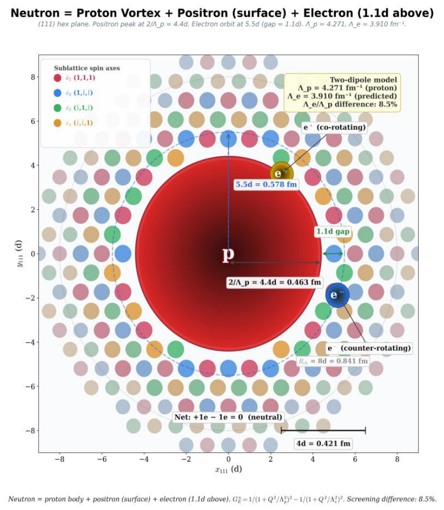
Figure 1.
The neutron as a proton vortex with a bound positron and a bound electron. Cross-section along the hexagonal plane showing the proton’s vortex body (red), the positron’s distribution (gold, R_p ≈ 0.115 fm, 1/Λ_p ≈ 0.236 fm) and the electron’s distribution (blue, R_e ≈ 0.206 fm, 1/Λ_e ≈ 0.251 fm). The surrounding FCC hyphon lattice is colour-coded by sublattice spin axis. Net charge: +1e − 1e = 0 (neutral). Axes and labels in the figure are in units of d ≈ 0.105 fm.
Figure 1.
The neutron as a proton vortex with a bound positron and a bound electron. Cross-section along the hexagonal plane showing the proton’s vortex body (red), the positron’s distribution (gold, R_p ≈ 0.115 fm, 1/Λ_p ≈ 0.236 fm) and the electron’s distribution (blue, R_e ≈ 0.206 fm, 1/Λ_e ≈ 0.251 fm). The surrounding FCC hyphon lattice is colour-coded by sublattice spin axis. Net charge: +1e − 1e = 0 (neutral). Axes and labels in the figure are in units of d ≈ 0.105 fm.
2. Foundation: Structure of Space
2.1. The Ether Lattice
In the proposed model, all physical reality is composed of a single substance: a superfluid ether. The fundamental particle of this framework is the hedron (from Greek hedra, ἕδρα, meaning foundation; symbol η), the base unit of ether whose size has not been determined. Hedrons organise into hyphons (from Greek hyphē, ὑφή, meaning fabric; symbol υ)—near-spherical spinning structures whose size is not fixed by the model, each spinning on a single axis. These hyphons form the fabric of space, arranged in a face-centred cubic (FCC) lattice—the same crystal structure as copper or aluminium, and the densest possible packing of equal spheres. The FCC unit cell contains four elements, each belonging to a different sublattice. The four sublattice spin axes point along the four directions of a regular tetrahedron: (1,1,1), (1,−1,−1), (−1,1,−1), and (−1,−1,1), normalised. A spinning element resists impulses perpendicular to its spin axis (flywheel effect) but not along it. For any direction of impulse, the total flywheel resistance from the four sublattices sums to exactly 8/3—a constant, independent of direction. This is a mathematical identity of the regular tetrahedron (a spherical 2-design) and makes the flywheel component of the wave response isotropic without fine-tuning; the elastic (bond) component becomes isotropic under the same tension condition — equal radial and tangential bond stiffness — established in Section 3.1. The hyphon size corresponds to the healing length of the superfluid—the characteristic scale at which the medium recovers from a disturbance, directly analogous to the healing length in superfluid helium-4 (whose vortex core is of order 1 Å). As in helium-4, this length is a real physical property of the medium, but its numerical value is not determined within the present model.
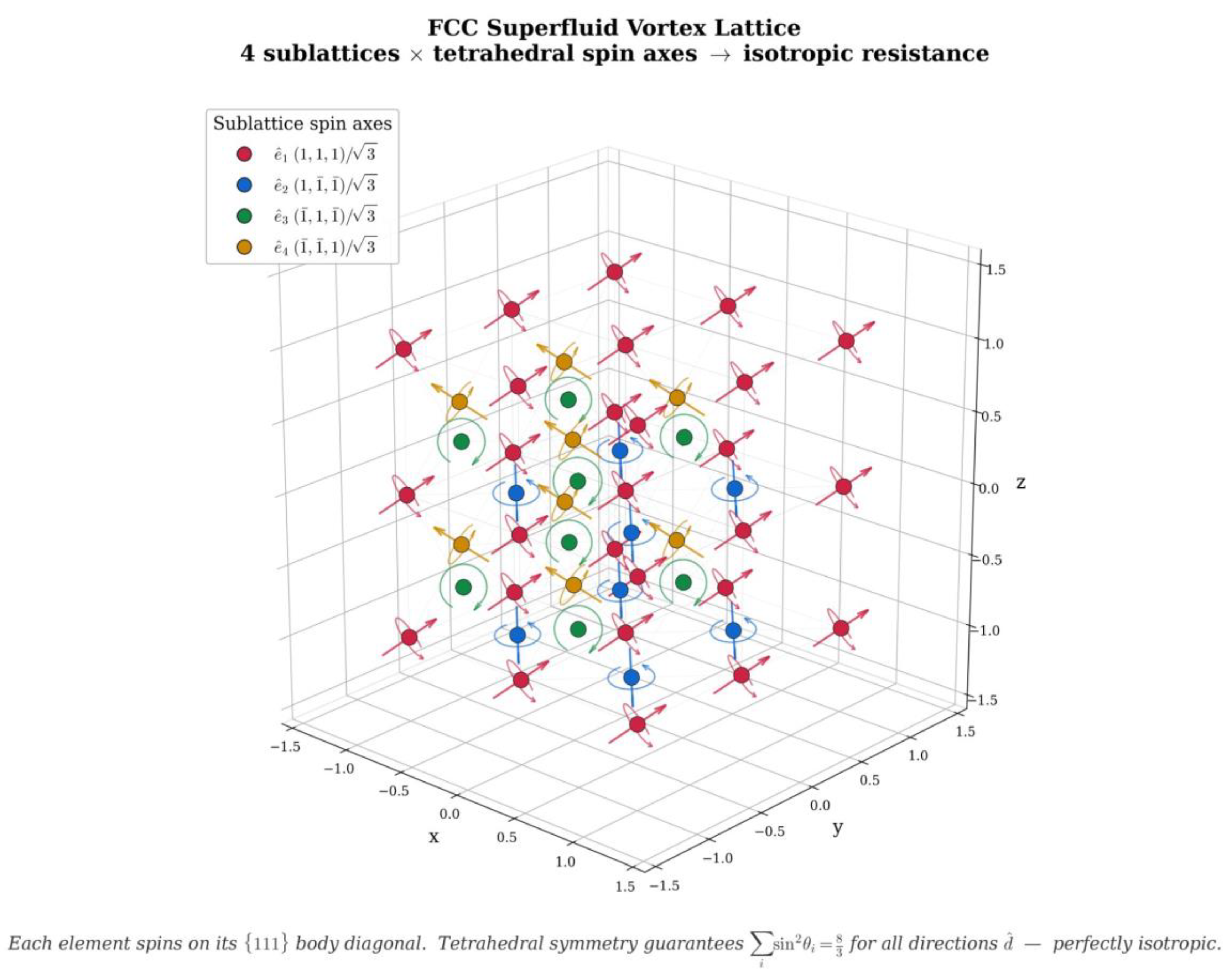
Figure 2.
The FCC superfluid vortex lattice. Each hyphon (sphere) spins on its local tetrahedral axis, colour-coded by sublattice: ê1 (red, (1,1,1)/√3), ê2 (blue, (1,−1,−1)/√3), ê3 (green, (−1,1,−1)/√3), ê4 (gold, (−1,−1,1)/√3). Arrows indicate spin axis orientation. The tetrahedral symmetry guarantees Σ sin2θᵢ = 8/3 for all impulse directions—perfectly isotropic flywheel resistance.
Figure 2.
The FCC superfluid vortex lattice. Each hyphon (sphere) spins on its local tetrahedral axis, colour-coded by sublattice: ê1 (red, (1,1,1)/√3), ê2 (blue, (1,−1,−1)/√3), ê3 (green, (−1,1,−1)/√3), ê4 (gold, (−1,−1,1)/√3). Arrows indicate spin axis orientation. The tetrahedral symmetry guarantees Σ sin2θᵢ = 8/3 for all impulse directions—perfectly isotropic flywheel resistance.
The structure of space described here is a supersolid: a coherent quantum medium that is simultaneously crystalline and superfluid. The closest physical analogue is superfluid helium-3, a fermionic superfluid whose order parameter itself carries spin and orbital structure — far nearer to a medium of spinning elements with oriented axes than a scalar fluid — and the system on which the superfluid-vacuum lineage of this work (Sinha et al., 1976; Volovik, 2003) is built. Both superfluid and crystalline characters coexist: the lattice is a self-organised density pattern of the underlying medium, and topological defects of this pattern (vortices, wound defects) propagate without requiring hyphon creation or destruction. The FCC arrangement itself arises from the dense packing of the elements — equal repulsive spheres adopt this packing on their own (Section 2.2) — while the gyroscopic spin coupling between neighbours governs the medium’s wave properties rather than selecting the lattice: the four-sublattice tetrahedral spin geometry is what renders the spin response of the collective wave excitations isotropic. Those excitations — what would be sound modes in a laboratory supersolid — are, in the hyphon lattice, light.
Each hyphon has twelve nearest neighbours arranged in a cuboctahedron—the coordination geometry of FCC. Adjacent elements belong to different sublattices and spin on axes 109.5° apart. The hyphon size is set by lattice pressure: higher pressure compresses the hyphons into smaller, stiffer vortices, raising the speed of light; lower pressure allows them to expand and soften, lowering it. This is the same physics observed in superfluid helium-4, where the quantised vortex core diameter shrinks under pressure and expands at low pressure — at sufficiently negative pressure (−6.9 bar) the core expands without limit and the vortex ceases to exist (Maris, 1994). Far from mass, lattice pressure is high, the hyphons are maximally compressed, and the speed of light approaches an asymptotic ceiling. Near mass, the pressure drops, hyphons expand, and the local speed of light decreases. The same bridging mechanism operates at larger scales — nuclear binding (Section 6.1) is mediated by the hyphon lattice between neighbouring nucleon cores in rock salt ordering, whose borderless flow fields overlap throughout.
2.2. Substrate and Structure: Options Considered
The model makes three structural choices, each with alternatives that were weighed rather than assumed. They are set out here so that the basis for each selection is explicit.
Why a solid. The medium must be a solid — crystalline or amorphous — and cannot be a gas or ordinary liquid. The reason is that both gravity and charge are represented as static 1/r fields (Section 4 and Section 7), and only a solid possesses static shear rigidity, the property required to sustain a static field without it relaxing away. A gas or liquid has zero static shear modulus and cannot hold such a field. This requirement is firm; the remaining choices concern which kind of solid and what it is built from.
Crystalline versus amorphous. Equal repulsive spheres organise themselves without any attractive force: compacted slowly they form a face-centred-cubic crystal (the densest packing, and the entropically favoured equilibrium state), while compacted rapidly they jam into an amorphous glass (metastable). Both reproduce the observed isotropy of light, but by different routes — the amorphous solid washes out any preferred direction by disorder, whereas the FCC crystal achieves the isotropy of its spin response by construction — its four tetrahedral sublattice spin-axes form a spherical 2-design (Σ sin2θ = 8/3) — with its elastic response isotropic under the tension condition of Section 3.1. For the wave physics the two are effectively indistinguishable: in a disordered medium only long-wavelength waves propagate coherently, and the scattering from sub-femtometre disorder is negligible over any observable distance. The crystalline arrangement is adopted as primary on formation grounds — it is the equilibrium state, and slow formation yields it — while recording that an amorphous medium would give the same gravity, the same charge behaviour, and the same wave propagation. The structure is therefore not forced by observation; it is selected on grounds of formation and equilibrium.
Balls versus vortices. The hyphons may be either fundamental spinning balls (with no deeper structure) or spinning vortices in a deeper continuous medium (the hedron ether). The fundamental-ball picture is the simpler ontology and closes the mechanics at one level. The vortex picture requires a deeper medium, which would carry its own compression wave; this is not an objection, since a single medium routinely carries several wave modes at different speeds simultaneously (superfluid helium supports first, second, and fourth sound together with slow Tkachenko vortex-lattice waves), and such a mode need not be observable at our scale. The two pictures are equivalent for most of the model, with one exception that bears on the wave sector: only the vortex picture supplies, through the inward pressure-pull of each vortex, the standing shear tension that makes the longitudinal and transverse wave speeds equal (Section 3.1). A lattice of passive balls settles at its potential minimum, where the shear stiffness vanishes and the speeds are unequal; a vortex lattice sits under self-generated tension, where the shear stiffness is non-zero. The empirical weight behind this consideration is isotropy: the same standing tension sets the radial and tangential bond stiffnesses equal — the condition under which the lattice’s elastic response, and with it the speed of light, becomes exactly direction-independent (Section 3.1), as observation requires to parts in 1018 — and equal longitudinal and transverse speeds follow from the same condition. The spinning-vortex substrate additionally supplies the orbital-and-spin structure that the helical neutrino mode of Section 5.5 requires. Both considerations favour the vortex picture. Both are retained, with the vortex picture preferred where the wave sector is concerned and the ball picture noted as the simpler alternative.
A supersolid, rigid fast and fluid slow. Whichever substrate is chosen, the medium is a supersolid: crystalline and superfluid at once. It is not frozen rigid — it retains the fluid degrees of freedom that allow vortices, and hence matter, to exist, since circulation cannot persist in a perfectly rigid solid. The reconciliation of this fluid flow with the rigidity that carries waves comes from the gyroscopic character of the spinning elements: a spinning body resists rapid disturbances stiffly but yields to slow ones. The medium is therefore rigid at the high frequencies of light — supplying the shear stiffness that carries the transverse wave — while remaining fluid at low frequency, where vortices form and move. The static 1/r fields of gravity and charge (Section 4 and Section 7) are indifferent to this distinction: a static 1/r field is the ordinary point-source solution in any medium with non-zero static shear, and is held equally well whether the medium is stiff or soft. The open question is confined to the wave sector: whether the high-frequency gyroscopic stiffening makes the longitudinal and transverse speeds equal (v_L = v_T), rather than merely strong but unequal, as examined in Section 3.1.
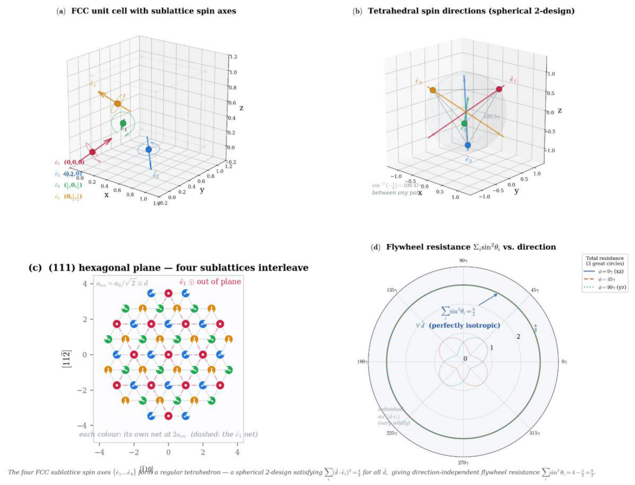
Figure 3.
FCC lattice geometry in detail. (a) The FCC unit cell with four subhyphons and their spin axes. (b) The four tetrahedral spin directions, separated by 109.5°, forming a spherical 2-design. (c) A (111) hexagonal plane — the close-packed triangular layer. All four sublattices interleave within it, each forming its own sparser triangular net; the ê1 spins point out of the plane (coins lying flat) while the other three axes lie close to it. (d) Polar plot of total flywheel resistance versus impulse direction: the sum Σ sin2θᵢ = 8/3 is constant for all directions (green circle), even though each sublattice’s individual contribution varies wildly. Distances are quoted in the ruler unit d of Section 2.3, which is a bookkeeping scale rather than a measured hyphon size; the physical spacing is unknown and the value is fixed only for consistency across figures.
Figure 3.
FCC lattice geometry in detail. (a) The FCC unit cell with four subhyphons and their spin axes. (b) The four tetrahedral spin directions, separated by 109.5°, forming a spherical 2-design. (c) A (111) hexagonal plane — the close-packed triangular layer. All four sublattices interleave within it, each forming its own sparser triangular net; the ê1 spins point out of the plane (coins lying flat) while the other three axes lie close to it. (d) Polar plot of total flywheel resistance versus impulse direction: the sum Σ sin2θᵢ = 8/3 is constant for all directions (green circle), even though each sublattice’s individual contribution varies wildly. Distances are quoted in the ruler unit d of Section 2.3, which is a bookkeeping scale rather than a measured hyphon size; the physical spacing is unknown and the value is fixed only for consistency across figures.
The closest laboratory analogue to the hyphon lattice is the quantised vortex lattice in rotating superfluid helium-4 (Feynman, 1955; Yarmchuk, Gordon & Packard, 1979): identical vortex elements arranged in a regular triangular grid, each with fixed quantised circulation and fixed core size. Viewed along a body diagonal, the hyphon FCC lattice has the same triangular cross-section. In both systems, the medium itself (helium-4 atoms or hedrons) is something deeper — the vortices are organised structures within that medium. The individual vortex tubes in the He-4 grid are the analogue of hyphons — the lattice elements. Larger vortex rings that move through this lattice correspond to particles moving through the hyphon lattice — coherent movement patterns travelling between the vortex tubes without destroying them. The critical rotation rate Ωc2, at which vortex cores overlap and the lattice is destroyed, corresponds instead to black hole formation in the hyphon lattice (Section 2.5). The estimated He-4 vortex core rotation speed is approximately 0.7 times the speed of sound in helium — individual vortices spin below the wave speed, yet the lattice collectively transmits sound at the full wave speed. This grounds the assumption that hyphons spinning below c collectively transmit light at exactly c.
The hyphons carry energy—every vortex is a circulating structure, and circulation is kinetic energy. The undisturbed lattice therefore has an enormous energy density. However, this energy is perfectly uniform throughout free space. Because gravity in this model arises from lattice pressure gradients (see Section 4), not from absolute energy density, a uniform background produces no gravitational effect and no observable mass.
Two mechanisms break down the lattice: inside black holes, where the extreme concentration of vortex energy overwhelms the lattice (see Section 2.5); and beyond the observable universe, where the hedron fluid has not yet accumulated enough energy to crystallise into a lattice (see Section 2.6). Between galaxies the lattice persists — light demonstrably crosses intergalactic space — though toward galaxy edges it may thin toward its stability limit, a possibility taken up in Section 2.6.
2.3. Energy States of the Ether
The ether exists in four states, distinguished by how much structure — and therefore energy — is present. Each transition toward greater order requires energy; destroying structure releases it.
At the lowest energy, the ether is an unstructured hedron fluid — disordered, with no lattice, no light, no matter. When sufficient energy is available, hedrons crystallise into hyphons — spinning spheres arranged in the FCC lattice. This crystallisation stores energy in the aligned structure: the ordered state is a higher-energy configuration, maintained by the spin coupling between neighbours. The spin creates the flywheel coupling that transmits impulses at c.
Within the lattice, further structure is possible. A proton is a coherent toroidal vortex pattern in the hyphon lattice — an excitation above the ground state whose energy IS the proton mass (938 MeV). Hyphons do not flow with the proton; they reorganize at the leading edge of the pattern and relax back at the trailing edge as it translates. Destroying a proton releases the pattern’s stored energy back into the lattice, as demonstrated by π0 decay, where essentially all of the mass radiates away as photons. The electron is a different kind of excitation — a localized topological defect that travels through the lattice (see Section 5.1).
At the extreme, a black hole forms: the most energetic vortex structure, whose concentrated energy overwhelms the lattice entirely. Inside a black hole the FCC lattice has melted to unstructured hedron fluid, which is the only regime in this hierarchy where actual bulk fluid flow occurs — outside black holes, “circulation” is pattern translation through hyphons that remain close to their lattice sites (see Section 2.5).
Each transition is reversible: add energy and structure builds upward; let energy radiate away and structure dissolves downward.
2.4. The Hyphon
The hyphon’s physical size is not determined by the model. Like the vortex-core size in superfluid helium-4 — of order 1 Å, set by the medium’s healing length rather than by any external scale — the hyphon has a definite size in principle, but fixing its value would require independent knowledge of the medium’s stiffness that is not yet available. All that is required for the rest of this paper is that the hyphon is far smaller than the femtometre-scale charge structure of the nucleon. Lengths are therefore quoted in femtometres throughout. A note on the figures: several diagrams mark lengths in the unit d ≡ ℏ/(2mₚ c) ≈ 0.105 fm, a convenient nuclear-scale ruler set by the proton’s Compton scale. This is a unit of length only, not a claim about the hyphon’s actual size; values can be read directly in femtometres using d ≈ 0.105 fm (for example, 8d ≈ 0.841 fm).
Every hyphon carries rotational energy from its spinning structure. This energy is completely invisible — it is the uniform background against which all measurements are made. What we observe as “mass” is the excitation energy of vortex structures above this background — the circulation energy of the pattern, not the hyphons themselves.
The proton mass is the excitation energy of the proton vortex above the lattice ground state (Section 5.2); it is not expressed here as an integer count of hyphon masses, since the hyphon mass is not independently fixed.
This offers a route to the vacuum energy problem — by departing from general relativity on one point. In general relativity all stress-energy gravitates, including a uniform vacuum energy; combining this with quantum field theory’s vacuum energy estimate overshoots the observed value by some 10120. In this model, gravity couples to pressure gradients rather than to absolute energy density, so the enormous uniform background produces no gravitational effect by construction. This is a modification of general relativity proposed as a feature, not a resolution within it; on this reading, the cosmological constant measures residual non-uniformity at cosmic scales, not the total energy.
2.5. Black Holes
2.5.1. Structure and the Event Horizon
A black hole is a giant vortex in the superfluid ether — the same structure as a proton, scaled up until the concentrated energy overwhelms the lattice. The Schwarzschild radius r_s = 2GM/c2 marks the shell where the hyphons expand beyond their stability limit and cease to exist as vortices — directly analogous to superfluid He-4 vortex cores at negative pressure, which expand without limit at −6.9 bar (Maris, 1994). A black hole is black not because light is too slow to escape, but because there is no lattice left to carry it.
Inside the event horizon lies unstructured ether — carrying the full rotational energy of everything that fell in, but with no structure to propagate it outward or concentrate it inward. General relativity predicts a singularity; the ether model has a pressure floor at zero. The energy disperses into the unstructured interior. The central singularity of general relativity is replaced by a finite-density fluid interior; the only sharp surface in this model is the horizon shell where the lattice ends, not a central point of infinite density.
This boundary marks a regime change in the underlying fluid dynamics. Outside the event horizon, the FCC lattice is intact: hyphons remain close to their lattice sites and carry vortex patterns through the medium without bulk transport, so particle structures are pattern excitations rather than circulating fluid. Inside the horizon, the lattice has melted to unstructured hedron fluid, and the standard fluid-dynamic picture resumes — bulk circulation is now possible, and the classical Landau critical velocity criterion (Landau, 1941) directly limits how fast the interior fluid can flow before its excitation spectrum renders the configuration unstable. The lattice-to-fluid transition is therefore not just a structural change; it is a change in which conservation laws and stability conditions apply.
2.5.2. Radiation and Evaporation
A black hole radiates because the boundary between structured lattice and unstructured interior is not static — it is a contact surface where the rotational energy of the interior meets the lattice ground state. The energy mismatch drives continuous energy transfer outward into the lattice. No quantum mechanics is required — no virtual particle pairs, no tunnelling — only the mechanical coupling between unstructured ether and the lattice at their shared boundary. Smaller black holes have tighter curvature, steeper energy gradients, and radiate faster — the same direction as the standard prediction (Hawking temperature ∝ 1/M, radiated power ∝ 1/M2); whether this mechanical mechanism reproduces the quantitative law is open.
When mass falls into a black hole, more lattice is overwhelmed and the event horizon creeps outward — the infalling energy adds to the vortex concentration. Without infalling matter to sustain it, the black hole slowly radiates its stored energy outward: the event horizon contracts, and eventually the energy drops below the threshold at which particles can re-form. The cascade reverses: the radiated energy reconstitutes lattice → particles. The black hole evaporates into ordinary matter.
2.5.3. Black Hole Collisions and the Origin of Matter
The remainder of this subsection is speculative — a sketched mechanism rather than a worked-out derivation, included because the framework points naturally toward it.
In the undisturbed lattice, creating a vortex ring with winding number +1 (a proton) forces the simultaneous creation of a ring with winding number −1 (an antiproton). This is not an imposed rule but a consequence of three properties of the medium: the lattice has no external boundaries, circulation is quantised, and total circulation is conserved. The opposite winding cannot be absorbed by walls (none exist), cannot spread diffusely (quantisation forbids it), and must exist (conservation requires it). It is therefore forced to concentrate into another ring — this is pair production. A laboratory analogue of this forced pairing exists: in spinor polariton condensates, an effective field splits an integer soliton into two half-solitons of opposite texture charge, which the field then separates (Hivet et al., 2012).
Black hole collisions are the one environment where this constraint is relaxed. The interior of a black hole, in this model, is melted lattice — unstructured ether with no vortex order and no quantised circulation (Section 2.5.1). The boundary between intact lattice and melted interior functions as an absorbing wall: opposite circulation can pass into the melt without forming a quantised vortex ring.
When two black holes collide, the lattice between and around them is violently destroyed and subsequently refreezes outward from the cooling boundary of the merged remnant. During this refreezing, vortex rings nucleate in the re-crystallising lattice. The collision geometry is not symmetric — the two black holes differ in mass, spin, and approach trajectory — and the refreezing boundary conditions reflect this asymmetry. If slightly more +1 winding nucleates in the lattice than −1, the deficit is absorbed into the melted interior of the merged black hole.
The net result: the re-frozen lattice contains more protons than antiprotons, and the merged black hole stores the corresponding negative winding in its structureless interior. The total winding of the universe remains exactly zero. No fundamental matter–antimatter asymmetry of physical law is required. Which winding sign ended up in the lattice was determined by the accident of the initial collision geometry. We call that sign “matter.” Had the collision tilted the other way, the lattice would contain what we now call antiprotons and positrons, and we would call those “matter” instead.
2.6. The Observable Universe
In superfluid helium-4, the vortex state exists only within a specific pressure and temperature window. The ether lattice has analogous bounds. Lattice formation requires sufficient energy density — the hedron fluid must accumulate enough energy for spin alignment to crystallise. The observable universe is the region that has crystallised so far. Beyond its boundary lies the unstructured hedron fluid — not empty but featureless, carrying less energy per volume than the structured space we inhabit. No light propagates there because no lattice means no transverse waves — directly analogous to molten aluminium, which carries no transverse sound while the solid FCC crystal carries it at 3100 m/s.
At galaxy edges, far from the cumulative pressure contributions of surrounding matter, the lattice may thin toward its stability limit — the healing length grows, hyphons stretch apart, and the mechanical properties change. The anomalous flattening of galaxy rotation curves — conventionally attributed to dark matter — may instead reflect this lattice thinning: as the lattice stretches, the gravitational coupling deviates from the simple 1/r2 prediction derived for a uniform lattice. Where the lattice fails entirely, the ether reverts to its unstructured state — directly analogous to superfluid helium-4 below the critical rotation rate Ωc1, where no vortices form and the fluid remains featureless. Any such reading must eventually confront the evidence that gravitational lensing tracks mass displaced from the visible baryons (the Bullet Cluster) and that the acoustic peaks of the cosmic microwave background independently require a non-baryonic component; these remain open hurdles for a thinning-based account.
The remainder of this section is speculative — an extension of the framework into cosmology. If the lattice is a real medium, several otherwise puzzling cosmological facts have a mechanical reading. Cosmological redshift, in standard general relativity, is energy that simply vanishes as the universe expands — a consequence of energy conservation not holding globally in an expanding spacetime. In the lattice picture, the lattice is physical and stretches as the universe expands; the lost photon energy goes into the elastic state of the stretched lattice. Energy conservation is restored because the medium is real. This is distinct from frictional dissipation: pure dissipation would distort the cosmic microwave background’s blackbody spectrum (which it does not), and the (1+z) time dilation observed in distant supernovae cannot be produced by friction — it requires actual expansion of the medium.
Within this picture, the Big Bang is retained as a real event but demoted from a unique cosmic origin to a local one. The evidence — redshift increasing with distance, the CMB, an apparent point-like origin — is real and best explained by a concentrated initial energy source. But that source need not be the origin of everything. A collision between two very large black holes, or between universe-scale dense regions of the surrounding ether, would produce exactly what we observe: a roughly point-like initial concentration, outward expansion, lattice formation as density drops into its stability window, and matter formation where density exceeds the matter threshold. No singularity is required, and no inflationary epoch. “The” Big Bang becomes our Big Bang — a local collision event, structurally analogous at multiverse scale to the galaxy collisions we observe at the scale below. What this sketch does not yet supply is what inflation was introduced for: the near-uniformity of the microwave background across causally disconnected regions, its nearly scale-invariant fluctuation spectrum, and spatial flatness. A collision origin must eventually account for these; that accounting has not been attempted here.
This picture is naturally scale-invariant. Dense regions nest inside sparser ones at every scale we can observe: planets in solar systems, solar systems in galaxies, galaxies in clusters, clusters in the cosmic web. A locally dense patch of ordered lattice — what we call our universe — is simply the next step in this hierarchy. Other patches may exist outside our horizon, separated from us by regions of unstructured ether. They are invisible to us not because of expansion alone, but because no transverse wave can cross unstructured ether: between two patches of lattice the light has nowhere to travel. Invisibility does not mean isolation, however: the unstructured fluid between patches still carries pressure and bulk flow, so energy can pass where light cannot — the patches are optically decoupled but thermodynamically coupled, through different channels of the same medium. The word “multiverse” here carries no exotic implication; it just means the neighbourhood at the next scale up.
The fate of the lattice in this picture is set by the ether outside our patch. If the surrounding density is similar or higher, our expansion eventually slows or reverses and the lattice is preserved. If much lower, our lattice stretches thinner until it falls below its stability threshold and dissolves from the edges inward. This is heat death in a stronger form than the standard one: not merely cold matter in cold space, but loss of structured space itself — the lattice ceases to exist, and with it the medium that carries light, particles, and time. Each patch, moreover, stores energy only within its lattice’s stability window: the spinning hyphons hold energy up to the melting threshold (Section 2.5), and the lattice dissolves below the formation threshold, so patches generically differ in energy density, and energy flows between them through the boundary fluid wherever a neighbour is below saturation. The cosmological constant, in this framework, may not be fundamental: a small positive Λ corresponds to our neighbourhood being slightly less energy-dense than our interior, producing outward pressure — and, since the exchange is ongoing, Λ on this reading need not be strictly constant in time. This interpretation is appealing but not yet worked out quantitatively.
3. Light as a Lattice Wave
Light is a propagating wave in the ether lattice. It is not a particle. It is a transverse wave propagating through the lattice at the speed of light. Its energy is determined by its frequency—from radio waves to gamma rays.
This identification is not an analogy. In solid state physics, quantised lattice vibrations are called phonons. Their energy is E = ℏω, they obey Bose-Einstein statistics, and their propagation speed is the speed of sound in the medium—a material property. Photons obey the same energy relation (E = ℏω), the same statistics, and propagate at c—the speed of sound in the ether lattice. The quantum field theory formalism (creation and annihilation operators, Fock space) is identical for both. Phonons are quantised because the underlying oscillators obey quantum mechanics; the crystal’s discreteness supplies instead the dispersion and the high-frequency cutoff. The same division applies here. The natural first guess is that quantisation enters at the source — emitters have discrete states, so energy leaves in lumps — but single-photon experiments show the lump remains indivisible in flight, so the quantum of action must also govern propagation; supplying its origin is an open question of this framework, faced rather than assumed. The speed of light c = 1/√(ε0μ0) has the same mathematical structure as the speed of sound v = √(K/ρ), with the permittivity ε0 playing the role of lattice compliance and the permeability μ0 playing the role of inertial density. The electric and magnetic force constants were established independently—from electrostatic and magnetostatic experiments respectively—before Maxwell (1865) showed that their combination gives the speed of light. Three independent experiments, three separate phenomena, one number. If the ether lattice is discrete, a Debye-like cutoff should exist: a maximum photon frequency at which the wavelength equals twice the lattice spacing, above which electromagnetic waves cannot propagate.
3.1. Transverse and Longitudinal Modes
The hyphon lattice supports both transverse and longitudinal wave modes. Because the hyphon–hyphon coupling is gyroscopic rather than purely central-force, the Cauchy relation that fixes v_L ≈ √3·v_T in an isotropic central-force solid (Poisson ratio ¼) need not apply. The tetrahedral spin sum Σᵢ sin2θᵢ = 8/3, identical for every direction, makes the gyroscopic part of the response isotropic. Isotropy of the elastic part, and equality of the longitudinal and transverse speeds, are distinct further conditions — and both, it turns out, follow from the single stiffness condition k_t/k_r = 1 derived below. Equal speeds require instead that the medium’s transverse (shear) stiffness be comparable to its compression stiffness (k_t/k_r ≈ 1). A direct gyroscopic (velocity-dependent) coupling does not supply this — it splits the two branches and renders one anomalously slow. A genuine shear stiffness does, and in this model the natural source is the standing inward tension of the vortex lattice: a bond held under tension T has transverse stiffness k_t = T/r0, and if the inward pull falls as 1/r (the same dependence invoked for gravity, Section 4), then k_t/k_r = 1 and v_L = v_T follows. A direct harmonic calculation of the FCC nearest-neighbour lattice confirms this: with bond force-constant matrix Φ = k_r n̂n̂ᵀ + k_t(I − n̂n̂ᵀ), setting k_t/k_r = 1 renders all three acoustic branches exactly degenerate at every wavevector and isotropic at leading order, with a stable spectrum; at k_t = 0 the calculation recovers the textbook central-force results (v_L/v_T = √2 along 100, transverse speeds varying by roughly 30% with direction). Because a single vortex pull is short-ranged rather than exactly 1/r, this equality is expected to hold to good approximation in the dense-packing limit (lattice spacing ≈ core size) rather than as an exact identity; a small residual v_L ≠ v_T remains possible and is not observationally excluded. Establishing k_t/k_r = 1 rigorously from the vortex tension — the condition that delivers both exact isotropy (empirically required to parts in 1018) and equal mode speeds — remains the central open problem of the wave sector.
Which mode is excited depends on the source geometry. Two well-documented excitation types in normal crystals illustrate the distinction. A normal-incidence piezoelectric transducer pressed against the surface of a steel block launches a pure longitudinal compression wave — the pulse propagates as a sequence of compressions and rarefactions along its travel direction. A Y-cut quartz transducer pressed against the same block launches a pure transverse shear wave — the pulse propagates as side-to-side particle motion perpendicular to its travel direction. Once propagating in the undisturbed bulk, the two modes do not convert into each other.
The same rule applies in the hyphon lattice. A rotational source — an accelerating charge — generates motion perpendicular to the outgoing wave direction and excites transverse modes; this is light. A radial source — the one-time lattice rearrangement when a charge configuration changes — generates motion along the outgoing wave direction and excites longitudinal modes; in this model these serve as the field-establishment channel (Section 4 and Section 7.1) rather than as an observed radiation. The displacement modes do not exhaust the lattice’s wave families: because the lattice elements spin, branches also exist in which the elements’ rotation participates — the established precedents are spin waves in magnetic crystals (pure orientation) and chiral phonons (displacement circling with locked handedness). The neutrino, formerly identified with the longitudinal mode, is reassigned to a handed member of this rotational family (Section 5.5); which branch of the decorated lattice carries it is an open realisation question.
3.2. Emission and Absorption
When a lattice impulse (light wave) reaches an electron, it transfers energy to the electron. The electron — a localized lattice defect strongly coupled to the medium — absorbs energy from the impulse. This energy changes the electron’s speed and orbit. The reverse process—an electron dropping to a lower energy state—releases energy back into the lattice as an impulse that propagates away as a wave at the speed of light.
Atomic energy levels cannot be set by the space lattice alone: measured levels differ from element to element, scale with nuclear charge, and shift with nuclear mass (the hydrogen–deuterium isotope shift), so they depend on the nucleus, not on a universal lattice ladder. In this model the quantisation of bound states arises instead as an orbit-closure condition: the electron defect circulating in a nucleus’s field must close its path coherently, and only discrete orbits do so — reproducing the structure of the dependence (on charge and on reduced mass), though not yet derived quantitatively. The Peierls–Nabarro barrier — the physics that quantises crowdion velocities in FCC metals (Section 5.1.2) — remains relevant to the free defect’s preferred translation speeds, but it is not the origin of atomic spectra.
Light appears quantised at emission and detection because the electron is a discrete object that exchanges energy in steps. Between them the disturbance propagates as a lattice wave — yet single-photon experiments (anticorrelation at a beamsplitter) show the travelling quantum is indivisible in flight, so the wave must carry its lump character with it rather than acquiring it only at the detector. No point particle traverses space; the “photon” is one quantum of energy carried by a lattice wave whose integrity in transit is part of the open quantisation question (Section 3).
The speed of light depends on the local lattice pressure—higher pressure yields faster propagation. This has directly measurable consequences (see Section 4.2).
3.3. Bell’s Inequality and Lattice Waves
Bell (1964) proved that no theory in which particles carry predetermined values can produce correlations exceeding a certain bound. The CHSH formulation (Clauser et al., 1969) sets this bound at 2. Quantum experiments yield scores up to 2√2 ≈ 2.83, violating this bound. This result has been widely interpreted as proof that nature is non-local—that measurement of one particle instantaneously affects a distant partner.
In the present model, light is not a particle carrying predetermined values—it is an impulse propagating through a continuous lattice. Two photons emitted from a common source (such as electron–positron annihilation) are correlated lattice waves sharing a common origin. Their phases, polarisations, and angular momenta are established at the moment of creation and carried independently through the lattice. Conservation laws guarantee that measuring one wave’s properties constrains the other’s—no signal needs to travel between them.
Whether correlated lattice waves in the FCC structure can quantitatively reproduce the 2√2 violation of the CHSH bound has not been demonstrated. Bell’s theorem was derived for point particles with hidden variables, not for extended waves in a discrete medium, and it is not obvious that its assumptions map onto the lattice model. A rigorous derivation of CHSH correlations from FCC lattice wave mechanics is an open problem. Until it is completed, the model’s compatibility with Bell test results remains unresolved.
3.4. Light in Matter and the Michelson–Morley Experiment
In matter, light drives the bound electrons into oscillation, and their coherent re-radiation interferes with the incoming wave: in the forward direction the superposition is phase-delayed — this is refraction — while sideways the contributions cancel: the phase-locked electrons form, in effect, a phased array aimed forward by the wave itself, and where the cancellation is incomplete because the medium is dilute or non-uniform, the residue is precisely the observed Rayleigh scattering of the sky and the whiteness of droplet media. The effective speed is set by this driven re-radiation, not by a per-electron delay — nothing in the medium travels below the lattice wave speed; the accumulated phase lag is equivalent to extra optical path, which is why the product n·d is called the optical path length — and the speed does not decrease monotonically with electron density (diamond, denser in electrons than many opaque materials, is transparent). Metals are opaque for a different reason: their free electrons respond collectively, and below the plasma frequency this response excludes the wave — above it, thin metals become transparent again, as alkali metals do in the ultraviolet.
The Michelson–Morley experiment (1887) found no variation in the speed of light with direction. In this model, the explanation is fundamental: particles are patterns in the hyphon lattice, not objects moving through it. A pattern moving through the lattice physically contracts in the direction of motion and its internal processes physically slow down — Lorentz contraction and time dilation are real mechanical effects, not coordinate artefacts. These effects exactly cancel any attempt to measure the pattern’s motion through the lattice. This is what Lorentz proposed in 1892. Einstein’s special relativity (1905) gives identical predictions. In this model, Lorentz invariance is not postulated — it emerges automatically because every measuring instrument is itself a pattern in the same medium it is trying to measure. A moving medium supplies a further test of this mechanism. Fizeau (1851) measured the speed of light in flowing water and found partial drag: the flow carries the light along, but only by the fraction (1 − 1/n2) of the water’s own speed. This is exactly what the driven re-radiation picture requires of a static lattice: the wave in the medium is a superposition of two parts existing together — the lattice part, carried by the ether, which does not move, and the part continuously radiated by the driven charges as they oscillate in step with the passing wave (no capture, no delay — the same phase-locked emission that produces refraction above); since those charges move with the water, their contribution is convected with it. Only the medium-owned fraction of the wave is dragged, and that fraction is 1 − 1/n2: zero as n approaches 1, where the electrons contribute nothing, and approaching unity in the dense limit. Full drag and zero drag are both excluded by the measurement; the partial coefficient is positive evidence that the underlying medium is static while its matter-borne component moves. Hoek’s null interferometer result (1868) and Veltmann’s demonstration (1870) that the coefficient must take the Fresnel form for every substance confirmed the structure, and Zeeman (1914–1920) measured the small dispersion correction, tying the drag to the electron resonances — to the driven-oscillator mechanism itself.
3.5. Open Question: Static Lattice or Ether Drag?
An alternative explanation exists for the Fizeau result and the Michelson–Morley null. If particle vortices physically drag the surrounding ether lattice — analogous to the mutual friction observed in laboratory superfluids (Hall & Vinen, 1956) — then matter would pull the lattice along with it, with a drag strength proportional to the electron density. In this picture, solid enclosures fully drag the local ether, explaining the Michelson–Morley null in enclosed experiments, while unshielded experiments might detect a residual wind. Miller (1925–1933) ran his interferometer on Mount Wilson in open air and reported a signal of approximately 9 km/s — disputed as thermal drift but qualitatively consistent with partial atmospheric drag. Both hypotheses — static lattice with emergent Lorentz invariance, and ether drag — produce the same Fresnel formula and the same null result in enclosed experiments. They differ in one prediction: the drag model predicts that an unshielded interferometer in space would detect the ether wind; the static-lattice model predicts it would not. Flyby anomalies — small unexplained velocity changes (of order millimetres per second) reported during some Earth gravity assists, though absent in later, better-modelled flybys and quite possibly systematic — would provide another test if any residual effect survives scrutiny. In the static-lattice model such residuals would be measurement artefacts from lattice pressure variations around planetary bodies altering the local speed of light; in the drag model, signatures of ether flow. Mapping any confirmed residuals across geometries could distinguish pressure gradients from flow patterns. This question is not yet resolved.
4. Gravity
Every particle vortex — whether the electron’s compact defect or the proton’s extended toroidal vortex — sustains internal circulation. A spinning vortex is inherently a low-pressure structure: the faster the internal flow, the lower the pressure at its core. The surrounding lattice, at higher pressure, pushes inward toward the low-pressure region. This inward push is spherically symmetric, and the field has two regimes. Inside the vortex’s own border — the region the circulation itself organises — the pressure follows the vortex’s internal profile. At the border, the circulation hands the surrounding crystal a boundary condition: a slightly contracted, lower-pressure shell. Outside, there is no flow — only the static deformation of the crystal, and which far-field tail results depends on how the vortex couples to it. A source exerting a net pull on the medium — the classical point-force solutions of elasticity, as when a needle is pressed into steel — produces a displacement field falling exactly as 1/r, because the force flux through every enclosing sphere is conserved; a forceless misfit inclusion in an ordinary solid instead decays as 1/r2, with zero exterior pressure change. The 1/r profile adopted here therefore expresses a definite physical assumption: that the vortex’s pull is balanced not locally at its border but against the lattice’s global pressure reservoir through the standing tension network — the same pre-stressed structure invoked for the wave sector (Section 3.1) — making the vortex a force-type source rather than a misfit. Verifying this by direct lattice statics, including the pressure-dependence of the hyphon size, is open. The resulting pressure gradient is gravity. The lattice itself is static — there is no bulk flow. Because every vortex creates a pressure drop, mass is always positive and gravity is always attractive.
The gravitational force between two masses follows the standard expression:
where G is the gravitational constant, encoding how much lattice stretch a vortex produces per unit of inertial mass. Nearly all measured mass comes from proton-scale vortices, so G is dominated by the proton’s pressure drop. Whether the electron’s much smaller contribution follows the same ratio is in fact tightly constrained: torsion-balance and satellite tests of the equivalence principle compare materials with different electron mass fractions and find no composition dependence to parts in 1015, forcing the electron’s gravitational contribution per unit mass-energy to match the proton’s to roughly one part in 1010 (and lunar laser ranging shows that nuclear binding energy gravitates likewise). Any mechanism in which only proton-scale vortices gravitate is thereby excluded; the electron’s defect must produce its proportionate pressure deficit.
F = GMm / r2
The gravitational field around a newly-formed mass does not appear instantaneously. When a vortex forms, the surrounding hyphons must physically shift toward the low-pressure region of the new vortex core to establish the 1/r pressure gradient. This rearrangement propagates outward at c — the same mechanism as the charge field establishment described in Section 7.1. Inside an expanding sphere of radius ct around the new vortex, the gravity field has taken its final form; outside it, the lattice has not yet received the news of the new mass. This is a longitudinal rearrangement of hyphon positions (radially toward the source) rather than a propagating wave mode. Once established, the static pressure gradient persists without further propagation; only asymmetric accelerations of the source — a changing mass quadrupole — produce propagating waves (a uniformly moving mass merely carries its established field along and radiates nothing); these transverse gravitational waves are discussed in Section 4.3. The architecture is therefore the same for gravity as for electromagnetism, one level down: each force has an establishment channel — a one-time longitudinal rearrangement sweeping outward at c, leaving a static field behind — and a radiation channel — transverse waves emitted only while the source accelerates asymmetrically. The speed of gravity is consequently not an independent constant: news of a mass can travel only as fast as the lattice passes it along, element by element, which is the lattice wave speed — the same c that carries light. This is why the equality tested by GW170817 (Section 4.3) is structural rather than tuned.
The perturbation is extraordinarily small. The dimensionless gravitational potential at Earth’s surface is GM/(Rc2) ≈ 7 × 10⁻¹⁰ — roughly one part per billion. This is the fractional lattice stretch: each lattice spacing near the surface is longer by that fraction than a spacing far from any mass. Integrated over 100 km of altitude, the cumulative physical stretch totals approximately 70 micrometres — the width of a human hair spread across a distance one would drive in an hour. At the d ≈ 0.105 fm ruler scale of Section 2.4, this amounts to one extra length d per 150 nanometres of radial distance. Gravity is detectable only because protons come in very large numbers: the Earth contains 3.6 × 1051 nucleons, each contributing its individual pressure deficit to the collective field.
4.1. Correspondence with General Relativity
General relativity is not incorrect—it is a mathematically precise description of wave propagation in a medium with position-dependent speed. Einstein identified the correct mathematical structure. The ether model provides the physical substrate that the mathematics describes.
The historical logic is as follows. Michelson & Morley (1887) failed to detect ether wind — in this model, because patterns in the lattice physically contract and time-dilate, making the medium fundamentally undetectable from within (see Section 3.4). Einstein concluded that no medium exists and that c is constant by postulate. But c observably varies near mass: clocks slow, light is delayed, and frequencies shift. Since c “cannot” vary by postulate, the variation was absorbed into the geometry of spacetime. Spacetime curvature is the pressure field, expressed in a formalism that obscures the medium.
The Shapiro delay is consistent with this picture. Radar signals sent past the Sun to a planet and back take measurably longer when the path passes close to the Sun—approximately 200 microseconds of excess delay for a signal grazing the solar limb. In the ether model, the signal passes through a region of stretched lattice near the Sun, where both the reduced density and the stretching itself may contribute to the delay.
The speed of light is the transverse wave speed of the lattice — the same kind of wave as transverse sound in an FCC metal. Near mass, the lattice pressure drops and the hyphons expand: larger, softer vortices transmit impulses more slowly, just as superfluid He-4 vortex cores expand and soften at lower pressure. The local speed of light drops. This does not mean that the particles themselves slow down. A proton vortex near a massive body still carries the same internal circulation. What changes is the medium around it — the hyphons that carry light, transmit forces, and define the local clock rate. Clocks slow near mass because their mechanism depends on lattice wave propagation, which is slower when the hyphons are softer. A quantitative requirement follows: the measured gravitational redshift fixes the clock-rate change to Φ/c2, while the measured light deflection and the Shapiro delay require an effective refractive index of 1 + 2Φ/c2 — twice as large. The model has two contributing effects, wave slowing and lattice stretch, and reproducing both observations simultaneously constrains how the two combine; this bookkeeping has not yet been carried out.
There is a maximum lattice pressure with a corresponding maximum speed of light, set by the maximum stiffness of the compressed hyphons (see Section 2.1). Starting from a black hole at zero pressure, the speed of light increases with distance from any mass but approaches an asymptotic ceiling it never exceeds.
4.2. Possible Deviations from 1/r
The 1/r pressure decay (yielding 1/r2 force) is an excellent approximation in the regime of precise measurement. It is known to fail inside the proton core, where the vortex structure has its own internal pressure profile. The 1/r approximation becomes valid only outside the core. Whether 1/r holds exactly at all distances remains an open question.
4.3. Gravitational Waves
Gravitational waves are transverse waves propagating through the ether lattice at the speed of light, as detected by LIGO (Abbott et al., 2016). That the two wave speeds are identical is, in this model, automatic rather than adjusted: light and gravitational waves are transverse waves of the same lattice, so they share its propagation speed by construction. The observation is now exquisitely precise. In 2017 the merger of two neutron stars (GW170817) was detected in gravitational waves and, 1.7 seconds later, in gamma rays; over a travel distance of roughly 130 million light-years, that coincidence constrains any difference between the two speeds to about one part in 1015. The same single event eliminated entire families of modified-gravity and dark-energy theories in which gravitational waves travel on a different effective metric from light. A model in which both are excitations of one medium passes this test not by tuning but by construction (Abbott et al., 2017). Both light and gravitational waves are transverse and travel at c, but they differ in polarisation geometry: light (spin 1) has two polarisation states separated by 90°, while gravitational waves (spin 2) have two states separated by 45°. In this model, spin assignments arise from the winding topology of the lattice’s excitations (Section 5.1 and Section 5.5), not from crystallographic angles; whether the lattice supports a distinct spin-2 transverse mode is addressed below.
The spin-2 polarization structure of gravitational waves (+ and × modes at 45°) is not yet derived from the hyphon lattice mechanics. The lattice has sufficient structural freedom to accommodate such a mode, and multiple candidate mechanisms exist. Identifying the correct mechanism is left to future work.
5. Particle Structure
§5 contains both higher-confidence claims and working hypotheses. The identification of electrons and positrons as wound defects of the lattice’s orientational sector — localized windings of the spin axes — is higher confidence (Section 5.1). The neutron as a proton with a bound electron and its pinned antineutrino twist (Section 5.3), and charge as what these defects are — with probability distributions matching the measured form factors — are also higher confidence. Lower confidence: the detailed geometry of the proton vortex, its full spatial extent (which appears to be larger than initial estimates suggested), and whether the vortex structure extends into the surrounding lattice on atomic scales. These geometric details are presented as the current best working picture, not as definitive claims.
The macroscopic analogue of a vortex particle is a bubble ring — a toroidal air bubble stabilised by poloidal circulation of the surrounding water. Air bubbles smaller than approximately two centimetres remain spherical; larger bubbles transition to toroidal form as the internal pressure differential punches through the centre (Bonometti & Magnaudet, 2006). This sphere-to-toroid transition is the bubble analogue of the mass gap between monopole and dipole particles: below a critical size, surface tension holds the vortex spherical; above it, the circulation opens an eye. Bubble rings in water also offer the best available visualisation of particle decay: they form, rearrange, split into smaller rings, and transform between toroidal and spherical shapes — not a perfect analogy, but the easiest way to see how vortex structures break apart.
5.1. The Electron and Positron as Wound Orientational Defects
The electron is identified as a wound defect of the lattice’s orientational field; the positron is the same structure wound the opposite way. The lattice’s minimum-energy state has every hyphon’s spin axis on one of the four tetrahedral directions (Section 2.1). An orientational defect is a localized region where the axes are tilted away from this alignment — not arbitrarily, but wound: following the tilt pattern around the defect’s core, the axes complete one full turn. A single tilted hyphon is not a candidate: the surrounding tension simply restores it, and a tilt angle is continuous — it comes in no natural unit. A wound structure is different in kind: it cannot be untwisted locally, because removing it would require unwinding the entire surrounding pattern at once, and the number of turns is an integer by geometry — +1 or −1, nothing between. The tilt angles are continuous; the winding is quantized. This is where the exactness of charge originates: every electron is identical because every winding of the same sign is the same object. Which sign corresponds to which particle is a convention not fixed here.
Winding is conserved: the total winding of the lattice cannot change smoothly, so a +1 can only appear together with a −1 — pair production is forced by the geometry, not assumed. Annihilation is the reverse: the two windings mesh and cancel, the texture smooths out, and the stored orientational energy leaves as waves of the orientational field — which in this model is light (Section 3). The pair annihilates into photons by sector identity, with no added rule; and the same identity explains the electron’s ready emission and absorption of light — they are exchanges within a single field.
An orientational defect travels without transporting material: no hyphon changes its position; the pattern of tilts glides from element to element. This is “the particle is the pattern” in its cleanest form. In real quantum crystals, point defects were predicted (Andreev & Lifshitz, 1969) and subsequently observed to move through the crystal as delocalized waves — the measured quantum diffusion of defects in solid helium — so defect-as-wave is laboratory fact in this material class, not merely simulation. One honesty note fixes the epistemic status: the substrate’s quantum character is an input of this framework, its origin an open question (Section 3); what the identification buys is not a derivation of quantum mechanics but a unification — the electron’s wave nature, its pair production, and its annihilation cease to be separate postulates and become generic behaviour of defects in such a medium.
Charge, on this identification, is not something the electron carries but something the electron is: a wound pattern of the lattice’s own axes, its two senses being the two particles. The sectors of the two long-range forces separate cleanly: the defect’s energy contributes to the pressure field like any energy — that is gravity (Section 4) — while its charge lives entirely in the winding.
5.1.1. The Sign Law and the Range Question
The interaction follows from superposition. Where two defects’ tilt fields overlap, the elastic energy goes as the square of the total tilt; the cross-term carries the sign. Two windings of the same sense reinforce — the same springs are stressed doubly, the cross-term is positive, and the pair repels. Opposite windings mesh — the fields partially cancel, the cross-term is negative, the material relaxes further the closer they approach, and the descent completes at contact: annihilation is the endpoint of the attraction. Like repels, opposite attracts, from one mechanism.
What is not automatic is the range. A wound texture in a plain, uniformly aligned medium does not produce a 1/r potential; its energetics are confining. Converting the winding into a Coulomb-law charge is the job of the background structure this lattice specifically supplies — the standing tension of the bond network, the four-axis cubic order, and the pressure-dependence of the hyphon size. That such a conversion is physically possible is a measured fact of at least one real material: in spin ice, ± point defects of an ordered lattice demonstrably interact through a genuine Coulomb law, with a measured elementary charge and measurable defect currents (Castelnovo et al., 2008; Bramwell et al., 2009); and wound point textures of an orientational field have been created and imaged in spinor condensates (Ray et al., 2014, 2015). These establish the class, not this lattice. The 1/r far field itself is not in doubt: harmonic relaxation in three dimensions obeys Laplace’s equation, whose point-source solution is 1/r — the same mathematics for gravity’s pressure deficit and charge’s orientational relaxation. The lattice-relaxation calculation posed in Section 4, extended to the orientational field, supplies what remains: the coefficients — the strengths of both far fields — and the lattice’s exact isotropy. It has not yet been carried out.
5.1.2. Auxiliary Pictures: the Missing Element and the Crowdion
Two earlier candidates are retired as identifications but kept in working roles. The first is the missing-element/extra-element pair — one partial void, and one element with no room for it (the Frenkel pair of crystal physics). This is the recommended simplified mental image, adequate for most everyday reasoning: it gets the essentials right — two opposite disturbances, necessarily born together, attracting as the material relaxes between them, and vanishing completely when they merge. It falls short of the identification in two respects. The count is quantized — one element is missing or it is not — but the two members are not mirror images: a missing and an extra element are structurally different objects with generically different energies, which would leave the electron and positron unequal in mass, whereas opposite windings are the same object mirrored, degenerate exactly — as the pair is measured to be. And nothing ties the pair to light: its recombination energy has no reason to leave as orientational waves, where for the winding pair that outcome is an identity. The second is the crowdion — an extra element delocalized along a close-packed row — which supplied this work’s original intuition and its dynamical picture; its propagation is established by molecular-dynamics simulation in FCC metals (Shepelev et al., 2023), direct experiment being impractical for so mobile a defect, and its Peierls–Nabarro velocity quantization remains the guide for a free defect’s preferred translation speeds (Section 3.2). As an identification it fails the same two tests and is retained only as the motivating analogue. The soliton electron has a long history (Ekholdt, 2009), following de Broglie’s programme; what is proposed here is the concrete lattice, the explicit question of which defect class fits, and a decision.
5.1.3. Spin, Standing and Travelling
Spin is native to this identification: the defect is made of orientation, so it possesses an axis and two senses without further construction. What spin-½ additionally requires is the half-turn property — a rotation by 360° must carry the state to its negative, restoring it only after 720°. Whether the wound texture of this four-sublattice lattice carries that character is a single open condition — the same Z2 condition on which Section 5.5’s neutrino identification rests. One condition underwrites both purchases.
The distinction between charge and neutrality is the distinction between standing and travelling. The electron’s winding is pinned: its tilt field has a fixed sign and a non-zero mean, and a non-zero mean is a permanent charge. The neutrino (Section 5.5) is a travelling oscillation of the same sector: its tilts alternate and average to zero over every cycle, and a zero mean is no charge at all. A neutral spin-½ object must therefore be a wave, and a charged one must be a standing defect — neutrality and wave-nature are one fact, not two.
5.1.4. Electron Mass
The electron mass is an open quantity of this identification. It is the core-plus-gradient energy of the wound texture, and it has not been computed. That the defect should be light compared with the proton — a texture against a full vortex — is plausible but not derived. The retired crowdion picture offered a kink-mass estimate, m/m_element = 2/(π2√g) (Braun & Kivshar, 1998; Girifalco & Weizer, 1959); it does not transfer to the orientational identification and is recorded only for completeness. The charge mechanism and its consequences are developed in Section 7.
5.2. The Proton
The proton is a coherent vortex excitation in the hyphon lattice carrying a single positron. The vortex is a self-sustaining circulation pattern, possibly toroidal in shape; the precise geometry is not pinned down in this version. Different particles correspond to different vortex topologies — not just different sizes — but the specific topology of each particle is not developed in this version.
The proton mass (938.3 MeV) is excitation energy — the energy cost of maintaining the vortex pattern above the lattice ground state. This is confirmed by π0 decay, where 100% of the 135 MeV pion rest mass radiates as photons: only the stored excitation energy is released. As the vortex pattern translates through the lattice, the lattice flow that constitutes the vortex shifts coherently with it. (An alternative phonon-like description, in which the underlying lattice elements remain essentially in place and only the pattern translates — like a magnon in a magnetic crystal — is also conceivable; which picture is the correct one depends on details of the supersolid hyphon medium that are not pinned down here.)
When a vortex resolves, the lattice locally rearranges back toward its ground-state pattern. The rearrangement can leave behind wound-defect pairs of opposite winding: electron–positron pairs. They appear as pairs because total winding is conserved — a single winding cannot be created in isolation (Section 5.1). The vortex flow then sorts the pair by chirality: the co-chiral member is drawn into the core and becomes the positron that provides the charge; the counter-chiral member is excluded from the core and settles into a much wider orbit — a natural candidate for the atom-scale electron partner discussed in §5.2.1 — escaping entirely only if it remains unbound.
The proton’s charge (+1e) is carried by a single positron, most likely confined inside the vortex core. The antiproton is the same structure with opposite-chirality circulation. This assignment carries a 1021-precision fact for free: bulk-matter neutrality experiments show |q_p| = |q_e| to about one part in 1021, and here the equality is an identity — the proton’s charge is an electron’s charge mirrored, the same wound defect, not a separately generated quantity that happens to cancel. Charge quantization follows from the same construction: one defect, one unit, no free fractions. And the construction forbids something: a neutral particle of the electron’s mass cannot exist, because an electron minus its winding is nothing — none has been observed.
A natural question is why the neutron’s positron and electron, held at sub-femtometre separation, do not annihilate. The answer is in Section 5.1.1: annihilation is the endpoint of the attraction, completed only at contact, where the two windings mesh and cancel. In the neutron, contact never occurs — the vortex flow holds the two defects in fixed, separated positions on a common axis, and the neutron’s own measured charge structure shows exactly this geometry: a positive interior and a negative exterior, the two-dipole charge model of Section 5.3 placing the positron in the core and the electron in an outer shell at roughly twice the core radius. They are close, but they do not meet. The same resolution applies at atom scale: the hydrogen electron’s s-state density at the origin is an atom-scale statistical description of the standing wave, not the presence of the wound defect in the proton’s core — the defect does not pass through the core. Electron capture agrees: when an electron is driven onto a proton (p + e− → n + ν in proton-rich nuclei), the measured outcome is always a neutron — the electron takes up the outer position — and never two annihilation photons.
The magnetic moment supports the same geometry. If the defect’s moment is a circulation property, μ = evr/2 — a current loop, as for orbital moments in standard atomic and nuclear physics — then the free electron, its charge pattern circulating at the Compton radius at c, gives exactly the Bohr magneton. The same defect confined in the proton’s core at r ≈ 0.1 fm gives μ ≈ 0.5 μ_N: the nuclear-magneton scale is not a separate anomaly but the same moment reduced by the confinement radius, the ratio being ~1/1836 automatically. The measured μ_p = +2.793 μ_N sits at this scale; the remaining factor of ~5.6 is shared among the vortex’s own circulation moment, the effective radius, and the circulation speed — which in a tight orbit is not capped at c (Section 5.6) — and is open.
What makes the proton specifically stable when most vortex configurations decay is an open question. The η′ meson (958 MeV, spin 0) is heavier than the proton but decays in 10−21 s, so mass alone does not guarantee stability. Vortex topology and internal structure determine which configurations are stable; identifying the specific stabilising mechanism for the proton is left to future work.
A body of short-distance scattering data must eventually be answered. Within the standard framework, electron–proton and neutrino–proton deep-inelastic scattering and the stepwise hadron-production ratio in e+e− collisions are organized with striking economy by fractional constituent charges. This model does not contradict the raw measurements, and the standard extraction does not carry over to it: the electron near the core also feels the flow force, not the charge sector alone; the bound positron is in rapid circulation, not static; the neutrino’s role as a charge-blind reference beam is itself open here — as an oscillating tilt wave its charge averages to zero, but whether it vanishes instant by instant, as a short-distance probe would require, is undetermined; and no weak interaction in the standard form fixes the neutrino’s coupling. Replacing the assumptions removes the contradiction, but at the price of a debt: the model owes its own computed account of these cross-sections, and none exists yet. The fractional-charge organization of the data is the benchmark such an account must meet. Recorded as the largest unmet computational front of the charge picture.
The following subsections develop the quantitative picture. §5.2.1 establishes the parallel with hydrogen 1s electron distributions: both have the same exponential form, with characteristic length scales separated by ~2.5×10⁵. §5.2.2 fits the proton’s measured form factor with this exponential baseline plus a small additional shift, comparing several positive-definite candidates against the polarization data.
5.2.1. The Atom-Scale Parallel
The starting point for the proton picture developed here is a mathematical observation about two measured charge distributions at wildly different scales.
At the atomic scale, the hydrogen 1s electron probability density has the form |ψ1ₛ(r)|2 ∝ exp(−2r/a0) = exp(−r/(a0/2)), where a0 = ℏ/(m_e c α) ≈ 0.529 Å is the Bohr radius. The distribution is a simple exponential in r, peaked at the origin, with characteristic falloff length d_atom = a0/2 ≈ 0.265 Å — the natural structural length at atom scale.
At the sub-femtometre scale inside the proton, the measured electric form factor G_E^p(Q2) has the classical dipole shape 1/(1+Q2/Λ2)2, where Λ ≈ 4.27 fm−1. The inverse Fourier transform of this form factor in real space is again a pure exponential, ρ_proton(r) ∝ exp(−Λr) = exp(−r/(1/Λ)), peaked at the origin with characteristic falloff length 1/Λ ≈ 0.234 fm.
These are the same function. Both are exp(−r/ℓ) with a single length scale ℓ. The atomic structural spacing d_atom = a0/2 stands to atom-scale physics as the hyphon spacing d = ƛ_p/2 stands to nucleon-scale physics — in both cases, half of a deeper wavelength (the Bohr radius a0 at atom scale, the proton’s reduced Compton wavelength ƛ_p = ℏ/(m_p c) at proton scale). The two structural lengths differ by a factor d_atom/d = a0/ƛ_p = m_p/(m_e α) ≈ 2.5 × 10⁵, consistent with §2’s two-wavelength organization of matter.
A note on what the parallel does and does not claim. The shared exponential does not mean the same binding force acts at both scales — the forces are entirely different. The electron is held in its sphere by Coulomb attraction to the positron inside the proton; the positron is held in its sphere by the core vortex’s own flow dynamics. What is the same is the class of situation: a point defect confined to a spherical region by a host structure, with a probability distribution rather than a trajectory. The exponential is the signature of that class, indifferent to what does the confining. This is also why the two length scales follow different recipes — a0 = ƛₑ/α carries the Coulomb coupling because Coulomb attraction is the binder at atom scale, while the proton’s falloff sits at ≈ ƛ_p with no factor of α, because the vortex flow, not charge, is the binder at core scale. Different binders, different lengths, one distribution family.
The functional identity is structurally suggestive. The hydrogen electron’s exponential distribution is a standard quantum-mechanical result — the 1s wavefunction solves the Coulomb-potential Schrödinger equation, and the probability density is its square. The proton’s exponential charge distribution, internal to the proton, has no such standard derivation in the quark-model picture; the dipole form factor has been noted for decades as a feature requiring an exponential underlying constituent distribution (Strobel, 1996), but the mechanism remains open in the Standard Model.
In the lattice framework, the parallel has a direct interpretation. The proton is a toroidal vortex in the hyphon lattice. A bound positron — the same wound defect as the free positron — is bound inside this vortex by the flow geometry. Its spatial distribution is set by the same kind of balance that sets the electron’s distribution inside the hydrogen atom: kinetic energy of the charge carrier against the binding geometry of the host. Both give exponential distributions because both are bound states of a point-like charge carrier in a host binding structure — a Coulomb potential in the atomic case, a toroidal hyphon vortex in the proton case.
The two distributions may share more than a functional form. As mentioned in §2, vorticity conservation in a coherent medium typically requires every vortex to have a counter-rotating partner — and there is a natural candidate at the right scale: the bound electron in a hydrogen atom, occupying the atom-scale region around the proton. Whether the proton-scale vortex and the atom-scale electron orbital are linked as a single coupled structure remains a possibility worth exploring in future work.
This parallel motivates the quantitative form-factor fit developed in §5.2.2. The proton’s exponential charge distribution provides the baseline; an additional small shift on top — modelled as a positive-definite function of qR — captures the deviation from pure dipole scaling that polarization data shows at high Q2.
5.2.2. Charge Form Factor
The proton’s electric form factor has been measured for four decades by polarization-transfer experiments, most recently in the final GEp-III reanalysis (Puckett et al., 2017). The data are traditionally summarised by the “dipole scaling” hypothesis: both G_E^p(Q2) and G_M^p(Q2)/μ_p are well approximated at low Q2 by the same standard dipole G_D(Q2) = 1 / (1 + Q2/0.71 GeV2)2, which would imply that the measured ratio R(Q2) = μ_p G_E^p / G_M^p equals 1 identically at all Q2. Polarization-transfer experiments beginning with Jones et al. (2000) showed this dipole scaling to be wrong at high Q2: R drops progressively as Q2 increases, reaching R = 0.448 ± 0.060 at Q2 = 5.17 GeV2, R = 0.348 ± 0.106 at Q2 = 6.70 GeV2, and R = 0.145 ± 0.177 at Q2 = 8.49 GeV2 (Puckett et al. 2017, Table X). At the highest-Q2 point the dipole scaling prediction overshoots the measurement by a factor of nearly seven. No current QCD-based framework (vector-meson dominance, constituent quark, Dyson-Schwinger, lattice QCD) reproduces these high-Q2 values cleanly despite typically using dozens of free parameters.
Several positive-definite shift functions f(qR) on top of the dipole baseline were tested:
where |q|2 = Q2(1 + Q2/(4m_p2)) is the three-momentum transfer squared in the proton’s rest frame (the relativistic factor reaches 2.4 at Q2 = 8.5 GeV2 and is essential at high Q2). We require f to remain positive at all Q2 because no measurement of G_E^p has shown it going negative; a function that crosses zero would predict an unobserved feature in the data. Each candidate was fit to the 69 polarization data points using a min-max criterion (minimising the worst-case |residual|/σ rather than the average). The results are summarised below:
G_E^p(Q2) = f(qR) × 1 / (1 + Q2/(Λℏc)2)2
Figure 4.
Six positive-definite shift functions f(qR) on top of the dipole baseline, fit to 69 polarization data points (Crawford 2007, Zhan 2011, Punjabi 2005, Puckett 2010/2012/2017) under a min-max criterion. (a) Radial charge probability density 4πr2ρ(r). (b) Predicted G_E^p on a symlog scale, with G_E^p extracted via μ_p G_E^p/G_M^p using G_M^p from the Ye–Arrington–Hill–Lin world average. (c) Polarization ratio μ_p G_E^p/G_M^p with the 69 data points and model curves; max residuals in the legend. (d) Same on a linear scale, with the standard dipole G_D as reference. Fit parameters and behaviour at high Q2 are summarized in the table above. In panel (a) the radius axis is in units of d ≈ 0.105 fm.
Figure 4.
Six positive-definite shift functions f(qR) on top of the dipole baseline, fit to 69 polarization data points (Crawford 2007, Zhan 2011, Punjabi 2005, Puckett 2010/2012/2017) under a min-max criterion. (a) Radial charge probability density 4πr2ρ(r). (b) Predicted G_E^p on a symlog scale, with G_E^p extracted via μ_p G_E^p/G_M^p using G_M^p from the Ye–Arrington–Hill–Lin world average. (c) Polarization ratio μ_p G_E^p/G_M^p with the 69 data points and model curves; max residuals in the legend. (d) Same on a linear scale, with the standard dipole G_D as reference. Fit parameters and behaviour at high Q2 are summarized in the table above. In panel (a) the radius axis is in units of d ≈ 0.105 fm.
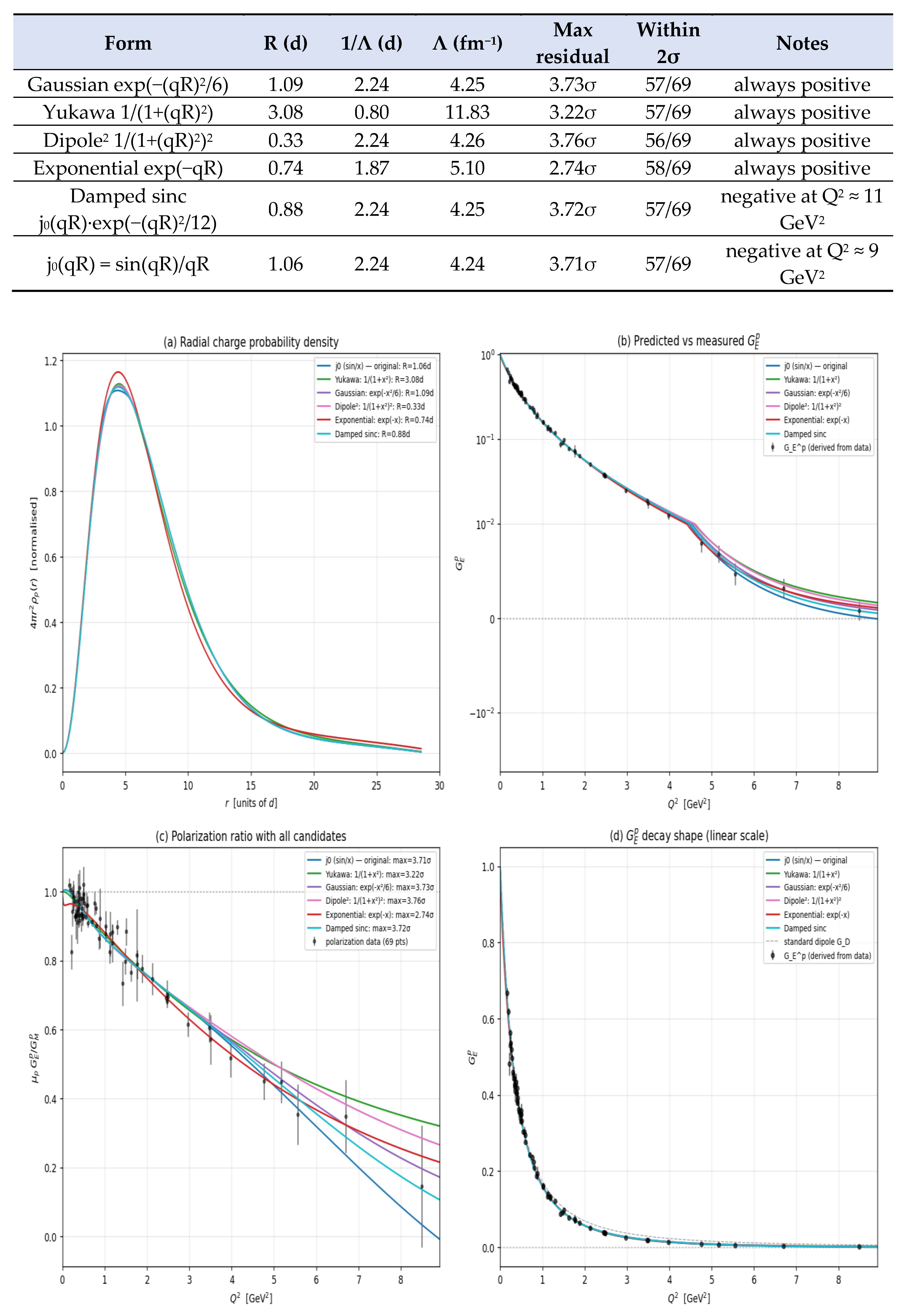
Five of the six candidates cluster around two natural V13 length scales: R ≈ 0.105 fm for the displacement and 1/Λ ≈ 0.21 fm for the dipole’s characteristic size. The exponential breaks out of this cluster with a smaller R and a slightly larger Λ; the Yukawa absorbs most of the dipole into its own falling form. The j0 and damped sinc, while fitting the data well within the measured Q2 range, both produce a small negative G_E^p at Q2 beyond current measurements — a behaviour that has not been observed and would require justification.
We adopt the Gaussian shift as the V13 description of the proton charge distribution:
with R ≈ 0.11 fm and 1/Λ ≈ 0.21 fm. R ≈ 0.11 fm is the off-centre shift parameter; 1/Λ ≈ 0.21 fm is the exponential decay rate of the real-space distribution. The radial probability 4πr2ρ(r) peaks near 0.42 fm and extends to 1.58 fm and beyond. The measured charge radius 0.84 fm is the RMS of this distribution — a statistical summary, not a hard boundary; roughly half the probability sits beyond it. Because elastic scattering resolves only the dense central region where two vortex cores cannot overlap, it measures this core size rather than the full extent of the vortex, which may reach considerably larger scales. The hyphons themselves remain intact lattice elements throughout.
G_E^p(Q2) = exp(−(qR)2/6) × 1 / (1 + Q2/Λ2)2
This is the same dipole/exponential form that describes the hydrogen 1s electron at atomic scale, scaled down by ≈ 2.5 × 10⁵.
5.3. The Neutron
The neutron is a proton with an additional bound electron and, pinned with it, the electron’s half-winding partner — a frozen antineutrino twist. The proton is essentially unchanged — same vortex pattern, same positron providing the +1e — and the electron is bound outside the core in its own probability cloud, giving net charge zero. The twist is the travelling helical wave of Section 5.5 brought to rest: free, its tilt direction rotates and averages out; bound, the rotation stops and the twist is pinned at a specific orientation, which is what gives the neutron’s internal structure its common axis. Like the positron in the proton, the electron has an exponential-like distribution at the lattice scale; the small but non-zero G_E^n signal arises from the slight asymmetry between these two near-mirror clouds.
The pinned twist is not optional decoration; the neutron’s spin requires it. A composite’s spin character follows a strict counting rule: orbital and geometric contributions are always integer, so half-integer total spin requires an odd number of half-winding constituents. A neutron built of proton and electron alone carries two halves — an integer — against the measured spin-½; carried into nuclei, the same count fails for the deuteron, helium-3, and nitrogen-14, the last being the historic 1930 argument that eliminated nuclear-electron models. With the pinned twist each bound electron brings two halves of its own (electron plus twist), and the count becomes the proton number mod 2: half-integer exactly for odd proton number — the measured rule, verified across neutron, deuteron, helium-3, tritium, helium-4, and nitrogen-14. The same bookkeeping forces beta decay’s antineutrino: three halves in, three out — its emission is winding-parity conservation, not a postulate. Measurement constrains which part of the neutrino flips and which is fixed: every neutrino observed has the same handedness, so the half-winding itself is pinned to the propagation, while the tilt phase is what rotates and averages to zero in flight. One honest flag: this rests on the same Z2 half-winding condition already named open in Section 5.1.3 — one condition, now underwriting three purchases.
β-decay is the release of this stored configuration. The neutron is heavier than its decay products by 0.782 MeV: the bound state is not deeply bound but metastable — the counter-chiral electron, excluded from the core (Section 5.2), sits in the shallow outer well holding that energy, and escape requires a lattice fluctuation to carry it over the confining barrier. The 880-second lifetime measures the height of that barrier, not the depth of a binding. At escape the pinned twist unpins and resumes travelling as the antineutrino, sharing the released energy; the proton’s charge is fully exposed and positive charge reappears. Inside a nucleus, neighbouring nucleons reshape the well and the exchange geometry, which is why bound neutrons are stable.
The neutron’s electric form factor follows directly from this picture. Treating both clouds with the same Gaussian-shifted-dipole form used for the proton in §5.2: G_E^n(Q2) = G_E^p(Q2) − G_E^e(Q2), with the proton’s parameters held fixed at their bare-proton values (R_p ≈ 0.115 fm, Λ_p = 4.25 fm−1), and only the electron parameters R_e and Λ_e fitted to the 38 measured G_E^n data points (Q2 = 0.01 to 3.41 GeV2).
The min-max fit gives R_e ≈ 0.21 fm and Λ_e = 3.97 fm−1 (1/Λ_e ≈ 0.25 fm). The model fits all 38 data points within 1.89σ on the worst residual, with χ2/N = 0.96 — comparable to the standard Galster (1.83σ, χ2/N = 0.90) and two-dipole (1.82σ, χ2/N = 0.90) parametrizations on the same data. The model gives ⟨r2⟩_n = −0.126 fm2, within 9% of the measured −0.116 fm2. No model in this comparison stands out as decisively better than the others — they all describe the data within similar precision, which is the same situation Galster has had for forty years. The V13 model is competitive with the standard fits while using a physical interpretation tied to the proton’s bare parameters.
Figure 5.
Neutron electric form factor in the V13 two-cloud picture. (a) Real-space charge probability density of the positron (fixed from §5.2), the electron (fitted), and the net neutron charge (positron − electron). (b) Predicted G_E^n compared to 38 measured data points (Riordan 2010, Madey 2003, Becker 1999, and others) for three parametrizations: Galster, two-dipole, and V13 with the proton parameters held fixed. (c) Residuals (data − model)/σ for each parametrization. (d) Decomposition of the V13 fit: G_E^n as the difference between the positron’s G_E (red) and the electron’s G_E (blue) — both falling smoothly from 1 at Q2 = 0. In panel (a) the radius axis is in units of d ≈ 0.105 fm.
Figure 5.
Neutron electric form factor in the V13 two-cloud picture. (a) Real-space charge probability density of the positron (fixed from §5.2), the electron (fitted), and the net neutron charge (positron − electron). (b) Predicted G_E^n compared to 38 measured data points (Riordan 2010, Madey 2003, Becker 1999, and others) for three parametrizations: Galster, two-dipole, and V13 with the proton parameters held fixed. (c) Residuals (data − model)/σ for each parametrization. (d) Decomposition of the V13 fit: G_E^n as the difference between the positron’s G_E (red) and the electron’s G_E (blue) — both falling smoothly from 1 at Q2 = 0. In panel (a) the radius axis is in units of d ≈ 0.105 fm.
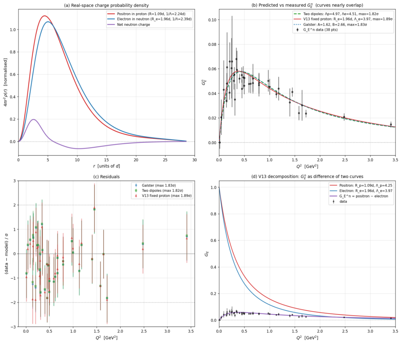
The result implies a definite physical picture: the electron in the neutron sits at roughly twice the off-center radius of the bare positron (R_e ≈ 0.206 fm versus R_p ≈ 0.115 fm) and is slightly broader than the positron (1/Λ_e ≈ 0.251 fm versus 1/Λ_p ≈ 0.236 fm, about 7% wider). The bound electron is more delocalized than the positron, consistent with its weaker binding. The Fourier transform of the difference produces the standard “neutron has positive core, negative shell” picture — a positive lobe at small r where the positron’s tighter distribution dominates, and a negative lobe further out where the electron’s wider distribution wins.
The magnetic moment follows the same two-cloud geometry. With circulation moments μ = evr/2 (Section 5.2), the positron at R_p contributes a small positive moment and the electron at its roughly doubled radius a larger negative one: the neutron’s negative magnetic moment — anomalous for a neutral particle in the naive picture — is automatic here, because the negative charge circulates on the wider orbit. The fitted radii give a net ≈ −0.4 μ_N against the measured −1.913 μ_N: sign and scale from geometry, the remaining factor open to the same knobs as the proton’s (vortex contribution, effective radii, circulation speed).
The same caveats apply as for any modern parametrization of G_E^n: the data are sparse (38 points across 3.4 GeV2 of Q2), some experiments have systematic disagreements, and the extracted electron parameters depend on the proton parameters being correctly fixed. The fit should not be over-interpreted as a definitive statement about the electron’s distribution inside the neutron; it is the closest the simple two-cloud picture comes to the measured form factor with parameters that match the bare proton.
5.4. Mesons and the Baryon-Meson Unification
The pion’s measured electromagnetic form factor F_π(Q2) is well-described by a monopole shape 1/(1 + Q2/Λ2), in contrast to the dipole-like shapes of the proton and neutron. The corresponding real-space charge density is a Yukawa-like exponential, ρ(r) ∝ exp(−Λr)/r, with a normal radial probability 4πr2ρ(r) that peaks at r ≈ 1/Λ and falls off exponentially. In this picture, the pion is simpler than a baryon: a single falling distribution rather than the offset, dipole-shaped distribution that the proton requires. The decay channel π+ → μ+ + ν fits this — the muon has a positron at its centre with no resolvable charge distribution, and the pion sits one step removed from that fully-static configuration.
The decay asymmetries of the pions read naturally in this picture. The π0 annihilates to two photons in 10−17 seconds: it is a configuration in which the opposite windings do reach contact — the endpoint of Section 5.1.1 completing — where the neutron’s geometry holds its pair apart for 880 seconds. The contrast between the two lifetimes is geometry, not a new interaction. The charged pion cannot annihilate completely — a net winding would remain — so it decays instead by reconfiguration, emitting a neutrino as winding parity requires (Section 5.3), and lives some 108 times longer. These readings are consistency observations, not derivations.
One correspondence is already fixed by the measurements: the preamble’s sphere-to-toroid transition maps onto the measured form-factor shapes. The proton’s dipole form factor corresponds to the ring form with an open eye; the pion’s monopole form factor to the simpler closed form with no eye — the measured 1/Q4 versus 1/Q2 fall-offs are the two shapes’ signatures. The detailed vortex topology distinguishing mesons from baryons beyond this correspondence, including how spin assignments emerge from different host geometries, is left for future work.
5.5. The Neutrino
The weak nuclear force does not exist as a separate force in this model. Beta decay and electron capture are the escape from and entry into the bound configuration of Section 5.3 — threshold physics of the neutron’s outer well, not a new interaction. What remains for this section is the particle those processes emit.
Earlier versions of this model identified the neutrino with the lattice’s longitudinal compression mode. That identification is withdrawn here, because measurement rules it out. In 1958 Goldhaber, Grodzins and Sunyar determined the neutrino’s helicity by measuring the polarization of a photon emitted opposite a neutrino in electron capture on europium-152: the spin is always locked antiparallel to the motion — every neutrino left-handed, every antineutrino right-handed. Fixed handedness is a rotational property, and a compression wave — rotationally symmetric about its direction of travel — has nothing that could carry it. The data decide against the earlier guess, and the correction is made openly.
The neutrino is identified instead as a travelling helical wave of the lattice’s orientational field — the same sector whose standing windings are the electron and positron (Section 5.1.3). The wave has two distinct aspects, and keeping them separate is what makes the measured properties consistent. The tilt phase rotates as the wave propagates: the local tilt direction, and with it any instantaneous charge-sector amplitude, sweeps around and averages to zero over every cycle — a flipping disturbance with zero mean, which is why the neutrino is neutral and why it is a wave rather than a standing defect: the two facts are one (Section 5.1.3). The handedness does not rotate: the sense of the helix is a half-integer winding of the same Z2 character conjectured for the electron’s spin, structurally locked to the propagation — this fixed sense is what helicity experiments measure, and ν and ν̄ are its two values. The same winding is why the neutrino barely interacts: scattering into light or compression would require converting a half-winding into an integer one, which no smooth lattice process can do. Transparency, neutrality, and spin-½ are three faces of one property. Pinned to a fixed orientation inside a neutron, this same wave is the frozen twist of Section 5.3; unpinned, it flies.
This object has a measured laboratory counterpart: the chiral phonon. Lattice waves that rotate while propagating, with handedness locked to the structure, are now directly observed — truly chiral phonons along the screw axis of α-HgS (Ishito et al., 2023), handedness-split phonon dispersion in quartz (Ueda et al., 2023), and, most relevantly, chiral acoustic phonons in α-quartz obeying pseudo-angular-momentum selection rules (Kim et al., 2026) — acoustic meaning they travel at the crystal’s sound speed, which in this lattice is c. On this identification the neutrino is the space lattice’s chiral acoustic phonon, upgraded from integer to half-integer winding. Everything except the half is observed physics. Two caveats keep the claim honest: measured chiral phonons carry integer winding, so the half remains this model’s addition, resting on the open Z2 condition; and the observed hosts are chiral crystals while this lattice is globally achiral — mitigated by the fact that both senses are needed anyway (ν and ν̄), so the medium must not prefer one.
That a half-winding can exist and survive in a real medium is itself measured: half-quantum vortices — a π orbital winding compensated by a π spin winding — have been observed and are robust in superfluid helium-3 (Autti et al., 2016). And helium-3-A hosts massless, chiral, luminal quasiparticles at its Fermi points (Volovik, 2003) — the established analogue class for a neutrino-like excitation of a condensed medium, with the caveat that its substrate is fermionic where this lattice’s is not.
The neutrino carries no rest mass: it is a wave, travelling at the medium’s wave speed by nature — which is why it moves at, or indistinguishably close to, c. Its speed is no longer conditioned on the longitudinal mode: as a wave of the orientational sector it rides the same channel as light, and the residual condition is only that the two circular senses propagate degenerately at c — the isotropy question of Section 3.1 in another form. What is detected as a small mass is not stored rest energy: lattice discreteness gives the helical mode a small dispersion correction at finite wavelength, so beta-decay neutrinos propagate slightly below c, and the launch recoil mimics inertia. The supernova SN1987A bound (|v/c − 1| < 10−9) and the KATRIN limit (m_ν < 0.45 eV) constrain the correction to be small but allow it to be non-zero — consistent with a discrete lattice.
The open conditions are listed explicitly. First, the Z2 half-winding: whether the four-sublattice orientational order supports it — one condition now underwriting the electron’s spin, the neutrino, and the neutron’s parity count (Section 5.1.3 and Section 5.3). Second, the flip bookkeeping: that the rotating tilt phase conserves angular momentum internally in flight is asserted, not derived. Third, whether the instantaneous charge amplitude averages to harmlessness at short probe scales is undetermined (Section 5.2). Fourth, flavour structure: the three flavours and their mass splittings are unassigned; three helical branches of the four-sublattice structure are a natural direction, not an identification. Fifth, the dispersion law has not been computed quantitatively against oscillation data. Of the identifications in this chapter, this is the one most likely to evolve: it is recorded as the best current understanding, expected to be revisited in future iterations of this work.
5.6. The Lorentz Factor and Rotational Speed
The relativistic energy formula E = γmc2, where γ = 1/√(1 − v2/c2), was derived by Hendrik Lorentz between 1892 and 1904 from the mechanics of objects moving through a stationary ether, before Einstein reinterpreted the same equations without reference to a medium.
In the vortex model, γ describes the energy cost of pushing a vortex through the ether lattice at translational speed v. As a vortex approaches c, the hyphons ahead have less and less time to move aside—the displacement signal travels at c, barely ahead of the vortex. At v = c the signal cannot propagate ahead at all, an infinite column of hyphons must be displaced simultaneously, and the energy diverges.
This is strictly a translational phenomenon. A spinning vortex does not push a column of lattice ahead—it rotates in place. Its neighbours feel the mismatch, but there is no infinite-column problem. Rotational speed has no theoretical ceiling. A vortex can spin at any rate. It cannot do so stably—the lattice bleeds energy from the over-spun vortex—but the instability is energetic, not kinematic. There is no rotational equivalent of the γ divergence.
The column picture can be made quantitative, and it yields a formula. The relativistic relation E2 = (m0c2)2 + (pc)2 can be rewritten exactly as γ = √(1 + L/d), where L = d·(p/m0c)2. Read mechanically: the inertia of a moving pattern is set by the length L of the hyphon column it must carry, measured in lattice spacings, and that column grows as the square of the momentum. On a straight path L is free to grow without limit, and the divergence of γ at v = c is the infinite-column statement above in algebraic form.
Circular motion bounds the column geometrically: an orbit of radius r cannot coherently recruit more than a length ~κr of forward column, with κ an order-one geometric factor. Writing 1/L_eff = 1/(dβ2γ2) + 1/(κr), the effective inertia m_eff = m0√(1 + L_eff/d) recovers the standard γ exactly as r → ∞, but in tight orbits it turns a knee near m0√(1 + κr/a), where a is the spacing of the lattice’s own elements. Past that knee the simplified form levels off, and that plateau is where it fails: the dragged column shears against the medium outside it and entrains that in turn, layer by layer. What the speed of light limits is the slip between neighbouring layers, not the speed of the defect against the distant lattice — so a faster orbit is accommodated by entraining more layers rather than by refusing to go faster, and the inertia keeps rising without bound instead of saturating. The consequence for rotation is unchanged and now has a mechanism behind it: circulation faster than c is permitted at finite energy, costing more than circulation at c rather than being forbidden, because the c-limit constrains transport, not rotation. A quantitative, speed-dependent entrainment law is left to future work (Figure 6). Two consequences follow. At r comparable to the lattice spacing — the bound positron’s orbit in the proton core (Section 5.2) — the inertia caps near √2 m0, so core circulation above c costs little. And in any laboratory ring the electron should be fractionally lighter than γm0, by Δγ/γ ≈ (β4γ2/2κ)(d/r): about 10−10 at LEP’s 3 km bending radius — five orders below the 2×10⁻⁵ precision of resonant-depolarization calibration, consistent with every existing measurement while remaining, in principle, a falsifiable departure from special relativity. The rewriting itself is exact; what this model adds is the column interpretation and the geometric cutoff, whose form and constant κ are not derived here. Whether the diverging part of a fast defect’s co-moving field in fact resides in the forward column rather than in a contracting core — as it does for one-dimensional lattice kinks — is a computable property of this lattice, and it decides whether the cutoff operates.
5.7. The Gyroscopic Lattice: Laboratory Realisation and the Reciprocity Constraint
A second laboratory system supports the picture of space as a lattice of spinning elements. Nash et al. (2015) built a “gyroscopic metamaterial”—coupled spinning gyroscopes arranged on a lattice—and showed experimentally that it has a genuine vibrational band structure with a sonic gap, behaving as a rigid, dispersive medium of a kind no gas can imitate. This is a direct realisation of the central assumption of the present model: that a lattice whose elements carry intrinsic spin is a real mechanical medium with its own wave speed and dispersion relation, not merely a fluid.
The same work raises the sharpest objection to a spinning-element vacuum, and points to its answer. Nash et al. found that a lattice of gyroscopes all spinning in the same sense breaks time-reversal symmetry and carries waves preferentially in one direction—its edge modes are chiral and non-reciprocal. They further showed that this symmetry breaking is set by the lattice bond-angle distribution together with the common spin direction. A vacuum built this way would be optically handed, which experiment excludes to very high precision.
The hyphon lattice escapes this because its spins are not aligned. The four FCC sublattices spin along the four tetrahedral axes and pair into two antiparallel groups (Section 2.1); neighbouring hyphons rotate oppositely, so the net angular momentum and the macroscopic time-reversal bias cancel, while the local torsional stiffness that carries light survives. The gyroscopic metamaterial is therefore both the closest engineered analogue of the model and the experiment that fixes a necessary property of the spin arrangement: the vacuum can be gyroscopic at the element scale only if it is non-chiral in bulk, which the opposite-spin sublattice structure guarantees. This constraint closes a loop with Section 5.2 and Section 5.5. The measured physics that would make an aligned lattice handed — spin sense steering waves preferentially — is the same physics class as the chirality-selective force of Section 5.2: near a single vortex the spin sense does discriminate, binding the co-chiral defect and excluding the counter-chiral one; the sublattice cancellation removes the bias only in the bulk average, not locally. And the achiral bulk is exactly what the neutrino picture requires: with no preferred handedness, the two helical senses of Section 5.5 propagate as a degenerate pair — ν and ν̄ on equal footing — which is the residual speed condition of that section restated. One measured system, three duties: analogue, constraint, and consistency check.
6. Nuclear Structure
Nucleons are vortex configurations of comparable size in the hyphon lattice. Protons carry charge (+1e); neutrons are the same vortex with a bound electron cancelling the charge, plus its pinned antineutrino twist (Section 5.3). Inside nuclei, the cores order themselves in rock salt (NaCl-type) arrangement: protons and neutrons on alternating sublattices. The entire rock salt structure inherits the 54.74° tilt from the hyphon lattice — all nucleon spin axes point along body diagonals, and the natural packing planes are (111) hexagonal layers. The arrangement of nucleons on an FCC lattice with alternating proton-neutron ordering has a substantial history. The FCC symmetry of nuclear quantum states was first identified by Wigner (1937). Cook (1994, 2010) developed this into a comprehensive lattice model, showing that the FCC geometry reproduces the quantum numbers of the independent-particle model, the liquid drop properties, and alpha cluster substructures within a single framework — and computed binding energies for over a thousand nuclei and charge radii for 341 isotopes. Garai (2003) showed that the proton positions in FCC double tetrahedra correlate with all nuclear quantum numbers. The present work arrives at the same nuclear ordering from a different starting point: the rock salt alternation emerges from Coulomb energetics of charged and screened vortex spheres, and the nuclear lattice is embedded within a more fundamental hyphon FCC lattice with the nucleon vortices themselves borderless and overlapping, their charge distributions centred 1.85 fm apart.
A note fixes the picture used throughout this chapter: a nucleon vortex has no outer border. The 0.84 fm charge radius is a scale of the charge distribution, not a wall; the flow field extends beyond it with no defined edge — plausibly, at low amplitude, out to atomic scale — and neighbouring nucleons’ flow fields interpenetrate freely. The core — the vortex’s eye — is where the bound positron sits. The nuclear force is the interaction of these overlapping flows, not a contact between surfaces; and the neutrons’ role in a nucleus is to supply the nuclear electrons whose orbits screen the repulsion between the positrons in the proton cores (Section 6.2). The borderless picture is applied consistently in what follows, but its consequences — how far the flow fields reach, and what sets the strength profile of the overlap interaction — are only partly worked out; like Section 5.5, this chapter is expected to be revisited in future iterations of this work.
6.1. Rock Salt Ordering and Nuclear Density
The alternating arrangement arises from Coulomb energetics. All nucleon cores are identical proton-core vortices carrying charge +1e. In an N = Z nucleus, Z delocalized electrons flow through the lattice channels between them (Section 6.2). At any instant, a core with an electron nearby appears electrically neutral — a neutron — while a bare core appears as a proton. This proton–neutron distinction is a snapshot of the electron positions, not a permanent property of the cores. In this snapshot picture, the lowest-energy arrangement places protons and neutrons on alternating sites: each proton has 6 neutron nearest neighbours and vice versa, the standard rock salt geometry.
Figure 7.
He-4 (alpha particle) cross-section along the hexagonal plane. Rock salt ordering places proton vortex cores (red gradient) and neutron vortex cores (blue gradient, vortex + bound electron) on alternating corners. Dotted circles show the proton charge radius (≈ 0.84 fm). Two delocalized electrons (yellow ‘e’) flow between cores. The FCC hyphon lattice (small colour-coded spheres) fills all space outside the nucleon vortex regions. Centre-to-centre spacing 1.85 fm. Three states of the same medium are visible: nucleon vortex regions, the surrounding charge field (overlapping charge distributions), and free lattice (undisturbed FCC pattern). Axes and labels in the figure are in units of d ≈ 0.105 fm.
Figure 7.
He-4 (alpha particle) cross-section along the hexagonal plane. Rock salt ordering places proton vortex cores (red gradient) and neutron vortex cores (blue gradient, vortex + bound electron) on alternating corners. Dotted circles show the proton charge radius (≈ 0.84 fm). Two delocalized electrons (yellow ‘e’) flow between cores. The FCC hyphon lattice (small colour-coded spheres) fills all space outside the nucleon vortex regions. Centre-to-centre spacing 1.85 fm. Three states of the same medium are visible: nucleon vortex regions, the surrounding charge field (overlapping charge distributions), and free lattice (undisturbed FCC pattern). Axes and labels in the figure are in units of d ≈ 0.105 fm.
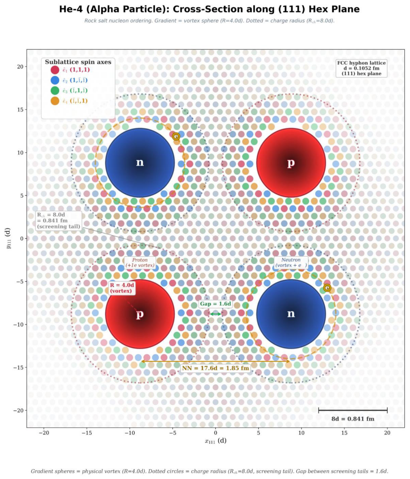
This ordering also follows from the sublattice geometry of the hyphon lattice itself. In the FCC structure, nearest neighbours always belong to different spin sublattices, while second-nearest neighbours belong to the same sublattice. The four tetrahedral spin orientations pair naturally into two antiparallel groups — {S0,S1} vs {S2,S3} — whose net spins oppose at 180°. This two-group alternation on an FCC lattice is rock salt ordering, which Canuto & Chitre (1974) showed is the antiferromagnetic ground state. The rock salt structure is therefore not assumed — it is the lowest-energy configuration that the hyphon lattice geometry requires.
In heavy nuclei at saturation density (0.16 nucleons/fm3), rock salt ordering gives a nearest-neighbour distance of 1.85 fm. With charge-distribution radius 0.84 fm, the characteristic extents of neighbouring charge clouds stop about 0.17 fm short of one another — the distributions remain distinct — while the flow fields, having no borders, overlap throughout. Nucleons interact through this flow overlap and through the shared lattice, not by surface contact.
He-4 (4 proton cores + 2 delocalized electrons) is the minimal rock salt unit — a square with cores of one orientation pair on opposite corners. Being the lightest nucleus, He-4 is less dense than bulk nuclear matter, with a nearest-neighbour distance of approximately 2.05 fm. Its charge radius (1.676 fm) is within 0.5% of twice the proton charge radius (0.841 fm; Pohl et al., 2010). The discrete square geometry gives R_ch = √(d2_nn/2 + R2_p) = 1.676 fm — a 99.9% match to experiment. A tetrahedral arrangement (as in Cook’s FCC model without sublattice ordering) gives approximately 1.50 fm — inconsistent with the measured value. The charge radius formula R_ch = √(3/5 × (r0(2Z)^{1/3})2 + R2_p), applied across 285 isotopes (Z = 1–83), gives R2 = 0.988 — comparable to Cook’s empirical result (R2 = 0.979), confirming uniform proton-core density in the N = Z core.
The rock salt picture is a bulk approximation that works well for nuclei above carbon (A ≥ 12, charge radius errors below 3%) but breaks down for light nuclei — errors exceed 20% for A ≤ 4, where a uniform-density sphere is meaningless for just a few nucleon cores. For these systems, the charge radii and binding energies depend on the specific geometry of proton core positions and the delocalized electron orbits described in the next section, requiring a detailed treatment of Coulomb screening and the strong force rather than a statistical bulk formula.
6.2. Electron Delocalization Inside Nuclei
In a free neutron, the electron is held in the shallow outer well of Section 5.3, storing 0.782 MeV of releasable energy — barely held, as demonstrated by the neutron’s 10-minute decay half-life. When a second proton core approaches to nuclear distance, its Coulomb pull on the electron competes with the parent proton’s hold. The electron, already on the verge of escape, detaches from one core and is captured by the other. The resulting orbit is a shared path between the two cores — most likely a figure-8 with the crossing point between them, though an elongated racetrack (two half-orbits connected by near-straight segments along the cores’ edges) is also geometrically possible depending on the electron speed and core separation. In either topology, the electron visits both proton cores in each cycle, screening their mutual Coulomb repulsion. The idea that neutron electrons delocalize between proton cores inside nuclei was independently proposed by Cziráki (2023), who described the nucleus as protons held together by collectivized electrons in a covalent-like bond. The present work arrives at the same conclusion from a different starting point — the hyphon lattice mechanics — and develops the orbital geometry, screening calculations, and geometric frustration picture in detail.
Once detached, the electron flies to the neighbouring proton core, enters the strain well near its core, completes a half-orbit on the far side (where both protons pull inward, strengthening the anchor), then reaches the near side and detaches again — returning to the first core. At each crossing, the electron detaches from one core (beta decay) and is captured by the other (inverse beta decay), its pinned antineutrino twist (Section 5.3) transfers with it, so nothing is emitted and no energy is lost per crossing. Inside the nucleus the exchange is a closed loop: every detachment is immediately followed by capture at the next core, the twist riding along throughout. The “weak force” is what this continuous exchange looks like from outside when the loop breaks: in a free neutron, the electron detaches with no nearby core to catch it, the twist unpins, and both the electron (beta particle) and the freed antineutrino escape to infinity.
Figure 8.
Deuterium: figure-8 electron exchange orbit. One electron (yellow) traces a shared path between two proton cores (red, core separation 3.75 fm, r_e = 0.907 fm) whose spin axes are tilted at 109.47° (the tetrahedral angle between their respective sublattice directions). At each crossing point, the electron detaches from one core (β− decay) and is captured by the other (inverse β−), its pinned antineutrino twist transferring with it — nothing is emitted in the closed loop (Section 5.3).
Figure 8.
Deuterium: figure-8 electron exchange orbit. One electron (yellow) traces a shared path between two proton cores (red, core separation 3.75 fm, r_e = 0.907 fm) whose spin axes are tilted at 109.47° (the tetrahedral angle between their respective sublattice directions). At each crossing point, the electron detaches from one core (β− decay) and is captured by the other (inverse β−), its pinned antineutrino twist transferring with it — nothing is emitted in the closed loop (Section 5.3).
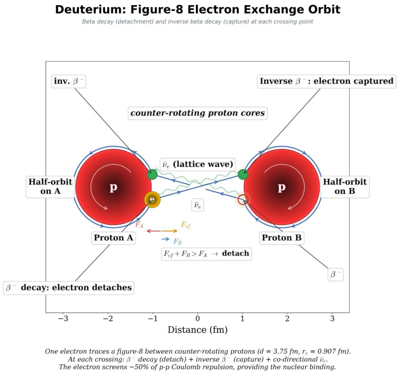
The figure-8 electron screens approximately 50% of the proton–proton Coulomb repulsion, computed by time-averaging the net electromagnetic force over 720 electron positions around the full orbit. One electron cannot neutralise two protons — when the electron is on the far side of its current core, it pulls that core away from the other, adding to the repulsion. The near-side phases are attractive (approximately −1.0 MeV/fm), the far-side phases repulsive (+1.2 to +1.6 MeV/fm depending on core separation), and the time average is roughly 50% screening at all distances tested (2.0 to 5.0 fm).
For three proton cores (tritium, He-3), the topology changes. He-3 has one electron for three cores. One proposed orbit is a trefoil — the electron visiting all three cores in sequence, screening each edge for one-third of the period. Other topologies, such as a figure-8 between two of the three cores, would screen those two more effectively but the third less so. Regardless of the exact topology, He-3 is stable: it has the minimum possible electron count (one) for three cores, and removing it would leave three bare protons — no nucleus. Tritium has two electrons for three edges: two edges screened, one frustrated. The geometric frustration drives tritium’s beta decay (half-life 12.3 years) — the frustrated electron eventually escapes, leaving He-3. The binding energy difference between tritium and He-3 (0.764 MeV) is a direct measurement of one electron’s screening contribution.
Figure 9.
He-3: proposed trefoil electron orbit. One electron (yellow) shared among three proton cores (P1, P2, P3). In the proposed topology, the electron visits all three cores in sequence, performing a half-orbit on each before detaching to the next (β−/inverse β− at each crossing), screening each edge for one-third of the orbital period. The He-3 triangle is 15% larger than tritium’s (less screening → more Coulomb repulsion).
Figure 9.
He-3: proposed trefoil electron orbit. One electron (yellow) shared among three proton cores (P1, P2, P3). In the proposed topology, the electron visits all three cores in sequence, performing a half-orbit on each before detaching to the next (β−/inverse β− at each crossing), screening each edge for one-third of the orbital period. The He-3 triangle is 15% larger than tritium’s (less screening → more Coulomb repulsion).
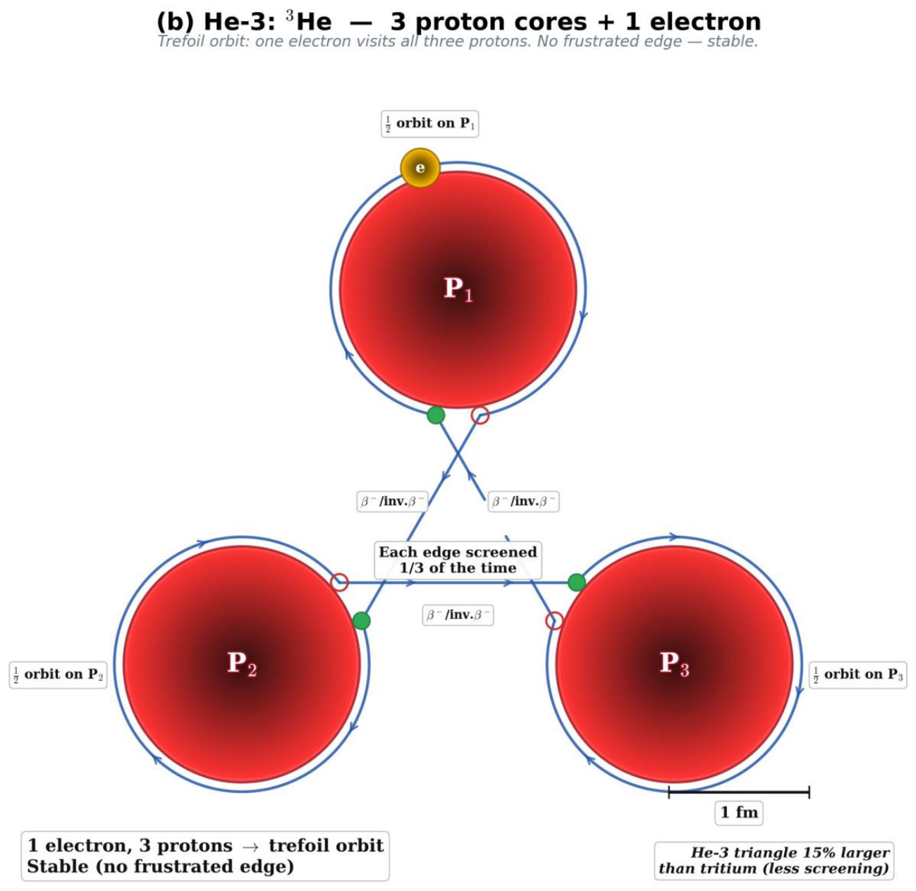
He-4, with four proton cores on a rock salt square and two electrons, achieves the most symmetric configuration: each electron traces a figure-8 along one diagonal, screening both diagonals simultaneously with the electrons maximally separated. No edge is frustrated. Every core is equivalent. This perfect coverage, combined with the strong-force binding from four nearest-neighbour flow overlaps, produces a binding energy per nucleon of 7.07 MeV — higher than any nucleus below carbon-12, the famous alpha-particle peak.
In nuclei larger than He-4, the electron does not simply turn around at each core. With multiple proton cores packed in rock salt ordering, the next core along the same [111] channel pulls the electron forward. The electron threads through the nuclear interior on an S-shaped path: half-orbit on one core’s surface, detach, cross the ~0.35 fm between neighbouring charge clouds, capture at the next core, half-orbit on the opposite side, detach again — continuing until it reaches the nuclear surface. At the surface, with no forward core, the electron completes a full orbit before heading back along a different [111] channel. Surface nucleons that retain a complete electron orbit are what we observe as neutrons; interior cores, constantly flickering between bare and screened as electrons pass through, have no fixed proton or neutron identity. This is the physical origin of isospin symmetry — the experimental observation that protons and neutrons are nearly interchangeable inside nuclei.
Figure 10.
Carbon-12: S-path through a [111] channel. One electron (yellow) threads through the nuclear interior, performing alternating half-orbits on successive proton cores (red). At each surface neutron (blue), the electron completes a full orbit before reversing along a different channel.
Figure 10.
Carbon-12: S-path through a [111] channel. One electron (yellow) threads through the nuclear interior, performing alternating half-orbits on successive proton cores (red). At each surface neutron (blue), the electron completes a full orbit before reversing along a different channel.
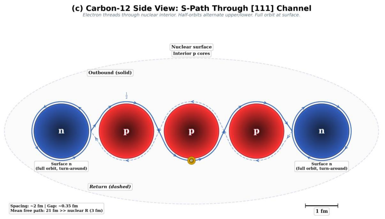
For any N = Z atom, the electrons split exactly in half: Z electrons orbit inside the nucleus between proton cores at ~2 fm spacing, providing ~MeV-scale screening, and Z electrons orbit outside the nucleus around it at ~50,000 fm spacing, forming ~eV-scale chemical bonds. Both sets do the same job — thread between positive centres and screen their mutual repulsion — at different distance scales. The deuteron, with its full electron complement, is the nuclear analogue of H2: two proton cores sharing two electrons, one on a nuclear-scale figure-8 orbit (~2 fm, ~MeV binding) and one on an atomic-scale orbit (~50,000 fm, ~eV binding). The nuclear subsystem alone — two proton cores plus one shared electron — maps to H2+. The analogy is not perfect: the nuclear bond additionally has the strong force — here, the overlapping-flow interaction — which dominates the binding energy. At atomic distances, no strong force operates and the bond is purely electromagnetic.
6.3. Heavy Nuclei and Neutron Excess
In light nuclei (A ≤ 40), rock salt ordering gives a 1:1 proton-neutron ratio. In heavy nuclei, cumulative Coulomb repulsion between protons raises the energy of the interior. Extra neutrons attach to the nuclear surface as a neutral skin, reducing the Coulomb stress without disrupting the 1:1 rock salt core. Even for lead-208 (44 excess neutrons), the extra neutrons occupy only ~18% of the available core surface area — surface-only accommodation is geometrically sufficient through the entire periodic table. Ca-40 and Ca-48 have the same charge radius (3.478 vs 3.477 fm) despite 8 extra neutrons — confirming that the proton-neutron core stays the same size and the extra neutrons pack outside it.
7. Electromagnetism
7.1. Charge
Charge arises from the lattice’s orientational sector. The electron is a wound defect — a localized winding of the hyphon spin axes (Section 5.1) — and the proton’s +1e is the same object of opposite winding, bound co-chirally in the vortex core (Section 5.2). What we measure as electromagnetic interaction is the interaction of the overlapping tilt fields: the elastic energy goes as the square of the total tilt, so same-sense windings reinforce and are pushed apart, opposite-sense windings cancel and are pulled together — like repels, opposite attracts, from one cross-term (Section 5.1.1). The class behaviour is established in real systems: kinks in the Frenkel–Kontorova model interact with exactly this sign structure (Braun & Kivshar, 1998); orientational point defects with emergent Coulomb interaction are observed directly in nematic liquid crystals and in superfluid helium-3 (Volovik, 2003); and an elastic continuum that resists shear but not compression has equations of motion isomorphic to Maxwell’s, with charge as a defect producing a 1/r field (the rotational-ether result of MacCullagh, made rigorous by Dmitriyev, 2004). This also distinguishes charge from gravity: the pressure deficit of Section 4 is single-signed and can only attract, while winding is genuinely two-signed. The 1/r range follows from harmonic relaxation; the open end, stated in Section 5.1.1, is the strength — with the deeper question of exact isotropy and full Lorentz invariance shared with emergent gauge fields in superfluid helium-3.
The positron in a proton produces the same unit of charge as a free positron would — it is the same wound defect, carrying the same winding. What differs is the measured spatial distribution: in a proton, the positron interacts with the surrounding vortex body, which shapes its distortion pattern and produces the observed ~fm-scale charge distribution. In the free case, the distortion extends directly into the undisturbed lattice and the defect appears point-like (electron-positron scattering experiments constrain any internal structure below 10−18 m). Details of the proton’s charge distribution are addressed in Section 5.2.
The electron and positron are created as a pair — equal and opposite lattice distortions that together leave the lattice unchanged. Their charges are equal by construction. The proton carries charge +1e because a positron — the same wound defect mirrored — is bound co-chirally in its core (Section 5.2), its charge equal to the free positron’s by construction (measured to one part in 1021). There is no half-unit of mismatch — one winding, one unit of charge. This is why fractional charges do not exist as free particles.
Each charged particle creates a distortion pattern in the surrounding lattice that radiates outward as a 1/r field. When two particles create the same type of distortion, the patterns reinforce between them — the lattice stores more strain energy in the overlap, and the system lowers its energy by moving them apart. This is repulsion. When two particles create opposite distortions, the patterns cancel between them — the lattice relaxes in the gap, and the surrounding pressure pushes them together. This is attraction. No force carrier is needed — the lattice itself, seeking its minimum energy configuration, produces the force.
Charge does not appear or disappear instantaneously in its surrounding field. When an electron-positron pair forms (for example from a high-energy photon pair producing e− + e+), the hyphons around each newly created winding must physically rearrange to accommodate the distortion. This rearrangement propagates outward at c: inside an expanding sphere of radius ct around the creation event, the new field pattern is established; outside it, the lattice has not yet received the news of the new charges. The reverse happens when an electron and positron meet and annihilate: the distortion around each winding must un-rearrange, and this inverse wavefront also propagates outward at c, converting the stored strain into electromagnetic radiation (the annihilation photons carry away the energy previously bound into the pair’s windings and the rest mass). In both cases, the lattice response is a one-time longitudinal rearrangement radially around the event, consistent with the geometry-dependent mode selection described in Section 3.1: radial sources excite longitudinal modes.
7.2. Magnetism
7.2.1. Magnetism as Moving Charge Distortion
A stationary charged particle creates a spherically symmetric distortion pattern in the lattice — the electric field (Section 7.1). When the particle moves, this distortion pattern moves with it. But the lattice is not instantaneous: the distortion at the old position fades as the lattice relaxes, while the distortion at the new position builds up as the lattice deforms. This creates an asymmetry — the distortion pattern of a moving charge is no longer purely radial. It acquires a circular component that wraps around the direction of motion. This circular component is the magnetic field. Magnetism is not a separate force — it is the lattice’s response to charge distortion in transit. In standard physics this is well known: the magnetic field is the relativistic correction to the electric field for moving charges. In the lattice model the same result has a mechanical origin — the lattice cannot deform and relax instantaneously, so a moving source of distortion leaves a swirling wake.
7.2.2. Current-Carrying Wire
In a straight current-carrying wire, many electrons propagate through the lattice in the same direction. Each moving distortion pattern creates a circular component that propagates outward (Section 7.2.1). The patterns from all electrons along the wire add coherently — they all swirl the same way around the wire. The combined circular distortion falls as 1/r (spreading over a circumference 2πr), producing the magnetic field measured around any current-carrying conductor.
7.2.3. Magnetic Dipole
A single orbiting electron — or any current loop — creates a circular distortion from each segment of its path. From far away, opposite sides of the loop produce swirls that partially cancel. What survives is weaker and falls as 1/r3 — the magnetic dipole field. The magnetic moment of an atom is set by its electron’s orbital plane and speed.
7.2.4. Permanent Magnets and Materials
A permanent magnet is a collection of atoms whose electron orbital planes are aligned. Their individual circular distortion patterns add coherently, producing a macroscopic magnetic field. In most materials the orbital planes are random and cancel — no net field. In ferromagnetic materials, the lattice coupling between neighbouring atoms’ electron orbits allows an external magnetic field to align them. Soft magnetic materials reorient easily; hard magnetic materials resist reorientation but retain alignment once achieved. Above the Curie temperature, thermal vibration overwhelms the alignment and magnetism is lost.
7.2.5. Electromagnetic Induction
When a magnetic field changes — because a magnet moves or a current varies — the circular distortion pattern shifts through the lattice. Any electron in the path of this shifting pattern gets pushed by the changing lattice strain, producing a current. This is Faraday’s law: changing magnetic flux induces an electromotive force. In the lattice model it is purely mechanical — a moving strain pattern pushes charges, just as a water wave pushes a floating object.
7.3. Lightning and Electrical Discharge
Lightning and electrical discharge occur when the charge distortion in the lattice exceeds a critical threshold. In normal conduction, electron excitations hop between hyphons one at a time, each hop requiring energy to overcome the lattice coupling barrier. The distortion field from a charge imbalance strains the lattice along the field direction, lowering this barrier. At sufficient field strength, the first electrons begin hopping through where the field is locally strongest. Their motion creates flow-like distortion along the path, which drops the local lattice pressure by the same Bernoulli mechanism that produces gravity (Section 4). Lower pressure means a slightly stretched lattice — weaker coupling between elements — and easier hopping. Each additional electron deepens the low-pressure channel, making the next hop easier still. Meanwhile, the circular magnetic distortion around the channel (Section 7.2.1) raises pressure outside, confining the low-pressure tube to a narrow path. The result is a self-reinforcing, self-focusing avalanche: a temporary vortex tube in the lattice with low pressure inside (easy conduction) and high pressure outside (barrier). The stepped leader observed in lightning is this avalanche propagating in stages — advancing where the field is strong, pausing where it weakens, building up distortion, then jumping again. Once the channel connects the charge reservoirs, the full imbalance discharges through the low-pressure path in microseconds (the return stroke). The rapidly changing current produces intense electromagnetic radiation because the hop pulses no longer cancel as they do in steady current. Once the charge imbalance equalises, the flow stops, pressure normalises, and the lattice relaxes to its ground state.
8. Chemistry
The chemical bond is the same electron-sharing mechanism operating at atomic distances without the strong force. Two atomic nuclei separated by ~1 Å share one or more electrons that thread through the hyphon lattice between them, screening their mutual Coulomb repulsion — precisely as nuclear electrons screen proton cores at ~2 fm.
9. Acknowledgements and Invitation to Collaboration
This document presents the framework at varying stages of development. Higher confidence: the lattice as the medium of space, light as transverse lattice waves, gravity as a vortex pressure gradient, and time dilation as a local lattice property — these form a coherent core whose internal consistency and correspondence with established physics is strong. Also higher confidence within the particle section: the identification of electrons and positrons as wound defects of the lattice’s orientational sector, the neutron as a proton with a bound electron and its pinned antineutrino twist, and the charge-distribution picture from probability clouds. The neutrino identification (Section 5.5) is recorded as best current understanding, expected to evolve. Lower confidence: the detailed proton vortex geometry, its full spatial extent, and possible atom-scale structure — these are included to show where the framework points, but at lower confidence than the core material. Many further details have been omitted not because they do not exist, but because they require further development before being defensible at the same level.
The author is not an expert in all the fields this theory touches—fluid dynamics, nuclear physics, general relativity, quantum mechanics, and cosmology each have deep bodies of knowledge that deserve more rigorous treatment than one individual can provide. Significant work remains: matching existing experimental formulas to this model, deriving the vortex pressure profiles from first principles, and creating fluid dynamics models or CFD simulations to produce a quantitative picture.
Collaboration with physicists, mathematicians, and computational scientists who find these ideas worth exploring would be greatly welcomed—whether in formalising the mathematics, identifying experimental tests, uncovering errors, or developing the many details that this framework leaves open.
References
- Abbott, B. P. et al. [LIGO Scientific Collaboration and Virgo Collaboration] (2016). Observation of gravitational waves from a binary black hole merger. Physical Review Letters, 116(6), 061102. [CrossRef]
- Abbott, B. P. et al. [LIGO Scientific Collaboration and Virgo Collaboration] (2017). GW170817: Observation of gravitational waves from a binary neutron star inspiral. Physical Review Letters, 119(16), 161101. [CrossRef]
- Andreev, A. F., & Lifshitz, I. M. (1969). Quantum theory of defects in crystals. Soviet Physics JETP, 29(6), 1107–1113.
- Autti, S. et al. (2016). Observation of half-quantum vortices in topological superfluid 3He. Physical Review Letters, 117(25), 255301. ttps://doi.org/10.1103/physrevlett.117.255301.
- Bell, J. S. (1964). On the Einstein Podolsky Rosen paradox. Physics Physique Fizika, 1(3), 195–200.
- Bonometti, T., & Magnaudet, J. (2006). Transition from spherical cap to toroidal bubbles. Physics of Fluids, 18(5), 052102. [CrossRef]
- Bramwell, S. T., Giblin, S. R., Calder, S., Aldus, R., Prabhakaran, D., & Fennell, T. (2009). Measurement of the charge and current of magnetic monopoles in spin ice. Nature, 461(7266), 956–959. [CrossRef]
- Braun, O. M., & Kivshar, Y. S. (1998). Nonlinear dynamics of the Frenkel–Kontorova model. Physics Reports, 306(1–2), 1–108. [CrossRef]
- Canuto, V., & Chitre, S. M. (1974). Crystallization of dense neutron matter. Physical Review D, 9(6), 1587–1613. [CrossRef]
- Castelnovo, C., Moessner, R., & Sondhi, S. L. (2008). Magnetic monopoles in spin ice. Nature, 451(7174), 42–45. [CrossRef]
- Clauser, J. F., Horne, M. A., Shimony, A., & Holt, R. A. (1969). Proposed experiment to test local hidden-variable theories. Physical Review Letters, 23(15), 880–884. [CrossRef]
- Cook, N. D. (1994). Nuclear binding energies in lattice models. Journal of Physics G, 20, 1907–1917. [CrossRef]
- Cook, N. D. (2010). Models of the Atomic Nucleus: Unification Through a Lattice of Nucleons (2nd ed.). Springer.
- Crawford, C. B. et al. (2007). Measurement of the proton’s electric to magnetic form factor ratio from 1H(e, e′p). Physical Review Letters, 98(5), 052301. [CrossRef]
- Cziráki, Á. (2023). Stability of nuclei based on the new proton and neutron model. Natural Science, 15(12), 289–299.
- Dirac, P. A. M. (1951). Is there an aether? Nature, 168, 906–907.
- Dmitriyev, V. P. (2004). Elasticity and electromagnetism. Meccanica, 39(6), 511–520. (Maxwell’s equations as an incompressible shear-elastic continuum; electric charge as a lattice defect with a 1/r field.).
- Ekholdt, R. (2009). A soliton model of the electron with an internal nonlinearity cancelling the de Broglie–Bohm quantum potential. arXiv:0906.0598.
- Feynman, R. P. (1955). Application of quantum mechanics to liquid helium. Progress in Low Temperature Physics, 1, 17–53.
- Fizeau, H. (1851). Sur les hypothèses relatives à l’éther lumineux. Comptes Rendus de l’Académie des Sciences, 33, 349–355.
- Garai, J. (2003). The double tetrahedron structure of the nucleus. arXiv:nucl-th/0309035.
- Galster, S., Klein, H., Moritz, J., Schmidt, K. H., Wegener, D., & Bleckwenn, J. (1971). Elastic electron-deuteron scattering and the electric neutron form factor at four-momentum transfers 5 fm−2 <q2 <14 fm−2. Nuclear Physics B, 32(1), 221–237. [CrossRef]
- Girifalco, L. A., & Weizer, V. G. (1959). Application of the Morse Potential Function to Cubic Metals. Physical Review, 114(3), 687–690. [CrossRef]
- Goldhaber, M., Grodzins, L., & Sunyar, A. W. (1958). Helicity of neutrinos. Physical Review, 109(3), 1015–1017. [CrossRef]
- Hall, H. E., & Vinen, W. F. (1956). The rotation of liquid helium II: The theory of mutual friction in uniformly rotating helium II. Proceedings of the Royal Society A, 238(1213), 215–234. [CrossRef]
- Hill, M. J. M. (1894). On a spherical vortex. Philosophical Transactions of the Royal Society of London A, 185, 213–245. [CrossRef]
- Hivet, R. et al. (2012). Half-solitons in a polariton quantum fluid behave like magnetic monopoles. Nature Physics, 8(10), 724–728. [CrossRef]
- Hoek, M. (1868). Determination de la vitesse avec laquelle est entraîné un rayon lumineux. Archives Néerlandaises des Sciences Exactes et Naturelles, 3, 180–185.
- Ishito, K. et al. (2023). Truly chiral phonons in α-HgS. Nature Physics, 19(1), 35–39. [CrossRef]
- Jones, M. K. et al. [Jefferson Lab Hall A Collaboration] (2000). G_Ep/G_Mp ratio by polarization transfer in polarized ep scattering. Physical Review Letters, 84(7), 1398–1402.
- Kim, C., Hwang, I.-K., Moon, K.-W., An, K., Lee, K.-J., Ko, J.-H., Park, B.-G., Choi, K.-Y., & Hwang, C. (2026). Chiral acoustic phonon and conservation of pseudoangular momentum in α-quartz. Advanced Materials. [CrossRef]
- Landau, L. D. (1933). Über die Bewegung der Elektronen im Kristallgitter. Physikalische Zeitschrift der Sowjetunion, 3, 664–665.
- Landau, L. D. (1941). Theory of the superfluidity of helium II. Physical Review, 60(4), 356–358. [CrossRef]
- Lorentz, H. A. (1892). La théorie électromagnétique de Maxwell et son application aux corps mouvants. Archives Néerlandaises des Sciences Exactes et Naturelles, 25, 363–552.
- Lorentz, H. A. (1904). Electromagnetic phenomena in a system moving with any velocity smaller than that of light. Proceedings of the Royal Netherlands Academy of Arts and Sciences, 6, 809–831.
- Maxwell, J. C. (1865). A dynamical theory of the electromagnetic field. Philosophical Transactions of the Royal Society of London, 155, 459–512.
- Maris, H. J. (1994). Nucleation of bubbles on quantized vortices in helium-4. Journal of Low Temperature Physics, 94(1–2), 125–144. [CrossRef]
- Marjaneh, A. M., Saadatmand, D., Dmitriev, S. V., Gumerov, A., & Korznikova, E. A. (2018). Mass transfer in the Frenkel-Kontorova chain initiated by molecule impact. Physical Review E, 98, 023003. [CrossRef]
- Michelson, A. A., & Morley, E. W. (1886). Influence of motion of the medium on the velocity of light. American Journal of Science, 31(185), 377–386.
- Nash, L. M., Kleckner, D., Read, A., Vitelli, V., Turner, A. M., & Irvine, W. T. M. (2015). Topological mechanics of gyroscopic metamaterials. Proceedings of the National Academy of Sciences, 112(47), 14495–14500. [CrossRef]
- Michelson, A. A., & Morley, E. W. (1887). On the relative motion of the Earth and the luminiferous ether. American Journal of Science, 34(203), 333–345.
- Miller, D. C. (1933). The ether-drift experiment and the determination of the absolute motion of the Earth. Reviews of Modern Physics, 5(3), 203–242. [CrossRef]
- Pohl, R. et al. (2010). The size of the proton. Nature, 466(7303), 213–216.
- Puckett, A. J. R. et al. (2010). Recoil polarization measurements of the proton electromagnetic form factor ratio to Q2 = 8.5 GeV2. Physical Review Letters, 104(24), 242301. [CrossRef]
- Puckett, A. J. R. et al. (2012). Final analysis of proton form factor ratio data at Q2 = 4.0, 4.8 and 5.6 GeV2. Physical Review C, 85(4), 045203. [CrossRef]
- Puckett, A. J. R. et al. (2017). Polarization transfer observables in elastic electron-proton scattering at Q2 = 2.5, 5.2, 6.8, and 8.5 GeV2. Physical Review C, 96(5), 055203. [CrossRef]
- Punjabi, V. et al. (2005). Proton elastic form factor ratios to Q2 = 3.5 GeV2 by polarization transfer. Physical Review C, 71(5), 055202. [CrossRef]
- Ray, M. W., Ruokokoski, E., Kandel, S., Möttönen, M., & Hall, D. S. (2014). Observation of Dirac monopoles in a synthetic magnetic field. Nature, 505(7485), 657–660. [CrossRef]
- Ray, M. W., Ruokokoski, E., Tiurev, K., Möttönen, M., & Hall, D. S. (2015). Observation of isolated monopoles in a quantum field. Science, 348(6234), 544–547. [CrossRef]
- Shapiro, I. I. (1964). Fourth test of general relativity. Physical Review Letters, 13(26), 789–791. [CrossRef]
- Shepelev, I. A., Dmitriev, S. V., & Korznikova, E. A. (2023). Simulation of the dynamics of supersonic N-crowdions in fcc lead and nickel. Dynamics, 3(3), 44.
- Strobel, G. L. (1996). Proton dipole form factor quark model. International Journal of Theoretical Physics, 35(12), 2443–2454. [CrossRef]
- Sinha, K. P., Sivaram, C., & Sudarshan, E. C. G. (1976). Aether as a superfluid state of particle-antiparticle pairs. Foundations of Physics, 6(1), 65–70. [CrossRef]
- Ueda, H. et al. (2023). Chiral phonons in quartz probed by X-rays. Nature, 618(7967), 946–950. [CrossRef]
- Veltmann, W. (1870). Über die Fortpflanzung des Lichtes in bewegten Medien. Annalen der Physik, 217(10), 497–504.
- van Damme, R., Coli, G. M., van Roij, R., & Dijkstra, M. (2018). Revealing a vacancy analog of the crowdion interstitial in simple cubic crystals. Physical Review Letters, 121, 258001.
- Volovik, G. E. (2003). The Universe in a Helium Droplet. Oxford University Press. [CrossRef]
- Wigner, E. (1937). On the consequences of the symmetry of the nuclear Hamiltonian on the spectroscopy of nuclei. Physical Review, 51(2), 106–119. [CrossRef]
- Yarmchuk, E. J., Gordon, M. J. V., & Packard, R. E. (1979). Observation of stationary vortex arrays in rotating superfluid helium. Physical Review Letters, 43(3), 214–217. [CrossRef]
- Zeeman, P. (1914–1920). Fresnel’s coefficient for light of different colours. Proceedings of the Royal Academy Amsterdam, 17–22 (multiple papers).
- Zloshchastiev, K. G. (2011). Spontaneous symmetry breaking and mass generation as built-in phenomena in logarithmic nonlinear quantum theory. Acta Physica Polonica B, 42(2), 261–292.
Figure 6.
Relativistic mass on a circular orbit. (a) At moderate speed the dragged medium falls behind and disperses before the defect comes round again. (b) At high speed the dragged column wraps the orbit and meets its own tail. (c) Mass against speed: each orbit tracks γ up to a knee, then levels off in this simplified form. (d) The knee grows as √r, measured against the element spacing a. The plateaux are an artefact — the dragged medium entrains the medium outside it in layers, so the climb continues past the knee without bound. κ and a are not derived here.
Figure 6.
Relativistic mass on a circular orbit. (a) At moderate speed the dragged medium falls behind and disperses before the defect comes round again. (b) At high speed the dragged column wraps the orbit and meets its own tail. (c) Mass against speed: each orbit tracks γ up to a knee, then levels off in this simplified form. (d) The knee grows as √r, measured against the element spacing a. The plateaux are an artefact — the dragged medium entrains the medium outside it in layers, so the climb continues past the knee without bound. κ and a are not derived here.
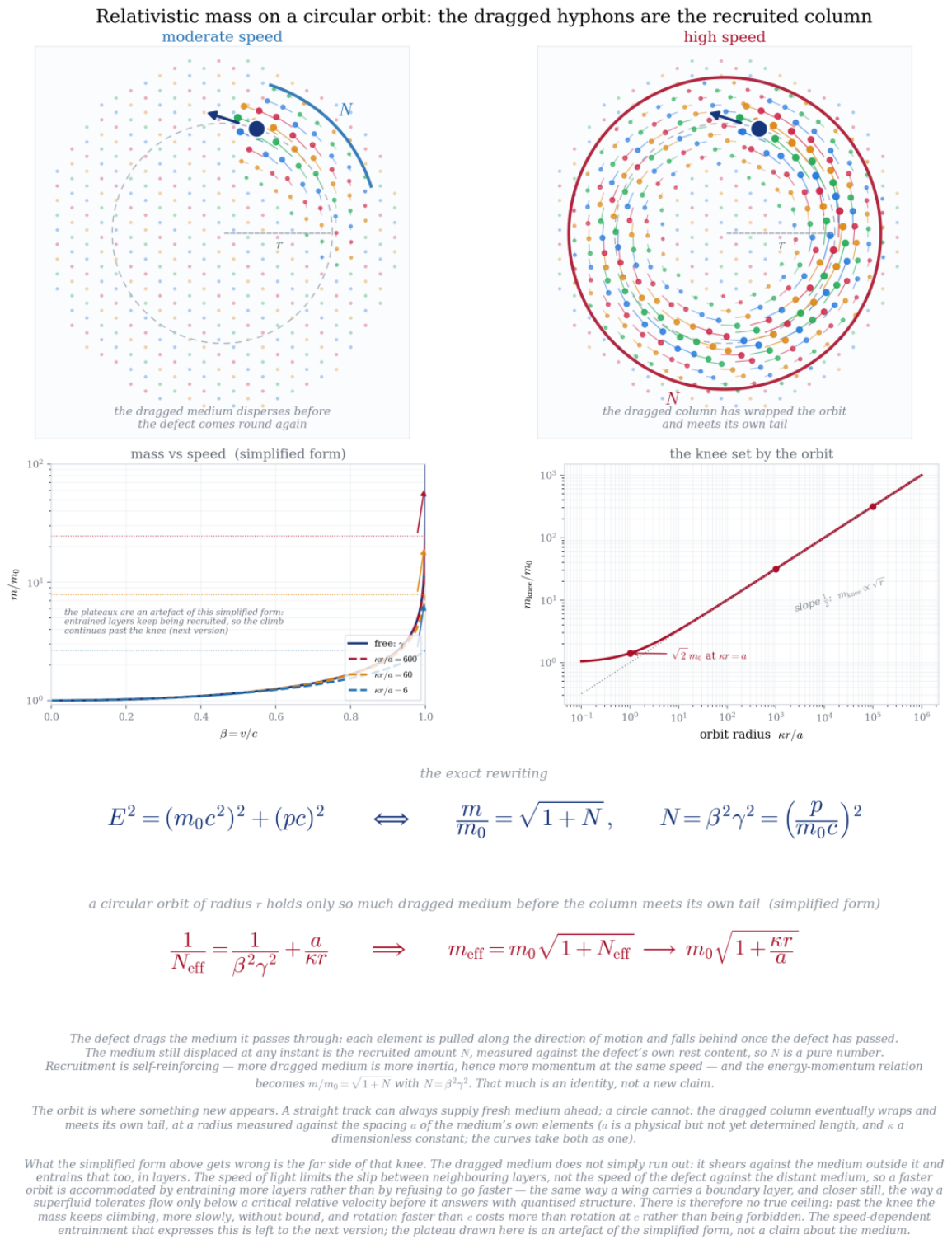
Disclaimer/Publisher’s Note: The statements, opinions and data contained in all publications are solely those of the individual author(s) and contributor(s) and not of MDPI and/or the editor(s). MDPI and/or the editor(s) disclaim responsibility for any injury to people or property resulting from any ideas, methods, instructions or products referred to in the content. |
© 2026 by the authors. Licensee MDPI, Basel, Switzerland. This article is an open access article distributed under the terms and conditions of the Creative Commons Attribution (CC BY) license (http://creativecommons.org/licenses/by/4.0/).
Copyright: This open access article is published under a Creative Commons CC BY 4.0 license, which permit the free download, distribution, and reuse, provided that the author and preprint are cited in any reuse.


