

Submitted:
05 April 2026
Posted:
06 April 2026
You are already at the latest version
Abstract
The Bhatnagar-Gross-Krook (BGK) model in the lattice Boltzmann method (LBM) is being widely used for simulating fluid flow and heat transfer due to its simplicity and parallelization capability. However, improving its computational efficiency and accuracy remains an ongoing challenge. This work introduces a time-averaged equilibrium distribution function (TAE) within the BGK model of collision operator in LBM, aiming to explore its performance in heat diffusion and compressible flows, such as the Sod shock tube. The TAE-LBM is tested on the heat diffusion problem using different values of the numerical relaxation coefficient, and the results show that convergence is achieved with significantly fewer time steps compared to standard LBM and the finite difference method (FDM), while maintaining reasonable accuracy. Higher coefficient values improve accuracy but reduce convergence speed. In Sod shock tube simulation, the TAE approach achieves the lowest root mean square error (RMSE) compared to the finite volume method using the Harten-Lax-van Leer scheme with monotonic upstream-centred for conservation laws reconstruction (FVM-HLL-MUSCL) both first-order Runge-Kutta and second-order Runge-Kutta.
Keywords:
time averaged equilibrium distribution function
; heat diffusion
; sod shock tube
1. Introduction
The computational method for solving engineering problems has become a powerful tool to explore and investigate chemical and physical phenomena. In 1956, the finite element method (FEM) was applied to solve a structural problem by Turner et al., [1]. At the same time the FDM and FEM were used to solve partial differential problems, heat transfer and fluid dynamics problems [2]. The finite volume method was introduced by Imperial College in 1980 to solve transport phenomena problems [3]. All of the aforementioned methods belong to the same family of weighted residual methods, and the only difference between these methods is the base and weight function [4]. The LBM emerged in 1988 to overcome the limitation of the lattice gas cellular automata [5], since then the LBM evolved as an alternative powerful method for solving fluid dynamic problems due to its kinetic-theory foundation, parallelizability, and algorithm simplicity [6,7], the main difficulty in LBM is the collision operator. The simplest approximation of the collision operator without producing significant error outcomes was introduced by Bhatnagar, Gross and Krook.
Over the past two decades, many modifications to the standard LBM have been proposed to improve accuracy, stability and applicability to capture complex flows such as the multiple relaxation time (MRT) has been introduced to reduce the numerical instability in compressible and turbulent flows, as demonstrated in previous studies [8,9,10]. the two-relaxation time model (TRT) was introduced as a simplified variant to balance between performance and efficiency by using two relaxation parameters symmetric and antisymmetric components [11]. In 1999, the Entropic LBM (ELBM) was introduced by Karlin et al., [12], to improve the stability in turbulent and high-speed flows. Cascade LBM, which is known as a central moment method, reformulates the collision using central rather than raw moments to improve Galilean invariance and accuracy. This advancement was achieved by altering the physical model of LBM and the collision structure [13].
There remains a lack of focused research on modifying the equilibrium distribution function in the BGK model by using a time-averaging technique, and on investigating the effect of this averaging on the behavior of the heat diffusion and more broadly, diffusion-type equations, the idea of transforming the FVM into a BGK-like LBM structure, combined with time averaging of the equilibrium distribution function to enable efficient parallelization using the Message Passing Interface with Compute Unified Device Architecture MPI-CUDA, has not yet been explored.
The significance of this study lies in introducing a hybrid modelling approach that bridges numerical formulation and computational implementation. By combining time averaging with BGK and leveraging structural transformation, the work offers a new direction for scalable and stable simulation in both diffusive and compressible regimes.
Therefore, the objective of this study is to propose a novel time-averaged formulation of the equilibrium distribution function within the BGK collision model of the LBM, the aim is to reduce the number of time steps required for the outcomes while maintaining the accuracy, this can be validated through two domains. First, heat diffusion to assess the performance in parabolic transport regime, second the sod shock tube is employed to assess the method’s behavior in compressible flow regime by transforming the mathematical formulation of FVM into an equivalent LBM framework, focusing on preserving the mathematical structure and numerical behavior rather than replicating the physical modeling.
2. Methodology
This study starts from the conventional heat diffusion equation without source term. The equation is first discretized using an explicit FDM approach, employing a forward difference in time and a central difference in space. The discrete form is then compared with LBM formulation with BGK approximation, to establish a connection between the two methods, a mathematical technique is applied to resemble the LBM with the BGK approximation from the FDM, once this resemblance is achieved, we introduce the new formulation of the equilibrium distribution function based on time averaging.
This approach needs information from a future time step, which we don’t have it directly, to overcome this, the standard BGK model is used to estimate the future state, which is then used to recalculate the time-averaging equilibrium distribution function.
A flow diagram is provided to illustrate the proposed computational process, this approach is first tested on the heat diffusion problem and then extended to Sod shock tube, where specific mathematical transformations are applied to the FVM to transform it into BGK-like relaxation form.
Finally, numerical results are generated and compared against conventional methods to assess the performance of the proposed model. Figures are used to visualize the difference and evaluate the effectiveness of the time-averaged equilibrium approach in both diffusive and compressible regimes.
2.1. Governing Equation
We start with the conventional heat diffusion equation in one dimension, without a source term:
where is the temperature, is time, is the spatial coordinate, and is the thermal diffusivity. This equation is discretized using an explicit FDM, employing a forward difference in time and a central difference in space:
where is the spatial node index.
The LBM for heat diffusion equation using BGK approximation can be written as follows:
where is the distribution function in direction , is the lattice velocity, is the relaxation time, is the equilibrium distribution function, is the time step. We rearrange the terms in Eq. (2) to match the structure in Eq. (3) and extract the analogy between the two formulations (Mohamad 2011).
2.2. Resembling Procedure
The Eq. (2) can be written as follows:
Assume:
Substituting Eq. (5) into Eq. (4) gives:
This mathematical manipulation to compare the FDM with LBM approximation of heat diffusion, the last term in Eq. (5) represents the spatially averaged temperature around , because lies at the mid-distance between and , in other word this is the equilibrium value of the , Eq. (6) can be rewritten as follows:
where is the equilibrium value of the temperature at specific location and time . By comparing Eq. (7) and (3) we can assume the is an average value around and lies at the mid-distance between , this analogy is very important for the current study, as it supports the next assumption, which will be the pillar of this work.
2.3. Time-Averaged Equilibrium Distribution function
We propose a new form of the equilibrium distribution function, averaged overtime:
This approach assumes knowledge of future value of , which are not directly available. To resolve this, we first compute the standard BGK solution at , then use the result to reconstruct the time-averaged equilibrium.
2.4. Computational Flow Process
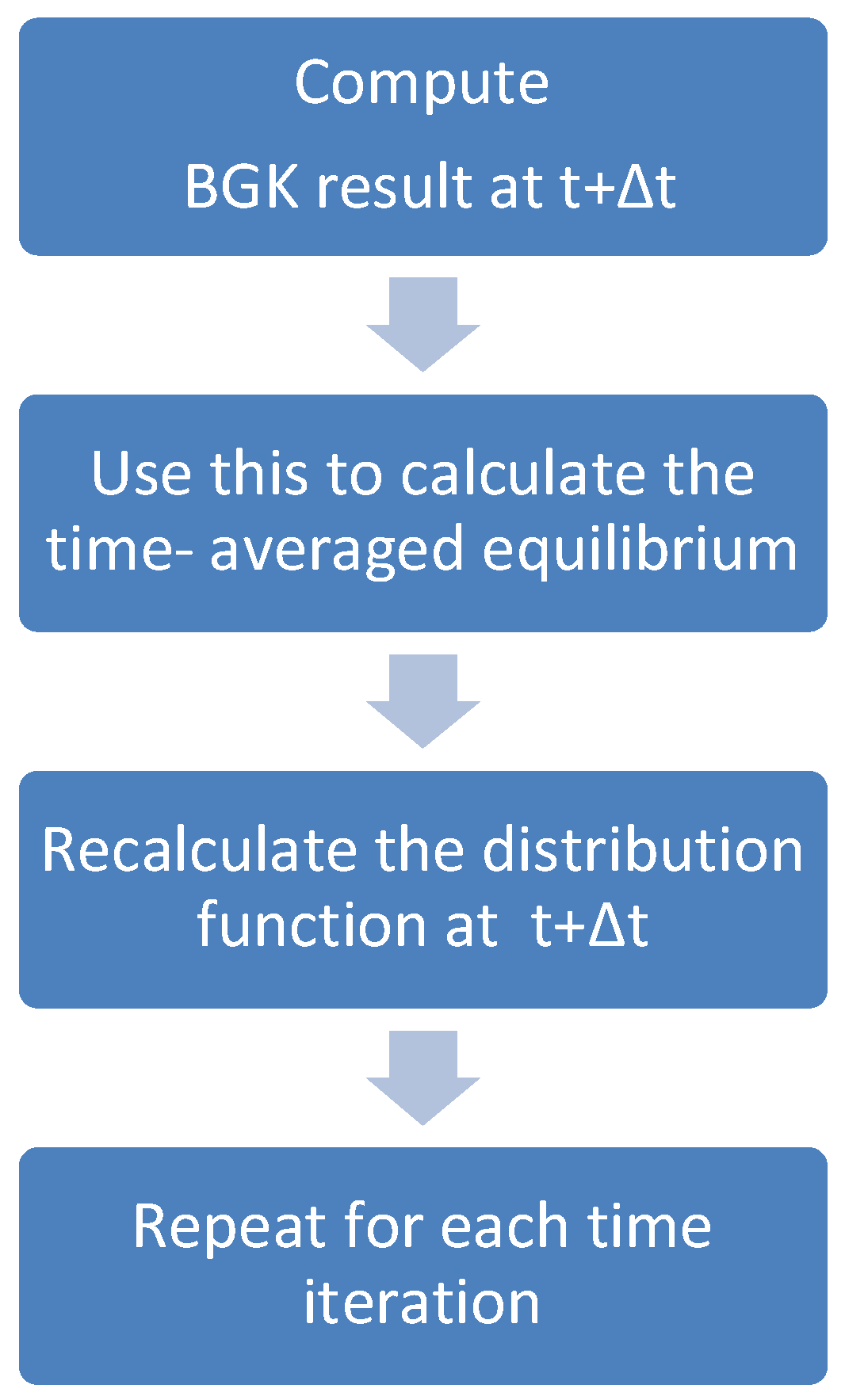
A flow diagram is constructed to summarize the step-by-step process of implementing the time-averaged equilibrium in the BGK model, the process starts with computing the BGK result at , followed by calculating the time-averaged equilibrium, updating the solution and iteration.
Figure 1.
Computational flowchart illustrating the time-averaged BGK procedure used in this study.
2.5. Time-Averaged BGK Formulation for Heat Diffusion
We consider the heat diffusion equation modeled using the LBM with the BGK approximation. The chosen lattice structure is D1Q2, the simulation is conducted in lattice units, where both the spatial and temporal resolutions are normalized to unity. Under this assumption, the discrete velocity set for D1Q2 model is defined as:
Substituting Eq. (9) into Eq. (3) leads to:
where:
The macroscopic temperature is calculated as the sum of two particles populations:
For D1Q2 the equilibrium functions are defined as:
The reformulated LBM with time-averaged can be expressed as follows:
The effective values of in the reformulated LBM cannot be determined analytically; instead, they serve as numerically determined relaxation parameters that governs the rate of convergence, similar in role to the conventional relaxation time in the standard BGK model. To reflect the structural similarity of the reformulated approach with FDM and LBM, we assume
Since future values of the distribution functions are not known in advance, we first use Eq. (10) and Eq. (11) to calculate the future values, then, we substitute these values into Eq. (15) and Eq. (16) to rebuild the updated distribution functions , this sequence is illustrated in the computational flowchart Figure 1.
The D1Q2 lattice is selected in this study due to its minimal complexity, which allows for isolating and evaluating the effect of the proposed time- averaged equilibrium strategy without the influence of higher-order lattice dynamics. The simulation domain is initialized with a uniform temperature of 0 (in lattice unit). Dirichlet boundary conditions are applied at both ends of the domain: the left boundary is fixed at a temperature of 1, while the right boundary is fixed at a temperature of 0 unity. The thermal diffusivity , the length of bar is and for FDM and 100 lattice nodes for LBM.
2.6. Mathematical Formulation and Finite Volume Discretization of the Sod Shock Tube
The Sod shock tube problem is a classical benchmark for evaluating the performance of numerical methods in compressible flows. It is governed by the Euler equations, which explain the conservation of mass, momentum, and energy in an inviscid fluid. In this study, gravitational force and other body forces are neglected, as the flow is assumed to be driven purely by pressure discontinuity.
For the two-dimensional case, the Euler equations can be written in conservative form as:
where the conserved variable vector, and the flux vectors and , are:
The system consists of four variables: represents the density, is the velocity in the x direction, represents the velocity in y direction, represents the energy, represents the pressure. to make it solvable, an additional relation is needed, this is provided by the equation of state.
where represents the specific heat ratio.
The standard FVM discretization of this equation for cell is given by:
Where n represents the time step, in this study, the numerical flux at cell interface is evaluated using HLL approximate Riemann solver, combined with a MUSCL scheme, as proposed in previous studies [14,15], the resulting flux at the cell interface is expressed as:
where and are reconstructed left and right states at the interface and is the centre of the cell, obtained by MUSCL scheme. Eq. (21) can be approximated using the second-order Runge-Kutta method. First, the slope is calculated at the first-time step using the conservative variable values. This slope is then used to extrapolate the conservative variables forward by one time step. Using the extrapolated values, a second slope is computed at the new conservative variable values, as follows:
Eq. (23) represent the first order Runge-Kutta method, where represents the slope at the initial time, this equivalent to the explicit Euler method and serves as a basic time integration scheme, to extrapolate the conservative variable at next time step:
The slope at next time step can be obtained by:
Reupdate the conservative variable by averaging the slopes as follows:
Eq. (26) represents the second order Runge-Kutta method, improving the accuracy of the time integration. The second order scheme along with the first order will be used as a base line for comparison, in this study the result from the four approaches will be compared: the analytical solution, the first order finite volume method, the second order Runge-Kutta method and the proposed time-averaged BGK.
2.7. Transformation of FVM-HLL-MUSCL into a BGK-like Relaxation Form
To enable a BGK-style relaxation approach in the context of FVM, we start from the classical 2D explicit finite volume update for the conserved variables. The update equation for a control volume at is given by:
Sum Eq. (28) with Eq. (21), rearrange it in term of :
Assume:
Leads to:
We can repeat the same procedure for , the resultant equations are:
The same procedure for :
To construct a BGK-like analogy D2Q4, we define pseudo distribution functions:
And:
The transformation of the LBM with time-averaged formulation can be expressed as follows:
where and are numerical coefficients. In this study, we set and , to maintain structural consistency. These reconstructed forms of the update equations enable the application of the time-averaged equilibrium formulation, as previously discussed.
2.8. Parallelization Compatibility
The reformulated equations, expressed in a BGK-like relaxation form with a time-averaged equilibrium function, is particularly well-suited for parallel implementation. Since the update at each lattice node relies only on its immediate neighbours and the equilibrium distribution, the method permits efficient domain decomposition and parallel execution. This locality makes it highly compatible with MPI for distributed memory systems and CUDA for GPU acceleration, enabling scalable performance on high-performance computing platforms.
2.9. Sod Shock Tube Configuration and Analytical Reference
The Sod shock tube is initialized with a partition at the centre of the domain. The left state is defined as and the right state is defined as , the ratio of the specific heat is set to , where R and L represent right and left respectively.
The analytical solution for the sod shock tube is available from Riemann problem for the Euler equations, as described by Toro [16], this solution is used as a benchmark to validate the numerical results presented in this study.
3. Results
3.1. Heat Diffusion
To evaluate the performance of the proposed time-averaged equilibrium LBM (TAE-LBM) on heat diffusion equation, two benchmark simulations were used and compared with the FDM, the focus is on two parameters: the number of time steps needed to simulate a fixed physical time and the solution accuracy, calculated by root mean square error RMSE. Additionally, observations from additional runs using extreme values of relaxation coefficient to assess the stability of the TAE-LBM under varying relaxation conditions.
3.1.1. Simulation 1
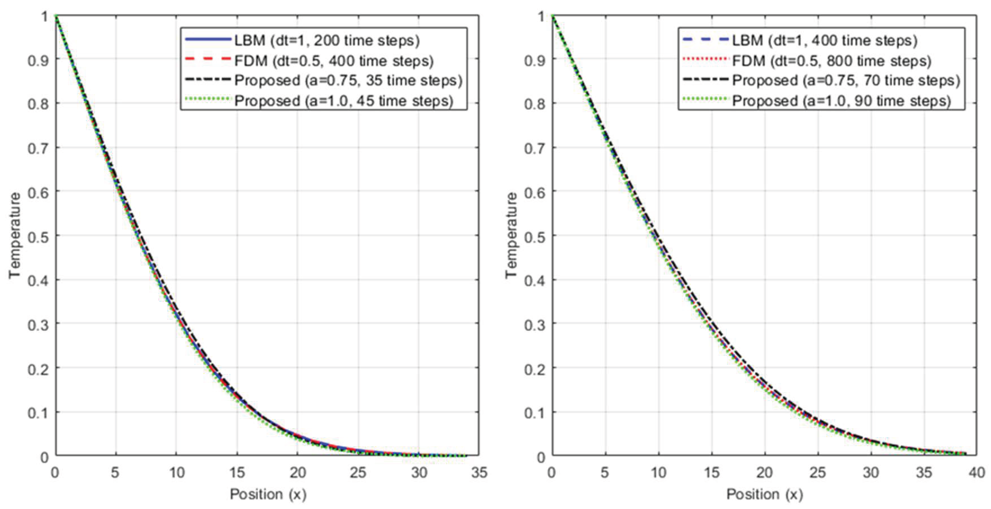
In the first simulation, the temperature distribution was observed over a short physical duration, as shown in Table 1 and Figure 2, FDM required a 400 time-steps with while the LBM completed the same simulation in 200 time-steps.
TAE-LBM, calculated for two coefficients and , needed 35 time-steps and 45 time-steps, respectively, the standard LBM produced the lowest RMSE, indicating the highest accuracy among all methods, TAE-LBM with produced the highest RMSE, while LBM with showed better accuracy than LBM with , indicating that the accuracy improve as increases.
3.1.2. Simulation 2
In the second simulation, the temperature distribution was observed over a longer physical duration, as shown in Table 1 and Figure 2, FDM required 800 time-steps with and LBM required 400 time-steps, TAE-LBM performed consistently, finished the simulation in 70 time-steps for and 90 for .
Accuracy stayed similar, LBM produced the lowest RMSE, followed by TAE- LBM with and , again, the accuracy improved as increased.

Table 2.
Convergence and accuracy in simulation 2.
| Simulation 2 | FDM dt=0.5 | LBM | TAE-LBM a=0.75 | TAE-LBM a=1 |
|---|---|---|---|---|
| Number of time steps |
800 | 400 | 70 | 90 |
| RMSE | 0.00031 | 0.006159 | 0.00303 |
3.1.3. Visual Analysis
Figure 2 presents the temperature distribution results from Simulations 1 and 2. In both simulations, the TAE-LBM curves closely follow the FDM and LBM results. The TAE-LBM with a=1 consistently gives better convergence and lower RMSE than TAE-LBM with a=0.75, as it reduces to a purely time-averaged equilibrium that depends only on the equilibrium distribution function, both simulations, however, use fewer time-steps than LBM and FDM, lowering the value of a results in faster convergence, but at the cost of accuracy.
Figure 2.
Comparison of spatial temperature distributions using LBM, FDM, and time-averaged equilibrium method with its proposed coefficient (a) are compared at two different simulation times.
Figure 2.
Comparison of spatial temperature distributions using LBM, FDM, and time-averaged equilibrium method with its proposed coefficient (a) are compared at two different simulation times.
3.1.4. Extreme Coefficient Values
Additional test with extreme values of showed limitations of TAE-LBM at , the solution remains static, showing no diffusion. At the solution becomes unstable with non-physical values. these observations lead to the definition of the valid domain as 1.2<a>0.
3.2. Sod Shock Tube
The Sod shock tube problem was simulated to evaluate the accuracy of different numerical methods at t=0.2 s. Figure 3 presents the density distribution for three different numerical methods FVM-HLL-MUSCL scheme with first order Runge-Kutta, FVM-HLL-MUCSLE with second order Runge-Kutta and TAE-BGK-like relaxation form. These are compared against the analytical solution. The first-order FVM produces noticeable diffusion and oscillations near the shock discontinuity. In contrast, the second-order FVM and the BGK-like relaxation form solved by TAE-LBM capture the discontinuity with improved accuracy.
Table 1 lists the RMSE for each method. The TAE-BGK-like relaxation form achieved the best result with the analytical solution.
Table 3.
RMSE of density for different methods.
| Simulation 3 | Analytical Solution | FVM first order | FVM second order | BGK-like relaxation form |
|---|---|---|---|---|
| RMSE | 0.02809 | 0.01639 | 0.015134 |
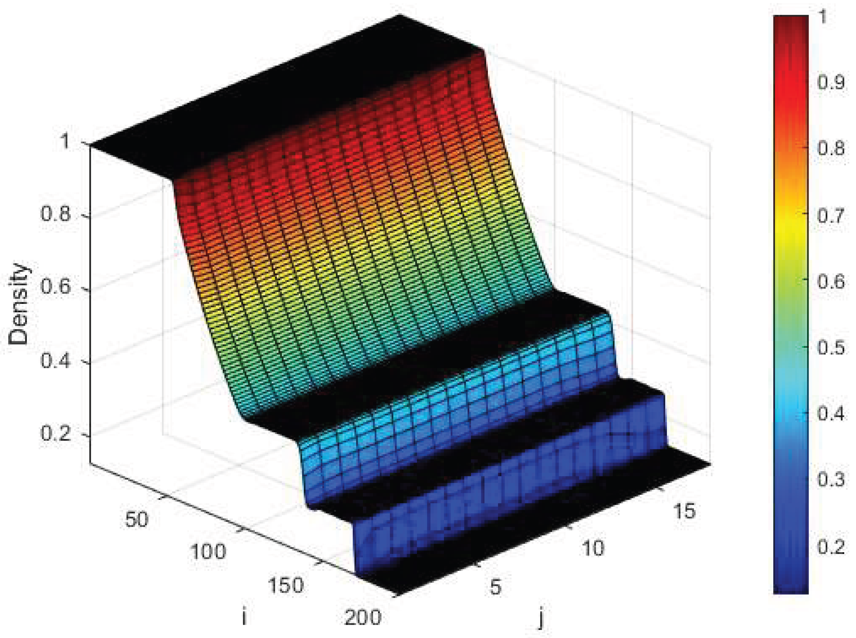
In addition to the 1D results, a 2D simulation was produced using the TAE-LBM method:
Figure 4.
Figure 4 shows the density profile comparison at for the Sod shock tube problem in 2D.
Figure 4.
Figure 4 shows the density profile comparison at for the Sod shock tube problem in 2D.
4. Conclusions
A new method, the Time-Averaged Equilibrium Lattice Boltzmann Method (TAE-LBM), was introduced and investigated by two benchmark simulations: the heat diffusion and Sod shock tube problem. In heat diffusion TAE-LBM achieved faster convergence with significantly fewer number of time steps compared with LBM and FDM, but with less accuracy than other methods, increasing the value of a leads to increased accuracy and a decrease in the number of time steps to converge, a trade-off between stability and precision, while the extreme value of a highlights the method’s limitations, determining a valid operational range. In Sod shock tube, when TAE-LBM was applied on the BGK-like relaxation form, it showed a good agreement in terms of accuracy, no reduction or increase in the number of time steps. Overall, TAE-LBM presents an efficient direction for efficient and accurate numerical simulations, with potential for further optimization and extension.
Author Contributions
Writing – original draft, Wasif M Almady; Supervision, Antonis Papadakis. All authors have read and agreed to the published version of the manuscript.
Funding
This research received no external funding.
Data Availability Statement
The original contributions presented in this study are included in the article. Further inquiries can be directed to the corresponding author(s).
Acknowledgments
The authors acknowledge A.A. Mohamad's comments and discussions during the revision of the manuscript. Also, his textbook on Lattice Boltzmann Methods was instrumental to our fundamental understanding of LBM..
Conflicts of Interest
The authors declare no conflict of interest.
References
- Turner, M. Jon, Ray W. Clough, Harold C. Martin, and L. J. Topp. "Stiffness and deflection analysis of complex structures." journal of the Aeronautical Sciences 23, no. 9 (1956): 805-823. .
- Mohamad, A. A. Lattice boltzmann method. Vol. 70. London: Springer, 2011.
- Spalding, D. B. "Mathematical modelling of fluid-mechanics, heat-transfer and chemical-reaction processes." A Lecture Course, Imperial College CFDU Report (1980).
- Chen, Shiyi, and Gary D. Doolen. "Lattice Boltzmann method for fluid flows." Annual review of fluid mechanics 30, no. 1 (1998): 329-364. [CrossRef]
- He, Xiaoyi, and Li-Shi Luo. "Lattice Boltzmann model for the incompressible Navier–Stokes equation." Journal of statistical Physics 88 (1997): 927-944. [CrossRef]
- Lallemand, Pierre, and Li-Shi Luo. "Theory of the lattice Boltzmann method: Dispersion, dissipation, isotropy, Galilean invariance, and stability." Physical review E 61, no. 6 (2000): 6546. [CrossRef]
- Aidun, Cyrus K., and Jonathan R. Clausen. "Lattice-Boltzmann method for complex flows." Annual review of fluid mechanics 42, no. 1 (2010): 439-472. [CrossRef]
- Jahanshaloo, L., NA Che Sidik, and S. Salimi. "Numerical simulation of high Reynolds number flow in lid-driven cavity using multi-relaxation time Lattice Boltzmann Method." Journal of Advanced Research in Fluid Mechanics and Thermal Sciences 24, no. 1 (2016): 12-21. [CrossRef]
- d'Humières, Dominique. "Multiple–relaxation–time lattice Boltzmann models in three dimensions." Philosophical Transactions of the Royal Society of London. Series A: Mathematical, Physical and Engineering Sciences 360, no. 1792 (2002): 437-451. [CrossRef]
- Asinari, Pietro. "Multiple-relaxation-time lattice Boltzmann scheme for homogeneous mixture flows with external force." Physical Review E—Statistical, Nonlinear, and Soft Matter Physics 77, no. 5 (2008): 056706. [CrossRef]
- Ansumali, Santosh, and Iliya V. Karlin. "Single relaxation time model for entropic lattice Boltzmann methods." Physical Review E 65, no. 5 (2002): 056312. [CrossRef]
- Hosseini, Seyed Ali, Mohammad Atif, Santosh Ansumali, and Iliya V. Karlin. "Entropic lattice Boltzmann methods: A review." Computers & Fluids 259 (2023): 105884. [CrossRef]
- Krüger, Timm, Halim Kusumaatmaja, Alexandr Kuzmin, Orest Shardt, Goncalo Silva, and Erlend Magnus Viggen. "The lattice Boltzmann method." Springer International Publishing 10, no. 978-3 (2017): 4-15. [CrossRef]
- Li, Zheng, Mo Yang, and Yuwen Zhang. "A hybrid lattice Boltzmann and finite-volume method for melting with convection." Numerical Heat Transfer, Part B: Fundamentals 66, no. 4 (2014): 307-325. [CrossRef]
- Davis, Stephen F. "Simplified second-order Godunov-type methods." SIAM Journal on Scientific and Statistical Computing 9, no. 3 (1988): 445-473.
- Toro, Eleuterio F., Michael Spruce, and William Speares. "Restoration of the contact surface in the HLL-Riemann solver." Shock waves 4, no. 1 (1994): 25-34.
Figure 3.
Figure 3 shows the density profile comparison at t=0.2 s for the Sod shock tube.
Figure 3.
Figure 3 shows the density profile comparison at t=0.2 s for the Sod shock tube.
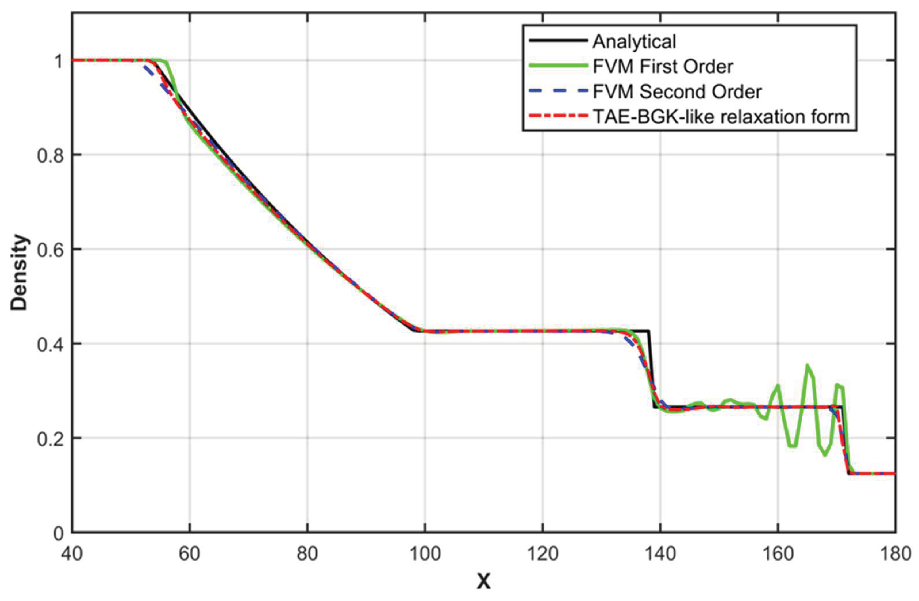
Table 1.
Convergence and accuracy in simulation 1.
| Simulation 1 | FDM dt=0.5 | LBM | TAE-LBM a=0.75 | TAE-LBM a=1 |
|---|---|---|---|---|
| Number of time steps |
400 | 200 | 35 | 45 |
| RMSE | 0.000524 | 0.005569 | 0.00324 |
Disclaimer/Publisher’s Note: The statements, opinions and data contained in all publications are solely those of the individual author(s) and contributor(s) and not of MDPI and/or the editor(s). MDPI and/or the editor(s) disclaim responsibility for any injury to people or property resulting from any ideas, methods, instructions or products referred to in the content. |
© 2026 by the authors. Licensee MDPI, Basel, Switzerland. This article is an open access article distributed under the terms and conditions of the Creative Commons Attribution (CC BY) license (http://creativecommons.org/licenses/by/4.0/).
Copyright: This open access article is published under a Creative Commons CC BY 4.0 license, which permit the free download, distribution, and reuse, provided that the author and preprint are cited in any reuse.


