Within-Venue Monitoring of BTC/USDT Liquidity and Resiliency on Binance: A Queueing-Theoretic Framework

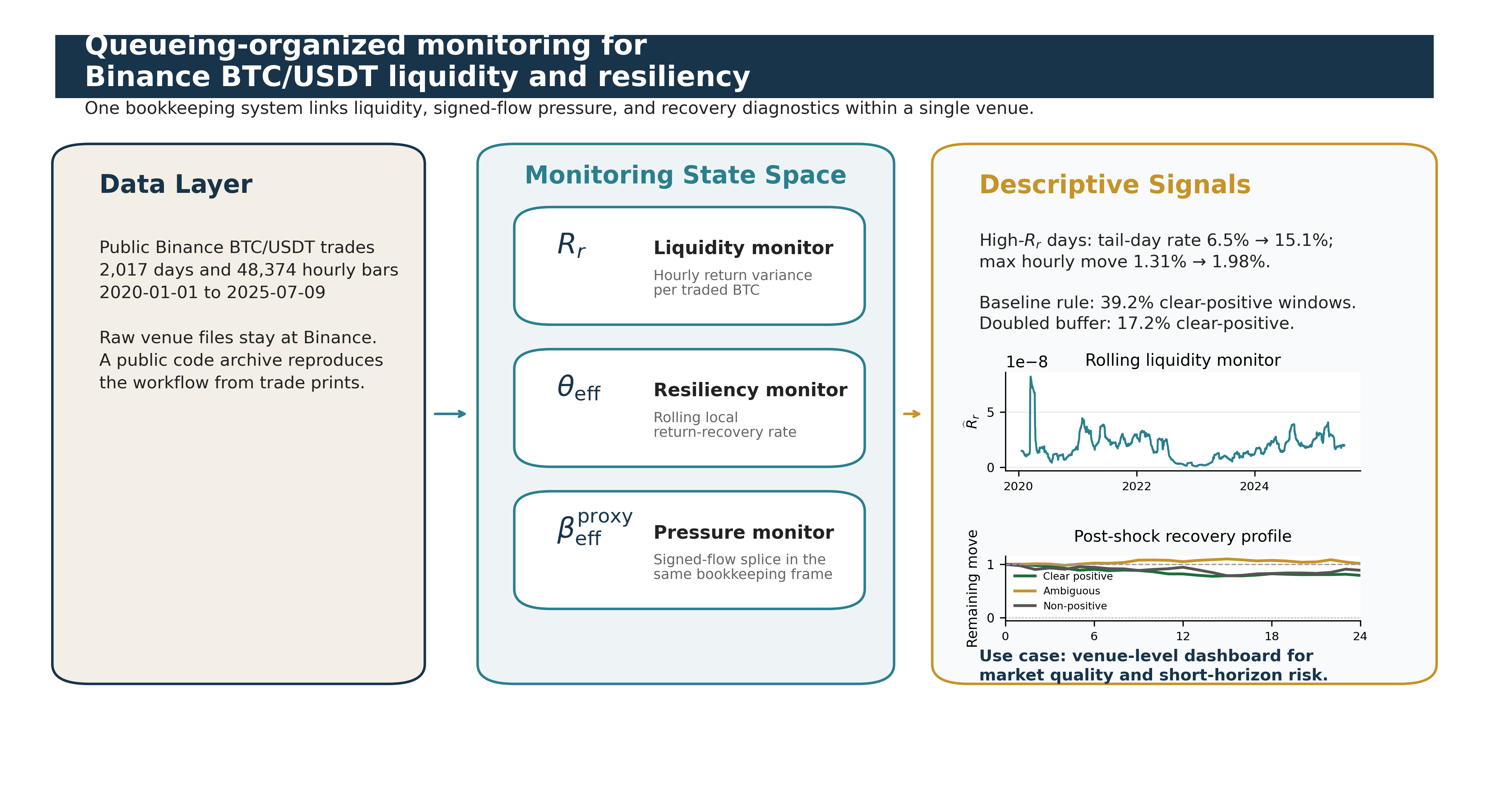
We develop a queueing-organized framework for within-venue monitoring of BTC/USDT liquidity, signed-flow pressure, and resiliency on Binance. The model treats latent buy and sell pressure as occupancy processes and uses that state space to organize three empirical diagnostics: the variance-per-BTC liquidity measure R_r, the effective mean-reversion rate θ_eff, and the companion signed-flow proxy beta^proxy_eff. Using Binance trade data from 2020 to 2025, we find a pooled first-order variance-volume regularity away from the highest-volume tail and substantial time variation in rolling liquidity and resiliency. In overlapping 30-day windows, θ_eff is positive by point estimate in roughly two-thirds of windows but clearly positive in only about two-fifths under a simple uncertainty buffer, implying that local recovery is often fragile or ambiguous. The intended users are short-horizon risk managers, execution desks, market makers, and exchange surveillance teams that need auditable venue-level indicators of when liquidity is thinning, recovery is weakening, and signed flow is turning one-sided. Queueing is useful here because it turns those signals into one coherent monitoring dashboard for venue-level market quality and short-horizon risk.