Submitted:
31 March 2026
Posted:
01 April 2026
You are already at the latest version
Preprints on COVID-19 and SARS-CoV-2
Abstract
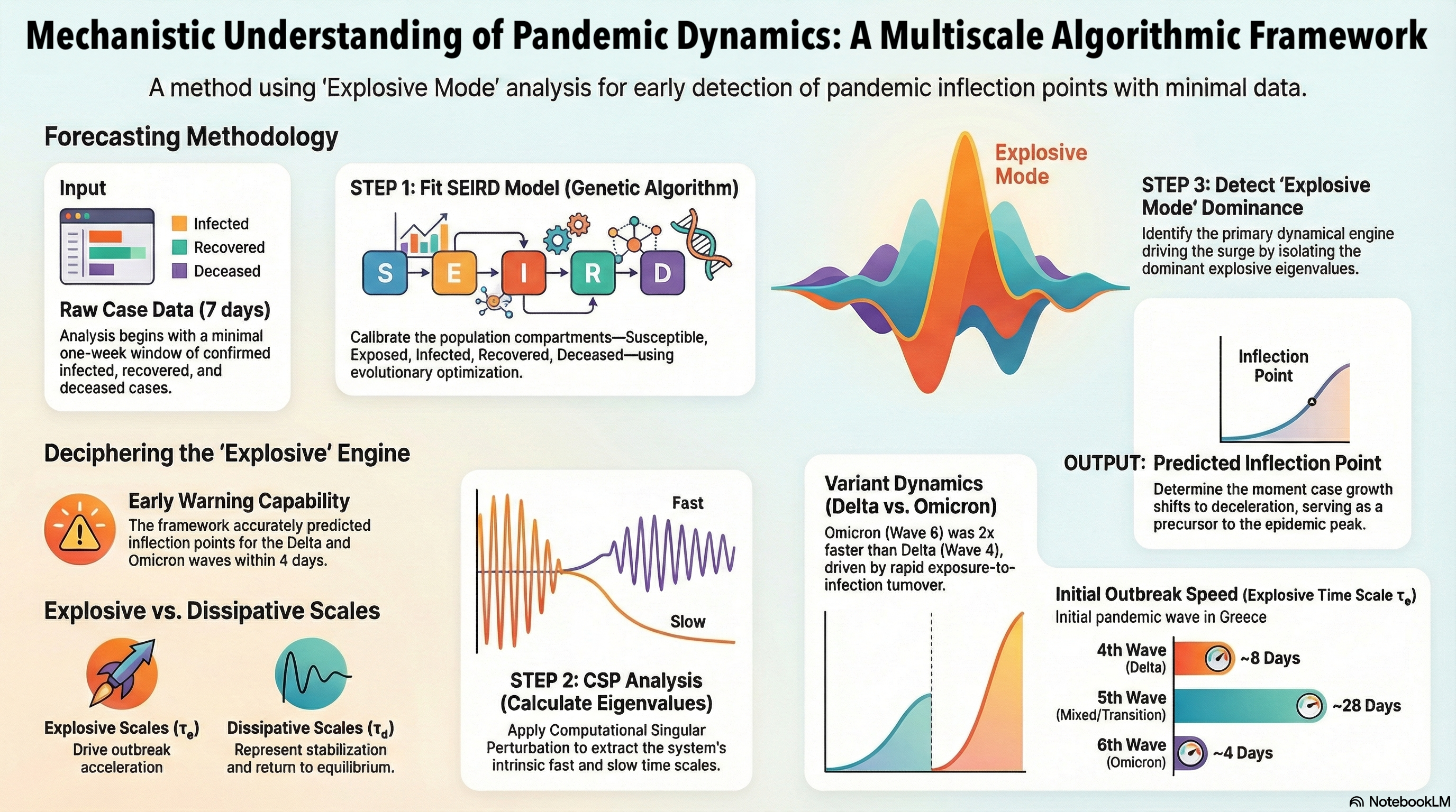
We present a robust, data-efficient framework for early outbreak assessment using multiscale analysis and Computational Singular Perturbation (CSP). This framework overcomes the shortcomings of the standard compartmental epidemiological models, which often struggle with parameter identifiability during the early stages of a pandemic, limiting considerably their predictive utility when data is sparse. Rather than relying on curve-fitting population profiles, which are sensitive to uncertainty, our approach isolates the dominant "explosive" time scale that characterizes the outbreak’s intensity and duration. Using a calibrated SEIRD model, CSP allows for the identification of the paths that drive the process during the outbreak phase and the critical transition from accelerating to decelerating growth, which serves as a reliable precursor to the epidemic peak. This framework is assessed against the 4th, 5th, and 6th waves of the COVID-19 pandemic in Greece during 2021, covering periods dominated by the Delta and Omicron variants. Using only early-stage data from short calibration windows, CSP diagnostic tools revealed distinct dynamical drivers for each wave; e.g., a transition from the 4th wave that was driven by transmission intensity (Delta variant dominance) to the 6th wave that was driven by rapid exposure-to-infection turnover and reduced opposition from recovery mechanisms (Omicron variant dominance). Furthermore, it is demonstrated that the timing of outbreak’s weakening can be accurately predicted, demonstrating robustness with results obtained from longer observation windows. These findings position multiscale analysis as a powerful, pathogen-agnostic early-warning system, capable of disentangling complex epidemic mechanisms and assessing intervention efficacy in real-time.
Keywords:
predictive models of pandemics
; COVID-19
; population dynamics
; time scale analysis
; computational singular perturbation
1. Introduction
Pandemics have historically posed critical challenges to global public health, prompting extensive efforts across the mathematical and computational sciences to model, understand, and predict their progression. The COVID-19 pandemic, which began in late 2019, intensified this research, with early studies focusing on characterizing the initial outbreak dynamics [1,2,3], performing comparative analyses across countries [4,5,6], and examining spatial transmission patterns within national and regional settings [7,8]. As the pandemic progressed, attention focused toward quantifying the effectiveness of non-pharmaceutical interventions [9,10,11], mitigating healthcare system overload [12,13,14], and designing optimal exit strategies [15,16,17]. Throughout all stages, predictive modeling of epidemic trajectories and real-time estimation of the reproduction number remained central objectives [18,19,20].
This sustained research effort has produced a wide array of mathematical modeling approaches. Ordinary differential equation (ODE) compartmental models remain foundational [21,22,23,24], complemented by agent-based models [6,25,26] and meta-population formulations [27,28,29]. In parallel, data-driven approaches including machine learning [30,31], deep learning [32,33,34], Bayesian inference, and autoregressive time-series techniques [35,36,37] have been increasingly adopted. Systematic reviews of early COVID-19 forecasting efforts highlight both the breadth of methodologies employed and the substantial uncertainty associated with early predictions [38,39,40].

Table 1.
Translational Glossary: Mapping Computational Singular Perturbation (CSP) terminology to biological and epidemiological interpretation.
Table 1.
Translational Glossary: Mapping Computational Singular Perturbation (CSP) terminology to biological and epidemiological interpretation.
| Mathematical Term (CSP) | Biological / Epidemiological Translation | Practical Significance in This Study |
| Mode () | Dynamical component | A component of the model, the action of which is characterized by an explosive or dissipative time scale. The mode that is characterized by the fastest time scale drives the initial surge, while all other modes sustain or attenuate the epidemic wave before stabilization occurs. |
| Explosive Time Scale () | Characteristic expansion time | Represents the time frame of the action of a mode (explosive) that tends to drive the system away from equilibrium. A smaller value (e.g., ∼4 days during the 6th wave) indicates a more aggressive and rapidly spreading variant compared to larger values (e.g., ∼8 days during the 4th wave or ∼28 days during the 5th wave). |
| Dissipative Time Scale () | Stabilization or damping rate | Represents the time frame of the action of a mode (dissipative) that tends to drive the system towards equilibrium. When a dissipative mode dominates, the outbreak transitions into decay and active cases begin to decline. |
| Slow Invariant Manifold (SIM) | Epidemic trajectory | The reduced-dimensional path followed by the epidemic once fast transient processes subside. It represents the established dynamical regime during the outbreak phase. |
| Amplitude (f) | Driver intensity | Provides a measure of the impact of a mode in driving the epidemic wave. In the case of an explosive mode, a high amplitude indicates dominant transmission dynamics, while a low amplitude signals increasing control or immunity effects. |
| Time Scale Participation Index (TPI) | Mechanism identifier | Quantifies the contribution of individual biological transitions (e.g., transmission, incubation, recovery) to the time scale. In the case of an explosive time scale, it determines the degree to which the outbreak is promoted by high transmission () or by rapid progression from exposure to infection (), or it is obstructed by recovery (). |
| Pointer (Po) | Population influence index | Identifies which population compartment most strongly influenced by a specific mode. For example, a high Pointer value for the exposed population during the 6th wave indicates that rapid progression from exposure to infection drives the surge. |
| Inflection Point | Turning point in epidemic acceleration | The moment when outbreak growth shifts from acceleration to deceleration. This precedes the peak of infected population and serves as an early warning indicator of the impending peak. |
Among these approaches, compartmental epidemic models remain the most widely used due to their analytical tractability, interpretability, and ability to incorporate mechanistic understanding of disease transmission. The classical SIR model [41,42] and its extensions can capture key epidemiological characteristics [43,44], including presymptomatic transmission, asymptomatic infections, and disease-induced mortality [45,46]. For COVID-19, SEIRD-type models were shown particularly appropriate due to the presence of an incubation period and non-negligible fatality rates [47,48,49,50]. The SEIRD model has been extended to incorporate vaccination dynamics and intervention measures in order to improve epidemic prediction under evolving public-health conditions [51]. Comparative studies demonstrated that increasing model complexity does not necessarily lead to improved early predictive performance, especially under limited data availability [52].
Early forecasting based on compartmental models demonstrated both their utility and their limitations. While short-term predictions captured initial exponential growth, longer-term forecasts were often highly sensitive to parameter uncertainty and structural assumptions [53]. Parameter identifiability issues are particularly severe during the early outbreak phase, where sparse, delayed, and heterogeneous data lead to multiple parameter sets that fit observations equally well but diverge significantly in their predictions [54,55,56]. These challenges have been documented extensively for COVID-19 [38,57,58]. Hybrid approaches combining mechanistic models with data-driven methods have been proposed to mitigate these issues, though they remained sensitive to reporting delays, intervention changes, and calibration strategies [32,44,59,60,61].
A particularly influential line of work has focused on identifying early dynamical signatures of epidemic transitions. Change-point detection and Bayesian inference techniques have revealed how intervention measures alter transmission dynamics during the early exponential phase [40]. Early warning systems were designed to predict epidemic surges or peaks before they show up in official case data [62,63]. Nevertheless, many of these methods still rely heavily on sufficient observational data and may struggle precisely when early prediction is most critical.
Motivated by the limitations of existing early prediction approaches, and particularly their reliance on extensive parameter calibration and large, high-quality datasets, this work proposes an alternative framework for early pandemic outbreak prediction grounded in time scale analysis of epidemic dynamics. Rather than focusing on solution profiles, which are often highly sensitive to parameter non-identifiability, the proposed approach exploits the intrinsic multiscale structure of compartmental epidemic models. Epidemic systems naturally exhibit processes evolving over multiple time scales, encompassing interactions between transmission, latency, recovery, and population turnover mechanisms [64,65]. By identifying and analyzing the time scales characterizing these interactions, it is possible to infer critical features of outbreak evolution, such as the driving paths, the critical population groups or regime shifts, using limited early-phase data. This time scale–based perspective provides a complementary and data-efficient pathway for early outbreak prediction, strengthening the theoretical foundations of epidemic forecasting and aligning with broader calls for system-oriented modeling frameworks capable of integrating complex epidemic dynamics [66,67].
Herein, the use of Computational Singular Perturbation (CSP) [68,69] is proposed as the core methodological tool for implementing this time scale–based framework in compartmental epidemic models. CSP is an algorithmic method of Geometrical Singular Perturbation Analysis (GSPA), designed for the analysis of multiscale dynamical systems that are driven by processes evolving over widely separated fast and slow time scales. In such systems, processes associated with fast time scales are rapidly equilibrated, leading to the formation of low-dimensional structures in the system’s tangent space, known as Slow Invariant Manifolds (SIMs) [70]. System trajectories subsequently evolve along these manifolds, governed by the remaining slow processes. CSP provides a complete and systematic set of diagnostic tools for identifying (i) the variables and processes associated with fast time scales that generate the SIM and (ii) the slow processes that dominate the long-term system dynamics [71].
Originally developed for the analysis of chemical kinetic mechanisms [72,73], CSP has since emerged as a general framework for multiscale dynamical systems, with applications spanning systems biology [74,75], pharmacokinetics [76,77], brain lactate metabolism [78,79], glycolysis [80] and population dynamics [81].
To demonstrate the systems-level understanding that can be acquired with the proposed CSP–based time scale analysis framework, we apply it to the case of the COVID-19 epidemic in Greece. The analysis will focus on the dynamics of the outbreak of the epidemic wave. Given prior knowledge regarding the existence of a latency period following infection with the SARS-CoV-2 virus [47,48], a SEIRD model is employed, incorporating exposed and deceased population groups. Specifically, we examine the 4th, 5th, and 6th epidemic waves in Greece, which occurred in July 2021, October 2021, and December 2021, respectively. Each wave was driven by different underlying dynamics, reflecting changes in transmission intensity, population behavior, and intervention policies. Using CSP diagnostic tools, we focus on the mode that drives the outbreak and we identify the dominant populations and transition processes governing the outbreak phase of each epidemic wave, based solely on early-stage dynamics and limited observational data. This case study illustrates the method’s ability to disentangle evolving epidemiological mechanisms and highlights its potential as a robust early-warning tool for pandemic outbreak dynamics.
The overall methodological framework adopted in this study is summarized in Figure 1. The flowchart illustrates the sequential procedure from early outbreak data acquisition to CSP-based dynamical analysis and inflection point prediction.
2. Materials and Methods
2.1. The Mathematical Model
According to the SEIRD model, the population of susceptible individuals () might become exposed ones () upon transmission of the virus; i.e., individuals that are infected but not yet infectious. After the incubation period, the exposed individuals become infected (), so they are able to transmit the virus. The infected individual can then either become deceased () or recovered (). The paths that connect the five population groups, according to the SEIRD model, are depicted schematically in Figure 2.
block = [draw=blue, line width=1pt,fill=gray!3, rectangle, minimum height=2em, minimum width=3em] sum = [draw, fill=white!3, stroke=white, circle, node distance=1cm] input = [coordinate] output = [coordinate] pinstyle = [pin edge=to-,thin,blue]
The governing equations of the SEIRD model are:
where is the transmission density-dependent ratio, is the transition ratio from exposed to infected individuals, expressing the inverse of the incubation period of the disease, is the recovery ratio, which also expresses the inverse of the infection period of the disease and is the fatality ratio. Note that , and are decoupled from and . The SEIRD model in Eq. (1) can be cast in the form:
where is the 5-dim. column state vector, the elements of which represent the number of individuals in the population groups; The 5-dim. column vector field incorporates the transition rates from a compartmental group to another. The column vectors (k=1,4) denote the directions of the 5 transitions from a population group to another; , , , . The scalars (k=1,4) are the related to rates of transition; , , and , which denote the transmission, incubation, recovery and death rates, respectively. The model in Eq. (2) is subject to two conservation laws:
2.2. Model Calibration
The model was calibrated against the daily cases of confirmed infected (), recovered () and deceased () individuals, as reported by the Greek government COVID-19 data repository [82]. The initial conditions of the susceptible () and exposed () individuals and the parameter values of , , and were estimated using the Genetic algorithm [83] provided by COPASI [84], on the basis of the reported data sets of , and . Since this study focuses on the outbreak phase of three different epidemic waves, the model was calibrated for two periods of each wave, in order to demonstrate the robustness of the results. The starting point of both periods was the same (the start of the wave), while the end of these periods was different, but within the outbreak phase; see Section 3.1, Section 3.2 and Section 3.3 for details. The parameter values thus estimated for all six periods are displayed in Table 2.
2.3. Modeling Assumptions and Vaccination Effects
It is noted that during the three epidemic waves considered here, vaccination coverage constituted and important factor. The vaccination campaign expanded during the first half of 2021; starting from older populations late January of 2021 and reaching 30-59 years old in April of that year [85]. Therefore, vaccination had no important effect during the 4th wave (July 2021), but had a stronger influence during the 5th and 6th waves (October-November 2021 and December 2021 - January 2022, respectively); although, due to the prevailing Omicron new variant during the 6th wave [86,87], the vaccine might have been not as effective as it was with the Delta variant that prevailed during the 4th and 5th waves [88]. The SEIRD framework employed here does not explicitly include dedicated compartments for vaccinated individuals or waning immunity (i.e., reinfections). This modeling choice was made to preserve structural parsimony and to focus on the dynamical properties of the outbreak phase rather than on detailed population stratification.
Importantly, the CSP-based time scale analysis relies on the local dynamical structure of the system, as encoded in the Jacobian matrix. Consequently, the net effects of vaccination, partial immunity, and reinfection are implicitly reflected in the coefficients of the model. Changes in susceptibility, reduced infectiousness, or accelerated recovery due to vaccination or reinfection manifest as modifications in the coefficients of the transition pathways, which in turn alter the characteristic dynamics. Therefore, while vaccination and reinfections are not modeled explicitly as a separate compartments, their aggregate dynamical impact is captured in the model.
2.4. Time Scale Analysis and CSP Tools
In the Computational Singular Perturbation (CSP) context, Eq. (2) is cast in the form:
where the column CSP vectors (n=1,...,5) span the 5-dim. tangent space, the row vectors are their dual () and the amplitudes are the projections of the vector field on (by proper adjustment of the signs of the CSP basis vectors) [68,69]. Each mode associates with a time scale , ordered so that . The amplitude provides a measure of the impact of the mode, while the time scale provides a measure of the time frame of its action. The time scale can be explosive or dissipative, depending on whether the components of the vector field responsible for its generation tend to move the trajectory away or towards equilibrium [89,90]. Due to the conservation laws in Eq. (3), and . As a result, only the first three modes will be retained in Eq. (4) and the last two will be neglected. According to CSP, the basis vectors are computed via a refinement procedure that provides, order by order, the higher order corrections in the context of asymptotic analysis [91,92].
It will be shown next that during the outbreak phase of all three pandemic waves considered, the fastest time scale is of dissipative character (henceforth, and ), while the other two time scales are of explosive one (henceforth, , and , ); where . Due to the dissipative character of the fastest time scale , the magnitude of the related amplitude is the outcome of significant cancellations among the additive terms in the rhs of its expression:
i.e., , where the magnitude of this ratio is proportional to the ratio [69,91]. As it will be shown next, when the pandemic waves will be analyzed, these cancellations tend to keep the amplitude small, so that the process is mainly driven by the dominant of the two slower explosive modes; see Appendix A for details. Interested in leading order accuracy, the CSP basis vectors can be represented by the right eigenvectors of the Jacobian of ; i.e., and , where and are the right and left eigenvectors of , satisfying [68]. The CSP formulation in the form of Eq. (4) allows the development of various diagnostics tools, among them the Pointer (Po) and the Timescale Participation Index (TPI).
Each population group is associated to each CSP mode with varying intensity. The degree to which each group associates to the n-th CSP mode () is quantified by the Pointer (Po) metric:
where, due to the orthogonality of the CSP basis vectors, the following relation holds [93]. The components of assess the way the four populations will adjust when the system is perturbed along the direction of the basis vector [94].
The time scales will be approximated by the inverse of the eigenvalues of the Jacobian ; i.e., () [89]. This formulation allows the introduction of the Timescale Participation Index (TPI) as:
where , and by definition [95,96]. denotes the contribution of the k-th path to the n-th time scale and can be either positive or negative. identifies the paths in the SEIRD model that contribute significantly to the generation of the timescale , while negative (positive) implies that the k-th path contributes to a dissipative (explosive) character of the n-th timescale .
In the case of a complex pair of eigenvectors, where and ( and ), the related pair of basis vectors are defined as and . In that case, the quantities (, ) will refer to the real part () and the quantities (, ) will refer to the imaginary part () [95].
3. Results
The dynamics of 4th, 5th and 6th wave of the COVID-19 epidemics in Greece that will be reported here, where obtained according to the procedure described in Figure 1. In order to demonstrate robustness and consistency of the results, two fitting windows are considered for each wave, having the same starting point.
3.1. The 4th Wave
The analysis of the 4th COVID-19 wave was conducted using solutions of the SEIRD model, which was fitted to data from the following two time periods:
- i)
- Period A: July 1 – July 8 (8 days),
- ii)
- Period B: July 1 – July 18 (18 days),
with July 1 considered the onset of the wave. It is noted that the Greek government introduced restriction measures on July 16, near the end of Period B [97].
Figure 3 displays the active cases (IP) from the Greek government’s official COVID-19 data repository [82] (shown as circles) up to August 12, 2021, along with the predictions from the SEIRD, which was calibrated to Periods A (8 days) and B (18 days). In both cases, the model captures with significant accuracy the evolution of active cases during the fitting window.
The outbreak dynamics during the 4th wave exhibit one fast dissipative time scale, , and two slow explosive time scales; one faster, , and one slower, . The temporal evolution of the time scales is displayed in the top panels of Figure 4, while the amplitudes of the corresponding modes (, , and ) are displayed in the bottom panels. A comparison of the profiles obtained on the basis of the two fitting periods indicates that the findings are quite robust. During the initial part of the outbreak on July 1, the two explosive time scales and are distinct, but progressively they approach each other. During this period, the amplitude of the fastest explosive time scale indicates that the related CSP mode dominates in driving the process. Eventually, the two time scales merge into a single explosive time scale (on July 9 for Period A and July 8 for Period B), which subsequently evolves into a dissipative time scale (on July 14 for Period A and July 12 for Period B) and then into two distinct dissipative ones, as shown in the top panels of Figure 4. This is a typical process whereby two real positive eigenvalues of the system’s Jacobian evolve into two real negative. During this process the real part changes sign, while the imaginary does not vary much and dominates the characteristic time scale there. Therefore, in the following the term “explosive stage" will refer to the the part of the outbreak in which the two explosive time scales are distinct. It is noted that the merging of the two time scales and is accompanied by the merging of two amplitudes and .
Given the focus of this study on the outbreak dynamics, the origins of the fastest explosive time scale will be examined, since the related mode is the one driving the process during the explosive stage. Using the Time scale Participation Index (TPI) defined in Eq. (7), Table 3 quantifies the major contributions to from the 4 paths in the model, as computed at the start of the 4th wave (July 1) and near the end of the explosive stage (July 7). It is demonstrated that the models based on both A and B periods provide qualitatively similar results. It is also shown that the major contributors to the explosive character of is Path 1 (SP → EP) and followed by Path 2 (EP → IP), while Path 4 (IP → RP) exerts the major opposition; Path 3 (IP → DP) exhibits negligible contribution. Table 3 also shows that the promoting influence of Paths 1 and 2 decreases with time, while the opposing effect of Path 4 approximately doubles.
Using the Pointer index (Po) that was defined in Eq. (6), Table 3 lists the population groups associated the most with the fastest explosive mode. Similarly to the TPIs, it is demonstrated that the Pos computed on the basis of the A and B periods provide qualitatively similar results. It is shown that the fastest explosive mode tends to increase the IP and EP populations and decrease the SP population. All these trends are shown to intensify with time. It is noted that the consistency of the conclusions drawn by using the available data of the two periods underscores the robustness of the proposed methodology, even when only limited early-stage data are available.
3.2. The 5th Wave
The dynamics of the 5th COVID-19 wave was analyzed by fitting the SEIRD model to the data of the following two periods:
- i)
- Period C: October 10 – October 23 (14 days),
- ii)
- Period D: October 10 – November 6 (28 days),
where October 10 was considered the start of the 5th wave. Notably, restriction measures were implemented on November 6, coinciding with the end of Period D [98].
Figure 5 displays the evolution of active cases (IP), as reported in the official Greek COVID-19 data repository [82], along with the SEIRD model outputs fitted to data from Periods C and D. In both cases, the model reproduces the active case profile within the calibration window with significant accuracy. For comparison, extended model outputs based on fittings from Periods A and B (related to the 4th wave) are also shown.
As in the 4th wave, the outbreak dynamics is characterized by one fast dissipative time scale () and two slow explosive time scales: a faster () and a slower one (). Their temporal evolution is shown in the top panels of Figure 6, while the profiles of the corresponding amplitudes (, , ) are presented in the bottom panels. Once more, it is demonstrated that both Periods C and D produce qualitatively similar profiles. Similarly to the 4th wave, the two explosive time scales are distinct at the start of the 5th wave (October 10) and progressively approach each other. Eventually, the two time scales merge on November 21 for Period C and November 24 for Period D, which mark the end of the explosive stage. Again, Figure 6 shows that the mode relating to the fastest explosive time scale is shown to drive the process during this stage.
The paths that contribute the most to the explosive time scale and the populations that related the most to the explosive mode are listed in Table 4. The displayed results refer to the start of the 5th wave (October 10) and to a point near the end of the explosive stage (November 20). As in the 4th wave, it is shown that (i) the explosive character of is mainly promoted by Paths 1 and 2 (SP → EP and EP → IP) and opposed by Path 4 (IP → RP) and (ii) the promoting contributions of Paths 1 and 2 decrease with progressing time and that of the opposing contribution of Path 4 increases. While in the case of the 4th wave the promoting contributions of Paths 1 and 2 were the largest in magnitude, followed by the opposing one of Path 4, Table 4 shows that in the case of the 5th wave the magnitude of the opposing contribution of Path 4 is ranked second, overtaking that of the promoting contribution of Path 2.
Regarding the populations related to the fastest explosive mode, the conclusions drawn from Table 4 are similar to those drawn from Table 3; i.e., the mode tends to increase that IP and EP populations and decrease the SP population and that these trends intensify with progressing time. Once more, it is noted that the conclusions reached on the basis of the available data in Periods C and D were qualitatively similar.
3.3. The 6th Wave
The dynamics of the 6th COVID-19 wave was based on the data of the following two periods:
- i)
- Period E: December 26 – January 1 (7 days),
- ii)
- Period F: December 26 – January 4 (10 days),
with December 26 considered as the begining of the 6th wave. It is noted that social restrictions were implemented on December 30 [99].
Figure 7 illustrates the evolution of active cases (IP) as reported by the Greek COVID-19 data repository [82], along with SEIRD model outputs calibrated to Periods E and F. In both cases, the model accurately captures the observed trend within the respective fitting windows. Extended predictions based on data from Periods C and D are also displayed for comparison.
As in the previous cases examined, the outbreak dynamics during the 6th wave are characterized by one fast dissipative time scale () and two slow explosive time scales: a faster () and a slower one (). The top panels of Figure 8 display the profiles of the three timescales, while the bottom panels display the corresponding amplitudes (, , ).
Figure 8 shows that the explosive stage spans the period from December 26 to December 30 for Period E and to January 1 for Period F, at which point the two explosive time scales meet. As with the previous two cases, the amplitude profiles in Figure 8 indicate that the mode , which is characterized by the fastest explosive time scale , dominates the evolution of the process in the outbreak stage, but not as much as in the case of the previous two waves.
Table 5 lists the major TPI and Po values of the fast explosive mode, defined in Eqs. (7) and (6), at the start of the 6th wave (December 26) and at a point near the end of the explosive stage (December 29). Once more, the two periods considered lead to qualitatively similar conclusions. In agreement with the the previous cases, the TPI values listed indicate that the explosive character of is promoted by Paths 1 and 2 (SP → EP and EP → IP) and is opposed by Path 4 (IP → RP). In this case, the largest promoting contribution originates from Path 2, while the opposing contribution of Path 4 is very weak (significantly weaker when compared to the 4th and 5th waves). During the short period considered, the contribution of Path 2 remains practically constant, that of Path 1 decreases and that of Path 4 increases substantially. The Po values further show that the infected (IP) and exposed (EP) populations are the ones most associated with the fastest explosive mode , followed by the susceptible population (SP) throughout the explosive stage The association of IP and EP exhibits a moderate increase, while that of SP exhibits a significant increase.
As with the previous analyses, the diagnostics from Periods E and F are qualitatively consistent, demonstrating the reliability of the findings regarding the driving mechanisms of the 6th wave.
4. Physical Insights
The dynamical characteristics of the outbreak phase during the 4th, 5th, and 6th waves of the COVID-19 epidemic in Greece, as revealed with the CSP diagnostic tools, exhibit significant similarities and differences. These attributes are directly related to the degree to which each of the four Paths in the model influence the outbreak progression. It will be shown here that the CSP diagnostics can provide a system-level understanding of this process.
It was shown that in all cases (i) the dynamics exhibited one fast dissipative time scale and two slow explosive ones and (ii) the mode that is characterized by the faster explosive time scale was the one driving the process during the outbreak initiation. Therefore, the magnitude of provides in all cases considered a measure of the outbreak intensity; i.e., a shorter/longer implies a faster/slower outbreak onset. The significance of is highlighted in Table 6, which lists its value at the start of each wave () and at the end of the explosive stage (); the value of the fast dissipative time scale at the end of the explosive stage is also listed for comparison. As shown in Figure 4, Figure 6 and Figure 8, the time scale gap among the two fastest time scales, and , increases along the explosive stage; reaching an difference in magnitude at the end of the stage, as shown in Table 6. Such an increasing time scale gap and the dissipative nature of the fastest time scale denote the progressing decoupling of the fast and slow dynamics [69,92]. This feature is manifested by the decrease of and the increase of along the explosive stage, which allows the mode to dominate there.
The values of that are listed in Table 6 show that the fastest onset of the outbreak phase is recorded in the 6th wave, being about two times faster that that in the 4th wave and about seven times faster than in the 5th wave. Similar trends are also exhibited by the listed values of . These differences in the intensity of the onset of the outbreak in the three cases considered reflect differences in the paths that contribute to the characteristic time scale during each wave.
This issue is addressed by the results displayed in Table 7, which summarizes the range of contributions of the various paths to during the explosive stage. For simplicity only the shortest Periods A, C and E are considered; qualitatively similar conclusions are reached by considering the longer Periods B, D and F. It is shown that in all three cases considered, Paths 1 and 2 (SP → EP and EP → IP) promote the explosive character of , while Path 4 (IP → RP) opposes it; Path 3 (IP → DP) provides negligible contribution. It is also shown that the influence of Paths 1 and 2 weakens along the explosive stage, while that of Path 4 strengthens. The major contributor to during the faster onset, which is manifested in the 6th wave, is Path 2 (EP → IP), which is accompanied by the smallest opposing contribution from Path 4 (IP → RP). During the second fastest onset, which is manifested in the 4th wave, the major contributor to is provided by Path 1 (SP → EP), while the opposing contribution from Path 4 (IP → RP) is the second smallest in all three waves considered. Finally, during the slowest onset, which is manifested in the 5th wave, the major contributor to is provided by Path 1 (SP → EP) at similar levels as in the 4th wave, but the opposing contribution from Path 4 (IP → RP) is considerably larger from those in the 4th and 6th waves.
The main conclusion that is drawn from the findings in Table 7 is that the intensity of the outbreak is directly related to the rates by which susceptible individuals become exposed and then infected, while the rate by which infected individuals recover tends to slow-down the outbreak. This finding is reflected in the association of the various populations to the driving mode. In fact, Table 7 shows that the explosive mode tends to increase and and decrease in all three waves considered. At the start of the outbreak, the population that responds the most to a perturbation along the direction of is that of the infected (IP), followed closely by that of the exposed (EP). The response of the susceptible (SP) is much smaller; being the smallest in the in the case of the slowest 5th wave (-8.0%) and the largest in the fastest 6th wave (-25.6%). As the process is driven towards the end of the explosive stage, the response of all populations intensify. The more pronounced intensification is exhibited by the susceptible individuals (SP), which is the strongest in the case of the slowest 5th wave (about 3422% increase of the Po of SP) and the weakest in the fastest 6th wave (about 251% increase of the Po of SP). This finding highlights the significance of the available starting population in the sequence .
The differences identified in the dynamics of the outbreak of the three epidemic waves under consideration here can be attributed to the increasing influence of the vaccination that was initiated during January 2021 [85] and to the transition from the Delta variant that was the main driver during the 4th and 5th waves to the Omicron variant that was the main driver during the 6th wave [86,87,88]. For example, considering the 5th wave, the stronger opposition to from Path 4 (IP → RP) and the weaker contribution of Path 2 (EP → IP), relative to the contributions during the 4th wave, can be attributed to the increased percentage of individuals in all populations being vaccinated during the 5th wave. The fact that the development of the 5th wave was less steep than the 4th wave can be attributed to this influence of Paths 4 and 2. Similarly, considering the 6th wave, the increased contribution of Path 2 to , relative to the contributions during the 4th and 5th waves, can be attributed to the wider dispersion of the Omicron variant to the general population, which resulted in the steepest outbreak development.
These conclusions were reached by focusing on the dominant explosive dynamics. Such conclusions are more robust than the resulting profiles of variables. This can be schematically demonstrated by considering the solution of the simple model ; i.e., . Considering a perturbation , where , the relative error of the unperturbed with the perturbed solution is . This demonstrates that a bounded error in the dynamics can result in an exponentially large error in the profile of the solution.
5. Inflection Point for SP and Its Relation to the Explosive Dynamics
Since the fastest explosive mode (i) dominates the early stage of the outbreak and (ii) is driving the process away from equilibrium, it is reasonable to examine the relation of the explosive dynamics to the rate by which the outbreak develops. Key point of this development is the timing of the appearance of inflection points in the profiles of the variables. Table 8 lists the inflection points of the susceptible population (SP), obtained on the basis of the two data sets for each wave. Also listed on this table are (i) the dates at which additional restriction measures (RM) were enacted by the Greek government and (ii) the dates marking the cessation of explosive dynamics , as they are indicated in Figure 4 , Figure 6 and Figure 8 for the 4th, 5th and 6th waves, respectively. It is shown that the restriction measures were enacted either well after the end of the observation periods (Periods A and C) or close to the end of these periods (Periods B, D, E and F). As a result, the restriction measures had no influence on the various diagnostics generated by the fitted models. On the other hand, the dates when the measures were enacted either followed the days when explosive dynamics ceased to exist (models based on Periods A and B in the 4th wave), coincided with them (models based on Periods E and F in the 6th wave) or preceded them (models based on Periods C and D in the 5th wave). Therefore, the measures had no influence on the actual epidemic growth in the period where explosive dynamics where predicted in the 4th and 6th waves. In contrast, the restriction measures influenced the epidemic growth in the period where explosive dynamics where predicted in the 5th wave, in a manner the model could not account for.
The results displayed in Table 8 demonstrate a very close correlation between the date when the inflection point of SP manifests with the date , in which the character of the explosive component in the dynamics of the model changes to a dissipative one. Moreover, it is demonstrated that this prediction is robust, when comparing the results obtained from the two data sets of each of the three epidemic waves. This correlation is justified by the fact that the explosive mode is the one that dominates the drive of the system away from equilibrium. The disappearance of the explosive mode marks the weakening of the outbreak development, which according to the findings in Table 8 is manifested as an inflection point in the profile of SP that initiates the sequence SP → EP → IP.
The inflection points of the SP profiles are displayed in Figure 9, on the pair of IP profiles predicted for each of the three epidemic waves. It is shown that in the case of the 4th and 6th waves, in which the restriction measures had not much influence in the period in which explosive dynamics was predicted by the model, the inflection point on the SP profile could very well used as a precursor of the peak in the IP profiles. This was not true in the case of the 5th wave, since restriction measures were enacted well inside the period in which the model was predicting the development of explosive dynamics.
6. Conclusions
A methodology for analyzing the outbreak of an epidemic wave was introduced, which focuses on revealing the mechanisms that drive or obstruct the growth of the process, instead on reproducing population profiles. This is achieved by concentrating on the dynamics that characterize the process; i.e., on the explosive mode that tends to drive the system away from equilibrium and is shown to dominate the outbreak stage. The methodology is based on the multi-scale dynamics of the process and the CSP algorithm, which allows to assess the influence of the populations and transition paths in the model to the time scale that characterizes the action of the explosive mode. Since a fast/slow explosive time scale implies a strong/weak outbreak, the contribution of the various paths to the outbreak can be assessed by the degree to which they promote or oppose the explosive character of the mode.
The new methodology was validated against the outbreak stage of three COVID-19 epidemic waves in Greece during 2021 (4th, 5th and 6th waves), using the SEIRD model. For each wave, two short observation periods were considered, starting from the same day but their length during the very early stage of the outbreak was different. This approach lead to the conclusion that the methodology provides robust insights, even when based on limited early-stage data.
In all three epidemic waves considered, it was found that the outbreak growth is driven by the progression from susceptible to exposed and subsequently to infected individuals (SP→EP→IP), while recovery (IP→RP) acts as the primary opposing mechanism. However, significant differences were revealed on the influence of these paths in driving the outbreak, which were shown to reflect the differences in the growth rate of the three waves; the 6th wave exhibited the fastest growth and the 5th wave the slowest. During the the fastest 6th wave, progression EP→IP was identified as the main driving path, providing the largest contribution in all three cases considered, while the opposing influence of IP→RP was the smallest. In contrast, during the slowest 5th wave, transmission SP→EP was shown to be the main driver, while the opposing influence of IP→RP was the largest in all three waves.
These findings suggest that the intensity of the outbreak onset (i) is stronger when EP→IP dominates than when SP→EP does and (ii) is weaker as the influence of IP→RP increases. These findings were shown consistent with (i) the epidemiological transition from Delta-dominated 4th and 5th waves, which were characterized by transmission-driven growth, to the Omicron-dominated 6th wave that was characterized by progression-driven growth and (ii) the enhanced population immunity due to the Delta-based vaccination campaign during the 4th and 5th wave, which could not address the Omicron variant during the following 6th wave.
A key finding was the correlation of the inflection point in the profile of the susceptible population with the disappearance of explosive dynamics, which marks the growth away from equilibrium. This correlation was observed in all three epidemic waves and remained robust with respect to the different observation windows employed for model calibration. The results indicate that the disappearance of explosive dynamics marks the weakening of the outbreak, as it reflects the onset of reduced effectiveness of the cascade. In cases where restrictive measures do not significantly interfere with the intrinsic explosive outbreak dynamics (as in 4th and 6th waves), this inflection point can provide a reliable precursor to the peak of the infected population. In contrast, when restrictive measures are implemented during the explosive stage (5th wave), the natural evolution of the system is altered, and the predictive capability based on intrinsic dynamics is affected.
The proposed CSP-based time scale framework provides a robust and dynamically grounded and interpretable approach for analyzing epidemic outbreaks, focusing on the intrinsic dynamics of the governing equations rather than on solution profiles. By identifying the dominant explosive mode and its associated mechanisms, the methodology enables the extraction of meaningful dynamical information from limited early-stage data, demonstrating robustness across different observation windows. The results show that the framework can consistently capture the key processes driving outbreak initiation and attenuation, while providing mechanistic insight into the roles of transmission, progression, and recovery. In this context, the analysis establishes a direct link between dynamical behavior and observable epidemic features, offering a principled basis for early outbreak assessment.
Crucially, for public health officials, identifying the susceptible inflection point does not require the impossible task of physically tracking the susceptible population in real-time. Instead, by applying CSP diagnostics to just a small number of days of standard active case data, the framework computationally projects the timing of this critical transition with a very good accuracy. This provides a powerful, data-efficient early warning system that allows policymakers to avoid redundant or mistimed interventions. If the CSP diagnostics indicate that the susceptible inflection point has already been reached, the implementation of stringent new restrictions (such as lockdowns) may be unnecessary, as the epidemic’s intrinsic growth is already naturally decelerating. Consequently, time-scale-based CSP analysis emerges not just as a mathematical modeling technique, but as a practical, pathogen-agnostic tool for real-time epidemic assessment and targeted policy design.
Author Contributions
Conceptualization, D.A.G. and D.G.P.; methodology, D.A.G., D.G.P. and D.M.M.; software, D.A.G., D.G.P. and D.M.M.; validation, D.M.M.; formal analysis, D.A.G.; investigation, D.M.M.; resources, H.H., D.A.G., D.G.P. and D.M.M.; data curation, D.M.M.; writing—original draft preparation, D.M.M. and D.G.P.; writing—review and editing, H.H. and D.A.G.; visualization, D.M.M..; supervision, H.H. and D.A.G.; project administration, H.H. and D.A.G.; funding acquisition, D.A.G. All authors have read and agreed to the published version of the manuscript.
Funding
This research received no external funding.
Data Availability Statement
All data reported in this manuscript are available from the corresponding author upon request.
Acknowledgments
The authors acknowledge no external support.
Conflicts of Interest
The authors declare no conflict of interest.
Abbreviations
The following abbreviations are used in this manuscript:
| CSP | Computational Singular Perturbation method |
| TPI | Timescale Participation Index |
| Po | CSP Pointer |
| API | Amplitude Participation Index |
Appendix A. The Origin of the Fast Dissipative Mode
The fastest mode tends to drive the system to equilibrium, since the time scale that characterizes its action is dissipative. Listed in Table A.1 are indicative TPI indices, , that measure the relative contribution of the various paths in the model to the time scale . These values were computed right before the end of the explosive stage; 7 July 2021 for Periods A and B, 20 November 2021 for Periods C and D, and 29 December 2021 for Periods E and F. It is shown that in all three waves considered, all four paths contribute to the dissipative character of the mode (); Paths 1 and 2 exhibiting consistently the largest contributions and Path 3 exhibiting the smallest. Since these are the paths in the sequence SP →EP → IP → RP/DP, it is concluded that this mode tends to bring the process to completion.
As stated in Section 2.4 and shown in Figs. Figure 4, Figure 6 and Figure 8, this dissipative mode is not the dominant one during the outbreak stage because the magnitude of its amplitude :
remains small, due to significant cancellations among the additive terms; i.e., . A measure of these cancellations is obtained by the Amplitude Participation Index (API) [95,96], defined as:
The major values of that are listed on Table A.1 for all three waves considered and show that significant cancellations occur between the sum of terms relating to Paths 1, 3 and 4 with the term relating to Path 2; the major cancellations recorded between Paths 1 and 2.
The features displayed in Table A.1 are in qualitative agreement with the leading order expressions for the CSP basis vectors and time scale related to the fastest mode that are obtained with the CSP-based refinement algorithm [68,69]:
The expressions in Eqs. (A.3) and (A.4) show that is mainly generated by Paths 1 and 2 and that the mode tends to deplete SP and IP and restore EP, respectively. The expression in (A.5) leads to the following expression of :
which is in qualitative agreement with the results displayed in Table A.1.
Table A.1.
Percentage major contributions of the various paths to (i) the fast dissipative time scale (as measured by the TPI, ) (top) and (ii) the related amplitude (as measured by the API, ) (bottom), estimated right before the end of the explosive stage; 7 July 2021 for Periods A and B, 20 November 2021 for Periods C and D, and 29 December 2021 for Periods E and F.
 |
References
- Röst, G.; Bartha, F.A.; Bogya, N.; Boldog, P.; Dénes, A.; Ferenci, T.; Horváth, K.J.; Juhász, A.; Nagy, C.; Tekeli, T.; et al. Early phase of the COVID-19 outbreak in Hungary and post-lockdown scenarios. Viruses 2020, 12, 708. [Google Scholar] [CrossRef]
- Nicolelis, M.A.; Raimundo, R.L.; Peixoto, P.S.; Andreazzi, C.S. The impact of super-spreader cities, highways, and intensive care availability in the early stages of the COVID-19 epidemic in Brazil. Sci. Rep. 2021, 11, 13001. [Google Scholar] [CrossRef]
- Velavan, T.P.; Meyer, C.G. The COVID-19 epidemic. Trop. Med. Int. Health 2020, 25, 278. [Google Scholar] [CrossRef]
- Flaxman, S.; Mishra, S.; Gandy, A.; Unwin, H.J.T.; Mellan, T.A.; Coupland, H.; Whittaker, C.; Zhu, H.; Berah, T.; Eaton, J.W.; et al. Estimating the effects of non-pharmaceutical interventions on COVID-19 in Europe. Nature 2020, 584, 257–261. [Google Scholar] [CrossRef]
- Barmparis, G.D.; Tsironis, G. Estimating the infection horizon of COVID-19 in eight countries with a data-driven approach. Chaos Solitons Fractals 2020, 135, 109842. [Google Scholar] [CrossRef]
- Peirlinck, M.; Linka, K.; Sahli Costabal, F.; Kuhl, E. Outbreak dynamics of COVID-19 in China and the United States. Biomech. Model. Mechanobiol. 2020, 19, 2179–2193. [Google Scholar] [CrossRef]
- Zheng, R.; Xu, Y.; Wang, W.; Ning, G.; Bi, Y. Spatial transmission of COVID-19 via public and private transportation in China. Travel Med. Infect. Dis. 2020, 34, 101626. [Google Scholar] [CrossRef] [PubMed]
- Odone, A.; Delmonte, D.; Scognamiglio, T.; Signorelli, C. COVID-19 deaths in Lombardy, Italy: data in context. Lancet Public Health 2020, 5, e310. [Google Scholar] [CrossRef] [PubMed]
- Prem, K.; Liu, Y.; Russell, T.W.; Kucharski, A.J.; Eggo, R.M.; Davies, N.; Flasche, S.; Clifford, S.; Pearson, C.A.; Munday, J.D.; et al. The effect of control strategies to reduce social mixing on outcomes of the COVID-19 epidemic in Wuhan, China: a modelling study. Lancet Public Health 2020. [Google Scholar] [CrossRef] [PubMed]
- Bayham, J.; Fenichel, E.P. Impact of school closures for COVID-19 on the US health-care workforce and net mortality: a modelling study. Lancet Public Health 2020, 5, e271–e278. [Google Scholar] [CrossRef]
- Colbourn, T. COVID-19: extending or relaxing distancing control measures. Lancet Public Health 2020, 5, e236–e237. [Google Scholar] [CrossRef]
- Martin, C.; Montesinos, I.; Dauby, N.; Gilles, C.; Dahma, H.; Van Den Wijngaert, S.; De Wit, S.; Delforge, M.; Clumeck, N.; Vandenberg, O. Dynamics of SARS-CoV-2 RT-PCR positivity and seroprevalence among high-risk healthcare workers and hospital staff. J. Hosp. Infect. 2020, 106, 102–106. [Google Scholar] [CrossRef]
- Abbas, M.; Robalo Nunes, T.; Martischang, R.; Zingg, W.; Iten, A.; Pittet, D.; Harbarth, S. Nosocomial transmission and outbreaks of coronavirus disease 2019: the need to protect both patients and healthcare workers. Antimicrob. Resist. Infect. Control 2021, 10, 1–13. [Google Scholar] [CrossRef]
- Lumley, S.F.; Wei, J.; O’Donnell, D.; Stoesser, N.E.; Matthews, P.C.; Howarth, A.; Hatch, S.B.; Marsden, B.D.; Cox, S.; James, T.; et al. The duration, dynamics, and determinants of severe acute respiratory syndrome coronavirus 2 (SARS-CoV-2) antibody responses in individual healthcare workers. Clin. Infect. Dis. 2021, 73, e699–e709. [Google Scholar] [CrossRef]
- Fokas, A.S.; Cuevas-Maraver, J.; Kevrekidis, P.G. Easing COVID-19 lockdown measures while protecting the older restricts the deaths to the level of the full lockdown. Sci. Rep. 2021, 11, 1–12. [Google Scholar] [CrossRef]
- Thompson, R.N.; Hollingsworth, T.D.; Isham, V.; Arribas-Bel, D.; Ashby, B.; Britton, T.; Challenor, P.; Chappell, L.H.; Clapham, H.; Cunniffe, N.J.; et al. Key questions for modelling COVID-19 exit strategies. Proc. R. Soc. B 2020, 287, 20201405. [Google Scholar] [CrossRef]
- Ruktanonchai, N.W.; Floyd, J.; Lai, S.; Ruktanonchai, C.W.; Sadilek, A.; Rente-Lourenco, P.; Ben, X.; Carioli, A.; Gwinn, J.; Steele, J.; et al. Assessing the impact of coordinated COVID-19 exit strategies across Europe. Science 2020, 369, 1465–1470. [Google Scholar] [CrossRef] [PubMed]
- Russo, L.; Anastassopoulou, C.; Tsakris, A.; Bifulco, G.N.; Campana, E.F.; Toraldo, G.; Siettos, C. Tracing day-zero and forecasting the COVID-19 outbreak in Lombardy, Italy: A compartmental modelling and numerical optimization approach. PLoS One 2020, 15, e0240649. [Google Scholar] [CrossRef] [PubMed]
- Kuniya, T. Prediction of the epidemic peak of coronavirus disease in Japan, 2020. J. Clin. Med. 2020, 9, 789. [Google Scholar] [CrossRef]
- Ma, J. Estimating epidemic exponential growth rate and basic reproduction number. Infect. Dis. Model. 2020, 5, 129–141. [Google Scholar] [CrossRef] [PubMed]
- Kucharski, A.J.; Russell, T.W.; Diamond, C.; Liu, Y.; Edmunds, J.; Funk, S.; Eggo, R.M.; Sun, F.; Jit, M.; Munday, J.D.; et al. Early dynamics of transmission and control of COVID-19: a mathematical modelling study. Lancet Infect. Dis. 2020. [Google Scholar] [CrossRef] [PubMed]
- Giordano, G.; Blanchini, F.; Bruno, R.; Colaneri, P.; Di Filippo, A.; Di Matteo, A.; Colaneri, M. Modelling the COVID-19 epidemic and implementation of population-wide interventions in Italy. Nat. Med. 2020, 1–6. [Google Scholar] [CrossRef] [PubMed]
- Tang, B.; Wang, X.; Li, Q.; Bragazzi, N.L.; Tang, S.; Xiao, Y.; Wu, J. Estimation of the transmission risk of the 2019-nCoV and its implication for public health interventions. J. Clin. Med. 2020, 9, 462. [Google Scholar] [CrossRef]
- Anastassopoulou, C.; Russo, L.; Tsakris, A.; Siettos, C. Data-based analysis, modelling and forecasting of the COVID-19 outbreak. PLoS One 2020, 15, e0230405. [Google Scholar] [CrossRef] [PubMed]
- Silva, P.C.; Batista, P.V.; Lima, H.S.; Alves, M.A.; Guimarães, F.G.; Silva, R.C. COVID-ABS: An agent-based model of COVID-19 epidemic to simulate health and economic effects of social distancing interventions. Chaos Solitons Fractals 2020, 139, 110088. [Google Scholar] [CrossRef]
- Kerr, C.C.; Stuart, R.M.; Mistry, D.; Abeysuriya, R.G.; Rosenfeld, K.; Hart, G.R.; Núñez, R.C.; Cohen, J.A.; Selvaraj, P.; Hagedorn, B.; et al. Covasim: an agent-based model of COVID-19 dynamics and interventions. PLoS Comput. Biol. 2021, 17, e1009149. [Google Scholar] [CrossRef]
- Adiga, A.; Dubhashi, D.; Lewis, B.; Marathe, M.; Venkatramanan, S.; Vullikanti, A. Mathematical models for covid-19 pandemic: a comparative analysis. J. Indian Inst. Sci. 2020, 100, 793–807. [Google Scholar] [CrossRef]
- Calvetti, D.; Hoover, A.P.; Rose, J.; Somersalo, E. Metapopulation network models for understanding, predicting, and managing the coronavirus disease COVID-19. Front. Phys. 2020, 8, 261. [Google Scholar] [CrossRef]
- Arenas, A.; Cota, W.; Gómez-Gardeñes, J.; Gómez, S.; Granell, C.; Matamalas, J.T.; Soriano-Paños, D.; Steinegger, B. Modeling the spatiotemporal epidemic spreading of COVID-19 and the impact of mobility and social distancing interventions. Phys. Rev. X 2020, 10, 041055. [Google Scholar] [CrossRef]
- Yang, Z.; Zeng, Z.; Wang, K.; Wong, S.S.; Liang, W.; Zanin, M.; Liu, P.; Cao, X.; Gao, Z.; Mai, Z.; et al. Modified SEIR and AI prediction of the epidemics trend of COVID-19 in China under public health interventions. J. Thorac. Dis. 2020, 12, 165. [Google Scholar] [CrossRef]
- Muhammad, L.; Algehyne, E.A.; Usman, S.S.; Ahmad, A.; Chakraborty, C.; Mohammed, I.A. Supervised machine learning models for prediction of COVID-19 infection using epidemiology dataset. SN Comput. Sci. 2021, 2, 1–13. [Google Scholar] [CrossRef]
- Fokas, A.; Dikaios, N.; Kastis, G. Mathematical models and deep learning for predicting the number of individuals reported to be infected with SARS-CoV-2. J. R. Soc. Interface 2020, 17, 20200494. [Google Scholar] [CrossRef]
- Fokas, A.S.; Dikaios, N.; Tsiodras, S.; Kastis, G.A. Simple formulae, deep learning and elaborate modelling for the COVID-19 pandemic. Encyclopedia 2022, 2, 679–689. [Google Scholar] [CrossRef]
- Yang, Z.; Bogdan, P.; Nazarian, S. An in silico deep learning approach to multi-epitope vaccine design: a SARS-CoV-2 case study. Sci. Rep. 2021, 11, 3238. [Google Scholar] [CrossRef] [PubMed]
- Zhang, J.; Litvinova, M.; Wang, W.; Wang, Y.; Deng, X.; Chen, X.; Li, M.; Zheng, W.; Yi, L.; Chen, X.; et al. Evolving epidemiology and transmission dynamics of coronavirus disease 2019 outside Hubei province, China: a descriptive and modelling study. Lancet Infect. Dis. 2020, 20, 793–802. [Google Scholar] [CrossRef]
- Chu, D.K.; Akl, E.A.; Duda, S.; Solo, K.; Yaacoub, S.; Schünemann, H.J.; El-Harakeh, A.; Bognanni, A.; Lotfi, T.; Loeb, M.; et al. Physical distancing, face masks, and eye protection to prevent person-to-person transmission of SARS-CoV-2 and COVID-19: a systematic review and meta-analysis. Lancet 2020, 395, 1973–1987. [Google Scholar] [CrossRef] [PubMed]
- Kontis, V.; Bennett, J.E.; Rashid, T.; Parks, R.M.; Pearson-Stuttard, J.; Guillot, M.; Asaria, P.; Zhou, B.; Battaglini, M.; Corsetti, G.; et al. Magnitude, demographics and dynamics of the effect of the first wave of the COVID-19 pandemic on all-cause mortality in 21 industrialized countries. Nat. Med. 2020, 26, 1919–1928. [Google Scholar] [CrossRef]
- Jewell, N.P.; Lewnard, J.A.; Jewell, B.L. Predictive mathematical models of the COVID-19 pandemic: Underlying principles and value of projections. JAMA 2020, 323, 1893–1894. [Google Scholar] [CrossRef] [PubMed]
- Poletto, C.; Scarpino, S.V.; Volz, E.M. Applications of predictive modelling early in the COVID-19 epidemic. Lancet Digit. Health 2020, 2, e498–e499. [Google Scholar] [CrossRef]
- Dehning, J.; Zierenberg, J.; Spitzner, F.P.; Wibral, M.; Neto, J.P.; Wilczek, M.; Priesemann, V. Inferring change points in the spread of COVID-19 reveals the effectiveness of interventions. Science 2020, 369, eabb9789. [Google Scholar] [CrossRef]
- Blackwood, J.C.; Childs, L.M. An introduction to compartmental modeling for the budding infectious disease modeler. Lett. Biomath. 2018, 5, 195–221. [Google Scholar] [CrossRef]
- Rella, S.A.; Kulikova, Y.A.; Dermitzakis, E.T.; Kondrashov, F.A. Rates of SARS-CoV-2 transmission and vaccination impact the fate of vaccine-resistant strains. Sci. Rep. 2021, 11, 15729. [Google Scholar] [CrossRef] [PubMed]
- Chowell, G.; Sattenspiel, L.; Bansal, S.; Viboud, C. Mathematical models to characterize early epidemic growth: A review. Phys. Life Rev. 2016, 18, 66–97. [Google Scholar] [CrossRef] [PubMed]
- Ivorra, B.; Ferrández, M.R.; Vela-Pérez, M.; Ramos, A.M. Mathematical modeling of the spread of the coronavirus disease 2019 (COVID-19) taking into account the undetected infections. The case of China. Commun.Nonlinear Sci. Numer. Simul. 2020, 88, 105303. [Google Scholar] [CrossRef]
- Arons, M.M.; Hatfield, K.M.; Reddy, S.C.; Kimball, A.; James, A.; Jacobs, J.R.; Taylor, J.; Spicer, K.; Bardossy, A.C.; Oakley, L.P.; et al. Presymptomatic SARS-CoV-2 infections and transmission in a skilled nursing facility. N. Engl. J. Med. 2020, 382, 2081–2090. [Google Scholar] [CrossRef]
- Demers, J.; Bewick, S.; Agusto, F.; Caillouët, K.A.; Fagan, W.F.; Robertson, S.L. Managing disease outbreaks: The importance of vector mobility and spatially heterogeneous control. PLoS Comput. Biol. 2020, 16, e1008136. [Google Scholar] [CrossRef]
- Lauer, S.A.; Grantz, K.H.; Bi, Q.; Jones, F.K.; Zheng, Q.; Meredith, H.R.; Azman, A.S.; Reich, N.G.; Lessler, J. The incubation period of coronavirus disease 2019 (COVID-19) from publicly reported confirmed cases: estimation and application. Ann. Intern. Med. 2020, 172, 577–582. [Google Scholar] [CrossRef] [PubMed]
- Li, Q.; Guan, X.; Wu, P.; Wang, X.; Zhou, L.; Tong, Y.; Ren, R.; Leung, K.S.; Lau, E.H.; Wong, J.Y.; et al. Early transmission dynamics in Wuhan, China, of novel coronavirus–infected pneumonia. N. Engl. J. Med. 2020. [Google Scholar] [CrossRef]
- Lin, Q.; Zhao, S.; Gao, D.; Lou, Y.; Yang, S.; Musa, S.S.; Wang, M.H.; Cai, Y.; Wang, W.; Yang, L.; et al. A conceptual model for the outbreak of Coronavirus disease 2019 (COVID-19) in Wuhan, China with individual reaction and governmental action. Int. J. Infect. Dis. 2020. [Google Scholar] [CrossRef]
- Maugeri, A.; Barchitta, M.; Battiato, S.; Agodi, A. Estimation of unreported novel coronavirus (SARS-CoV-2) infections from reported deaths: a susceptible–exposed–infectious–recovered–dead model. J. Clin. Med. 2020, 9, 1350. [Google Scholar] [CrossRef]
- Poonia, R.C.; Saudagar, A.K.J.; Altameem, A.; Alkhathami, M.; Khan, M.B.; Hasanat, M.H.A. An enhanced SEIR model for prediction of COVID-19 with vaccination effect. Life 2022, 12, 647. [Google Scholar] [CrossRef]
- Shams Eddin, M.; El Hajj, H.; Zayyat, R.; Lee, G. Systematic comparison of different compartmental models for predicting COVID-19 progression. Epidemiologia 2025, 6, 33. [Google Scholar] [CrossRef]
- Bastos, S.B.; Cajueiro, D.O. Modeling and forecasting the early evolution of the Covid-19 pandemic in Brazil. Sci. Rep. 2020, 10, 19457. [Google Scholar] [CrossRef]
- Tuncer, N.; Le, T.T. Structural and practical identifiability analysis of outbreak models. Math. Biosci. 2018, 299, 1–18. [Google Scholar] [CrossRef]
- Lintusaari, J.; Gutmann, M.U.; Kaski, S.; Corander, J. On the identifiability of transmission dynamic models for infectious diseases. Genetics 2016, 202, 911–918. [Google Scholar] [CrossRef]
- Raue, A.; Kreutz, C.; Maiwald, T.; Bachmann, J.; Schilling, M.; Klingmüller, U.; Timmer, J. Structural and practical identifiability analysis of partially observed dynamical models by exploiting the profile likelihood. Bioinformatics 2009, 25, 1923–1929. [Google Scholar] [CrossRef]
- Roda, W.C.; Varughese, M.B.; Han, D.; Li, M.Y. Why is it difficult to accurately predict the COVID-19 epidemic? Infect. Dis. Model. 2020, 5, 271–281. [Google Scholar] [CrossRef] [PubMed]
- Lee, C.; Li, Y.; Kim, J. The susceptible-unidentified infected-confirmed (SUC) epidemic model for estimating unidentified infected population for COVID-19. Chaos Solitons Fractals 2020, 139, 110090. [Google Scholar] [CrossRef]
- Fang, Y.; Nie, Y.; Penny, M. Transmission dynamics of the COVID-19 outbreak and effectiveness of government interventions: A data-driven analysis. J. Med. Virol. 2020, 92, 645–659. [Google Scholar] [CrossRef] [PubMed]
- Bertozzi, A.L.; Franco, E.; Mohler, G.; Short, M.B.; Sledge, D. The challenges of modeling and forecasting the spread of COVID-19. Proc. Natl. Acad. Sci. U.S.A. 2020, 117, 16732–16738. [Google Scholar] [CrossRef] [PubMed]
- Kheifetz, Y.; Kirsten, H.; Scholz, M. On the Parametrization of Epidemiologic Models—Lessons from Modelling COVID-19 Epidemic. Viruses 2022, 14, 1468. [Google Scholar] [CrossRef]
- Hu, W.H.; Sun, H.M.; Wei, Y.Y.; Hao, Y.T. Global infectious disease early warning models: An updated review and lessons from the COVID-19 pandemic. Infect. Dis. Model. 2024. [Google Scholar] [CrossRef] [PubMed]
- Looker, J.; Rock, K.S.; Dyson, L. Identifying COVID-19 peaks using early warning signals. PLoS Comput. Biol. 2025, 21, e1013524. [Google Scholar] [CrossRef]
- Chowell, G.; Echevarría-Zuno, S.; Viboud, C.; Simonsen, L.; Tamerius, J.; Miller, M.A.; Borja-Aburto, V.H. Characterizing the epidemiology of the 2009 influenza A/H1N1 pandemic in Mexico. PLoS Med 2011, 8, e1000436. [Google Scholar] [CrossRef] [PubMed]
- Park, S.W.; Champredon, D.; Weitz, J.S.; Dushoff, J. A practical generation-interval-based approach to inferring the strength of epidemics from their speed. Epidemics 2019, 27, 12–18. [Google Scholar] [CrossRef] [PubMed]
- Cao, Q.; Zheng, J.; Liu, Y.; Li, Z.; Xu, J.; Zhao, H.; Feng, L.; Jin, Y. Infectious disease prediction model based on optimized deep learning algorithm. Front. Public Health 2025, 13, 1703506. [Google Scholar] [CrossRef]
- Tretter, F.; Peters, E.M.; Sturmberg, J.; Bennett, J.; Voit, E.; Dietrich, J.W.; Smith, G.; Weckwerth, W.; Grossman, Z.; Wolkenhauer, O.; et al. Perspectives of (/memorandum for) systems thinking on COVID-19 pandemic and pathology. J. Eval. Clin. Pract. 2023, 29, 415–429. [Google Scholar] [CrossRef]
- Lam, S.H.; Goussis, D.A. Understanding complex chemical kinetics with computational singular perturbation. In Proceedings of the Proc. Combust. Inst. Elsevier; 1989; Vol. 22, pp. 931–941. [Google Scholar] [CrossRef]
- Hadjinicolaou, M.; Goussis, D.A. Asymptotic solution of stiff PDEs with the CSP method: the reaction diffusion equation. SIAM J. Sci. Comput. 1998, 20, 781–810. [Google Scholar] [CrossRef]
- Kuehn, C.; et al. Multiple time scale dynamics; Springer, 2015; Vol. 191. [Google Scholar]
- Patsatzis, D.G.; Goussis, D.A. A new Michaelis-Menten equation valid everywhere multi-scale dynamics prevails. Math. Biosci. 2019, 315, 108220. [Google Scholar] [CrossRef]
- Lam, S.H.; Goussis, D.A. The CSP method for simplifying kinetics. Int. J. Chem. Kinet. 1994, 26, 461–486. [Google Scholar] [CrossRef]
- Manias, D.M.; Tingas, E.A.; Frouzakis, C.E.; Boulouchos, K.; Goussis, D.A. The mechanism by which CH2O and H2O2 additives affect the autoignition of CH4/air mixtures. Combust. Flame 2016, 164, 111–125. [Google Scholar] [CrossRef]
- Patsatzis, D.G.; Wu, S.; Shah, D.K.; Goussis, D.A. Algorithmic multiscale analysis for the FcRn mediated regulation of antibody PK in human. Sci. Rep. 2022, 12, 6208. [Google Scholar] [CrossRef] [PubMed]
- Muhammed, I.; Manias, D.M.; Goussis, D.A.; Hatzikirou, H. Data-driven identification of biological systems using multi-scale analysis. PLoS Comput. Biol. 2025, 21, e1013193. [Google Scholar] [CrossRef] [PubMed]
- Patsatzis, D.G.; Maris, D.T.; Goussis, D.A. Asymptotic analysis of a target-mediated drug disposition model: algorithmic and traditional approaches. Bull. Math. Biol. 2016, 78, 1121–1161. [Google Scholar] [CrossRef] [PubMed]
- Michalaki, L.I.; Goussis, D.A. Asymptotic analysis of a TMDD model: when a reaction contributes to the destruction of its product. J. Math. Biol. 2018, 77, 821–855. [Google Scholar] [CrossRef]
- Patsatzis, D.G.; Tingas, E.A.; Goussis, D.A.; Sarathy, S.M. Computational singular perturbation analysis of brain lactate metabolism. PLoS One 2019, 14, e0226094. [Google Scholar] [CrossRef]
- Patsatzis, D.G.; Tingas, E.A.; Sarathy, S.M.; Goussis, D.A.; Jolivet, R.B. Elucidating reaction dynamics in a model of human brain energy metabolism. PLoS Comput. Biol. 2025, 21, e1013504. [Google Scholar] [CrossRef]
- Kourdis, P.D.; Steuer, R.; Goussis, D.A. Physical understanding of complex multiscale biochemical models via algorithmic simplification: Glycolysis in Saccharomyces cerevisiae. Physica D 2010, 239, 1798–1817. [Google Scholar] [CrossRef]
- Patsatzis, D.G. Algorithmic asymptotic analysis: Extending the arsenal of cancer immunology modeling. J. Theor. Biol. 2022, 534, 110975. [Google Scholar] [CrossRef]
- COVID-19 Data Repositoy by the Greek Government. Available online: https://covid19.gov.gr/covid19-live-analytics/ (accessed on 30 March 2026).
- Runarsson, T.P.; Yao, X. Stochastic ranking for constrained evolutionary optimization. IEEE Trans. Evol. Comput. 2000, 4, 284–294. [Google Scholar] [CrossRef]
- Hoops, S.; Sahle, S.; Gauges, R.; Lee, C.; Pahle, J.; Simus, N.; Singhal, M.; Xu, L.; Mendes, P.; Kummer, U. COPASI—a complex pathway simulator. Bioinformatics 2006, 22, 3067–3074. [Google Scholar] [CrossRef]
- Malli, F.; Lampropoulos, I.C.; Papagiannis, D.; Papathanasiou, I.V.; Daniil, Z.; Gourgoulianis, K.I. Association of SARS-CoV-2 Vaccinations with SARS-CoV-2 Infections, ICU Admissions and Deaths in Greece. Vaccines 2022, 10, 337. [Google Scholar] [CrossRef] [PubMed]
- Rabaan, A.; Al-Ahmed, S.; Albayat, H.; Alwarthan, S.; Alhajri, M.; Najim, M.; AlShehail, B.; Al-Adsani, W.; Alghadeer, A.; Abduljabbar, W.; et al. Variants of SARS-CoV-2: Influences on the Vaccines’ Effectiveness and Possible Strategies to Overcome Their Consequences. Medicina 2023, 59, 507. [Google Scholar] [CrossRef]
- Mohammed, H.; Pham-Tran, D.; Yeoh, Z.; Wang, B.; McMillan, M.; Andraweera, P.; Marshall, H. A Systematic Review and Meta-Analysis on the Real-World Effectiveness of COVID-19 Vaccines against Infection, Symptomatic and Severe COVID-19 Disease Caused by the Omicron Variant (B.1.1.529). Vaccines 2023, 11, 224. [Google Scholar] [CrossRef]
- Galani, A.; Markou, A.; Dimitrakopoulos, L.; Kontou, A.; Kostakis, M.; Kapes, V.; Diamantopoulos, M.A.; Adamopoulos, P.G.; Avgeris, M.; Lianidou, E.; et al. Delta SARS-CoV-2 variant is entirely substituted by the omicron variant during the fifth COVID-19 wave in Attica region. Sci. Total Environ. 2023, 856, 159062. [Google Scholar] [CrossRef] [PubMed]
- Diamantis, D.J.; Mastorakos, E.; Goussis, D.A. H2/air autoignition: the nature and interaction of the developing explosive modes. Combust. Theory Model. 2015, 19, 382–433. [Google Scholar] [CrossRef]
- Khalil, A.T.; Manias, D.M.; Kyritsis, D.C.; Goussis, D.A. NO Formation and Autoignition Dynamics during Combustion of H2O-Diluted NH3/H2O2 Mixtures with Air. Energies 2021, 14, 84. [Google Scholar] [CrossRef]
- Zagaris, A.; Kaper, H.G.; Kaper, T.J. Fast and slow dynamics for the computational singular perturbation method. Multiscale Model. Simul. 2004, 2, 613–638. [Google Scholar] [CrossRef]
- Kaper, H.G.; Kaper, T.J.; Zagaris, A. Geometry of the computational singular perturbation method. Math. Model. Nat. Phenom. 2015, 10, 16–30. [Google Scholar] [CrossRef]
- Goussis, D.; Lam, S. A study of homogeneous methanol oxidation kinetics using CSP. In Proceedings of the Proc. Combust. Inst. Elsevier; 1992; Vol. 24, pp. 113–120. [Google Scholar] [CrossRef]
- Manias, D.M.; Goldman, R.N.; Goussis, D.A. Physical insights from complex multiscale non-linear system dynamics: Identification of fast and slow variables. Commun.Nonlinear Sci. Numer. Simul. 2025, 148, 108858. [Google Scholar] [CrossRef]
- Goussis, D.A.; Najm, H.N. Model reduction and physical understanding of slowly oscillating processes: the circadian cycle. Multiscale Model. Simul. 2006, 5, 1297–1332. [Google Scholar] [CrossRef]
- Manias, D.M.; Diamantis, D.J.; Goussis, D.A. Algorithmic identification of the reactions related to the initial development of the time scale that characterizes CH 4/air autoignition. J. Energy Eng. 2015, 141, C4014015. [Google Scholar] [CrossRef]
- eKathimerini Greece 13-07-2021. Available online: https://www.kathimerini.gr/society/561431866/estiasi-kai-choroi-psychagogias-kalokairi-kathimenon-me-tsoychtera-prostima-kai-kleistoys-choroys-mono-gia-emvoliasmenoys (accessed on 30 March 2026).
- CNN Greece 06-11-2021. Available online: https://www.cnn.gr/ellada/story/288254/koronoios-nea-metra-gia-toys-anemvoliastoys-apo-simera-poioi-periorismoi-isxyoyn (accessed on 30 March 2026).
- eKathimerini Greece 29-12-2021. Available online: https://www.kathimerini.gr/society/561649636/nea-metra-live-oi-anakoinoseis-apo-ton-thano-pleyri (accessed on 30 March 2026).
Figure 1.
Methodological flowchart of the proposed early-warning framework. Early outbreak data are first fitted to the SEIRD model. CSP analysis is then applied to compute the characteristic time scales of the outbreak and the CSP diagnostics.
Figure 1.
Methodological flowchart of the proposed early-warning framework. Early outbreak data are first fitted to the SEIRD model. CSP analysis is then applied to compute the characteristic time scales of the outbreak and the CSP diagnostics.

Figure 2.
The SEIRD population model employed; SP: susceptible population (not infected), EP: exposed population (infected but not yet infectious), IP: infected population (able to transmit the virus), DP: deceased population, RP: recovered population. denotes the transmission rate of the k-th path.

Figure 3.
4th wave. Active cases (IP, see Figure 2) based on official data (circles) and SEIRD model simulations (curves) fitted to Period A (July 1–8) and Period B (July 1–18). Horizontal arrows denote the two periods and the vertical dashed line marks the date of government-imposed restrictions on July 16 [97].

Figure 4.
4th wave. Top: Explosive (red) and dissipative (black) time scales. Bottom: Amplitudes of explosive (red) and dissipative (black) modes. Left: model fitted to 8-day data (Period A); Right: fitted to 18-day data (Period B). Vertical blue dashed line: merge of explosive time scales; vertical green dashed line: disappearance of explosive dynamics. Bottom row gray region: amplitudes that refer to the real (solid) and imaginary (dashed) parts in the case of complex-conjugate explosive eigenvalues.

Figure 5.
5th wave. Active cases (IP) based on official data (circles) and SEIRD model predictions (curves), calibrated using data from Periods C (October 10–23) and D (October 10–November 6). Horizontal arrows indicate the data-fitting intervals. For comparison, model outputs based on Periods A and B are also shown. The vertical dashed line marks the date of governmental restrictions on November 10 [98].

Figure 6.
5th wave. Top: Explosive (red) and dissipative (black) time scales. Bottom: Corresponding amplitudes for explosive (red) and dissipative (black) modes, based on data from Period C (14 days, left) and Period D (28 days, right). The blue dashed line indicates the coalescence of the explosive time scales, while the green dashed line marks the disappearance of explosive dynamics. Bottom row gray region: amplitudes that refer to the real (solid) and imaginary (dashed) parts in the case of complex-conjugate explosive eigenvalues.

Figure 7.
6th wave. Active cases (IP) based on official data (circles) and SEIRD model predictions (curves), fitted to data from Periods E (Dec 26 – Jan 1) and F (Dec 26 – Jan 4). For comparison, model outputs from Periods C and D are also shown. Horizontal arrows indicate the fitting intervals. The vertical dashed line marks the date when social restrictions were enacted [99].

Figure 8.
6th wave. Top: Explosive (red) and dissipative (black) time scales. Bottom: Amplitudes of the explosive (red) and dissipative (black) modes, based on fitting data from Period E (left) and Period F (right). The blue dashed line indicates the coalescence of the explosive time scales, while the green dashed line marks the disappearance of explosive dynamics. Bottom row gray region: amplitudes that refer to the real (solid) and imaginary (dashed) parts in the case of complex-conjugate explosive eigenvalues.

Figure 9.
The timing of the inflection point of the SP profiles, indicated by a dimont on the IP profiles. The vertical dashed lines indicate the date in which the restriction measures were enacted.
Figure 9.
The timing of the inflection point of the SP profiles, indicated by a dimont on the IP profiles. The vertical dashed lines indicate the date in which the restriction measures were enacted.

Table 2.
The parameters , , and , as were estimated for the SEIRD model at each period of the 4th, 5th and 6th waves.
Table 2.
The parameters , , and , as were estimated for the SEIRD model at each period of the 4th, 5th and 6th waves.
 |
Table 3.
4th wave. The major contributions to from the paths in the model (largest s, ) and the populations related the most to the fastest explosive mode (largest s, ), computed at the start of the 4th wave (July 1) and near the end of the explosive stage (July 7). , , and .
Table 3.
4th wave. The major contributions to from the paths in the model (largest s, ) and the populations related the most to the fastest explosive mode (largest s, ), computed at the start of the 4th wave (July 1) and near the end of the explosive stage (July 7). , , and .
| Period A | Period B | ||||||||||
|---|---|---|---|---|---|---|---|---|---|---|---|
| Jul-1 | Jul-7 | Jul-1 | Jul-7 | Jul-1 | Jul-7 | Jul-1 | Jul-7 | ||||
| 0.51 | 0.44 | 0.69 | 0.99 | 0.50 | 0.38 | 0.71 | 1.34 | ||||
| 0.35 | 0.31 | 0.49 | 0.62 | 0.36 | 0.31 | 0.51 | 0.80 | ||||
| -0.14 | -0.24 | -0.18 | -0.61 | -0.14 | -0.30 | -0.22 | -1.14 | ||||
| 0.00 | -0.01 | 0.00 | -0.01 | ||||||||
Table 4.
5th wave. The major contributions to from the paths in the model (largest s, ) and the populations related the most to the fastest explosive mode (largest s, ), computed at the start of the 5th wave (October 10) and near the end of the explosive stage (November 10). , , and .
Table 4.
5th wave. The major contributions to from the paths in the model (largest s, ) and the populations related the most to the fastest explosive mode (largest s, ), computed at the start of the 5th wave (October 10) and near the end of the explosive stage (November 10). , , and .
| Period C | Period D | ||||||||||
|---|---|---|---|---|---|---|---|---|---|---|---|
| Oct-10 | Nov-20 | Oct-10 | Nov-20 | Oct-10 | Nov-20 | Oct-10 | Nov-20 | ||||
| 0.49 | 0.43 | 0.55 | 1.90 | 0.49 | 0.43 | 0.54 | 0.92 | ||||
| -0.34 | -0.46 | 0.53 | 1.83 | -0.31 | -0.42 | 0.53 | 0.92 | ||||
| 0.16 | 0.10 | -0.08 | -2.73 | 0.19 | 0.14 | -0.07 | -0.84 | ||||
| -0.01 | -0.01 | -0.01 | -0.01 | ||||||||
Table 5.
6th wave. The major contributions to from the paths in the model (largest s, ) and the populations related the most to the fastest explosive mode (largest s, ), computed at the start of the 6th wave (December 26) and near the end of the explosive stage (December 29). , , and .
Table 5.
6th wave. The major contributions to from the paths in the model (largest s, ) and the populations related the most to the fastest explosive mode (largest s, ), computed at the start of the 6th wave (December 26) and near the end of the explosive stage (December 29). , , and .
| Period E | Period F | ||||||||||
|---|---|---|---|---|---|---|---|---|---|---|---|
| Dec-26 | Dec-29 | Dec-26 | Dec-29 | Dec-26 | Dec-29 | Dec-26 | Dec-29 | ||||
| 0.45 | 0.46 | 0.63 | 0.82 | 0.53 | 0.55 | 0.67 | 1.03 | ||||
| 0.41 | 0.32 | 0.63 | 0.82 | 0.37 | 0.22 | 0.68 | 1.03 | ||||
| -0.13 | -0.22 | -0.26 | -0.64 | -0.10 | -0.23 | -0.33 | -1.06 | ||||
| -0.01 | 0.00 | 0.00 | 0.00 | ||||||||
Table 6.
Comparison of the characteristic time scale during the 4th, 5th and 6th waves. and represent the value of the time scale at the start of each wave and at the end of the corresponding explosive stage, respectively; see Table 3, Table 4 and Table 5 for the dates accounted for. The value of the fast dissipative time scale at the end of the explosive stage is also listed.
 |
Table 7.
The range of major contributions of the paths to (as measured by the TPI indices) and the range of association of the variables to the mode (as measured by the Po indices), during the explosive stage of the 4th, 5th and 6th waves; data from the start and the end of the explosive stage of Periods A, C and E, respectively, as stated in Table 3, Table 4 and Table 5.
| Wave 4 (Period A) | Wave 5 (Period C) | Wave 6 (Period E) |
|---|---|---|
| : 51.0 − 43.6% | : 49.0 − 42.6% | : 46.2 − 45.6% |
| : 34.8 − 32.3% | : -34.0 − -46.4 % | : 40.6 − 32.1% |
| : -13.9 −-23.5% | : 16.3 − 10.2% | : -13.1 − -22.0% |
| IP: 68.7 − 99.0% | IP: 54.9 − 190.1% | IP: 62.8 − 82.3% |
| EP: 48.6 − 62.4% | EP: 53.1 − 183.2% | EP: 62.8 − 82.1% |
| SP: -17.3 − -61.4% | SP: -8.0 − -273.8% | SP: -25.6 − -64.4% |
Table 8.
Inflection point in the profile of the susceptible population (SP) during the three epidemic waves, on the basis of the two data sets for each wave (Periods A–F). Also listed are: (i) the date range for the data sets employed for model fitting, (ii) the dates when additional restriction measures (RM) were implemented by the Greek government, (iii) the date marking the cessation of explosive dynamics , as shown in Figure 4 , Figure 6 and Figure 8 for the 4th, 5th and 6th waves, respectively.
| Wave | Period | RM | SP inflection points | ||
|---|---|---|---|---|---|
| 4 | A | (Jul-1 to Jul-8) | Jul-16 | Jul-14 | Jul-12 |
| B | (Jul-1 to Jul-18) | Jul-16 | Jul-12 | Jul-10 | |
| 5 | C | (Oct-10 to Oct-23) | Nov-6 | Jan-2 | Jan-1 |
| D | (Oct-10 to Nov-6) | Nov-6 | Dec-30 | Dec-28 | |
| 6 | E | (Dec-26 to Jan-1) | Dec-30 | Jan-1 | Dec-31 |
| F | (Dec-26 to Jan-4) | Dec-30 | Dec-31 | Dec-30 | |
Disclaimer/Publisher’s Note: The statements, opinions and data contained in all publications are solely those of the individual author(s) and contributor(s) and not of MDPI and/or the editor(s). MDPI and/or the editor(s) disclaim responsibility for any injury to people or property resulting from any ideas, methods, instructions or products referred to in the content. |
© 2026 by the authors. Licensee MDPI, Basel, Switzerland. This article is an open access article distributed under the terms and conditions of the Creative Commons Attribution (CC BY) license (http://creativecommons.org/licenses/by/4.0/).
Copyright: This open access article is published under a Creative Commons CC BY 4.0 license, which permit the free download, distribution, and reuse, provided that the author and preprint are cited in any reuse.


