
Submitted:
27 March 2026
Posted:
30 March 2026
You are already at the latest version
Abstract
Macroevolutionary analysis evaluating structural monophyly as descent with modification allows recasting of taxa in terms of physics, here named evolutionary mechanics. There are four natural taxa: the species, genus, lineage and metalineage, each modeling distinctive evolutionary processes. The species is the smallest group whose traits exclude a two-sigma conduit of uncertainty through spacetime and otherwise are demonstrably active in processes at the genus level. The genus is a complex engine using the Rule of Four and the Pareto Fractal Dimension to fashion and control changes over time in minimally monophyletic groups. A Rule of Eight for extinction is based on exhaustion of kinetic energy. The lineage is modeled as a caulogram, a stem-taxon tree of present-day species and genera arranged in timelike sequence. The metalineage is an informationally structured n-tuple set of caulograms for one lineage as calculated at successive times in the past following a strict morphological clock. Values associated with evolutionary processes are calculated and compared for two bryophyte lineages at species, genus and lineage levels. These comparisons include Punctuational Impulse, Constant of Resistance, Efficiency Ratio, and Evolutionary Force, as well as analogues of classical mechanics: evolutionary distance, velocity, acceleration, force, work, and kinetic energy. Metalineages reveal sustained similar numbers of species across ca. 100 million years.
Keywords:
evolutionary energy
; evolutionary force
; fractal evolution
; macroevolution
; Pareto Fractal Dimension
; Pleuroweisieae
; Rule of Four
; Streptotrichaceae
; structural monophyly
; taxonomy
1. Introduction
This paper presents new definitions of taxa as fundamental, measurable structures in spacetime. It is written in response to a general attitude on the part of cladists that all extant taxa have equally long lineages because there are no extant ancestral taxa [1,2], and recent calls for abandoning the concepts of species [3,4] and genera (e.g., [5,6]) as notional and lacking scientific substance. The logic and context of the present paper’s apprehension of taxa as functional informational structures [7] generative of order in groups of physical organisms is continued from previous papers that presented macroevolutionary systematics in terms of classical mechanics [8]. New inferences and hypotheses that support the value of morphologically based analysis by descent with modification versus the shared ancestry concept of cladistics, that is, for taxa versus clades, have been described in detail and summarized [8]. Van Valen [9] long ago pointed out that species clearly ancestral to extant species are also extant and common. It has been pointed out [10], that laws of evolutionary dynamics may be constructed but such underlying structures as speed of evolution are difficult to translate into laws of physics when the dynamical component structure is unknown. On the other hand, Torday [11] has reviewed a robust literature arguing that the laws of physics determine the natural sciences, including evolutionary biology.
1.1. Recent Advances
A list of new information on processes associated with descent with modification-based macroevolution [8], on most of which this paper is based, is given below.
Classification: (1) Genera may be sorted into microgenera (demonstrably minimally monophyletic), mesogenera (most genera not yet studied), and macrogenera (massive genera of hundreds of species often inflated by cladistic synonymies), (2) microgenera or minimally monophyletic groups are nomenclaturally treated as genera.
Traits: (3) Effective use of morphology in evolutionary analysis, (4) molecular paraphyly-apophyly pairs implying ancestor-descendant relationships, (5) integration of morphological and molecular results without recourse to mapping the former to the latter.
Macroevolution: (6) Distinction of morphological trait sets as ancestron and novon, (7) examples of minimally monophyletic groups as genera, (8) genera, as microgenera, are proposed as having fundamental control over macroevolution, (9) informational redundancy measures are indicative of flexibility in survival at genus level, (10) measurement of rate of extinction versus rate of speciation, (11) establishment of punctuated equilibrium of extant genera with speciation in bursts while extinction is gradual, (12) well-supported caulograms (stem-taxon trees) of major bryophyte lineages show evolutionary series to 100 and to 88 mya, (13) plateaus in graphs of species per genus show ancient quadratic patterns of speciation, (14) demonstration of a strict morphological evolutionary clock, (15) postulation of a two-sigma conduit exclusion of uncertainty for timewise taxa, (16) the most-recently acquired traits of the single ancestral species (the immediate ancestron) are apparently selectively inviolate and passed on without change to each immediate descendant species, (17) ancient morphological traits are preserved over millions of years by Rule of Four redundancy such that a lineage maintains maximum biodiversity at minimum expense to resilience, (18) hollow curves of species per genus and genera per family are explained.
Analysis and statistics: (19) Stopping rules for sampling design in evolutionary analysis, (20) the Rule of Four involving apparent optimization of four traits per species and four descendant species per ancestral species, commonly self-similar across taxonomic scales, (21) Pareto Fractal Dimension of ln5/ln4 where a descendant species of one genus gives rise to about four species in another genus then becomes its ancestor resulting in five species all sharing the new traits of the ancestor (the Pareto ratio being involved in fractal generation of four results in five), (22) efficacy of sequential Bayesian analysis for statistical support, (23) second-order Markov chains are used such that the ancestral species of a minimally monophyletic group is both most similar to an outgroup and most generalist to its more specialized descendants, (24) an extinct taxon can be inferred when the number of traits in a caulogram are double or more than the average number of traits changed.
Physics: (25) Evolutionary equivalence of classical mechanics in which control of evolution follows first and second differentials of the fitted curve. (26) Serial evolution has a parallel in mirror parity.
1.2. Support for Major Concepts
The present paper asserts that, as part of an ongoing search for scientific organizing principles [12], biological systematics, commonly considered intuitive pattern detection prior to the advent of cladistics, can now be explained as operations of structured information in spacetime that provide forceful templates constraining, individuating, and empowering groups of organisms at species, genus, and lineage levels. The physical expressions of these structural templates are effective at the ecosystem level as conduits through time maximizing changing Gibbs free energy into entropic dispersed energy in an orderly manner that eliminates catastrophic flushes [13, p. 209].
Species, genera and lineages (both present-day and constituted across time of existence) have distinctive physically measurable features that justify recognition as taxonomic ranks with different actions and effects in macroevolutionary events, following clear-cut physical processes. The physicist Cockell [14, p. 277] asserted that inferring which traits are important to an organism and what their optimized properties are is extraordinarily difficult, yet this is the exact proficiency of the taxonomist. This paper builds on an introduction to evolutionary mechanics using taxonomic data [15], refining the data in that paper and providing clear-cut physical definitions for taxa.
Figure 1.
Number of species per genus, genera per family, and families per order have self-similar graphs implying similar causative processes across scale. Stalling point (dashed line) is at x = 7. Explanations of portions of the curves are given for 1A and 1C.
Figure 1.
Number of species per genus, genera per family, and families per order have self-similar graphs implying similar causative processes across scale. Stalling point (dashed line) is at x = 7. Explanations of portions of the curves are given for 1A and 1C.
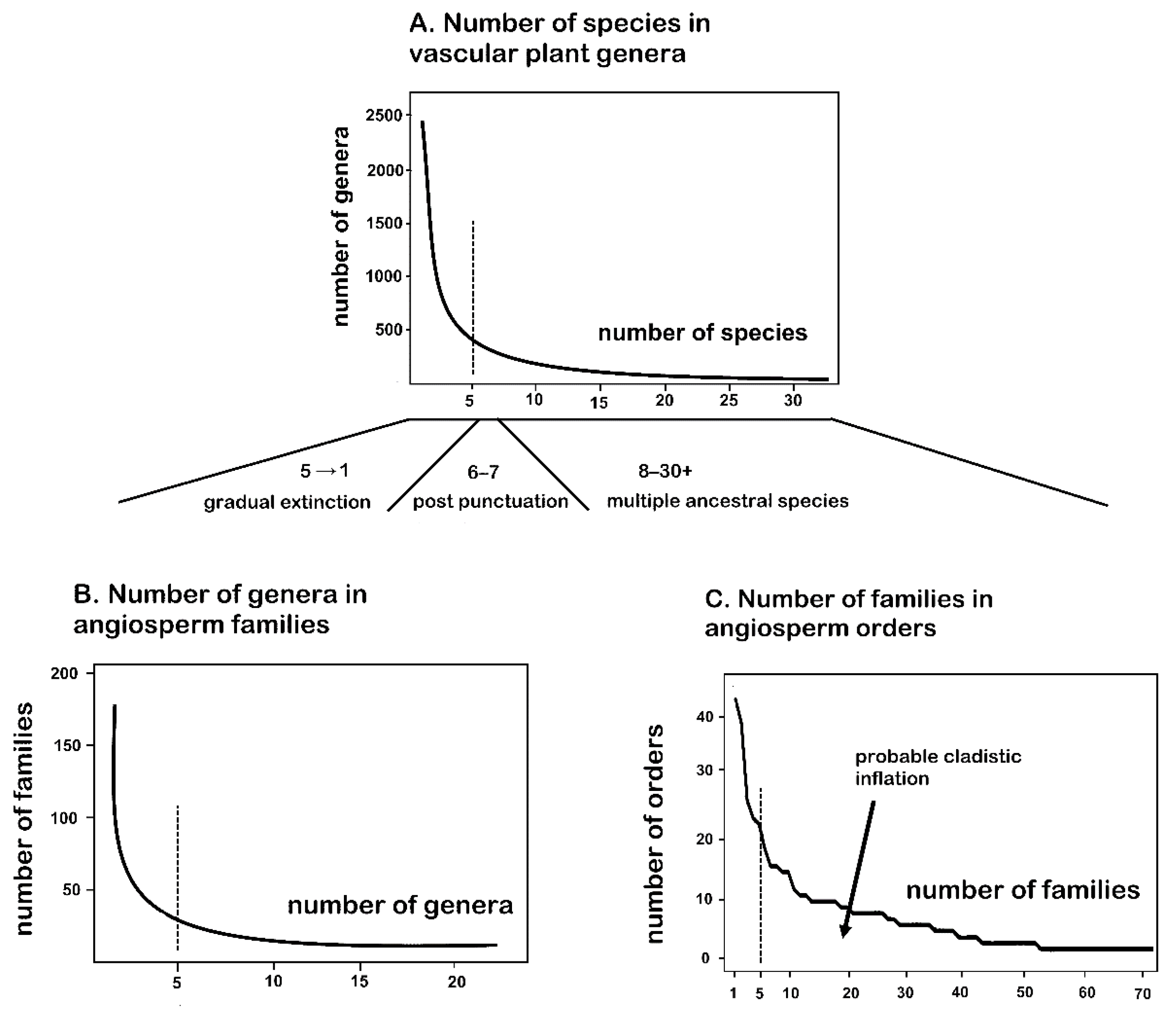
The number of species per genus [16,17], and genera per family [18] have similar hollow-curve graphs (Fig. 1A, B). An additional graph (Fig. 1C) of families per order is here calculated from Web data [19] and shows much the same curve but with thickening of curve beyond five families probably reflecting the increase in number of family synonyms due to recent molecular phylogenetic studies. Given quadrate speciation (generally four immediate descendants from one ancestral species, yielding five total initial species per genus), we can identify the area from five to one on the x axis as gradual extinction from a burst of five. That punctuational burst [20] has been described and justified [20, p. 41]. Given that secondary speciation from descendant species occasionally produced genera of six or seven species, this explains the continued curve, while macrogenera that have not yet been separated into minimally monophyletic groups comprise the low number of genera and families with high numbers of species or genera, respectively. This similarity of the two graphs is fractal, the graphs following a curve with a fractal dimension of about ln5/ln4, or 1.161.
Figure 2 presents an exemplary case for the Rule of Four, that recently evolved microgenera commonly have four immediate descendant species, with up to two secondary descendants possible later. The Pottiaceae tribe Trichostomeae was analyzed for the West Indies [20], an area recently exposed (45 mya) and available for new taxa. Recent land masses are good laboratories for evolution. One branch of Trichostomeae, with Neotricvhostomum crisplum as ancestor, has four descendant genera in that area and contiguous Gulf of Mexico lands. Tainoa is endemic, with three immediate descendants and one secondary speciation. Chiololoma has four descendants, three being endemic and more broadly distributed, and there were two other species in the East Indies that may have originated when these dry island habitats were more or less contiguous during habitat propinquity associated with climate extremes. The other two genera, Weissia and Hymenostomum are nearly worldwide in distribution, originating from populations of N. crispulum elsewhere in the world. The study used the Principle of Mediocrity (AKA Copernican Principle [22] to establish an age of origination of the local taxa at ca. 22 mya. At least regionally, the Rule of Four operated in this group at both genus and species level, while numbers of traits (in Fig. 2) are also mostly four or fewer, not exceeding six. Self-similarity is evident at trait, species, genus, and tribe levels.
Figure 3 shows steps in the inferred timeline of a standard microgenus, a minimally monophyletic group. The caption is fully informative. All the red, blue and green dots are species presently extant and extinct species are not shown. A caulogram is a set of concatenated microgenera connected through their ancestral species by lines indicating timewise origination. Because there are about four traits in all speciation events, and there are no reversals among immediate descendants, all microgenera are statistically well supported through Shannon-Turing sequential Bayesian analysis [23]. Because 20 percent of one ancestral genus generating 80 percent of another descendant genus matches the Pareto ratio, and inasmuch as this process may be found at different taxonomic levels, it is fractal [24] and self-similar (cf. Fig. 1).
1.3. Data on Trait Changes in Species
2. Materials and Methods
Table 3 summarizes the terms and concepts from physics used here to describe analogous processes in evolution. The processes underlying the formulae in evolutionary systematics are more than just likenesses of physical processes, their results are proportional to those of simple mechanics as a kind of Mass Action. Darwinian evolution obeys physical laws [10]. In addition to standard usage in physics, three relevant concepts are introduced here: The initial or punctuational impulse (∫F dt) is the force of the observed initial burst of speciation, the constant of resistance (k) is rate of energy dissipation into the environment, and the Efficiency Ratio measures the useful portion of Work energy.
Results of past study listed above and previously described in detail [1] are here presented as interpreted in timelike and spacelike contexts. Timelike simply means that macroevolutionary processes are conceived as relict groups (extant species and genera) arranged on a caulogram (stem-taxon dendrogram) serially by origination through time, the oldest species at the tree base. Justification for using morphological data in this is: (1) the genera are easily distinguished as microgenera with one ancestral species and one to four immediate descendants all sharing the ancestor’s novel traits (about four, optimally), (2) the progenitors of the microgenera all differ in about the same number of novel traits allowing reasonable connections (caulons, or connecting lines on the caulogram reaching from a species down to the lineage base) between them such that origination of genera is not a new and distinctive operation although the new genera are distinctive qualitatively, (3) the microgenera exhibit gradual extinction as expected, and (4) the new groupings match or are well justified dissections of past accepted taxonomic groups that were originally based on standard omnispection, apprehension of a Gestalt, and generally of native pattern recognition. Most importantly, the use of morphological data in the context of descent with modification (stem-taxon trees) allows detailed and effective analysis with evolutionary mechanics.
Data from Table 1 and Table 2 are analyzed for analogous processes in classical mechanics. The analogues are first defined for taxa and data (Table 3), then used to infer macroevolutionary relationships that reveal processes affecting the relationships of taxa (see Results). Possible constants or universals that may operate as predictive or retrodictive with taxa other than those studied are identified.
The caulograms of the lineages used in this study are then processed to infer what they would look like if viewed at various times in the past. The object is to create a time-ordered set of caulograms as a synchronogram, which would be an image modeling the actual appearance of the caulogram changing over time following its particular evolutionary trajectory. As information, the ordered set of caulograms exists in the present, yet governs a timewise evolutionary process.
The time scales of the lineages used, the moss family Streptotrichaceae [13] and the Pottiaceae tribe Pleuroweisieae [15], have been estimated, using an anchoring fossil and strict morphological clock at 22 my intervals [21] to span 100 my and 88 my, respectively, yielding five and four “slices” evenly spaced through past time, as an informational variant of the Block Universe concept [225,26]. The synchronogram is a spacelike calculation, that is, each past version of the relict-based caulogram is as presented as though viewed in a Common Now. The method of constructing a synchronogram of an ordered set of past caulogram is to reverse the evolution of the present-day caulogram along the lines given by known processes in a single caulogram illustrated in Figure 3 and reflecting the time scales of the order of speciation of the present-day relict genera. As best possible, the actual caulogram at each level of the present-day caulogram is estimated.
3. Results
3.1. Redefinition of Taxa
The point of doing this is that analysis using descent with modification and morphological data has demonstrably higher resolving power than cladistics. This is supported by 250 years of successful independent taxonomic study and the above listed recent advances in systematic methodology. Also, the macroevolutionary diagram (Table 1 and Table 2) are directly based on actual taxa, not nodal intermediates calculated through various methods and data in cluster analysis. Because there is evidence of ancestral-descendant relationships using molecular data (paraphyly-apophyly pairs) that is congruent with morphologically based results [27], morphology is justly freed from being mapped to (constrained to duplicate) molecular cladograms. We start with a redefinition of critical taxonomic ranks or groups some of which are exemplified in past taxonomic study [8]. We can identify four natural taxa. The natural taxa are hierarchical sets of species associated with distinctive macroevolutionary processes. These are the species, genus, lineage and metalineage. Because the last two are not recognized nomenclaturally, standard rank names and concepts are used in practice.
3.1.1. The Species
A species is a group that may include any species concept that works well with the minimally monophyletic genus concept. It is the fundamental unit of macroevolution and classification and of course is distinctive in all the processes of microevolution. The number of new traits established during speciation is about four, which generates by an odds table a two-sigma conduit eliminating uncertainty through space-time, which also individuates the taxon [23]. The species is the natural embodiment of the Hamiltonian concept of momentum as a unit, an observable, in classical mechanics. Speciation is, as a taxonomic measure of macroevolution, a change in a species description, commonly requiring more than two-traits difference to avoid recognizing simple mutations (as one new trait) as evidence of a valid evolutionary group in the context of descent with modification.
3.1.2. The Genus
The genus has the basic control of evolution, and through self-similarity such control may be effective to some extent at all taxonomic ranks (Figs. 1 and 2). The genus, specifically the microgenus of minimal monophyly, is characterized and defined by two criteria: (1) it has one demonstrable extant or otherwise strongly inferable immediate ancestral species, and (2) the novel traits of the ancestral species are all shared with all immediate descendants. The number of important expressed character states changed during speciation is commonly of about four traits (Table 1 and Table 2). The number of descendant species is, significantly, commonly about four, quadratic perhaps due to initial sympatric crowding or later crowding by squeezing of geographic range during glaciations. Extinction reduces over time the number of species in the genus (Fig. 1A) and the ancestral species is most resistant to loss. When molecular paraphyly-apophyly pairs are available in molecular cladistic studies [27] the implied ancestor-descendant relationships support this definition.
Operationally, the microgenus, before onset of extinction, is initially mostly of about five species, one ancestral species and about four descendant species [28]. The ancestral species of a genus is determined by a second-order Markov chain [29], the ancestor identifiable as most similar to an outgroup species and most generalist to the more specialized ingroup species. The microgenus is a complex of long-lasting information mediating macroevolution. In a fashion self-similar to that of the species, the microgenus establishes a two-sigma path through spacetime excluding uncertainty. It uses or is composed of two critical processes embodied in the Pareto Fractal Dimension: (1) The Rule of Four consists of optimally four new traits per speciation event and four immediate descendant species, and there is evidence that taxa at higher ranks also are quadratic in nature, and that in physics it is a meta-law of nature [30,31], while, of course, there are four primary nitrogenous bases in DNA optimally so through information theory and pairing constraints [14 p. 128,32]. (2) The Evolutionary Fractal Dimension operates in which a descendant of one genus generates four of its own descendants sharing the same novel traits of itself. In such manner the new genus then has five species sharing the same traits. Thus, we have the Pareto ratio where 20% of the first genus generates 80% of the second genus, involving a fractal dimension of ln5 / ln4, or 1.161 [29]. The hollow curves of Figure 1 are of the form, equivalent to the Pareto Fractal Dimension:
This expression is a power-law decay and is modeled by Figure 3 in which one species of one genus gives rise to four species of a second genus, that second genus having all new traits of its immediate ancestor. Genera larger than five species may originate after the initial punctuational event by secondary speciation of descendant species. Unstudied larger groups are called mesogenera and may include than one ancestral species. The equation for the Pareto Fractal Dimension (Equ.1) is doubtless a result of underlying variables [33] associated with fundamental constraints on speciation; this paper follows the distinction between underlying laws and equations and the theory of the mechanisms applying these laws [34].
The denominator ln5/ln4 in Equation 1 is the shape of the curve reflecting Pareto evolutionary change, while the numerator in power laws ]35–37] sets the height of the curve relative to the y-axis, which reflects the number of items (species richness) involved. The numerator of 16 moves the curve so that the number on the x-axis (number of genera) tells you the number on the y-axis correct for the actual counted number of species per genus. That numerator is a scaling factor [38,39] that fits the actual curve best and represents the resistance (possibly by crowding) to adding new species (species per genus) as the genus grows. The number is sufficiently large that even a small environmental shift results in a large evolutionary pressure. The numerator is the proportionality constant λ in the inverse power function f(x) = λx–α and α is the fractal dimension ln5/ln4. That dimension is a taxonomic crowding factor related to the Pareto ratio. The numerator 16 represents a fractal square of the Rule of Four for immediate descendants where secondary speciation by usually limited to two immediate descendants and reflects a large selective pressure on the first one or two descendant species. Adding two more descendants to the genus totals seven species as maximal richness as empirically evidenced and explained below as a result of a Constant of Resistance.
3.1.3. The Lineage
All taxa of rank larger than the genus may be modeled as descent with modification on a stem-taxon tree, a caulogram. Ancestral taxa of microgenera are connected along lines leading to the base of the caulogram, each line is a caulon consisting of an ordered series of ancestors. Numbers of trait changes on speciation are much the same as internally in a genus, about four. When double or more traits separate microgenera (ancestor to ancestor), an extinct genus may be inferred. All taxa above genus that may be arranged as a caulogram and subsumed under the natural taxon “lineage” although for historical reasons lineage has no formal nomenclatural standing. A lineage is a natural taxon because, like species, genus and metalineage, it is associated with distinctive evolutionary processes and is not simply a hierarchically nested self-similar set of the species as are tribe, family, order, and so on. Lineages of Streptotrichaceae, Pleuroweisieae, and other bryophyte taxa are diagramed and discussed in previous papers [8]. The former two have been somewhat refined and are arranged as spreadsheets in Table 1 and Table 2.
3.1.4. The Metalineage
Aside from species and genera, higher taxonomic ranks are here all address by the taxon-like constructs of a timelike lineage or a spacelike metalineage. Timelike means a process sequential in time. Spacelike means simultaneous or coetaneous, with all information immediately functional [7], controlling the physical expression. The timelike lineage is modeled as a caulogram (Table 1), which is a branching evolutionary connection between the progenitors of microgenera as ordered by inference through time. This is the unitary lineage of branching lines of sequential descent on a stem-taxon tree and is featured in recent major publications [8]. A strict morphological clock for the timelike series has been employed with caulograms [28]. Although not conceived as ticking by neutral mutation accumulation, a morphological clock matches the breadth of time of the “modern flora” reaching back to the Upper Cretaceous, matches a fossil anchor, and the relevant caulograms show only even, gradual change in accumulated numbers of novel traits.
The spacelike metalineage is a new concept that acts as a taxon. It summarizes the substance and history of timelike data. A metalineage is modeled as a synchronogram, being an n-tuple or ordered set of caulograms, a superset of data about the present-day lineage. (A tuple is like a row in a spreadsheet.) The subject of this paper is the distinction of species, genera, lineages and metalineages as measurable, scientifically real structured information lasting millions of years in the genetics of groups of organisms and influencing the course of evolution.
The synchronogram of a metalineage consists of series of caulograms of the same lineage each in a form inferred to have existed at some particular time in the past. Four caulograms in the set are sufficient to ensure a two-sigma exclusion of uncertainty because they are the equivalent of the number of species in the genus. The future of the present-day lineage, given that no information is available except that of the past, may be predicted only to the extent of extinction of present-day taxa. while prediction of potential new taxa must be calculated with other techniques, if possible.
Figure 4.
Two metalineages, the related moss taxa Streptotrichaceae and Pottiaceae tribe Pleuroweisieae. These are imaged as synchronograms ordering calculated past caulograms as tuples. There is no timelike vector as all caulograms, as inferred samples, are considered to operate as information at once. The caulogram farthest to the right in each metalineage is that of the present-day composition of the lineage, essentially the past 22 my. Dots are genera, solid are extant genera, hollow are extinct. Numbers are of numbers of descendants estimated as extant at the time, the branch leading to next genus is an additional descendant. Double-headed arrows indicate that these are calculations free of the arrow of time, i.e., the information is extant, here treated as a unitary living structure.
Figure 4.
Two metalineages, the related moss taxa Streptotrichaceae and Pottiaceae tribe Pleuroweisieae. These are imaged as synchronograms ordering calculated past caulograms as tuples. There is no timelike vector as all caulograms, as inferred samples, are considered to operate as information at once. The caulogram farthest to the right in each metalineage is that of the present-day composition of the lineage, essentially the past 22 my. Dots are genera, solid are extant genera, hollow are extinct. Numbers are of numbers of descendants estimated as extant at the time, the branch leading to next genus is an additional descendant. Double-headed arrows indicate that these are calculations free of the arrow of time, i.e., the information is extant, here treated as a unitary living structure.
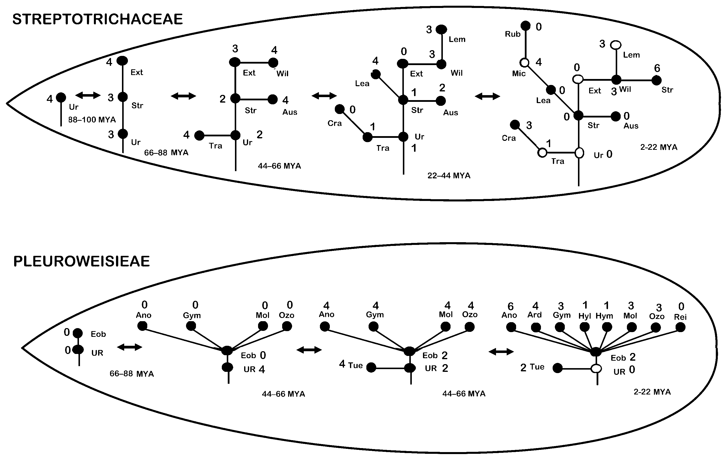
The calculations for generating a metalineage are made from present-day relicts (extant species and genera) modified by expectations of past change taking into account the common evolutionary processes (Fig. 2 and 3) established by the Rule of Four and Pareto Fractal Dimension.
The two metalineages (Fig. 4) extend 88–100 my. The five caulogram slices for Streptotrichaceae image are calculated caulograms that were extant in the earlier and the later Upper Cretaceous, the Paleocene-Eocene boundary, the late Eocene and Oligocene, and the Miocene up to the Pleistocene. The synchronogram for the Pleuroweisieae is ordered likewise this lineage is apparently (by calculation) absent in the earlier Upper Cretaceous. This tribal lineage is apparently somewhat less ancient than the Streptotrichaceae. The synchronograms are similar to the evolutionary time-form lattice of Gingerich [40], except that the time-form lattice is scaled by generation time, while the synchronogram is scaled by a 22 my morphological clock. Gingerich, also, found for Cenozoic mammals rapid, punctuational filling of available niches followed by long-term stabilizing selection.
Twenty-two million years have been proposed as time interval for the strict morphological cloak for these groups [21]. The numbers of species and genera in the four or five time slices used (Fig. 4) indicate no great change across time in numbers of taxa for both groups since inception in the Late Cretaceous. The numbers of species for each slice of time in the caulograms are an indication of the impetus (momentum or mass times velocity). The numbers of species for Streptotrichaceae time slices, from origin through present are 5, 13, 25, 24 and 27. Those for Pleuroweisieae are 2, 20, 31 and 35. Apparently, after origination, the numbers of species in each of the two lineages extant over time are not much different across time. This may be attributable to saturation of the available habitats given phyletic constraint on the available adaptations of that taxonomic lineage.
In ecological terms, if the species is equivalent to its niche, then the numbers measure the niche availability where evolutionary change deals with changing environment. If the spacetime path of each species is a branching “fiber” then the “rope” of the metalineage is remarkably even in thickness. Its long-lasting individuation is due to a massive exclusion of uncertainty on a broad front.
The changes in the species composition given origination and extinction are rather balanced possibly reflecting the gradual diminution of global temperature and other environmental changes through the Miocene and Pliocene since the Paleocene-Eocene Thermal Maximum about 56 mya. In addition, the Rule of Four provides constraint on generation of descendant species. One may assume, given that each species has long persisted under the same habitat conditions, that the average numbers of traits per species, 4.3 for Streptotrichaceae and 4.54 for Pleuroweisieae [15] are much the same in the timewise slices as in the present. The present evolutionary Force values for each lineage are also similar, 710 for STR and 753 for PLE. Given that the habitats of the two lineages are rather different13], there may be an optimal or maximal size in numbers of species globally, reinforced through competition associated with crowding during glaciation and other habitat consolidations.
3.2. Formulae for taxon-Based Evolutionary Processes
Analysis of the data is predicated in successful use of physics and statistical methods in other fields and with other taxa [41,42,43,44,45,46,47,48,49]. These works, on the other hand, are usually focused on microevolution, e.g. evolution in and between populations not macroevolution, and are commonly statistical not deterministic (as is mostly the present paper).
Classical mechanics uses position and momentum for many basic calculations, the standard six dimensions being three for position and three for momentum. Position, in the context of taxonomy, is where an individual or group is placed somewhere in taxonomic space, in particular on an evolutionary tree. Knowing a species’ immediate ancestor establishes position immediately.
Velocity and momentum are first and second differentials of position, easily applicable when acceleration (change in velocity) is constant, but which it is not the case in evolution. If an arithmetic progression grows by a constant rate, the total grows according to the square of the number of steps, but trait changes along a caulon are not constant in number. The work-around is to consider instantaneous acceleration as the plus or minus change in velocity of a species in respect to its immediate ancestor, with the historical acceleration being the sum of all current accelerations on the caulon for any one species.
The formulae for evolutionary mechanics are based on those of classical mechanics and prove informative. Evolutionary mass is simply a species, e.g. 1 sp., and changes analytic focus from the motion (displacement) of a population to the motion of a lineage. Taxonomically an evolutionary species is a species description, which changes somewhat during speciation.
Evolutionary time tevol; is a speciation event, e.g. 1 sp.ev., which may involve ca. four species originating about the same time from one joint ancestor, but applies to only one of them. Time may also be measured in larger units for purposes of comparison, such as distance per lineage when comparing lineages.
Evolutionary distance devol is simply the number of traits changed in each speciation event added up from the position of a species on a caulogram down to the base of the caulogram.
Distance is an important measure by itself and is a justifiable measure of comparative resilience through time as historical sustainability.
Velocity is a measure of motion, and momentum as mass times velocity is a measure of persistence. Current or instantaneous evolutionary velocity vevol is the single number of changed traits ( ) divided by the time as one speciation event sp.ev.
Current velocity measures the present speed of change for one species in that caulon as a single increase of traits in one speciation event, and it also establishes a two-sigma conduit excluding uncertainty through spacetime for that one new species, individuating it. Velocity of lineages has been modeled for cladograms [43].
Cumulative velocity vcumevol is the summed numbers of trait changes along a caulon divided by the number N of speciation events sp.ev., here Nsp.ev. :
Cumulative velocity is a scalar measure of the almost steady pace of change of position of that species since the origin of the lineage.
Momentum p classically is p = mv, or mass times velocity, a vector. Current momentum is the directional force of the lineage at one speciation event. If mass is 1 species, then:
pevol= vevol
This is the same as velocity given that m = 1 (that is, one species). The difference is that the velocity is the rate of change while momentum is the force of inertia as an impact. Momentum increases linearly with speed (v). The current momentum is a measure of the amount of force needed to stop that one species in the lineage from any evolutionary change (turn it to stasis). Also, the average of all current momenta is a measure of the average force needed to stop into stasis any one species in the lineage, while the sum of all current velocities is the force needed to stop a lineage by stopping all species at once.
Cumulative momentum is a vector measure given the average directional strength of the lineage over its time of existence (a bar or arrow above the variable means it is a vector):
where is total distance divided by total speciation events leading to the species and may be termed historical inertia for that one species. This is the historical legacy or weight of evolution for that lineage ending in that one species. Summing cumulative momentum gives the directional weight of evolution for the lineage. A high cumulative momentum implies a deep macroevolutionary trend.
Force is mass times acceleration (F = ma) or deceleration if a is negative. It may be interpretable as increasing or decreasing resistance to environmental change. Acceleration is the difference, positive or negative, between the number of novel traits of one species (its rate) from that of its immediate ancestor. Cumulative acceleration is the sum of rate changes for one species (one mass) in a caulon divided by the number of speciation events. If the acceleration is not constant, as in evolutionary series, then the average rate (velocity at end minus velocity at beginning) is used such that a = average velocity / number of speciation events. Total Force for a mass of 2 or more species is then the total mass times their average acceleration. For example, if the ancestor’s initial rate (vi) is 1 trait per event, and the current species rate (vc) is 5 traits per event, the acceleration would be 5 − 1 = 4. The Force for that current species would be +4.
Force may be measured in other units of time, not just speciation events. Force using acceleration per speciation event is used for comparing internal processes of a lineage, but one may use time as per lineage for comparing lineages. For instance, in Zander [15] Force was measured in time units of lineage events (“lineageation”), where acceleration is the difference between final velocity (∑trait changes) and initial velocity (zero) divided by time (1 lineage). Of course, a species only exists since its origination in the lineage, not back to the origin of the lineage, but what is accelerated as mass during each speciation event is the species description, of about 45 characters in the present study borne along by a succession of trait changes. This is like the final speed of the final stage of a multistage rocket. As the description lasts fairly intact with each speciation event (shared description is why it is a lineage), acceleration of any one species per lineage (as time) is the sum of all trait changes in the caulon down to the lineage base (minus zero trait changes lineage start), divided by time (1 lineage).
Total work is the force needed to displace an object by a given distance. In this case, the sum of one species’ average acceleration times current velocity (distance). Work is equal to the change in kinetic energy except when there is a push-back against Work from environmental resistance.
The TAU is here a new measure defined here as the Work (F × d) done by one unit of selective force over a distance of one trait change one unit of time (a speciation event). This is equivalent to KE () of 1 species (m = 1) changing at a rate of one trait per speciation event (v =1), given the fundamental dimension of traits2/events2. The TAU is the evolutionary analogue of the joule.
Kinetic energy (KE) increases exponentially with speed (v2), and is given by the formula:
Work and kinetic energy are both measures of energy but arrived at in different ways. Kinetic energy is the ideal energy of evolution without resistance from environmental pressures.
Potential energy (PE) is tension to diversify, or force of selection times the unrealized change in traits.
PE = Selection Force (F) × Unrealized Change (Δd)
It is the as yet unrealized portion (PE) of the initial adaptive potential of 16 (numerator of Equ. 1) representing a potential 16 species having total energy (KE +PE). It is the initial evolutionary capital. Total energy (KE + PE) is when the genus is young and not yet undergoing resistance. The difference between total energy and KE is the draining of energy where PE is dissipated by being converted to KE. The Force decays by the power law function as genus grows in number. The PE implied by the numerator 16 in Equation 1 reflects real data that includes massive genera, and as will be explained below is probably better replaced (for Fig. 1) by 4 as PE for initial burst of four descendant species.
3.3. Analysis of Spreadsheet Data
Table 4 and Table 5 summarize numbers and rates of change in two lineages, Streptotrichaceae (STR) and Pottiaceae tribe Pleuroweisieae (PLE). These are here interpreted as to their evolutionary significance given processes similar to those of classical mechanics.
Distance (ToTrCa) STR and PLE have about the same number of traits total 710 and 753, respectively, averaging about the same number of total caulon trait changes per species, 21.5 and 20.9. This is their evolutionary distance in total numbers of trait changes.
Time (ToEvSp) is here measured by successive speciation events, with STR having 161 sp.ev. averaging 4.88 per caulon, and PLE with 135 sp.ev. averaging 3.75 per caulon. STR has a longer time of evolutionary existence than PLE, as shown by number of numbered columns in Table 1 and Table 2.
Current or instantaneous velocity (InVel) is restricted to the number of traits changed in the last speciation event for one species, that is v = d/t for just one speciation event. STR has 137, averaging 4.15, and PLE 123 averaging 3.42. Thus, STR has a more robust adaptive response than PLE.
Cumulative velocity (CuVel) is the total velocity divided by total speciation events. It is the average speed of the lineage’s change, or historical legacy or evolutionary weight. Comparing current velocity with overall velocity shows whether there is a slowing or increase in evolutionary velocity for that species. All the species travel at somewhat different rates yet the lineage moves as a unit being adaptively coherent on account of their shared traits. For STR, this measure is 143.5 averaging 4.35, for PLE it is 204.3 averaging 5.67. Comparing cumulative and current velocities indicates that STR (137:143.5) is slowing the rate of adaptation, while PLE (123:204.3) is slowing even more so. A common cumulative velocity is the result of processes holding a lineage together.
Current or instantaneous acceleration (AccIns) is simply the increase or decrease in numbers of new traits from the one immediate ancestor. Adding current acceleration for all species (negative and positive rate changes in the spreadsheet column) for STR yields −1 averaging −0.03, and for PLE gives −30 averaging −0.83. Here PLE shows a major lineage-wide (and long) decrease in adaptive power.
Force when used to compare internal lineage processes is mass (species) times current acceleration for one species, essentially the same as current acceleration (AccIns) for any one species. The average current acceleration is used for force of multiple species. Force is equivalent to selection pressure. When comparing lineages, Force is calculated with acceleration as change in velocity from beginning of lineage (zero) to each species (∑trait changes). The total Force for lineages is simply the sum of all trait changes leading to each species (ToTrCa), which provides comparative Force values of 710 averaging 21.52 for STR and 753 averaging 20.92 for PLE. Evolutionary Force is similar for the two lineages but distributed differently through the lineage and through time, see comparative values of velocity, acceleration and Work.
Total acceleration of genera (ToAcGe) summarizes the change in rate of trait changes for all species in a genus. For STR the total is −2, averaging 0, while for PLE the total is −22 averaging −2. Again, STR demonstrates higher rate or at least force of adaptation, and particular genera in these lineages may be signaled out as well adapted in STR (Crassileptodontium and Austroleptodontium), while some in PLE are apparently very weakly adapted to current conditions (Anoectangium, Gymnostomum, Ozobryum) although some species in each are much better adapted than others.
Work is Force times total distance as a measure of evolutionary power overcoming entropy and ensuring homeostasis, as measured in Taxonomic Action Units (TAU). Work for STR is −326.0 averaging −9.9, while for PLE it is −610.0 averaging −16.9. The negative values is the energy cost of the environment and indicate that work is energy dissipated by environmental friction (resistance). Clearly STR is more efficient in operating against environmental resistance.
Kinetic energy is viewed as acting force of evolution. For STR the values are 312.5 averaging 9.5, and for PLE the values are 268.5 averaging 7.5. Comparing total Work and kinetic energy values (Table 3 and Table 4) gives an idea of the resistance of the environment to the evolutionary force of the lineage. For Streptotrichaeceae, Work value is −9.9 and KE is 9.5; there is a net energy of −0.4. In Pleuroweisieae, Work value is −16.9 and KE is 7.5; there is a net energy 0f =−9.4. There is an energy deficit for both lineages, but the amounts differ greatly. See discussion of Efficiency Ratio below.
Potential energy is the difference between KE actually realized, and total possible energy (E), as measured in Taxonomic Action Units (TAU). For example, if a species is currently changing at six traits per event (v = 6), pressure is steady with Force = 1, it is almost at its adaptive peak, thus the adaptive gap (Δd) = 1. By Equation 7, KE = 18, and PE = 1 × 1, or 1. Total energy (PE + KE = E) = 19. If the Force is higher, PE is higher, and so is E. If an ancestral species has 2 changed traits and its immediate descendant changed 6 traits, then acceleration is 6 − 2= 4; mass = 1; and Force is then 1 × 4 = 4. In this latter case, the environment provided a Force of 4 to the descendant to make it evolve three times faster than its ancestor.
Evaluations of the PE of individual species are easily made from Table 1 and Table 2, where high PE implies high adaptive tension with environmental Force restricted by high resistance or drag (k). The PE provides the initial impulse for speciation by the environment, and immediately becomes KE, which decays at the rate of 1/x1.161, the inverse function for the Pareto Fractal Dimension. The actual data (Table 1 and Table 2) reflect the expectation that the first 1–2 descendant species are powered by initial strong KE, while the next 3–6 do not accelerate and are sustained by residual KE (KE decays while k remains constant), while at species 7 the cumulative Work of friction (∑Wk) equals the initial impulse (J), resulting in net energy of zero. This is the evolutionary mechanics of the origination of species.
3.3.1. Punctuational Impulse
Punctuational Impulse is the initial force of 4 that generates an initial four species per speciation event. This force is in terms of Taxonomic Action Units (TAU) which is one species generating one trait change versus environmental resistance. After the punctuational burst, PE is converted to KE by Equation 7. Basically, for an expected punctuational event generating four new species, PE has Force = 4, which goes to zero upon speciation of four descendants. The PE value is then doubled through the KE formula. The energy calculation is:
The PE Force of 4, lineage-wide, banks 8 units of KE into the system, and apparently entirely and finally countered by a diminution of KE by total extinction over up to 100 my for the lineages here studied but continues as important for recently evolved genera. J is Force times time (one speciation event). It is zero for all genera with eight or more species due to dissipation during initial and secondary rounds of speciation, resulting in punctuational equilibrium, i.e. a genus stable in numbers of species. The impulse is the source of potential energy. After speciation, the KE is 8, being the momentum of four new species. This explains why secondary speciation (immediate descendant species having descendant species of their own) are limited generally to 7. Genera that stop at only 4 immediate descendants (5 total species) would have a high friction value of 2.0, which would be a cumulative measure of environmental constraint. The number 16 in Equation 1 represents the environmental demand (the potential field PEmax) while the number 7 here is the actual displacement (distance or efficiency limit). At 7 species the Work of friction (k × d) cannot reach the theoretic capacity of 8.
3.3.2. Constant of Resistance
The details of why the Rule of Four and Pareto Fractal Dimension limit genera initially to only four immediate descendants and only two secondary descendants involve calculation of resistance (k) to drainage of energy by extinction, niche competition, and genetic stasis, here equated with physical friction. The stalling at around 7 total species of generation of numbers of descendants in a genus follows:
The Work-Energy Theorem of Equation 10 is also written as Wk = ΔKE. The initial KE from the 4-species (the numerator) burst is 8 Taxonomic Action Units (TAUs) or Force × d) following Equation 10. This is selective pressure. Distance in these calculations is numbers of species, where a burst is 4 species and a stall is 7 species. Total species possible is 7, determined empirically as the limit in numbers of all species in a genus. As mass is one for each species, and 8 divided by 7 is 1.14, which is the value k of evolutionary friction or the Constant of Resistance for these lineages. This is the drain of evolutionary energy taken away by the environment. At species number 7, cumulative friction is 1.14 × 7, or 7.98, exhausting the evolutionary impulse of 8 (Fig. 5). The numerator of the inverse function in Equation 1 of 16 is a feature of actual data for species per genus including many genera of many more than 7 species, and reflects large numbers of species at x = 1, yet graphs based on actual microgenera (Zander Force 2025, there Figure 2 and Figure 3) show cut off for STR of 7 and 8 for species/genus and traits/species, respectively; and cut off likewise at 7 and 8 for PLE.
Quite probably the proper inverse function formula for the Pareto Fractal Dimension curve is f(x) = 4/x1.161 as the Fundamental Unit of Diversification. The graphs of Fig. 1 that apparently are generated by f(x) = 16/x1.161 are a secondary expansion of the Rule of Four . The numerator of 4 is the selection pressure of the environment. One would expect that different environments have different friction values, but the rather different habitats of the two lineages studied here seem to have the same values for k, which are possibly constant across 100 my. In sum, adaptive tension of 4 is drained over time by the constant of evolutionary friction of 1.14 TAUs per species.
The Energy Balance Equation for species evolution is KE of 8 TAU from a punctuational burst of 4 minus distance (number of descendant species in a genusation event) times the constant of resistance (k or friction):
KEcurrent = KEinitial − (k × d)
Substituting the formula for KE ():
Solving for v (evolutionary velocity):
Given that the known maximum for numbers of species in a microgenus is 7, the velocity for a series of species generated closely in a burst by an ancestor is: 1 species, 3.7, 3 species 3.0, 5 species 2.1, 7 species 0.2. Thus, at 6 descendant species, the energy from selection pressure to generate additional species begins to peter-out, while 7 descendant species (8 species total) in a genus is not supported. Figure 5 illustrates the curve of evolutionary force, which is nearly identical to the inverse power function of the Pareto Fractal Dimension. Figure 6 illustrates the evolutionary velocity decline, a curve that well matches Heaps Law [39]. The velocity of evolution is therefore a finite and measurable resource. A second impulse of environmental selection generates a new genus which evolves in number of species in the same manner. The stalling of species generation is a function of the square root of declining energy.
The graph of Figure 6 shows exhaustion of energy at 7.2 species. The y-axis is the evolutionary speed of about 3.7 near the origination of the first descendant species. The area under the curve is the total displacement or divergence of the genus through the trait landscape:
The area under the curve is 18.7 trait units, meaning that a genus of 7 species has an accumulated 18.7 units of morphological divergence from the immediate ancestral species by the time the seventh species originated. The genus is 7 species in length but 18.7 traits in width, the latter measures the disparity or variability in the genus. This measures in terms of TAUs the evolution of these lineages as a zero-sum game. A Rule of Eight describing no descendants possible for total species in a genus is then a corollary of the Rule of Four for descendant origination. Thus for a punctuational impulse of 8 TAUs, and an efficiency of 1.14 TAUs lost per species event, the output is 7 species total with a morphological ceiling of about 20 TAUs.
The square root of two (1.14) determines the velocity (rate of change in traits) from the KE: v = , such that velocity matches KE. If initial impulse J is 8 TAUs, the velocity = 4. Inasmuch as STR and PLE have same point of stalling of species generation, the Constant of Resistance (friction) of 1.14 implies that the square root of two is a universal law of taxonomic decay.
3.3.3. Stalling
In the present model, an environmental force of 4 providing an initial KE impulse of 8 (one-half of 4 squared, Equation 10) in kinetic energy is countered by friction (k)from the environment. When friction and potential energy (environmental driving force for change) become equal, evolution goes to zero: KE −Wok of friction (1.14 × d) = 0, and E becomes 0. At zero, velocity (number of new traits) is zero. The exhaustion of total energy is more probable when acceleration is zero (that is, number of immediate ancestral state changes are same as descendant state changes). The species is then in stasis, moving through time on the momentum of its maintained velocity (where the number of new traits is the same as that of its ancestor) but lacking KE to resist negative changes in the environment. For the formula f(x) = 4/x1.161, at Species 1, E = 8.0 (high vitality); at Species = 4, E = 8.0 − (1.14 × 4) = 3.44 (stable but slowing), at Species 7, E = 8.0 − (1.14 × 7) = 0.02 (brink of energy expended). There is no kinetic energy left for species origination (Fig. 6) and the genus stalls in number of species. The genus then undergoes gradual extinction. The value 1.14 (square toot of two) is k the Constant of Resistance which may prove to be universal.
3.3.4. The Efficiency Ratio
Efficiency Ratio (η) is a measure of the percent of total energy input (Work) converted to useful output. It is possibly the best measure for comparing the evolutionary mechanics of lineages. The formula uses the absolute value of energetic Work |W|:
The efficiency ratio for STR is, before correction (see below) 104.2%, while that for Pleuroweisieae is 44.38%. The Streptotrichaeceae is highly efficient in using its evolutionary power, but the Pleuroweisieae has much of its energy devoted to genetic load (deleterious mutations), environmental buffering (cost of retaining stasis in face of hostile environment), or adaptive constraints (difficulty adapting given form and function), thus, in all, dissipated as “evolutionary entropy.” Forces theoretically involved in balancing speciation rate versus extinction rate has been detailed for cladograms [17].
In the present model, mass is treated as one species, and time as successive speciation events. As velocity is the change in traits per change in species events, squaring this gives change squared over time squared, or KE units. Work is acceleration times distance or change in traits per speciation events squared, times distance, which comprises the same units as KE, or (trait changes)2/(distance)2. The evolutionary pressures for STR expressed a total energy change 312.5 TAUs (sp.2/sp.ev.2) averaging −9.5, and actual divergence average was −326.0 TAUs averaging −9.9 nearly the same, which may be due to stabilizing selection or phyletic constraints. Greater energy in the result (divergence) than apparently available (Work), that is, the difference between −326.0 and −312.5 TAU, or 13.5, implies additional energy from elsewhere. This discrepancy is actually due to the fact that there is no acceleration for the first taxon at the base of the caulogram but there is inferable velocity (distance as number of new traits divided by time or one speciation event). Thus, subtracting the absolute value 16 for Work for IEG1, reduces the total Work to −310.0, averaging −9.4 TAU. The corrected efficiency ration for STR is 100.8%, meaning that essentially all Work is accounted for by available KE for STR.
The evolutionary pressures for PLE in Table 2 are a total energy change of 16.9 TAUs, compared to actual divergence of 7.5 TAUs, an efficiency ratio of only 44.38%, imply that 9.4 units of energy are absorbed or dissipated by this lineage rather than used in adaptive trait change. Correcting the high Work value of 64 TAU for no acceleration in the one IEG at the base of the caulogram by subtracting 64 from the absolute value of total Work, 610.0, or −546.0, averaging −15.2, the actual efficiency ratio for PLE is 49,5%. (268.5/546.0 × 100). The PLE system has high impedance, with half the energy lost to environmental friction.
Other metrics for evolutionary distance use phenotypic units like centimeters, e.g. haldanes, using standard deviation per generation (e.g. [40]), or darwins, this being e-fold change in a trait per million years. The present equivalence of species, speciation events and character-state change with physical units of mass, time and distance provides a new, rich perspective on macroevolution.
4. Discussion
Physics is a broad subject but the basics applicable to taxonomy are not esoteric. An excellent primer for the classical mechanics used in the present paper is the introductory book by S. Carroll [50], while other aides suitable for taxonomists are available. The present study recasts the taxa of evolutionary systematics in terms of physics, particularly position and displacement that are equivalent to place on a caulogram, and rate and change in rate of character state changes. Macroevolutionary processes and possible universals may be theorized through analysis of expressed traits along the lines of descent with modification. The term evolutionary mechanics has been used [51] for phylogenetic analysis of the origination of proteomes, but without direct parallelism with classical mechanics.
There are four hierarchical taxonomic levels here identifiable as well-supported evolutionary groupings: the species, the microgenus, the timelike lineage (caulogram) and the spacelike metalineage (synchronogram or tuple of timewise caulograms). These groups are of evolutionary substance initiated and governed by clear and effective processes through time that may at least in part be evaluated with principles of physics. They are useful in prediction of sustainability and evolutionary force that contributes to survival at the ecosystem level, that is, Darwinian selection among lineages that maximizes an orderly digestion of Gibbs free energy through niche saturation and trait redundancy. The caulograms interpreted with the Rule of Four and the Pareto Fractal Dimension extend the ability to predict and retrodict the evolutionary trajectories of lineages in general, while such helps gauge the extent of a synchronogram, that is, when and where it may “pinch off” in retrodiction of its origin and prediction of its possible demise.
Taxonomic information may be used to do rather complex investigations of evolutionary processes. For example, evolution is uniform or stable when velocity, as distance per time, or species per speciation events, is constant, and acceleration is thus zero. If evolution is constant, maintaining its current rate of change (gradual additions and extinctions of traits and species) the environment is stable or at least matching change rates. Primary speciation may be viewed as bursts of genus-level isomorphism in shared immediate-ancestral traits. Secondary speciation cleans up excess kinetic energy. Redundancy of expressed traits apparently is a major factor in sustainability.
The complexity principle [52,53] of the conservation of evolutionary processes across scale is suggested here as implied by similar inverse power curves for species per genus and genera per family (Fig. 1A, B). This would imply that the two-sigma exclusion of uncertainty, the Rule of Four and the Pareto Fractal Dimension operate at all taxonomic ranks. Further work is needed for confirmation of this replication as part of the fractal complexity of taxa ]54]. Self-similarity would be parsimonious of energy in the development of these powerful controlling mechanisms.
A metalineage is not a causal series, but an ordered series of models of what the caulogram might look like at various times in the past. There is no arrow of time as all this information exists in the present and is actionable information about at least sections of a single timewise living structure. When a basal species in a caulogram cannot be connected to an earlier species by a few novel traits, then the metalineage is terminated with the expectation that information on earlier taxa is lost due to environmental factors, creating a process-based informational gap. Doubtless earlier metalineages are concatenated in series (like gregarines), but exact connections are unknown. This may be compared with an attempt to characterize mathematically a cladogram as an informationally based living tree of life [42], comprised by multi-fractal structure of biological lineages. Results of that study are theoretical, however, without extensive exemplification as in the present paper, but the work has a similar foundation in physics.
The number of possible caulograms comprising a metalineage is limited by the number of relict species available to the observer because information is unitary as bits and is precisely ordered. As an egregore—an influential collective thought-form—a metalineage modifies or educates its observer but only to the extent that the observer recognizes the information. A metalineage is the largest living structure, with evolution propelled by central attributes of life: homeostasis, responsiveness, self-corrigibility, entropy-generation, adaptivity, having ecologically integrated parts, and robust sustainability of form and function. One may think that, without the balance of homogenizing and differentiating features associated with microevolution, a constantly fanning lineage (except for possible horizontal gene transfer) is on initial consideration hardly a functional adaptable unit, but small trait differences between ancestors and descendants plus the multiple million-year survival between speciation events of this long-lived living structure indicate otherwise. Perhaps the redundancy of ancestral traits [55] associated with Pareto-ratioed genusation events provides the needed genetic reserve?
The synchronogram, given the extra information provided, is far more than just an interpretation of that one caulogram. The tuple entries of a metalineage are equivalent to the description of a taxon, with four or five time slices as “traits.” The caulograms in the synchronogram tuple are all of the same taxon (tribe or family as a lineage), thus have the proper formal nomenclature. If the original present-day caulogram has four or more time levels (series on a caulon line), then it is well individuated with two-sigma exclusion of uncertainty. The number of levels of information depth is equivalent to a set of characters, each of one informational bit. Following an odds table [21, p. 17], one bit excludes 0.67 of uncertainty (one sigma), four 0.94 (ca. two sigma), nine 0.998 (three sigma).
This study claims it is high-resolution phylogenetics because analysis by descent with modification on stem-taxon trees independently using morphology and molecular data (Zander integrability) demonstrably yields more and stronger inferences on evolutionary processes than present-day cladistics using any data or analytic method. The most relevant difference between analysis by decent with modification (structural monophyly) and by shared ancestry (cladistics) is that dichotomously branching cladograms of the latter restrict Force values to 2 artificially due to cluster analysis techniques, while caulograms flexibly allow empirically based (by tetrachotomies in recent genera) Force values of 4. This is confirmed by demonstrable constraints of macroevolution: the Rule of Four with isomorphism of novel ancestral traits, the Pareto Fractal Dimension, and in physics the meta-law of nature [31,32].
4.1. New to Science
Certain results should be particularly emphasized as new to science: Discerning analogues in evolutionary taxonomy of processes in classical mechanics allows analysis of heretofore unrecognized physical relationships between taxa. The Rule of Four, Pareto Fractal Dimension, and minimally monophyletic groups are quantifiable and integrate well in complex formulae. The hollow curves figuring in Willis’ Age and Area study [56] inform the methods of evolutionary mechanics. There are four natural taxa defined as part of a mathematically coherent grand organizational contribution to ecosystem resilience, with the metalineage introduced as new. Speciation, secondary speciation, stasis and extinction are common orderly processes that are measurable and predictable as involving energy exchanges. There is a physical exchange rate between the number of species in a genus and the number of traits in that genus. A genus of 7 species must have about 20 traits given an impulse Force of 4. Punctuational (ca. 22 my) speciation among extant taxa is capable of being measured and compared. The rule of Four for descendant origination is matched by a Rule of Eight limiting the numbers of species in a genus., The square root of two, 1.14, is a common, perhaps universal measure of environmental resistance (friction). The Taxonomic Action Unit (TAU) is an effective device in measuring energy values in evolutionary processes, as pioneered in other measures in broad-based maximum entropy production and non-equilibrium thermodynamic studies on evolution [57,58] (Chaisson, 2001; Wicken, 1987). There is an initial common impulse from the environment of 4 TAUs powering speciation and ultimately genusation, and 4 TAUs may be valid as impulse for more taxa than the studied two lineages. Two lineages may have quite different efficiencies in utilizing available energy with Streptotrichaceae efficient at 100%, but Pleuroweisieae at only 50%. This paper presents, in the large, a strong argument encouraging practicing taxonomists to reject the idea that they are simply sources of data for genome-centric phylogeneticists but may pursue significant new contributions to evolutionary science on their own with morphological data at hand.
Taxa are not notional, arbitrary categories, instead they are rule-based complex structured sets of information mediating basic processes of macroevolution. They determine the intrinsic ability of species, genera, lineages and metalineages to survive millions of years of environmental challenge. Viewed through time, a metalineage is a scientifically real behemoth of structured timewise information that is modeled as a synchronogram, and has a characteristic evolutionary trajectory powered by well-organized entropic digestion of Gibbs free energy. The descriptions of species, genera, lineages, and metalineages are all data tuples, being ordered sets at various scales [40] interpretable as informational bits that contribute to the statistical reality (two-sigma exclusion of uncertainty) and behavior (speciation, genusation, lineageation) of these natural taxa.
4.2. Macrogenera
What to do with massive genera? Certain genera are very large, with dozens or hundreds of species [18]. As an extreme, the genus Astragalus is the largest plant genus, with more than 3100 species, divided into about 230 taxonomic sections [59,60], leaving an average of 14 species per section. If this vascular plant genus is internally managed through time by processes similar to those described above, then there might be about 700 microgenera (minimally monophyletic groups) of about five species each that might be discernable with future study. Although this increases the number of genera by ca. 700, each minimally monophyletic set would be a scientifically real distinctive complex powerhouse of evolution with origins in the Miocene. The effect on the environment of the calculated metalineage would be truly elephantine. On the other hand, there may be undiscovered macroevolutionary processes operating in such large genera, an opportunity for significant further research. Analysis with structural morphology and evolutionary mechanics is scientifically rewarding, with much potential for effective evolutionary theory.
Funding
This research received no external funding.
Institutional Review Board Statement
Not applicable.
Informed Consent Statement
Not applicable.
Data Availability Statement
All new data are included in the paper.
Acknowledgments
The AI Gemini Version 2.0 (March 24), by Google, used in a tutorial capacity to help unify, at some basic level, the disciplines of physics and evolutionary taxonomy. The author contributed the central ideas, the new data, and the conceptual bridge of structural monophyly. He takes full responsibility for all new proposals, text, tables and illustrations. With an expected scientific skepticism, reasoned evaluation based on 50 years of taxonomic experience, some intellectual humility, and the checking of information against external sources, the use of Artificial Intelligence as Artificial Instruction to gain understanding can help end the ascendancy of hyperspecialization and begin a robust era of multidisciplinary research. The Missouri Botanical Garden is thanked for its continued support of theoretical bioscience.
Conflicts of Interest
The author declares no conflicts of interest.
Abbreviations
The abbreviations are used in this manuscript are listed and described in Table 3.
References
- Crisp, M.D.; Cook, L.G. Do early branching lineages signify ancestral traits? Trends Ecol. Evol. 2005, 20(3), 122–128. [Google Scholar] [CrossRef]
- Omland, K. Understanding the Tree of Life; Cambridge University Press: MA, USA, 2025. [Google Scholar]
- Mishler, B.D. What, If Anything, Are Species? CRC Press: Boca Raton, FL, USA, 2021. [Google Scholar]
- Swartz, B.; Mishler, B.D. Speciesism in Biology and Culture.; Springer: New York, NY, USA, 2022. [Google Scholar]
- Stevens, P.F. The genus concept in practice: But for what practice? Kew Bull. 1985, 40, 457–465. [Google Scholar] [CrossRef]
- Stevens, PF. Why do we name organisms? Some reminders from the past. Taxon 2002, 51, 11–26. [Google Scholar] [CrossRef]
- Hazen, R.M.; Griffin, P.L.; Carothers; J, M.; Szostak, J.W. Functional information and the emergence of biocomplexity. PNAS 2007, 104 (Suppl. 1), 8574–8581. [Google Scholar] [CrossRef] [PubMed]
- Zander, R.H. Structural Monophyly Abstractions-2. Res Botanica Tech. Rept. 2025, 2025-12-20, 1–14. [Google Scholar] [CrossRef]
- Van Valen, L. A new evolutionary law. Evol. Theory 1973, 1, 1–30. [Google Scholar]
- Ao, P. Laws in Darwinian evolutionary theory. Physics of Life Reviews 2005, 2(2), 117–156. [Google Scholar] [CrossRef]
- Torday, J.S. Quantum Mechanics predicts evolutionary biology. Prog. Biophys. Mol. Biol. 2018, 135, 11–15. [Google Scholar] [CrossRef] [PubMed]
- Mesarovic, M.D.; Sreenath, S.N.; Keene, J.D. Search for organizing principles: Understanding in systems biology. Syst. Biol. (Stevenage) 2004, 1, 19–27. [Google Scholar] [CrossRef]
- Zander, R.H. Macroevolutionary systematics of Streptotrichaceae of the Bryophyta and application to ecosystem thermodynamic stability, 2nd ed.; Zetetic Publications: St. Louis, MO, USA, 2018. [Google Scholar]
- Cockell, C. S. The Equations of Life.; Basic Books: Philadelphia, PA, USA, 2018. [Google Scholar]
- Zander, R.H. Biodiversity resilience in terms of evolutionary mass, velocity and force. Sustainability 2025, 17(18), 8272. [Google Scholar] [CrossRef]
- Stevens, P.F. How to interpret botanical classifications: Suggestions from history. BioScience 1997, 47, 243–250. [Google Scholar] [CrossRef]
- Sigwart, J.D.; Sutton, M.D.; Bennett, K.D. How big is a genus? Towards a nomothetic systematics. Zoolog.J. Linn. Soc. 2018, 183, 237–252. [Google Scholar] [CrossRef]
- Moonlight, P.W.; Baldaszti, L.; Cardoso, D.; Elliott, A.; Särkinen, T.; Knapp, S. Twenty years of big plant genera. Proc. R. Soc. B 2024, 291, 20240702. [Google Scholar] [CrossRef]
- Stevens, P.F. Angiosperm Phylogeny Website. Version 14, 2001. Available online: http://www.mobot.org/MOBOT/research/APweb/ (accessed on 1 January 2026).
- Dresow, M. Punctuated equilibria in the 1970s: Stephen Jay Gould between biological improvement and irreducible hierarchy. Paleobiology 2025, 51, 604–613. [Google Scholar] [CrossRef]
- Zander, R.H. Fractal Evolution, Complexity and Systematics; Zetetic Publications: St. Louis, MO, USA, 2023. [Google Scholar]
- Poundstone, W. The Doomsday Calculation; Little, Brown Spark: New York, NY, USA, 2019. [Google Scholar]
- Zander, R.H. Stopping rules for two-sigma structural monophyly in morphology-based high-resolution phylogenetics. Ecol. & Diversity 2025, 2(10013), 1–15. [Google Scholar]
- Nottale, L.; Chalime, J.; Grou, P. On the fractal structure of evolutionary trees. In Fractals in Biology and Medicine, Vol. III; Losa, E.G., Merlini, T., Nonnenmacher, T., Weibel, E., Eds.; Birkhäuser Verlag: Basel, Switzerland, 2000; pp. 247–258. [Google Scholar]
- Rietdijk, C.W. A rigorous proof of determinism derived from the special theory of relativity. Phil. Sci. 1966, 33, 341–344. [Google Scholar] [CrossRef]
- Putnam, H. Time and Physical Geometry. J. Philos. 1967, 64, 240–247. [Google Scholar] [CrossRef]
- Zander, R.H. Integrative systematics with structural monophyly and ancestral signatures, Chionoloma (Bryophyta). Acad. Biol. 2024, 2, 1–14. [Google Scholar] [CrossRef]
- Zander, R. H. Lineages of fractal genera comprise the 88-million-year steel evolutionary spine of the ecosphere. Plants 2024, 13, 1559. [Google Scholar] [CrossRef]
- Zander, R.H. On the origin of taxa. J. Theor. Phys. Math. Res. 2025, 3, 1–20. [Google Scholar] [CrossRef]
- Constantin, A.; Bartlett, D.; Desmond, H.; Ferreira, P.G. Statistical patterns in the equations of physics and the emergence of a meta-law of nature. arXiv 2024, arXiv:2408.11065. [Google Scholar]
- Gazzarrini, E.; Cersonski, R.K.; Bercx, M.; Adorf, C.S.; Marzari, N. The rule of four: Anomalous distributions in the stoichiometries of inorganic compounds. NPJ Comput. Mater. 2024, 10, 1–8. [Google Scholar] [CrossRef] [PubMed]
- Demg, B. Why is the number of DNA bases 4? Bull. Math. Biol. Original Paper 2006, No vol., unpaged. [Google Scholar] [CrossRef]
- Aitchison, L.; Corradi, N.; Latham, P. E. Zipf's Law arises naturally when there are underlying, unobserved variables. PLoS Computational Biology 2016, 12, 12. e1005110. [Google Scholar] [CrossRef]
- van Wijnen, A.J.; Lewallen, E.A. Natural selection and evolution: evolving concepts. Acad. Biol. 2024, 2. [Google Scholar] [CrossRef]
- Hilborn, R.C. Chaos and Nonlinear Dynamics, 2nd ed.; Oxford University Press: Oxford, UK, 2000. [Google Scholar]
- Newman, M.E.J. Power laws, Pareto distributions and Zipf’s law. Contemp. Physics 2005, 46, 323351. [Google Scholar] [CrossRef]
- Schroeder, M. Fractals, Chaos, Power Laws: Minutes from an Infinite Paradise; W. H. Freeman and Company: New York, NY, USA, 1991. [Google Scholar]
- West, G.B.; Brown, J.H.; Enquist, B.J. The fourth dimension of life: Fractal geometry and the allometric scaling of organisms. Science 1999, 284, 1677–1679. [Google Scholar] [CrossRef]
- Yang, V.C.; Holehouse, J.; Youn, H.; Arroyo, J.I.; Redner, S.; West, G.B.; Kempes, C.P. Scaling laws for function diversity and specialization across socioeconomic and biological complex systems. Proc. Natl. Acad. Sci. U.S.A. 2026, 123(7), e2509729123. [Google Scholar] [CrossRef]
- Gingerich, P.D. Rates of evolution on the time scale of the evolutionary process. Genetica 2001, 112–113, 127–44. [Google Scholar] [CrossRef]
- Hitchcock, C.; Velasco, J.D. Evolutionary and Newtonian forces. Ergo 2014, 1(2), 39–77. [Google Scholar] [CrossRef]
- Hudnall, K. Information and the living tree of life: A theory of measurement grounded in biology. Biosystems 2025, 258, 105610. [Google Scholar] [CrossRef]
- Bastide, P.; Rocu, P.; Wirtz, J.; Hassler, G..; Chevenet, F.; Fargette, D.; Suchard, M.A.; Dellicourm, S.; Lemey, P.; Guindon, S. Modeling the velocity of evolving lineages and predicting dispersal patterns. bioRxiv [Preprint]. 2024 Oct 28:2024.06.06.597755. https://doi.org/10.1101/2024.06.06.597755 . Update: https://doi.org/10.1073/pnas.2411582121.
- Nowak, M.A. Evolutionary Dynamics.; Harvard University Press: Cambridge, MA, USA., 2006. [Google Scholar]
- Perunov, N.; Marsland, R.; England, J.L. Statistical physics of adaptation. Physical Review X 2016, 6(021036), 1–12. [Google Scholar] [CrossRef]
- Roth, M. W. The Physics of Evolution.; CRC Press: Boca Raton, FL, USA., 2023. [Google Scholar]
- Sayol, F.; Reijenga, B.R.; Tobias, J.A.; Pigot, A.L. Ecophysical constraints on avian adaptation and diversification. Current Biology 2025, 35(6), 1326–1336.e6. [Google Scholar] [CrossRef]
- Sella, G.; Hirsh, A.E. The application of statistical physics to evolutionary biology. Proc. Natl. Acad. Sci. U S A 2005, 102(27), 9541–946. [Google Scholar] [CrossRef]
- Weiss-Lehman, C.; Hufbauer, R.A.; Melbourne, B.A. Rapid trait evolution drives increased speed and variance in experimental range expansions. Nat Commun. 2017, 27, 8:14303. [Google Scholar] [CrossRef]
- Carroll, S. The Biggest Ideas in the Universe: Space, Time and Motion; Dutton Press: NY, USA, 2022. [Google Scholar]
- Wang, M.; Caetano-Anollés, G. The Evolutionary Mechanics of Domain Organization in Proteomes and the Rise of Modularity in the Protein World. Structure 2009, 17(1), 66–78. [Google Scholar] [CrossRef]
- Di Bernardo, M. Natural selection and self-organization in complex adaptive systems. Riv. Biol. 2010, 103, 89–110. [Google Scholar]
- Waldrop, M.M. Complexity, The Emerging Science at the Edge of Order and Chaos; Simon and Schuster: New York,NY, USA., 1992. [Google Scholar]
- Plotnick, R.E.; Sepkoski, J.J., Jr. A multiplicative multifractal model for originations and extinctions. Paleobiology 2001, 27, 126–139. [Google Scholar] [CrossRef]
- Zander, R.H. Shannon entropy and informational redundancy in minimally monophyletic bryophyte genera. Plants 2025, 14, 3066. [Google Scholar] [CrossRef]
- Willis, J.C. Age and Area.; Cambridge University Press: Cambridge, UK, 1922. [Google Scholar]
- Chaisson, E. J. Cosmic Evolution: The Rose of Complexity in Nature.; Harvard University Press: Cambridge, MA, USA, 2001. [Google Scholar]
- Wicken, J.S. Evolution, Thermodynamics, and Information: Extending the Darwinian Program; Oxford University Press: Oxford, UK., 1987. [Google Scholar]
- Buono, D.; Kadereit, G.; Liston, A.; Zarre, S.; Morales-Briones, D.F. Building a robust backbone for Astragalus using a clade-specific target enrichment bait set. Amer. J. Bot. 2025, 112, e70084. [Google Scholar] [CrossRef] [PubMed]
- Podlech, D. The genus Astragalus L. (Fabaceae) in Europe with exclusion of the former Soviet Union. Feddes Repertor. 2008, 119, 310–387. [Google Scholar] [CrossRef]
Figure 2.
Rule of Four illustrated for recently evolved bryophyte taxa in West Indies, a recently (45 mya) exposed land mass. Numbers are of new character states (velocity).
Figure 2.
Rule of Four illustrated for recently evolved bryophyte taxa in West Indies, a recently (45 mya) exposed land mass. Numbers are of new character states (velocity).
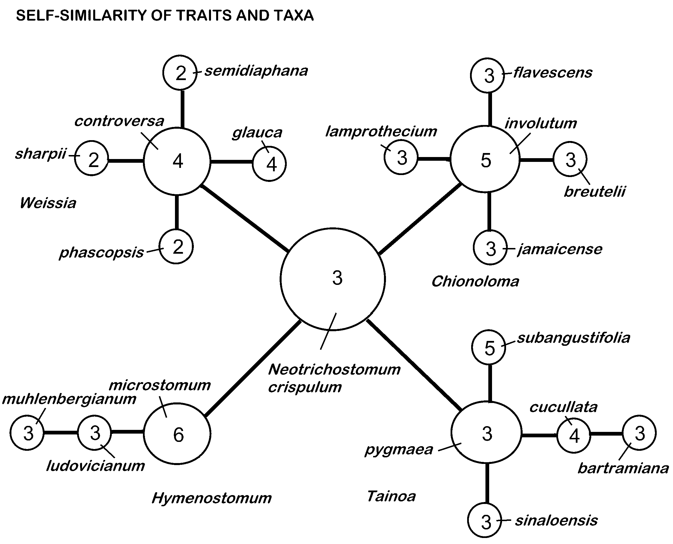
Figure 3.
Generalized fate of microgenera. A. A descendant of Genus 1 (red) generates about four descendants (green). B. Because all descendants have the novel traits of their ancestor, they are recognized as Genus 2 (green). C. Genus 2 may generate additional species from the immediate descendants (blue). D–G. Genus 2 gradually goes extinct.
Figure 3.
Generalized fate of microgenera. A. A descendant of Genus 1 (red) generates about four descendants (green). B. Because all descendants have the novel traits of their ancestor, they are recognized as Genus 2 (green). C. Genus 2 may generate additional species from the immediate descendants (blue). D–G. Genus 2 gradually goes extinct.
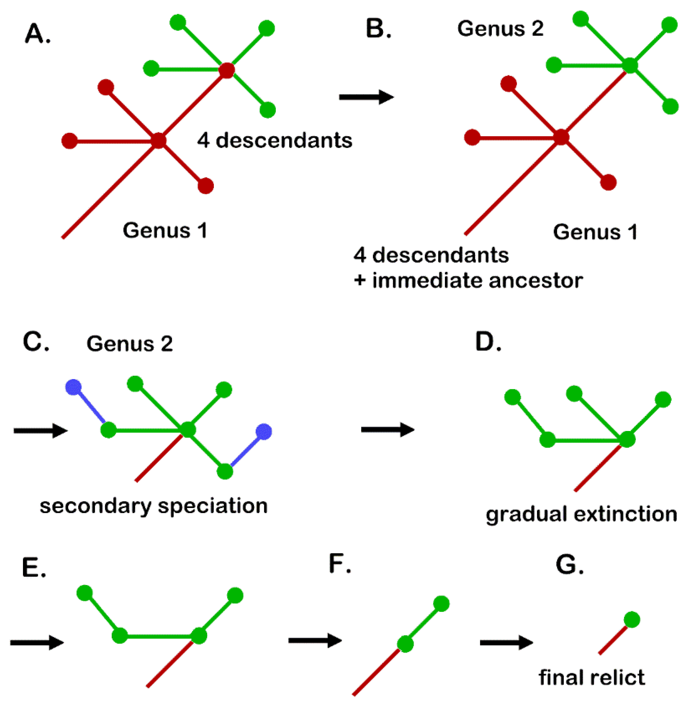
Figure 5.
Available evolutionary Force for initial impulse of selective force 4 for four descendant species, reflected in power-law numerator of 4. Red dashed line at x = 7 is the stalling point where available initial energy is used up as x increases energy drops by a factor of 1.14.
Figure 5.
Available evolutionary Force for initial impulse of selective force 4 for four descendant species, reflected in power-law numerator of 4. Red dashed line at x = 7 is the stalling point where available initial energy is used up as x increases energy drops by a factor of 1.14.
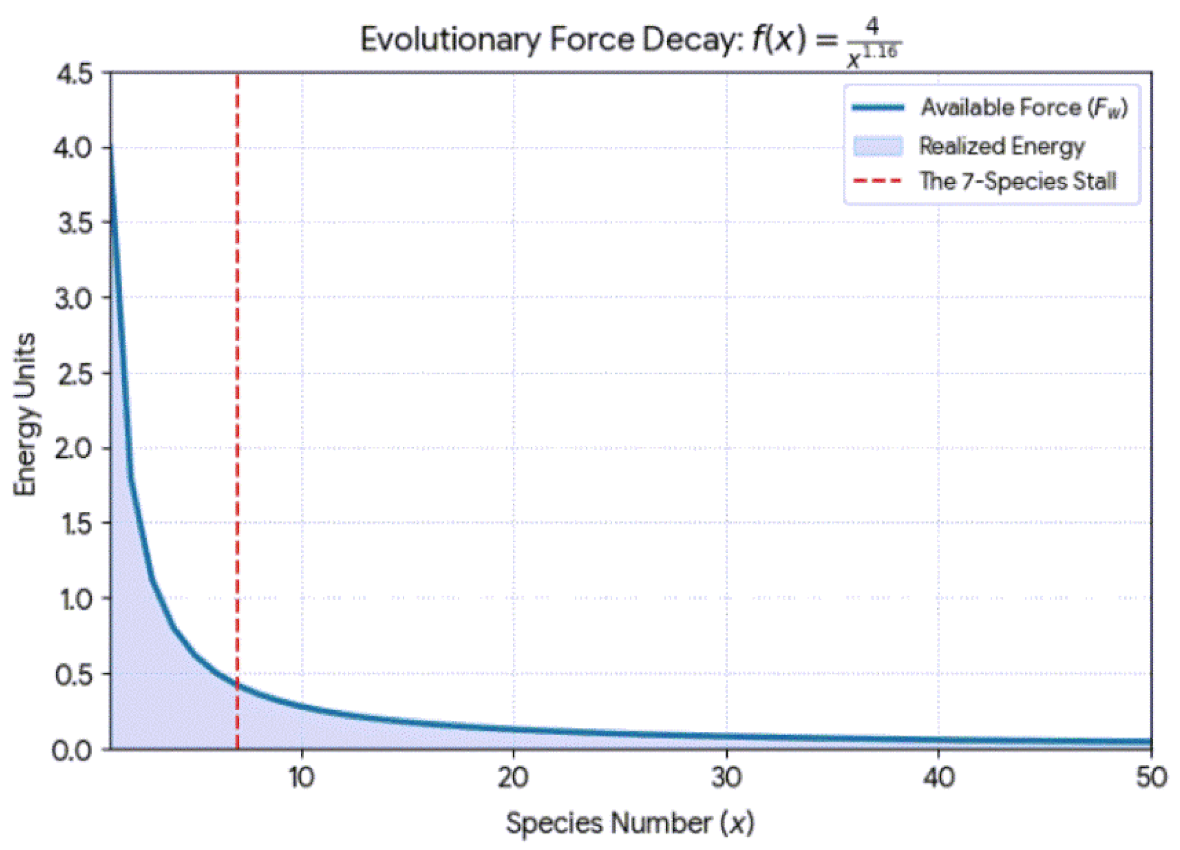
Figure 6.
Decay to stalling of evolutionary velocity showing solution to Equation 13. Numbers of species are per genus, with six descendants supported by available kinetic energy.
Figure 6.
Decay to stalling of evolutionary velocity showing solution to Equation 13. Numbers of species are per genus, with six descendants supported by available kinetic energy.
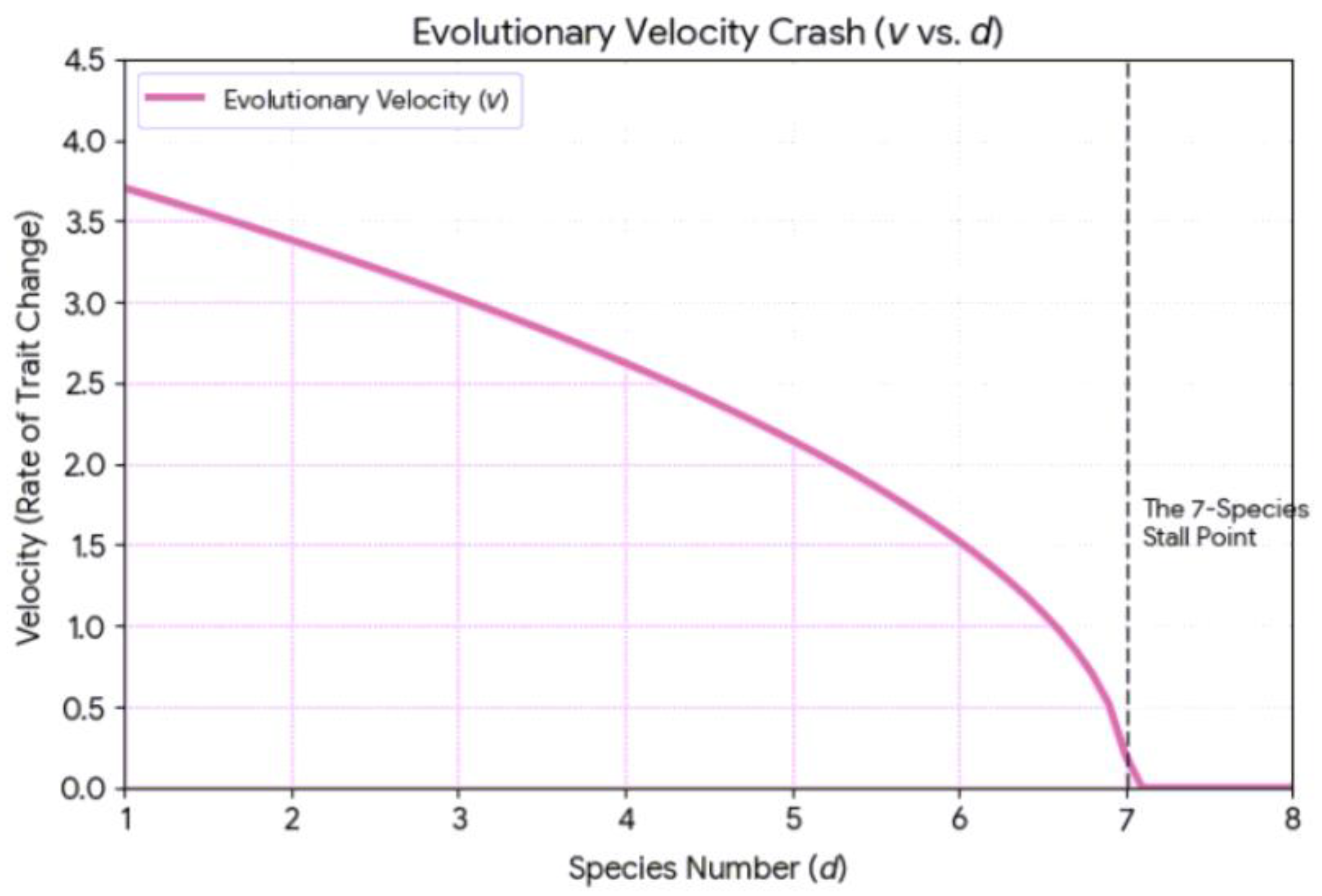

Table 1.
Spreadsheet caulogram of the bryophyte family Streptotrichaeceae. Numbers in header show sequential species events. Color coding distinguishes genera. Each column represents a speciation event. IEG is inferred extinct genus. Numbers in squares are morphological trait (character-state) changes for one speciation event.
Table 1.
Spreadsheet caulogram of the bryophyte family Streptotrichaeceae. Numbers in header show sequential species events. Color coding distinguishes genera. Each column represents a speciation event. IEG is inferred extinct genus. Numbers in squares are morphological trait (character-state) changes for one speciation event.
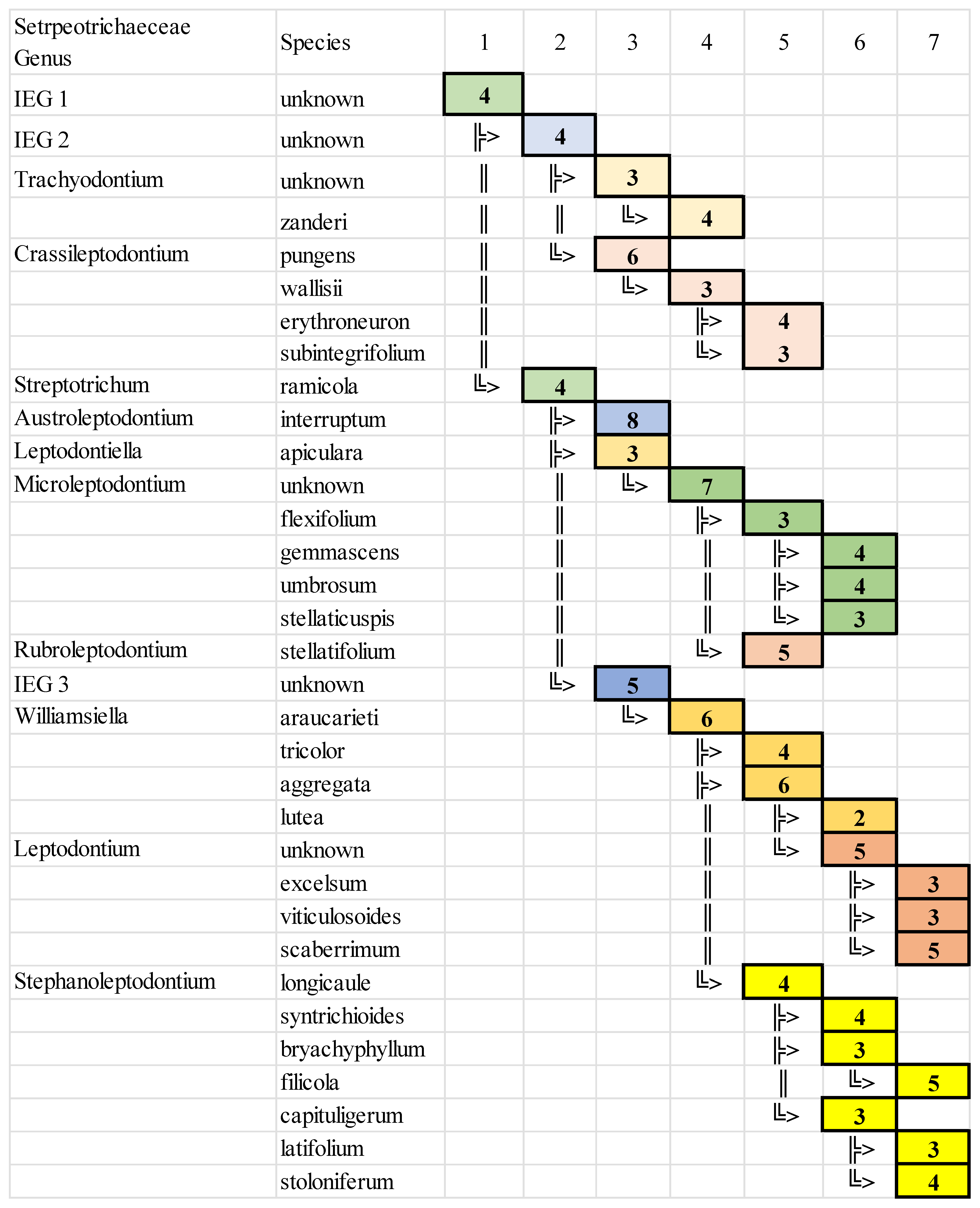 |
Table 2.
Spreadsheet caulogram of the rated moss Pottiaceae tribe Pleuroweisieae. Caption is the same as that for Table 1.
Table 2.
Spreadsheet caulogram of the rated moss Pottiaceae tribe Pleuroweisieae. Caption is the same as that for Table 1.
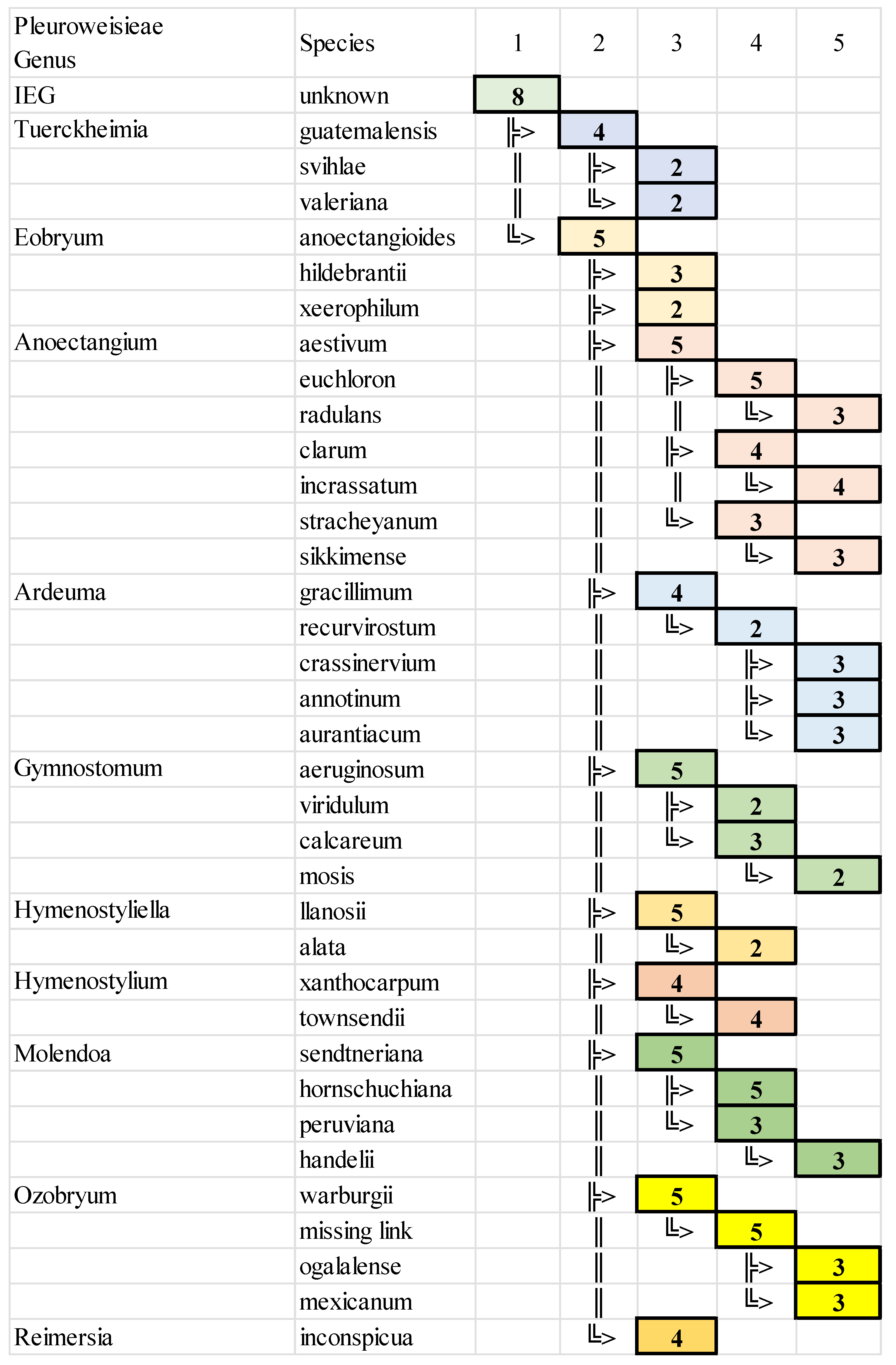 |
Table 3.
Physics analogues for evolutionary mechanics.
| Term and abbreviation | Physics analogue | Evolutionary Definition |
| Evolutionary mass (m) | Inertia | 1 species, or resistance to change. |
| Evolutionary distance (d) | Displacement | Total evolutionary path since taxon origination; total sum of trait changes in a caulon. |
| Evolutionary time | Steps | Speciation events |
| Evolutionary velocity (v) | Rate of innovation | Number of traits changed per speciation event; current speed of adaptation. |
| Evolutionary force (F) | Net force (F = ma) | Magnitude of selective pressure accelerating the rate of change; a jump in rate of change. |
| Kinetic energy (KE) | Evolutionary momentum, high KE implies rapid change; a scalar; the state of the energy. | |
| Potential energy (PE) | F × Δd | Adaptive tension, pressure for future trait changes by an environmental shift; a vector. |
| Work (W) | F × d | Total environmental effort to reach that state; the transfer of energy. |
| Total energy (E) | KE + PE | Total evolutionary energy of the taxon. |
| Taxonomic Action Unit (TAU) | Selective force × d, which is same as traits2/event2 | Energy required for 1 species (m=1) to undergo 1 trait change (v = 1) in 1 speciation event; evolutionary equivalent to joule (newton × meter); a change in momentum. |
| Punctuational impulse (J) | F × t, or Δmv | A strong single selective force originating a burst of species. |
| Constant of resistance or friction (k) | Dissipative force, selective pressure | Coefficient giving loss of energy due to niche-filling, competition and extinction; traits/event2. |
| Efficiency ratio (η) | Useful energy | Percent of Work output as kinetic energy. |
Table 4.
Spreadsheet data on Streptotrichaceae caulogram. TotrCa is summed new traits or evolutionary distance in the caulon. ToEvSp is total number of speciation events leading to that species. InVel is instantaneous velocity (changed traits) of species at last species event. CuVel is cumulative velocity or total velocity divided by number of species events. AccIns is instantaneous acceleration (plus or minus change in distance (changed traits) of last species at that speciation event. ToAcGe is total acceleration of all species in the genus. Work is Force times distance or total acceleration times total distance. KE is kinetic energy or 0.5 times one species times velocity squared.
Table 4.
Spreadsheet data on Streptotrichaceae caulogram. TotrCa is summed new traits or evolutionary distance in the caulon. ToEvSp is total number of speciation events leading to that species. InVel is instantaneous velocity (changed traits) of species at last species event. CuVel is cumulative velocity or total velocity divided by number of species events. AccIns is instantaneous acceleration (plus or minus change in distance (changed traits) of last species at that speciation event. ToAcGe is total acceleration of all species in the genus. Work is Force times distance or total acceleration times total distance. KE is kinetic energy or 0.5 times one species times velocity squared.
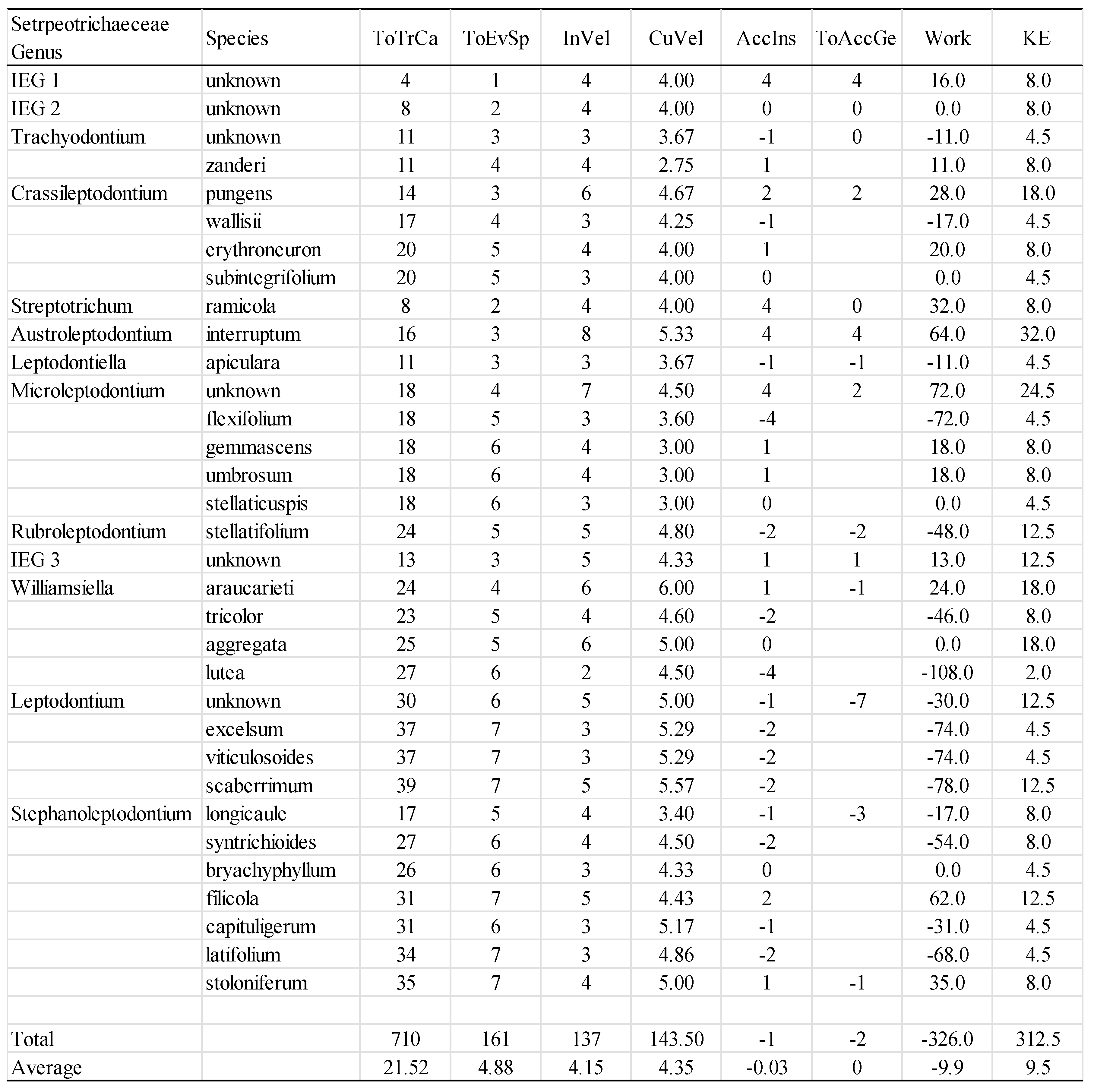 |
Table 5.
Spreadsheet data on Plueroweisieae caulogram. Table headings are the same as for Table 4.
Table 5.
Spreadsheet data on Plueroweisieae caulogram. Table headings are the same as for Table 4.
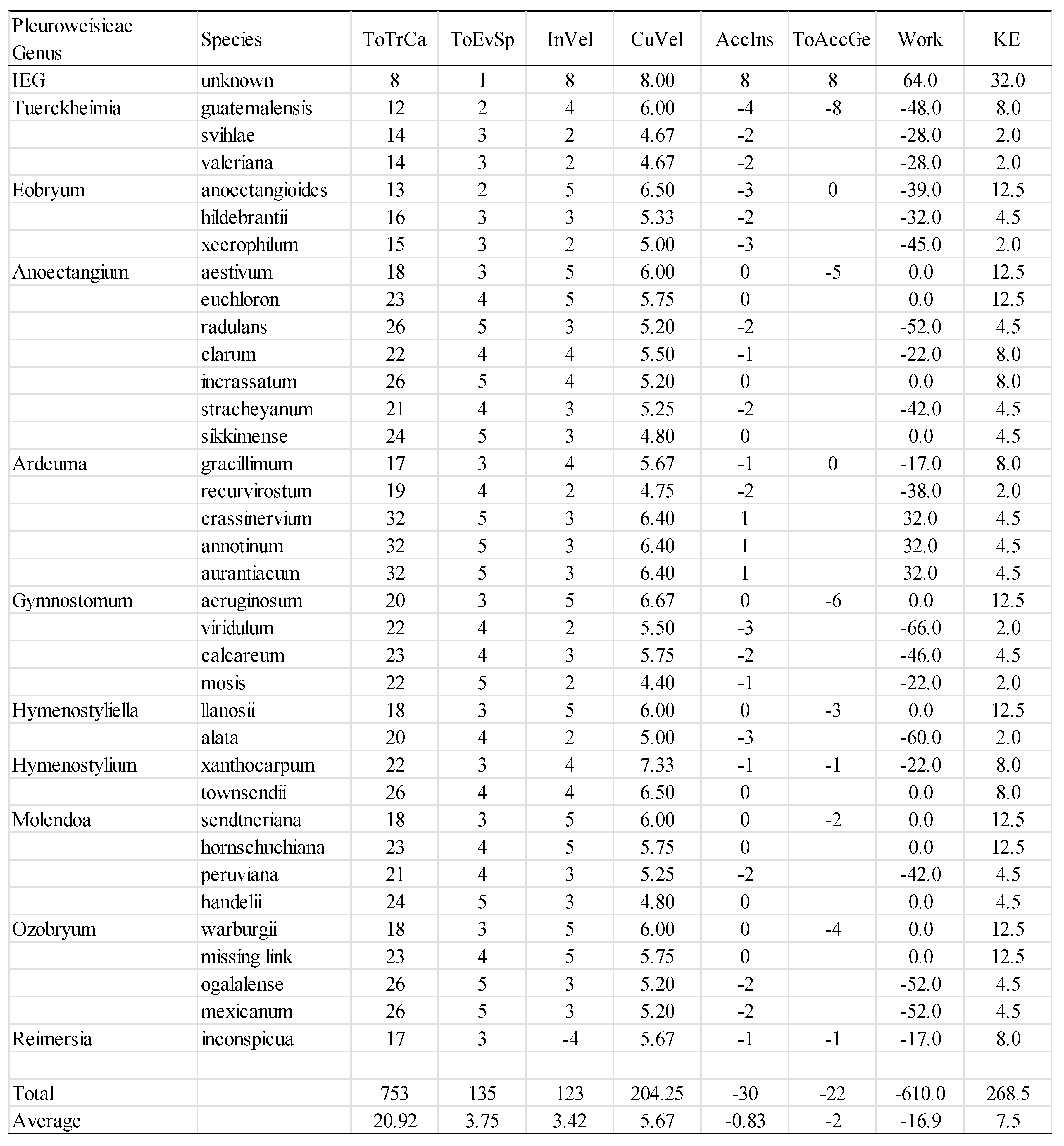 |
Disclaimer/Publisher’s Note: The statements, opinions and data contained in all publications are solely those of the individual author(s) and contributor(s) and not of MDPI and/or the editor(s). MDPI and/or the editor(s) disclaim responsibility for any injury to people or property resulting from any ideas, methods, instructions or products referred to in the content. |
© 2026 by the authors. Licensee MDPI, Basel, Switzerland. This article is an open access article distributed under the terms and conditions of the Creative Commons Attribution (CC BY) license (http://creativecommons.org/licenses/by/4.0/).
Copyright: This open access article is published under a Creative Commons CC BY 4.0 license, which permit the free download, distribution, and reuse, provided that the author and preprint are cited in any reuse.