
Submitted:
24 March 2026
Posted:
25 March 2026
You are already at the latest version
Abstract
Small streams exhibit rapid and nonlinear flood responses due to steep slopes, short flow paths, and limited storage capacity, making real-time flood prediction challenging under both computational and data constraints. This study proposes an integrated, measurement-based flood prediction framework that enables real-time estimation of flood dis-charge and flood depth in small-stream basins. Unlike conventional approaches that rely on either computationally intensive hydrodynamic models or standalone data-driven methods, the proposed framework combines high-frequency monitoring data, rainfall nowcasting, and nonlinear regression-based hydraulic relationships into a unified system. Rainfall–discharge nomographs and depth–discharge rating curves were developed using a nonlinear four-parameter logistic (4PL) regression model based on long-term observations from twelve representative basins in Korea. Forecast rainfall from the Korea Meteorological Administration MAPLE nowcasting system was used to estimate discharge, which was subsequently transformed into flood depth through calibrated rating curves. To extend prediction capability beyond monitoring locations, additional depth–discharge relationships were derived for ungauged reaches using hybrid approaches based on HEC-RAS scenario simulations and the Manning equation. Validation against major flood events showed strong agreement between observed and predicted values, with mean prediction accuracies of approximately 89% for discharge and 90% for flood depth. The proposed framework effectively captures nonlinear rainfall–runoff behavior while significantly reducing computational complexity compared with conventional hydrodynamic models. These results demonstrate that the framework provides a practical and scalable solution for real-time flood prediction and early warning in small-stream environments, particularly by enabling spatially continuous flood-depth estimation across both gauged and ungauged reaches.
Keywords:
real-time flood prediction
; small streams
; rainfall–discharge nomograph
; depth–discharge rating curve
; flood early warning
1. Introduction
Localized extreme rainfall has intensified in both magnitude and occurrence in recent years, increasing flood damage in small-stream basins. Because these streams are generally located in upstream areas, they commonly have steep bed slopes, short flow paths, narrow channel sections, and rapidly varying hydraulic conditions. Such characteristics accelerate flood-wave propagation and increase exposure to sweep-out accidents, thereby contributing to a high proportion of flood-related casualties. Recent studies have highlighted the seriousness of flood hazards in small streams. Cheong, et al. [1] reported that approximately 42.3% of flood-related fatalities within river basins in Korea occurred in small streams. In addition, economic losses of about USD 193 million were recorded in 5013 small streams between 2020 and 2024, accounting for 22.7% of the national total. Despite these growing risks, operational flood forecasting and warning systems have historically focused on larger downstream rivers, leaving small-stream basins relatively underrepresented.
Flood forecasting has traditionally relied on numerical hydraulic models; however, their direct application to small streams remains challenging. Irregular channel geometry and steep longitudinal slopes increase sensitivity to model parameters and boundary conditions during flood events, which can reduce numerical stability and simulation reliability [2,3,4,5]. In addition, discharge and flow velocity in these basins can change abruptly over short time scales. Accurate simulation of such behavior requires fine spatial discretization and short computational time steps [6], which limits the practicality of real-time forecasting and rapid emergency response under fast-changing hydrological conditions [7,8,9]. These limitations highlight the need for alternative flood prediction approaches that can simultaneously achieve computational efficiency, predictive accuracy, and real-time applicability in small-stream environments. In this context, measurement-based flood forecasting methods have emerged as promising alternatives or complements to conventional numerical modeling by directly utilizing real-time observational data.
These constraints indicate the need for alternative forecasting methods that can provide both computational efficiency and acceptable predictive accuracy in small-stream environments. In this regard, measurement-based and data-driven approaches have emerged as promising complements to conventional hydrodynamic modeling because they directly utilize real-time observations. A practical measurement-based forecasting system requires three key elements: (i) prediction models that are sufficiently accurate while remaining computationally efficient for operational use; (ii) seamless linkage between these models and real-time monitoring systems for rapid data assimilation; and (iii) a stable platform for data collection, storage, and management. Long-term monitoring data are particularly important in small-stream basins, where rainfall–runoff behavior often exhibits pronounced temporal and spatial variability. Continuous observations covering seasonal conditions, and a wide range of rainfall intensities can improve model robustness and predictive reliability [10,11]. On this basis, to address these limitations, this study proposes an integrated, measurement-based flood prediction framework that links real-time observations, rainfall nowcasting, and nonlinear hydraulic relationships to enable rapid and spatially continuous flood prediction in small-stream basins.
2. Materials and Methods
2.1. Selection of Test-Bed Small-Streams
To support the development and validation of the flood prediction model, the research used real-time observational data collected from the Small-stream Smart Monitoring and Management System (SMMS). Unlike conventional in situ measurement methods, the SMMS uses image- and radar-based non-contact techniques to continuously monitor surface velocity distributions and to automatically estimate discharge in real time [7,12,13,14]. The measured flood depth and discharge data were incorporated directly into the prediction framework for calibration and validation, thereby improving forecasting reliability [1,15,16,17]. Previous studies have shown that observation-based flood forecasting can provide rapid and accurate estimates of flood-wave propagation and inundation potential in river systems [10,18,19].
At the time of this study, the Ministry of the Interior and Safety and local governments in Korea had deployed the SMMS at approximately 880 locations, with a long-term plan to install the system in about 2,200 small streams, corresponding to roughly 10% of the 22,300 small streams nationwide. For model development and evaluation, twelve test-bed small streams with observational records longer than three years were selected. Flood depth and discharge were available at 2 min intervals for all selected sites. The test-bed streams were Insu, Neungmac, Bekam, Songnam, Balmak, Jungdong, Jumsil, Gumanri, Daemi, Gwangdong, Jungsunpil, and Sunjang. The average longitudinal slope of the twelve streams was 0.029, indicating relatively steep hydraulic conditions. Their mean channel length was 2.34 km, which reflects the short spatial scale typical of small streams. Channel width ranged from 6.80 to 24.0 m, with an average of 15.62 m, confirming the narrow-channel characteristics of the study sites.
Rainfall input data were obtained from the Automated Weather Station (AWS) network operated by the Korea Meteorological Administration (KMA). More than 510 AWS stations are operated nationwide to provide continuous meteorological observations for disaster prevention and early warning. These stations offer detailed temporal and spatial information on rainfall distribution, thereby supporting rainfall-based forecasting systems [20]. In this study, minute-scale rainfall data from the AWS station nearest to each SMMS-equipped stream were selected and incorporated into the modeling framework. The monitoring locations, SMMS installation information, basin area (), channel length (), channel width (), channel slope (), roughness coefficient (), designed discharge (), designed depth (), and the distance between each stream and the nearest AWS station () are summarized in Table 1.
As shown in Figure 1, watershed areas and channel lengths were delineated from satellite imagery by defining the upstream and downstream boundaries of each stream. GIS tools were then used to derive watershed slope and topographic characteristics to ensure that basin geometry was represented consistently.
In addition to observation quality, the reliability of forecast rainfall was also critical for accurate flood prediction in small streams, as emphasized in recent studies on short-term rainfall forecasting for flood modeling and early warning [1,21,22]. The KMA estimates short-term rainfall movement and variability using AWS observations and weather radar data, which have been shown to improve nowcasting performance in hydrological applications [23]. Based on this system, the KMA provides gridded rainfall forecasts nationwide at 10 min intervals with lead times of up to 6 h. In this study, these forecast rainfall data were used to support proactive flood response in small-stream watersheds [24,25].
For model development and validation, flood depth, discharge, and rainfall data were collected from the SMMS and AWS networks from 2016, when the first monitoring system was installed, through 2025. Summary statistics of the collected data are presented in Table 2. Because the selected streams are largely ephemeral during dry periods, minimum values were excluded to focus on hydrologically meaningful conditions relevant to flood analysis and model evaluation [1,26]. Across the test-bed watersheds, mean annual rainfall ranged from 1180.1 to 1588.2 mm. Rainfall was concentrated mainly during the summer season from June to September, consistent with recent analyses of sub-daily heavy rainfall characteristics in Korea based on dense surface observations [27].
As shown in Table 2, the maximum 1-h rainfall intensity varied substantially among the study streams, ranging from 33.5 at Jumsil stream to 95.8 at Sunjang stream. This pattern is consistent with previous findings that short-duration extreme rainfall in Korea exhibits marked regional and seasonal heterogeneity [28]. Peak discharge, which is commonly used to characterize rainfall–runoff behavior in small basins, ranged from 4.98 at Jungdong stream to 210.3 at Sunjang stream. This wide range reflects the rapid and highly nonlinear hydrologic and hydraulic responses typical of small streams and further supports the need for data-driven, real-time forecasting frameworks based on high-frequency monitoring data [10].
A similarly wide range was observed for peak flow depth, from 0.46 m at Balmak stream to 2.45 m at Sunjang stream. These results underscore the importance of site-specific early warning strategies supported by observed hydraulic data. Overall, the mean and maximum values summarized in Table 2 provide useful baseline information for interpreting flood magnitude and flow regime characteristics in the test-bed streams and for supporting event-scale model calibration and validation [1].
2.2. Data Collection and Analysis
To make effective use of high-frequency monitoring data, this study developed a Flood Early Warning Platform (FEWP) that automatically collected rainfall, water level, and discharge data from the SMMS and AWS networks and stored them in a structured database for integrated analysis and operational flood forecasting [29,30]. Previous studies have shown that real-time integration of sensor networks with hydrometeorological monitoring systems is essential for operational early warning because it reduces data latency and improves forecast performance [31,32].
An AI-assisted flood prediction module was developed and integrated into the FEWP to establish a unified operational workflow linking real-time observational data streams with predictive analytics. This integration enabled faster dissemination of forecast information on flood occurrence and potential impacts to decision-makers and stakeholders [29,33]. AI-based prediction frameworks have been reported to improve early warning capability by assimilating heterogeneous real-time datasets and by capturing nonlinear hydrological responses through machine-learning algorithms [33]. Accordingly, the FEWP was designed to support rapid flood detection, forecasting, and information delivery under increasingly severe hydrological and climatic conditions. Real-time data assimilation combined with predictive analytics has become a key component of next-generation flood early warning systems, particularly in monitoring environments characterized by dense, high-frequency observations [29,32].
3. Flood Prediction Methods and Procedure
Flood forecasting in small streams requires rapid model execution to provide actionable lead time despite short watershed response times and high flow velocities [10,34]. To estimate both discharge and flood depth, this study developed separate but linked procedures for gauged and ungauged reaches, as illustrated in Figure 2.
For gauged reaches, the relationship between peak rainfall intensity observed at nearby AWS stations and peak discharge measured by the SMMS was analyzed. Based on this relationship, a four-parameter rainfall–discharge nomograph was established as expressed in Equation (1).
in which denotes observed flood discharge, denotes observed rainfall intensity, and , , , and are parameters estimated using a nonlinear optimization technique. A 60 min rainfall intensity was adopted because the time of concentration for many small streams is approximately one-hour [7].
The observed rainfall and discharge records were separated into individual flood events, and the temporal distribution of each event was examined. For each event, the peak rainfall intensity and corresponding peak discharge were extracted and treated as one rainfall–discharge pair. Repeating this procedure for all identified events produced the dataset required to calibrate the rainfall–discharge nomograph through nonlinear optimization. Similar relationships have long been used as practical tools for converting hydrological input into discharge estimates [2,7,35,36,37].
3.1. Method for Gauged Reaches
Flood depth at gauged reaches was estimated using a four-parameter depth–discharge rating curve, as expressed in Equation (2), developed from the relationship between observed peak discharge and peak flood depth.
in which is the observed flood depth, and , , , and are parameters estimated using a nonlinear optimization technique. To construct this relationship, the observed discharge and water-depth records were also separated into individual flood events, and the peak discharge and corresponding peak depth were extracted for each event. These peak pairs were then used in nonlinear regression to derive the depth–discharge rating curve. Such rating curves provide a concise representation of hydraulic response and are widely used to estimate flood depth from discharge [1,2,38,39].
To estimate discharge and depth using the nomograph and rating curve, an objective function was defined to minimize the difference between observed and predicted values, as expressed in Equation (3).
in which F(x) denotes the optimal predicted value, represents the observed value at time , and indicates the predicted value at time . Real-time forecast rainfall from the KMA MAPLE nowcasting system was used as the input for the rainfall–discharge nomograph. Forecast rainfall intensities were extracted from the same grid cells corresponding to the AWS locations used during model calibration. The resulting predicted discharge was then converted into flood depth through the depth–discharge rating curve.
During prediction, simulated values were iteratively compared with observations until the prediction error reached a minimum. In each iteration, the predicted discharge and depth were used to update the rainfall–discharge nomograph and the depth–discharge rating curve, as shown in Figure 3. These updated relationships were then carried forward to the next iteration. This sequential updating process improved the final estimates of flood discharge and flood depth.
The nonlinear least-squares problem was solved using the Levenberg–Marquardt (LM) method, which is widely known for numerical stability and rapid convergence [40,41,42,43]. The LM method is commonly used for nonlinear optimization problems such as Equation (3) and can be interpreted as a damped variant of the Newton–Raphson method, as expressed in Equation (4).
in which denotes the parameter vector at the k-th iteration, and is the Hessian matrix, representing the second-order partial derivatives of the objective function. Optimization methods that directly compute the Hessian may suffer from divergence and can be computationally expensive. The LM method avoids this difficulty by locally approximating the objective function with a linear form. Under this assumption, the parameter update is obtained from Equation (5).
in which J denotes the Jacobian matrix of the residual vector with respect to the parameter vector . The term serves as an approximation of the Hessian matrix . Thus, the LM method estimates values close to the optimum by repeatedly computing the update vector at each iteration. In the present framework, the update vector for discharge and depth estimation is expressed by Equation (6).
in which is the diagonal matrix of , and is the damping parameter at the k-th iteration, which is determined by the gain ratio as defined below.
in which is the objective function locally approximated around . The initial damping parameter was initially set to , and the damping value was updated at each iteration following the adaptive strategy proposed by Marquardt [41].
The flood depth predicted through this process was limited to the gauged reaches within the entire river network; therefore, additional methods were required to estimate flood depth in ungauged reaches.
3.2. Method for Ungauged Reaches
To estimate flood depth in ungauged reaches, this study used depth–discharge relationships derived from both the Manning equation and HEC-RAS simulations, as illustrated in Figure 4. Flood depth predicted at gauged locations reflects hydraulic conditions only at monitoring points and therefore does not fully represent flood risk along the entire stream reach. In reaches with low levee elevations or structural vulnerability, depth predictions at a single gauged location may be insufficient to assess overflow and inundation risk. Consequently, reliable depth estimation across the full stream length is needed for practical flood-risk identification, as frequently requested by local practitioners responsible for small-stream management.
The applicability of HEC-RAS for ungauged small-stream reaches was first examined. The analysis indicated that steep slopes and short flow lengths can limit the ability of HEC-RAS to reproduce hydraulic variability adequately under real-time conditions [1,44,45,46]. Direct real-time application was therefore considered susceptible to numerical instability. To address this limitation, scenario-based simulations were conducted in advance, and peak discharge–depth pairs were generated under different upstream discharge and downstream water-level boundary conditions. According to HEC-RAS guidance from the U.S. Army Corps of Engineers, shallow-water simulations can become unstable in reaches with slopes greater than 1%. Recommended measures include reducing the computational time step or increasing Manning’s roughness coefficient . These measures were considered in the scenario design used in this study.
For this purpose, detailed cross-sectional survey data were collected for each pilot stream reach. These data were used to represent channel geometry, levee configuration, bed slope, hydraulic radius, and variations in flow depth. Fine-resolution measurements of horizontal spacing and elevation across each section enabled accurate representation of cross-sectional area and effective flow width. Based on the simulated peak discharge and depth values, depth–discharge relationships were developed for each reach using the same procedure adopted for gauged reaches. Predicted discharge was then used as input to estimate flood depth along ungauged reaches. In doing so, discharge was assumed to remain constant along the stream due to the absence of tributary inflow. This assumption is considered reasonable because most of the selected small streams in Korea do not receive substantial tributary inflow.
A second ungauged-reach approach was based on the Manning equation. The Manning equation estimates flow depth and velocity from discharge, channel slope, roughness coefficient, and hydraulic geometry, allowing continuous reach-wise prediction of flood depth [47,48]. However, because this method treats each reach independently, it may underestimate depth in steep channels [33,49,50]. Previous studies have reported that direct estimation of Manning’s roughness coefficient using deep-learning models trained on flume data can reduce errors in simulated flood depth and inundation extent in one-dimensional flood models [49]. It has also been shown that combining remote sensing information, such as synthetic aperture radar data, with terrain information and machine learning can further improve depth estimation by refining the estimation of Manning’s [51,52].
In this study, optimal roughness coefficients for the Manning-based calculations were determined through field surveys, and the resulting values are listed in Table 1. Cross-sectional survey data were also collected for each test-bed stream reach, and the corresponding cross-sectional area and hydraulic radius were calculated. Reach-scale geometric characteristics are presented in Figure 4.
4. Development of Flood Prediction Methods
4.1. Prediction Method for Gauged Reaches
Rainfall–discharge nomographs and depth–discharge rating curves are practical statistical and hydraulic relationships used to estimate discharge and flow depth from rainfall intensity and discharge, respectively [10,53,54]. In this study, both relationships were represented using a nonlinear four-parameter logistic (4PL) regression model, as defined by Equations (1) and (2). The 4PL model is well suited to nonlinear phenomena and is particularly effective for representing curved relationships commonly observed in hydraulic and hydrological datasets [55,56]. The 4PL model was selected due to its ability to represent nonlinear asymptotic behavior.
To construct the rainfall–discharge nomographs, 1-min rainfall records measured from 2022 to 2025 at the AWS stations nearest to the twelve study streams were converted into 60 min accumulated rainfall intensity series. These rainfall series were analyzed together with the 2-min discharge data measured by the SMMS. For each flood event, the peak rainfall intensity and corresponding peak discharge were extracted. To derive the depth–discharge rating curves, peak flood depth and the corresponding peak discharge were similarly extracted from the observed depth and discharge records. Repeating this procedure for each event in each of the twelve streams produced datasets of rainfall intensity–discharge pairs and discharge–depth pairs. These datasets were then used in nonlinear 4PL regression to derive the rainfall–discharge nomographs and depth–discharge rating curves. The resulting parameter estimates and coefficients of determination are summarized in Table 3. In all cases, the fitted relationships showed high coefficients of determination, approaching 0.99.
To evaluate the goodness of fit, scatter plots of peak rainfall intensity versus peak discharge and peak depth versus peak discharge were compared with the fitted 4PL curves, as illustrated in Figure 5. Although watershed characteristics such as drainage area, land use, and surface cover varied among the twelve streams, the fitted relationships showed consistent patterns across the monitored basins. This suggests that the developed relationships are not restricted to only one specific site but may be applicable to small streams that fall within a similar range of watershed characteristics.
McCuen [54] noted that a single empirical equation may be insufficient to represent the combined effects of rainfall–runoff response, infiltration, and topographic controls. To reduce the uncertainty associated with simple empirical formulas, this study used multivariate calibration based on more than four years of observed rainfall, discharge, and depth data. This framework was designed to account simultaneously for spatiotemporal rainfall–runoff variability and watershed properties such as slope, land cover, and channel alignment. As a result, the calibrated relationships showed very strong agreement with measured discharge and depth and reduced statistical error relative to simpler regression-based estimation methods.
4.2. Prediction Method for Ungauged Reaches
For ungauged reaches, peak discharge–depth pairs were generated using HEC-RAS steady-flow scenario simulations, and depth–discharge rating curves were subsequently fitted using the same 4PL regression approach applied to gauged reaches. These relationships provide a practical basis for estimating flood depth in ungauged reaches from discharge predicted at gauged locations. Depth–discharge rating curves derived from the HEC-RAS scenarios were developed for all ungauged reaches in the twelve test-bed streams. However, because of space limitations, only the fitted parameters and coefficients of determination for Jungdong stream, which has the shortest channel length among the study streams, are presented in Table 4.
Application of the nonlinear 4PL regression model to the simulated data produced very high coefficients of determination for the ungauged reach rating curves, ranging from 0.987 to 0.999, as shown in Table 4. To illustrate the fit, the scatter plot of simulated peak depth versus peak discharge for Jungdong stream was compared with the corresponding fitted curve in Figure 6.
As shown in Figure 6, the ungauged-reach depth–discharge relationships reproduced the simulated depth–discharge patterns with very strong agreement. This result indicates that regression-based calibration of scenario outputs can provide an efficient approximation of hydraulic behavior while reducing statistical error relative to simpler predictive approaches.
4.3. Application of Forecast Rainfall
Forecast rainfall used for small-stream prediction was obtained from the KMA MAPLE nowcasting system. MAPLE provides gridded rainfall forecasts at a spatial resolution of 1 km and generates 36 forecast fields at 10-min intervals, allowing lead times of up to 6- h. In this study, rainfall values were extracted from the grid cells containing the AWS locations for each of the twelve streams and used as forecast rainfall input.
To examine the influence of lead time on forecast performance, the largest flood event for each of the twelve streams was selected. The maximum events occurred on 9 August 2022 for Insu stream; 5 September 2023 for Neungmac, Jungsunpil, and Sunjang streams; 13 July 2023 for Daemi and Jumsil streams; 20 September 2023 for Bekam stream; 26 June 2023 for Gwangdong stream; 17 July 2023 for Balmak stream; 14 July 2023 for Songnam stream; 23 July 2023 for Jungdong stream; and 21 June 2023 for Gumanri stream. To evaluate forecast applicability, differences between observed and forecast peak rainfall intensity were analyzed for lead times from 10 min to 6 h. The results are presented in Figure 7.
In general, forecast accuracy tends to decrease, or at best remain similar, as lead time increases [57,58]. However, the present results indicate that forecast rainfall could be either underestimated or overestimated relative to observations, and the magnitude of the error did not increase monotonically with lead time. Instead, the error fluctuated as lead time increased. Based on these results, the 1-h ahead forecast was selected for discharge prediction because it showed relatively high accuracy and was consistent with the short response time of small streams. Therefore, a 1-h forecast horizon was considered appropriate for real-time flood prediction in the study basins [59].
5. Application of Flood Prediction Methods
5.1. Application of Prediction Method for Gauged Reaches
To validate the developed framework, predicted discharge and flood depth were compared with the corresponding observations measured by the SMMS at the twelve test-bed streams. Major flood events occurring in 2022 and 2023 were selected for evaluation. As shown in Figure 8, the model reproduced the temporal variation of both discharge and depth with good agreement.
The validation results indicate that the calibrated rainfall–discharge nomographs and depth–discharge rating curves can represent the hydrological and hydraulic response characteristics of the study streams effectively, thereby improving prediction performance [60,61]. In the present study, 60 min accumulated rainfall intensity was used to construct the rainfall–discharge nomograph because hourly rainfall best reproduced the observed discharge variation in the selected small streams and has also been recognized as a useful indicator of flood occurrence in both urban and rural watersheds [53,62].
The depth–discharge rating curve was calibrated using peak discharge and peak depth data, enabling the model to reproduce observed peak water levels with relatively small error. These results suggest that the proposed approach can be used not only to estimate discharge but also to track flood-stage variation during event periods. To quantify the difference between observed and predicted values, a discrepancy ratio was defined as follows:
in which is discrepancy ratio, is predicted values and is measured values. To compare the distribution of discrepancy ratios for predicted discharge and flood depth at each stream, the values were grouped into intervals of 0.01 within the range of −0.05 to 0.05, intervals of 0.05 up to 0.1, and intervals of 0.1 up to 0.2. The frequencies in each interval were then converted to percentages and presented as histograms in Figure 9 and Figure 10.
The validation results show that discrepancy ratios for both discharge and depth generally followed a near-normal distribution. For all twelve streams, the ratios ranged from −0.2 to 0.2, with the highest frequency occurring within −0.01 to 0.01. To compare performance among sites, prediction accuracy was defined as the proportion of discrepancy ratios falling within −0.01 to 0.01. The resulting accuracy values for discharge and depth are summarized in Table 5.
For discharge prediction, the highest accuracy, 100%, was obtained for Insu, Bekam, and Jungsunpil streams, whereas the lowest value, 73.92%, was found for Gumanri stream. For water-depth prediction, the highest accuracy, 100%, was achieved for Insu, Gwangdong, Jungsunpil, and Sunjang streams, whereas the lowest value, 74.86%, again occurred at Gumanri stream. Overall, the mean accuracy of water-depth prediction was slightly higher than that of discharge prediction, indicating that the proposed framework estimated flood depth somewhat more reliably than discharge. Streams with discharge prediction accuracy below the overall mean included Songnam, Jungdong, Gumanri, Gwangdong, and Sunjang, whereas Neungmac, Songnam, Jungdong, Gumanri, and Daemi showed below-average performance in water-depth prediction.
To further quantify prediction performance, RMSE was also calculated and is summarized in Table 5. For discharge prediction, the smallest RMSE values were observed at Insu and Neungmac streams (0.0003 ), whereas the largest was found at Daemi stream (1.1534 ). For water-depth prediction, the smallest RMSE was recorded at Jungsunpil stream (0.0003 ), while the largest occurred again at Daemi stream (0.0518 ). On average, RMSE was lower for flood depth than for discharge, further supporting the conclusion that the present framework reproduces flood depth more accurately than discharge in the selected basins.
5.2. Application to Ungauged Reaches
The observation-based prediction framework was successfully applied at gauged reaches equipped with the SMMS, allowing proactive response based on predicted flood conditions. However, monitoring devices are not available along all stream segments, and inundation can occur in ungauged reaches. The twelve streams considered in this study range in length from 0.5 to 13.63 km, which means that substantial portions of the channels remain ungauged. For this reason, an additional flood-depth estimation procedure was developed for ungauged reaches. This need has also been consistently emphasized by local government officials responsible for small-stream disaster management.
To support practical emergency response, the ungauged-reach model was designed to identify hazardous reaches in advance and to assist evacuation and warning decisions. Detailed cross-sectional geometry for major channel sections was obtained from Comprehensive Small Stream Maintenance Plan reports prepared by local governments at ten-year intervals. Using these data, flood depth along ungauged reaches was estimated through section-specific depth–discharge rating curves derived from HEC-RAS scenarios and from the Manning equation. The discharge used in these calculations was obtained from the gauged reaches through the rainfall–discharge nomograph, and tributary inflow was assumed to be negligible so that discharge remained constant along the stream. Figure 11 compares flood depths predicted using the Manning equation with those estimated using HEC-RAS-based rating curves.
The results for the twelve streams indicate that flood depths predicted by the Manning equation generally followed trends like those produced by the HEC-RAS scenario-based approach. However, in coastal streams such as Songnam and Jungdong, flood depths estimated from the HEC-RAS-based rating curves were slightly lower than those calculated using the Manning equation. Tidal river reaches are ideally analyzed using unsteady-flow models to estimate design flood depth [63]. In this study, however, steady gradually varied flow simulations were used because convergence problems occurred frequently in small streams, which may partly explain the observed differences.
To evaluate practical applicability, predicted flood depths based on the Manning equation were compared with levee-crest elevations to assess overtopping potential, as shown in Figure 12. No overtopping was predicted for any of the twelve streams, which is consistent with field observations indicating that no overtopping occurred during the study period. These findings support the applicability of the proposed model for real-time flood-depth estimation in ungauged reaches. Flood depths estimated from the HEC-RAS-based rating curves were also calculated, but these results were not plotted separately because they were nearly identical to those derived from the Manning equation and could not be easily distinguished graphically.
From an operational perspective, the Manning-based approach was advantageous for preliminary forecasting because of its simple structure and short computation time. However, its results were sensitive to uncertainties in bed slope and roughness estimation, which means that field survey and parameter calibration remain essential before practical application. Recent studies have also shown that spatiotemporal variability in Manning’s roughness coefficient is a major source of uncertainty in flood-level and inundation estimation [64,65].
As illustrated in Figure 11 and Figure 12, simplified Manning-based calculations can produce discontinuities in estimated flood depth between adjacent reaches or abrupt reductions in depth in steep channels because they do not fully account for hydraulic interactions such as upstream–downstream connectivity, backwater effects, hydraulic structures, and rapidly varied flow. Reach-by-reach computations may therefore underestimate flood levels when these controls are significant [66]. In steep small streams, the rapid propagation of flood waves and complex channel geometries required the application of hydrodynamic models based on the Saint-Venant equations rather than simplified empirical formulations [17,18]. However, although these models provide superior physical realism, they often require substantial computation time and operational complexity, which limits their usefulness in real-time forecasting [67,68,69,70].
By contrast, depth–discharge rating curves derived in advance from HEC-RAS scenarios require significant effort only during the initial setup stage. Once established, they allow rapid water-depth estimation during operational forecasting while preserving the dominant hydraulic characteristics of the flow system [71,72]. This approach reduces the unrealistic discontinuities that may arise in simplified methods and therefore offers a practical balance between hydraulic realism and computational efficiency. For this reason, the proposed framework is considered well suited to real-time flood-depth prediction in ungauged reaches of small streams and may serve as a useful basis for customized flood forecasting and warning systems [68,73].
6. Conclusions
This study proposed a measurement-based flood prediction framework for small streams by integrating real-time monitoring data with rainfall–discharge nomographs and depth–discharge rating curves. The framework was designed to address the limitations of conventional hydrodynamic models, which often require substantial computational effort and complex configuration and are therefore difficult to apply operationally in steep, short-response small-stream basins. By combining high-frequency monitoring data from the SMMS with rainfall observations and forecasts from the AWS network, the proposed framework provided a data-driven means of rapidly estimating both flood discharge and flood depth during event periods.
Using long-term observations from twelve test-bed small streams, rainfall–discharge nomographs and depth–discharge rating curves were developed through nonlinear four-parameter logistic regression. Because these relationships were derived directly from observed hydrological and hydraulic data, they were able to capture the nonlinear rainfall–runoff response characteristics of the monitored basins. The resulting framework enabled rapid transformation of forecast rainfall into flood discharge and subsequent conversion of discharge into flood depth while maintaining high computational efficiency.
Validation against major flood events showed that the proposed framework reproduced the temporal variation of both discharge and depth with good agreement. Mean prediction accuracy was approximately 89% for discharge and 90% for flood depth across the twelve streams. These results indicate that the calibrated relationships effectively represent the hydrological and hydraulic behavior of the monitored small streams and can reduce prediction error relative to simpler regression-based methods.
To extend the framework beyond gauged monitoring locations, additional flood-depth estimation procedures were developed for ungauged reaches using HEC-RAS-based scenario rating curves and the Manning equation. Both approaches produced broadly similar depth patterns, although the simplified Manning-based approach tended to underestimate depth in steep reaches because it does not fully account for hydraulic interactions such as backwater effects, rapidly varied flow, and channel-geometry changes. In contrast, the HEC-RAS-based scenario curves provided more consistent depth estimates by embedding reach-specific hydraulic characteristics into pre-established relationships. Comparison of predicted water levels with levee-crest elevations further showed that overtopping did not occur in any of the twelve streams during the analyzed events, consistent with field observations.
Overall, the proposed framework offers a practical and computationally efficient approach for real-time flood prediction in small streams. By linking real-time observations, rainfall forecasts, and calibrated hydraulic relationships, it provides sufficiently accurate information for operational decision-making while also enabling flood-depth estimation in ungauged reaches. This capability is particularly important for local governments responsible for small-stream disaster management. The framework can therefore support earlier identification of flood-prone reaches, improve evacuation planning, and enhance warning dissemination. Future work should examine broader regional transferability and incorporate more complex hydraulic boundary conditions to improve applicability in streams influenced by tributary inflow, tidal effects, or hydraulic structures.
Author Contributions
Conceptualization, T.-S.C.; Methodology, T.-S.C., S.K. and K.-M.K.; Software, T.-S.C. and K.-M.K.; Validation, T.-S.C. and K.-M.K.; Formal Analysis, T.-S.C.; Investigation, S.K.; Resources, T.-S.C. and S.K.; Data curation, T.-S.C., K.-M.K.; Writing-original draft, T.-S.C., K.-M.K.; Writing-review & editing, T.-S.C., S.K. and K.-M.K.; Visualization, T.-S.C.; Supervision, T.-S.C. and S.K.; Project administration, T.-S.C. and S.K.; Funding acquisition, T.-S.C. All authors have read and agreed to the published version of the manuscript.
Funding
Deep thanks and gratitude to the Research Project (NDMI-PR-2025-07-02-01), the National Disaster Management Institute, Ulsan, Korea for funding the research article.
Data Availability Statement
Datasets that are restricted and not publicly available.
Acknowledgments
We are thankful to the National Disaster Management Institute of Korea for providing necessary data used in this study.
Conflicts of Interest
The authors declare that there are no known competing financial interest or personal relationships that could have appeared to influence the work reported in this article.
References
- Cheong, T.S.; Kim, S.; Koo, K. Development and evaluation of flood early warning system for small streams. Journal of the Korean Society of Hazard Mitigation 2024, 24, 93–103. [Google Scholar] [CrossRef]
- Chow, V.T.; Maidment, D.R.; Mays, L.W. Applied hydrology; McGraw-Hill, 1988. [Google Scholar]
- Hsu, M.H.; Chen, S.H.; Chang, T.J. Inundation simulation for urban drainage basin with storm sewer system. Journal of Hydrology 2000, 234, 21–37. [Google Scholar] [CrossRef]
- Jeong, M.; Kim, J.; Kim, D.-H. Rainfall runoff prediction using instantaneous unit hydrograph derived by dynamic wave model based. In Proceedings of the Korea Water Resources Association Conference, 2019; pp. 110–110. [Google Scholar]
- Pappenberger, F.; Beven, K.J.; Horritt, M.S.; Blazkova, S. Uncertainty in the calibration of effective roughness parameters in HEC-RAS. Journal of Hydrology 2006, 302, 46–69. [Google Scholar] [CrossRef]
- Yu, D.; Lane, S.N. Urban fluvial flood modelling using a two-dimensional diffusion-wave treatment, part 2: development of a sub-grid-scale treatment. Hydrological Processes 2006, 20, 1567–1583. [Google Scholar] [CrossRef]
- Cheong, T.S.; Choi, C.; Yei, S.; Shin, J.; Kim, S.; Koo, K. Development of flood early warning frameworks for the small streams in Korea. Water 2023, 15, 1–12. [Google Scholar] [CrossRef]
- Ntelekos, A.A.; Smith, J.A.; Baeck, M.L. Extreme hydrometeorological events and the urban environment: Dissecting the 7 July 2004 flash flood in the Baltimore metropolitan region. Water Resources Research 2007, 44, W08406. [Google Scholar] [CrossRef]
- Seo, D.J.; Krajewski, W.F. Towards probabilistic forecasting of flash floods: The combined effects of uncertainty in radar-rainfall and flash flood guidance. Journal of Hydrology 2010, 394, 275–284. [Google Scholar] [CrossRef]
- Cheong, T.S.; Kang, H.; Ye, S. Development and application of a data-driven prediction model for real-time flood response in small streams. Journal of Korea Water Resources Association 2025, 58, 869–881. [Google Scholar] [CrossRef]
- Wheater, H.S.; Evans, E. Land use, water management and future flood risk. Land Use Policy 2009, 26, S251–S264. [Google Scholar] [CrossRef]
- Chen, M.; Chen, H.; Wu, Z.; Huang, Y.; Zhou, N.; Xu, C.Y. A review on video-based river discharge measurement technique. Sensors 2024, 24, 4655. [Google Scholar] [CrossRef]
- Rantz, S.E. Measurement and computation of streamflow: Vol. 1. measurement of stage and discharge; USGS: 1982 .
- Zhang, E.; Li, L.; Huang, W.; Jia, Y.; Zhang, M.; Kang, F.; Da, H. Measuring velocity and discharge of high-turbidity rivers using an improved near-field remote sensing measurement system. Water 2024, 16, 135. [Google Scholar] [CrossRef]
- Chen, Y.; Cao, F.; Cheng, W.; Wang, H.; Li, J. Real-time correction of channel-bed roughness and water level in river network hydrodynamic modeling for accurate forecasting. Scientific Reports 2023, 13, 20660. [Google Scholar] [CrossRef]
- Yang, Y.; Pan, M.; Feng, D.; Xiao, M.; Dixon, T.; Hartman, R.; Shen, C.; Song, Y.; Sengupta, A.; Delle Monache, L.; et al. Improving streamflow simulation through machine learning-powered data integration and its potential for forecasting in the Western U.S. Hydrology and Earth System Sciences 2025, 29, 5453–5476. [Google Scholar] [CrossRef]
- Zhang, T.; Zhang, R.; Li, J.; Feng, P. Deep learning of flood forecasting by considering interpretability and physical constraints. Hydrology and Earth System Sciences 2025, 29, 5955–5974. [Google Scholar] [CrossRef]
- Kim, B.J.; Kim, M.; Yoo, J.; Kim, B. Rapid simulation for real-time flood depth prediction using support vector machine. Scientific Reports 2025, 15, 31818. [Google Scholar] [CrossRef]
- Nguyen, G.V.; Pham-Van, C.; Tran, V.N.; Nguyen Van, L.; Lee, G. Toward real-time high-resolution fluvial flood forecasting: A robust surrogate approach based on overland flow models. Environmental Modelling & Software 2026, 195, 106716. [Google Scholar] [CrossRef]
- Park, C.; Yeo, C.G.; Lim, J.S.; Lee, J. Evaluating rainfall gauge network using AWS data in Seoul. Seoul studies 2015, 16, 165–182. [Google Scholar] [CrossRef]
- Oh, S.G.; Son, S.W.; Kim, Y.H.; Park, C.; Ko, J.; Shin, K.; Ha, J.; Lee, H. Deep learning model for heavy rainfall nowcasting in South Korea. Weather and Climate Extremes 2024, 44, 100652. [Google Scholar] [CrossRef]
- Yoon, S.S.; Shin, H.; Heo, J.Y.; Choi, K.B. Assessment of deep learning-based nowcasting using weather radar in South Korea. Remote Sensing 2023, 15, 5197. [Google Scholar] [CrossRef]
- An, S.; Oh, T.-J.; Sohn, E.; Kim, D. Deep learning for precipitation nowcasting: A survey from the perspective of time series forecasting. Expert Systems with Applications 2025, 268, 126301. [Google Scholar] [CrossRef]
- Bauer, P.; Thorpe, A.; Brunet, G. The quiet revolution of numerical weather prediction. Nature 2015, 525, 47–55. [Google Scholar] [CrossRef]
- Mhedhbi, R.; Erechtchoukova, M.G. Assessing the impact of rainfall nowcasts on an encoder–decoder LSTM model for short-term flash flood prediction. Water Resources Management 2025, 39, 1623–1638. [Google Scholar] [CrossRef]
- Kim, J.; Lee, H.; Park, S. Analysis of human casualties due to flash floods in small streams. Water Resources Management 2020, 34, 123–135. [Google Scholar]
- Ho, C.; Kim, H.; Cha, Y.; Do, H.; Kim, J.; Kim, J.; Park, S.K.; Yoo, H. Recent changes in summer rainfall characteristics in Korea. Journal of the European Meteorological Society 2025, 2, 100009. [Google Scholar] [CrossRef]
- Yu, H.-Y.; Suh, M.-S.; Park, J.-s.; Song, Y.-j.; Kim, C. Clustering and Characteristic Analysis of Sub-daily Scale (<12 h) Heavy Rainfall Types in South Korea Based on Observed Rainfall Data. Asia-Pacific Journal of Atmospheric Sciences 2025, 61, 25. [Google Scholar] [CrossRef]
- Andria, S.; Preema, M.; Mohan, S. Literature review on artificial intelligence and blockchain for flood monitoring and early warning system. In Proceedings of the AIP Conference Proceedings, 2025; p. 020089. [Google Scholar]
- Pahuriray, A.V.; Cerna, P.D. IoT-enabled flood monitoring and early warning systems: A systematic review. International Journal of Computer Science and Mobile Computing 2025, 14, 50–67. [Google Scholar] [CrossRef]
- Alfieri, L.; Salamon, P.; Pappenberger, F.; Wetterhall, F.; Thielen, J. Operational early warning systems for water-related hazards in Europe. Environmental Science & Policy 2012, 21, 35–49. [Google Scholar] [CrossRef]
- Rathod, P.; Pandey, M.; Gupta, A.K. Artificial intelligence-based fully scalable real-time early flood warning system. In: Pandey, M., Gupta, A.K., Oliveto, G. (eds) River, Sediment and Hydrological Extremes: Causes, Impacts and Management. Disaster Resilience and Green Growth; Springer: Singapore, 2023 .
- Liu, B.; Li, Y.; Ma, M.; Mao, B. A comprehensive review of machine learning approaches for flood depth estimation. International Journal of Disaster Risk Science 2025, 16, 433–445. [Google Scholar] [CrossRef]
- Javier, J.R.N.; Smith, J.A.; Meierdiercks, K.L.; Baeck, M.L.; Miller, A.J. Flash flood forecasting for small urban watersheds in the Baltimore metropolitan region. Weather and Forecasting 2007, 22, 1331–1344. [Google Scholar] [CrossRef]
- Bae, D.H.; Jung, I.W.; Chang, H. Long-term trend of precipitation and runoff in Korean river basins. Hydrological Processes Object Identifier (DOI). 2008, 22, 2644–2656. [Google Scholar] [CrossRef]
- Jang, C.H.; Kim, H.J. Development of flood runoff characteristics nomograph for small catchment using R-programming. In Proceedings of the Proceedings of the Korea Water Resources Association Conference, 2015; pp. 590–590. [Google Scholar]
- Survey, U.S.G. National water summary 1984: Hydrologic events, selected water-quality trends, and ground-water resources; Water Supply Paper 2275; U.S. Geological Survey, 1984. [Google Scholar]
- Organization, W.M. Manual on stream gauging (Vol. II): Computation of discharge; WMO-No. 1044; World Meteorological Organization: Geneva 2, Switzerland, 2010. [Google Scholar]
- Shao, Q.; Dutta, D.; Karim, F.; Petheram, C. A method for extending stage-discharge relationships using a hydrodynamic model and quantifying the associated uncertainty. Journal of Hydrology 2018, 556, 154–172. [Google Scholar] [CrossRef]
- Levenberg, K. A method for the solution of certain non-linear problems in least squares. Quarterly of applied mathematics 1944, 2, 164–168. [Google Scholar] [CrossRef]
- Marquardt, D.W. An algorithm for least-squares estimation of nonlinear parameters. SIAM Journal on Applied Mathematics 1963, 11, 431–441. [Google Scholar] [CrossRef]
- Moré, J.J. The Levenberg–Marquardt algorithm: Implementation and theory ; Watson, G.A., Ed.; Numerical analysis. Lecture notes in mathematics; Springer, 1978; Volume 630. [Google Scholar]
- Zheng, L.; Chen, L.; Ma, Y. A variant of the Levenberg–Marquardt method with adaptive parameters. AIMS Mathematics 2022, 7, 1241–1256. [Google Scholar] [CrossRef]
- Brunner, G.W. HEC-RAS, River analysis system hydraulic reference manual; CPD-69; U.S. Army Corps of Engineers, December 2020 2020. [Google Scholar]
- CivilGEO. Unsteady flow HEC-RAS model troubleshooting. Available online: https://knowledge.civilgeo.com/unsteady-flow-hec-ras-model-troubleshooting.
- Engineers, U.S.A.C.o. Model accuracy, stability, and sensitivity in HEC-RAS. Available online: https://www.hec.usace.army.mil.
- Arcement, G.J.; Schneider, V.R. Guide for selecting Manning's roughness coefficients for natural channels and floodplains; U.S. Geological Survey Water-Supply Paper U.S. G.P.O.; For sale by the Books and Open-File Reports Section, U.S. Geological Survey, 1989. [Google Scholar]
- Jain, S.K.; Singh, P.; Seth, S.M. Assessment of sedimentation in Bhakra Reservoir in the western Himalayan region using remotely sensed data. Hydrological Sciences Journal 2002, 47, 203–212. [Google Scholar] [CrossRef]
- Haces-Garcia, F.; Kotzamanis, V.; Glennie, C.L.; Rifai, H.S. Improving Manning's n in flood models using 3D point clouds, flume experiments, and deep learning. Water Resources Research 2025, 61, e2024WR037665. [Google Scholar] [CrossRef]
- Soliman, M.; Morsy, M.M.; Radwan, H.G. Generalized methodology for two-dimensional flood depth prediction using ML-based models. Hydrology 2025, 12, 223. [Google Scholar] [CrossRef]
- Niazkar, M.; Talebbeydokhti, N.; Afzali, S.H. Novel grain and form roughness estimator scheme incorporating artificial intelligence models. Water resources management 2019, 33, 757–773. [Google Scholar] [CrossRef]
- Ozdemir, H.; Sampson, C.; de Almeida, G.A.; Bates, P. Evaluating scale and roughness effects in urban flood modelling using terrestrial LIDAR data. Hydrology and Earth System Sciences 2013, 17, 4015–4030. [Google Scholar] [CrossRef]
- Koutsoyiannis, D.; Kozonis, D.; Manetas, A. A mathematical framework for studying rainfall intensity-duration-frequency relationships. Journal of Hydrology 1998, 206, 118–135. [Google Scholar] [CrossRef]
- McCuen, R.H. Hydrologic analysis and design, 3rd ed.; Pearson, 2004. [Google Scholar]
- Seber, G.A.F.; Wild, C.J. Nonlinear regression models. In: The Linear Model and Hypothesis; Springer, 2003. [Google Scholar]
- Yu, D.; Xie, P.; Dong, X.; Hu, X.; Liu, J.; Li, Y. Improvement of the SWAT model for event-based flood simulation on a sub-daily timescale. Hydrology and Earth System Sciences 2018, 22, 5001–5019. [Google Scholar] [CrossRef]
- Hussain, B.M.; Uma Priyadarsini, P.S. Comparison of accuracy using novel artificial neural network model over logistic regression approach for flood prediction. In Applications of mathematics in science and technology; CRC Press: London, 2025; pp. 5–15. [Google Scholar]
- Lee, S.H.; Kim, J.H.; Park, J.S. Urban flood modeling using deep-learning approaches in Seoul, South Korea. Journal of Hydrology 2021, 601, 126684. [Google Scholar] [CrossRef]
- Kim, B.; Choi, S.Y.; Han, K.Y. Integrated real-time flood forecasting and inundation analysis in small–medium streams. Water 2019, 11, 919. [Google Scholar] [CrossRef]
- Berndtsson, R.; Niemczynowicz, J. Spatial and temporal scales in rainfall analysis—Some aspects and future perspectives. Journal of Hydrology 1988, 102, 293–313. [Google Scholar] [CrossRef]
- McCuen, R.H. Modeling hydrologic change: Statistical methods; CRC Press, 2003. [Google Scholar]
- Hershfield, D.M. Rainfall frequency atlas of the United States; Technical Paper No. 40; Weather Bureau, U.S. Department of Commerce: Washington, D.C., 1961. [Google Scholar]
- Baek, K.O.; Lee, D.Y. Design flood level at Han River Estuary should be calculated using unsteady flow model. Journal of Korea Water Resources Association 2024, 57, 969–975. [Google Scholar] [CrossRef]
- Li, L.; Bai, D.; Bai, X.; Zhou, W. Spatiotemporal analysis and automated identification of Manning’s roughness coefficient. Water 2025, 17, 3446. [Google Scholar] [CrossRef]
- Pavesi, L.; Volpi, E.; Fiori, A. Flood risk assessment through large-scale modeling under uncertainty. Natural Hazards and Earth System Sciences 2024, 24, 4507–4522. [Google Scholar] [CrossRef]
- Lee, S.; Han, Y.; Kim, J.; Yun, S. High-resolution flood risk assessment in small streams using DSM–DEM integration and airborne LiDAR data. Sustainability 2025, 17, 9616. [Google Scholar] [CrossRef]
- Haces-Garcia, F.; Glennie, C.L.; Rifai, H.S. Lidar-based surface roughness estimation for hydrodynamic models using deep learning. In Proceedings of the AGU Fall Meeting Abstracts, 2023; p. H43I-22. [Google Scholar]
- Piadeh, F.; Behzadian, K.; Alani, A.M. A critical review of real-time modelling of flood forecasting in urban drainage systems. Journal of Hydrology 2022, 607, 127476. [Google Scholar] [CrossRef]
- Van den Bout, B.; Jetten, V.G.; van Westen, C.J.; Lombardo, L. A breakthrough in fast flood simulation. Environmental Modelling & Software 2023, 168, 105787. [Google Scholar] [CrossRef]
- Zainal, N.N.; Abu Talib, S.H. Review paper on applications of the HEC-RAS model for flooding, agriculture, and water quality simulation. Water Practice & Technology 2024, 19, 2883–2900. [Google Scholar] [CrossRef]
- Gutenson, J.L.; Follum, M.L.; Staebell, K.A.; Ondich, E.S.; Wahl, M.D. Analyzing synthetic stage-discharge rating curves and riverine flood inundation maps derived from global-scale hydrologic and hydraulic modeling. Journal of Flood Risk Management 2025, 18, e70135. [Google Scholar] [CrossRef]
- Yilmaz, K.K.; Gupta, H.V.; Wagener, T. A process-based diagnostic approach to model evaluation: Application to the NWS distributed hydrologic model. Water Resources Research 2008, 44. [Google Scholar] [CrossRef]
- Siddique, M.; Ahmed, T.; Husain, M.S. Flood monitoring and early warning systems-An IoT based perspective. EAI endorsed transactions on internet of things 2023, 9. [Google Scholar] [CrossRef]
Figure 1.
Locations of the twelve test-bed small-stream basins and their corresponding AWS stations: ① Insu, ② Neungmac, ③ Bekam, ④ Songnam, ⑤ Balmak, ⑥ Jungdong, ⑦ Jumsil, ⑧ Gumanri, ⑨ Daemi, ⑩ Gwangdong, ⑪ Jungsunpil, and ⑫ Sunjang.
Figure 1.
Locations of the twelve test-bed small-stream basins and their corresponding AWS stations: ① Insu, ② Neungmac, ③ Bekam, ④ Songnam, ⑤ Balmak, ⑥ Jungdong, ⑦ Jumsil, ⑧ Gumanri, ⑨ Daemi, ⑩ Gwangdong, ⑪ Jungsunpil, and ⑫ Sunjang.
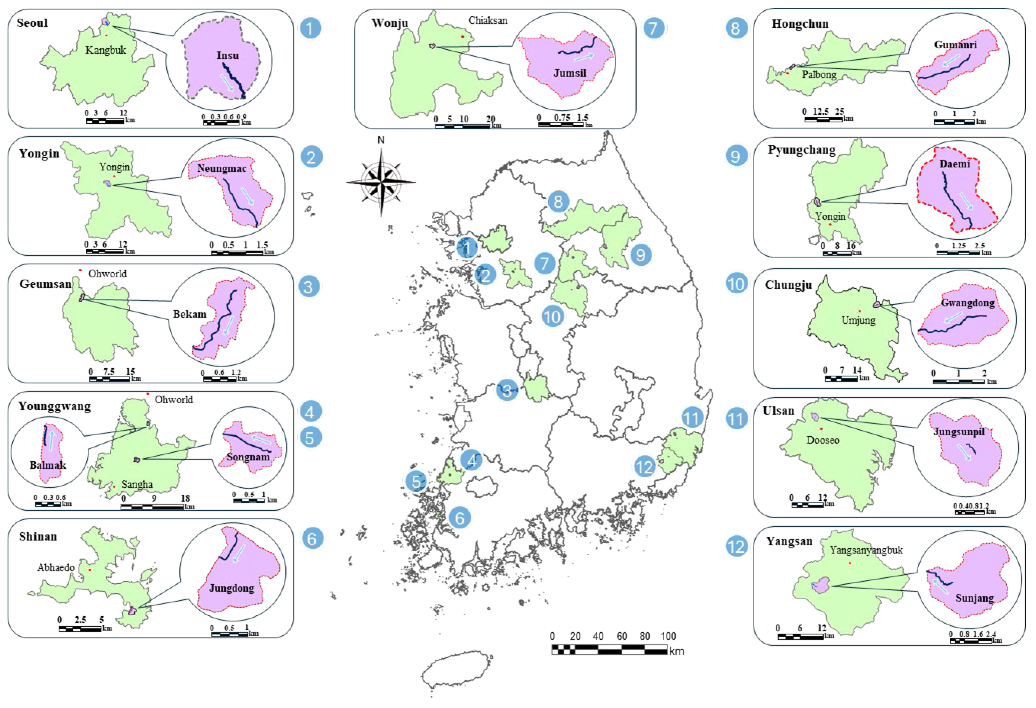
Figure 2.
Schematic diagram of the flood prediction framework for small streams.
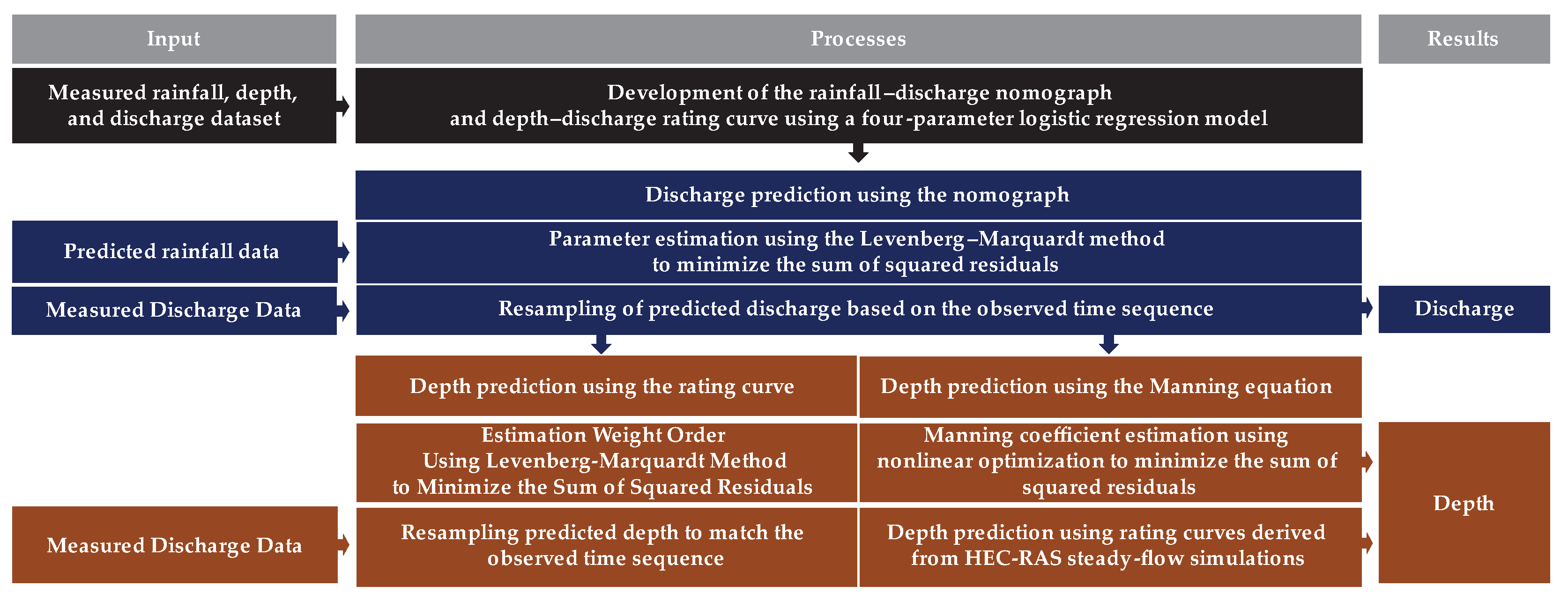
Figure 3.
Conceptual diagram of the iterative optimization process used to update the nomograph and rating curve and to estimate discharge and depth at gauged reaches.
Figure 3.
Conceptual diagram of the iterative optimization process used to update the nomograph and rating curve and to estimate discharge and depth at gauged reaches.
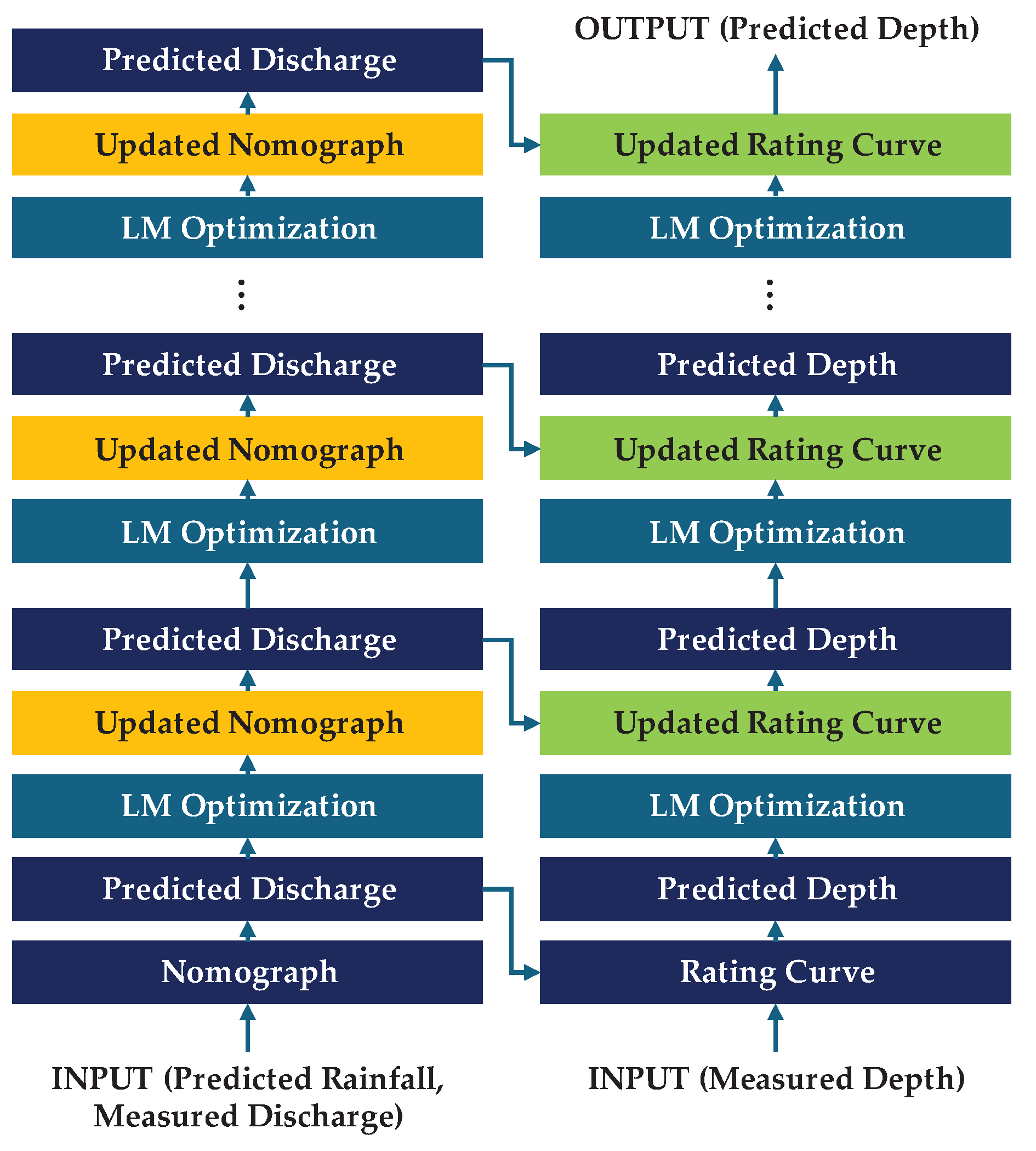
Figure 4.
Comparison of the twelve test-bed small-stream basins, including the number of surveyed cross-sections.
Figure 4.
Comparison of the twelve test-bed small-stream basins, including the number of surveyed cross-sections.
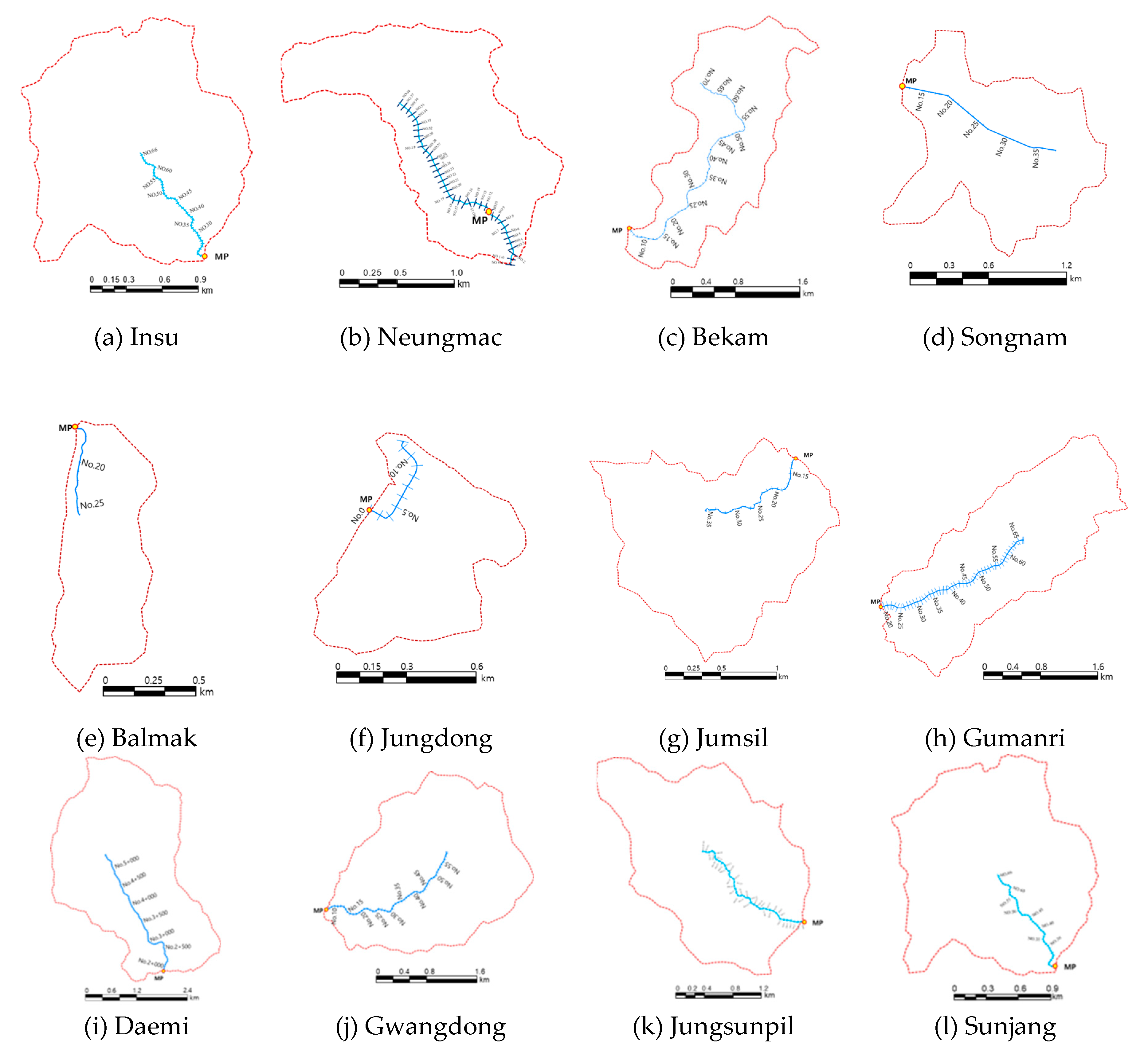
Figure 5.
Paired scatter plots for the twelve test-bed small streams: (a–l) each show (left) peak rainfall intensity versus peak discharge and (right) peak depth versus peak discharge, together with the fitted nonlinear 4PL regression curves.
Figure 5.
Paired scatter plots for the twelve test-bed small streams: (a–l) each show (left) peak rainfall intensity versus peak discharge and (right) peak depth versus peak discharge, together with the fitted nonlinear 4PL regression curves.
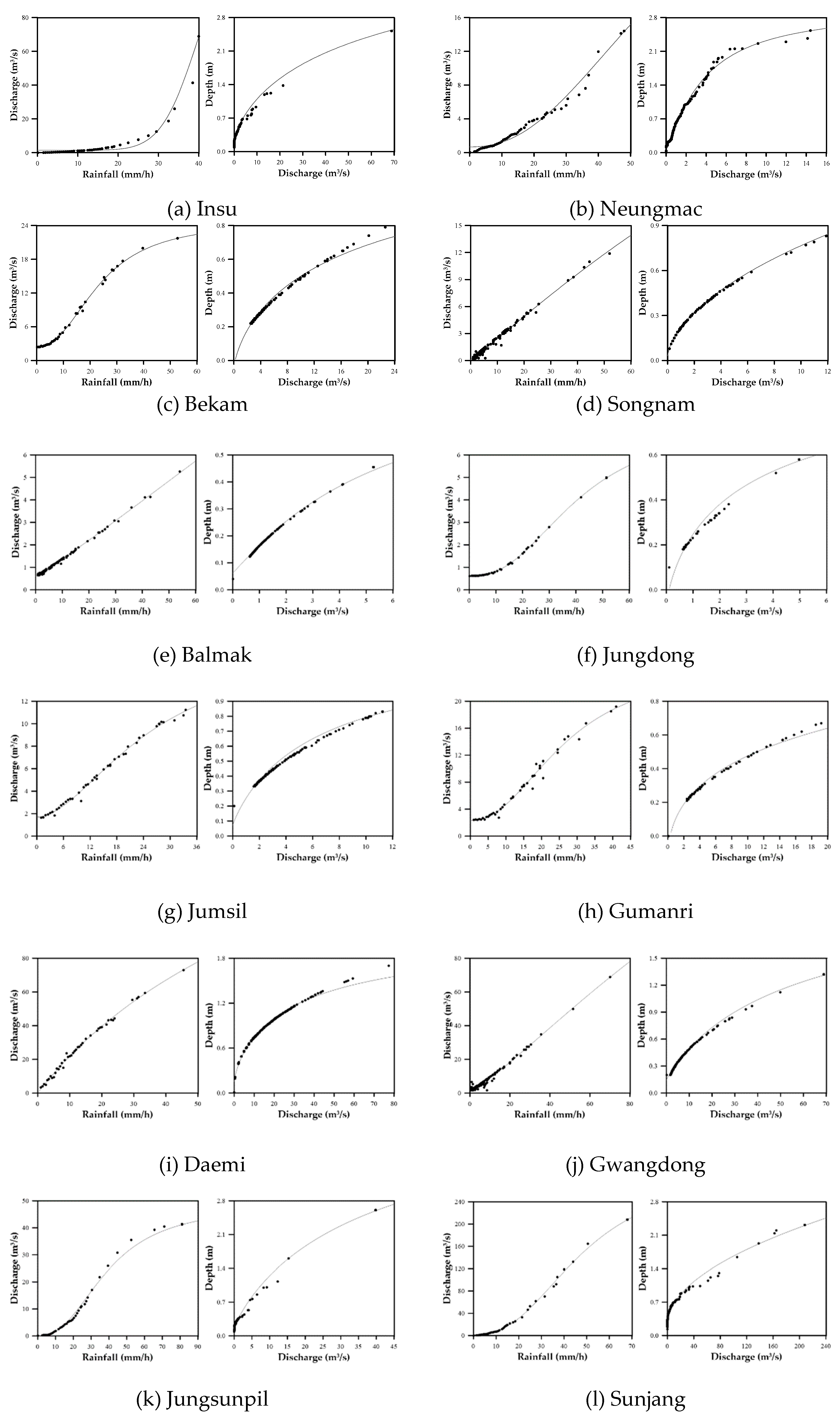
Figure 6.
Scatter plot of simulated peak water-surface elevation versus peak discharge for Jungdong stream, together with the fitted nonlinear 4PL regression curve.
Figure 6.
Scatter plot of simulated peak water-surface elevation versus peak discharge for Jungdong stream, together with the fitted nonlinear 4PL regression curve.
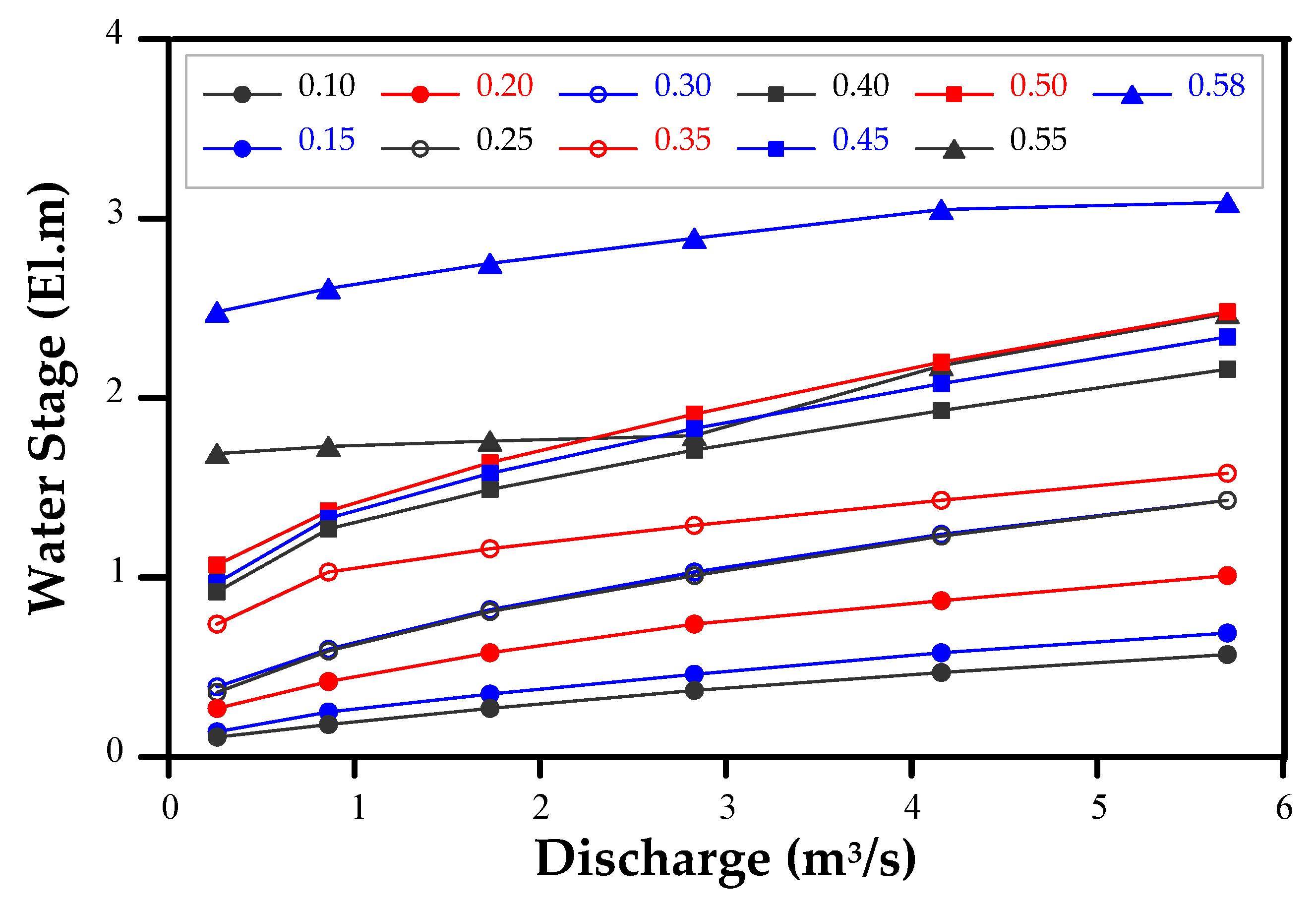
Figure 7.
Comparison of relative errors between predicted and measured rainfall by leading time.
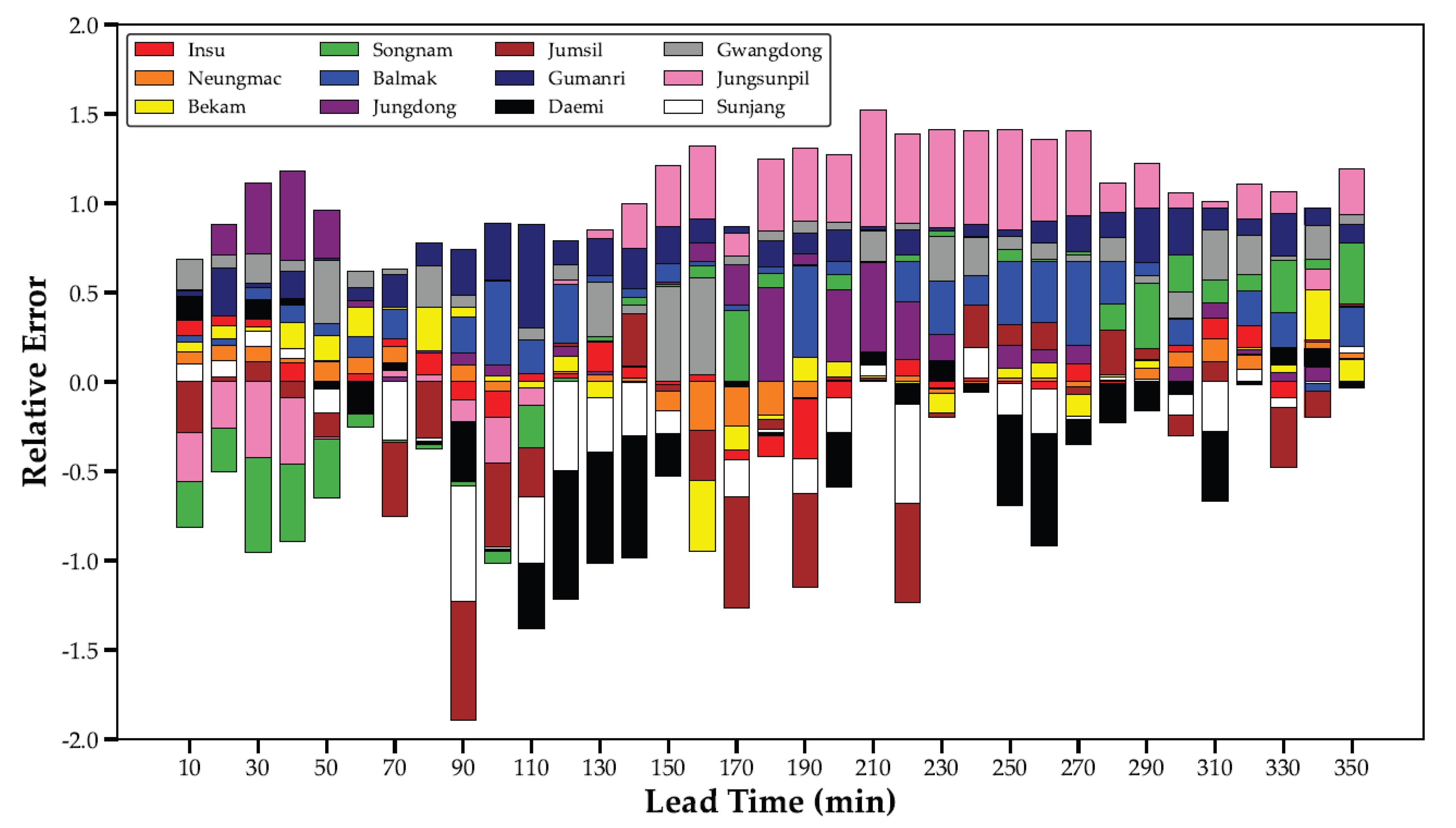
Figure 8.
Comparison between predicted and observed values for the twelve test-bed small streams: (a–l) each consist of two panels showing (left) discharge and (right) flood depth.
Figure 8.
Comparison between predicted and observed values for the twelve test-bed small streams: (a–l) each consist of two panels showing (left) discharge and (right) flood depth.
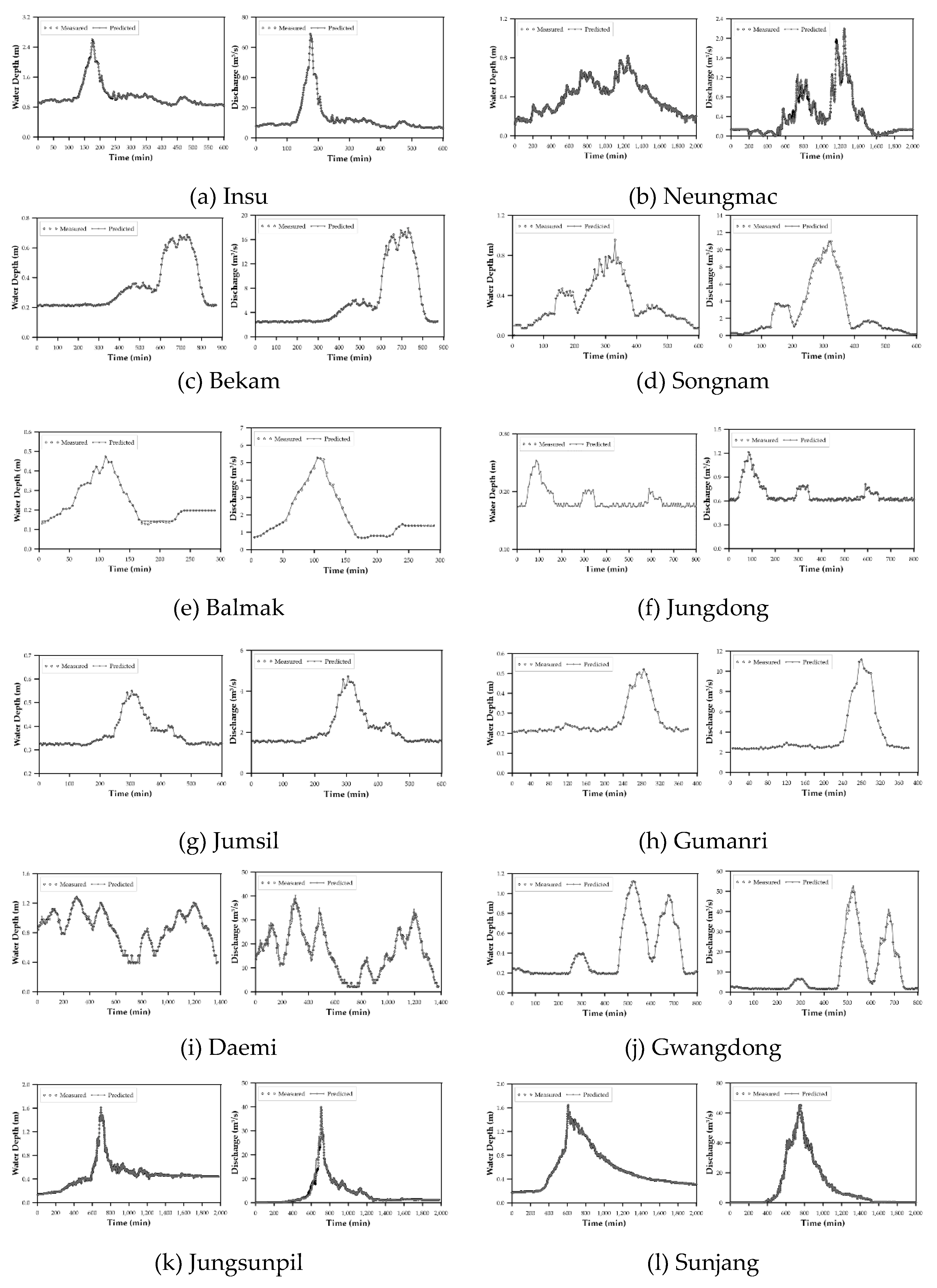
Figure 9.
Distribution of discrepancy ratios for discharge prediction at the twelve test-bed small streams.
Figure 9.
Distribution of discrepancy ratios for discharge prediction at the twelve test-bed small streams.
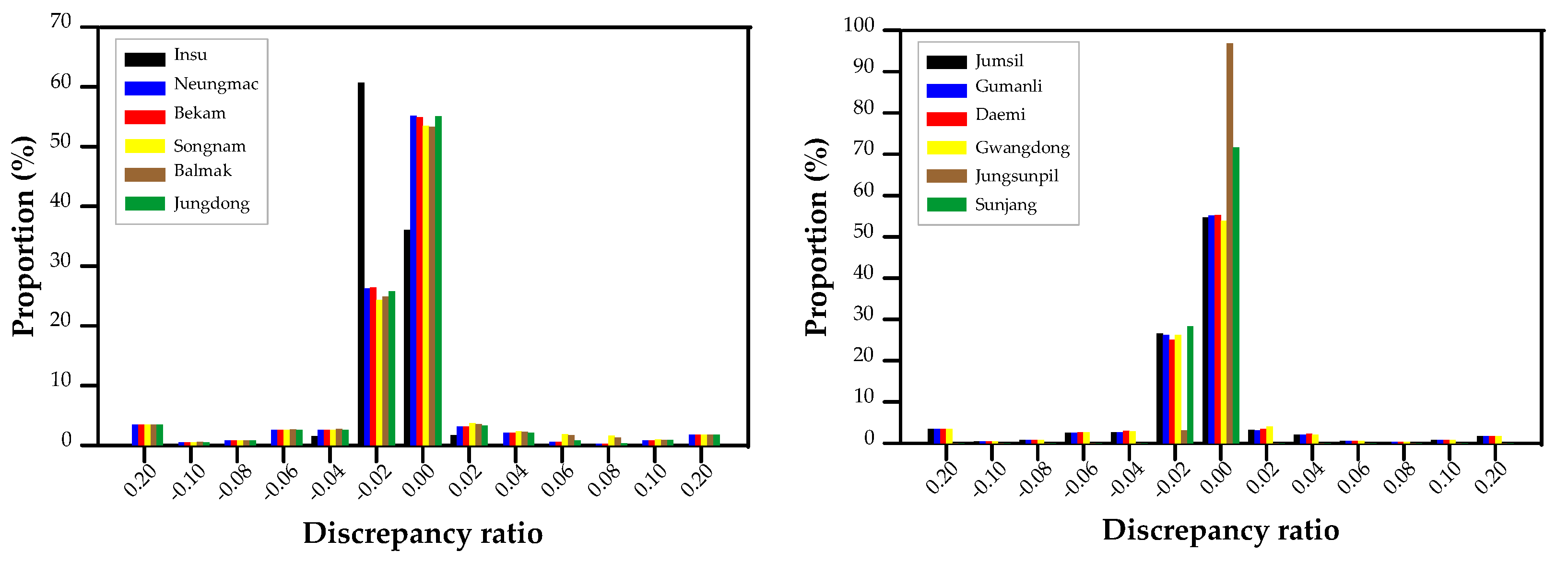
Figure 10.
Distribution of discrepancy ratios for water-depth prediction at the twelve test-bed small streams.
Figure 10.
Distribution of discrepancy ratios for water-depth prediction at the twelve test-bed small streams.
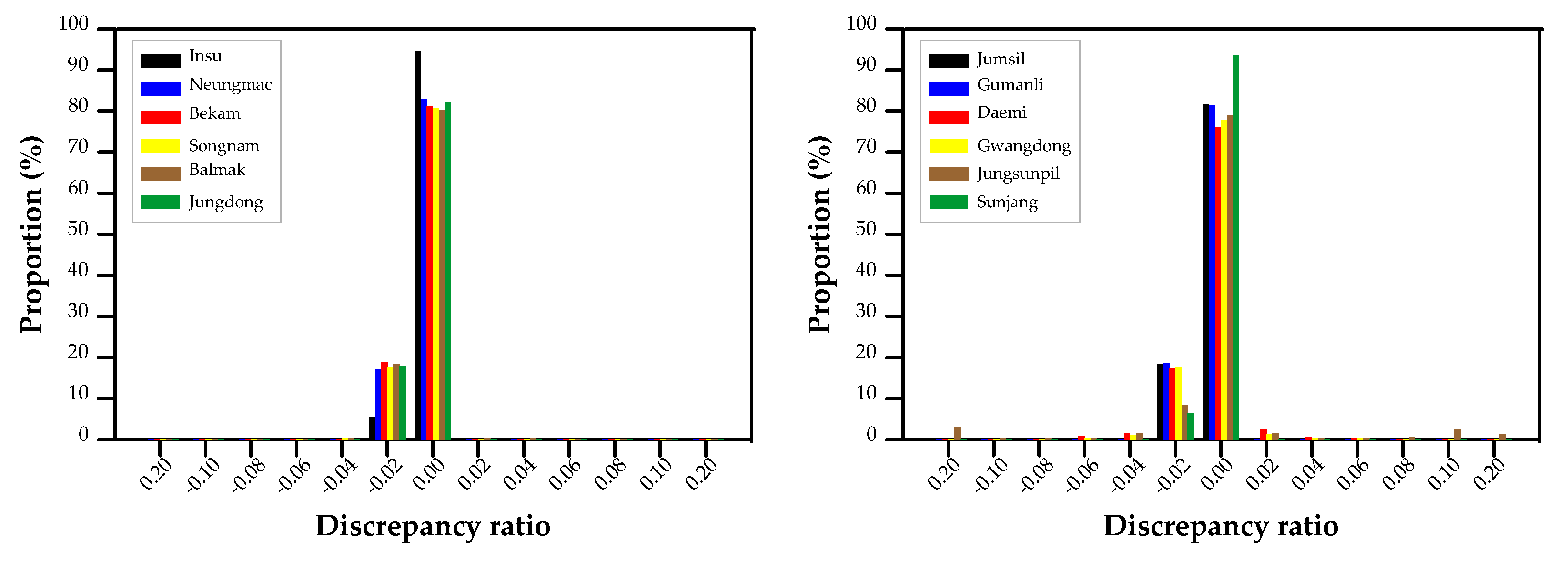
Figure 11.
Comparison of predicted flood depths in ungauged reaches obtained using the Manning equation and depth–discharge rating curves derived from HEC-RAS simulations.
Figure 11.
Comparison of predicted flood depths in ungauged reaches obtained using the Manning equation and depth–discharge rating curves derived from HEC-RAS simulations.
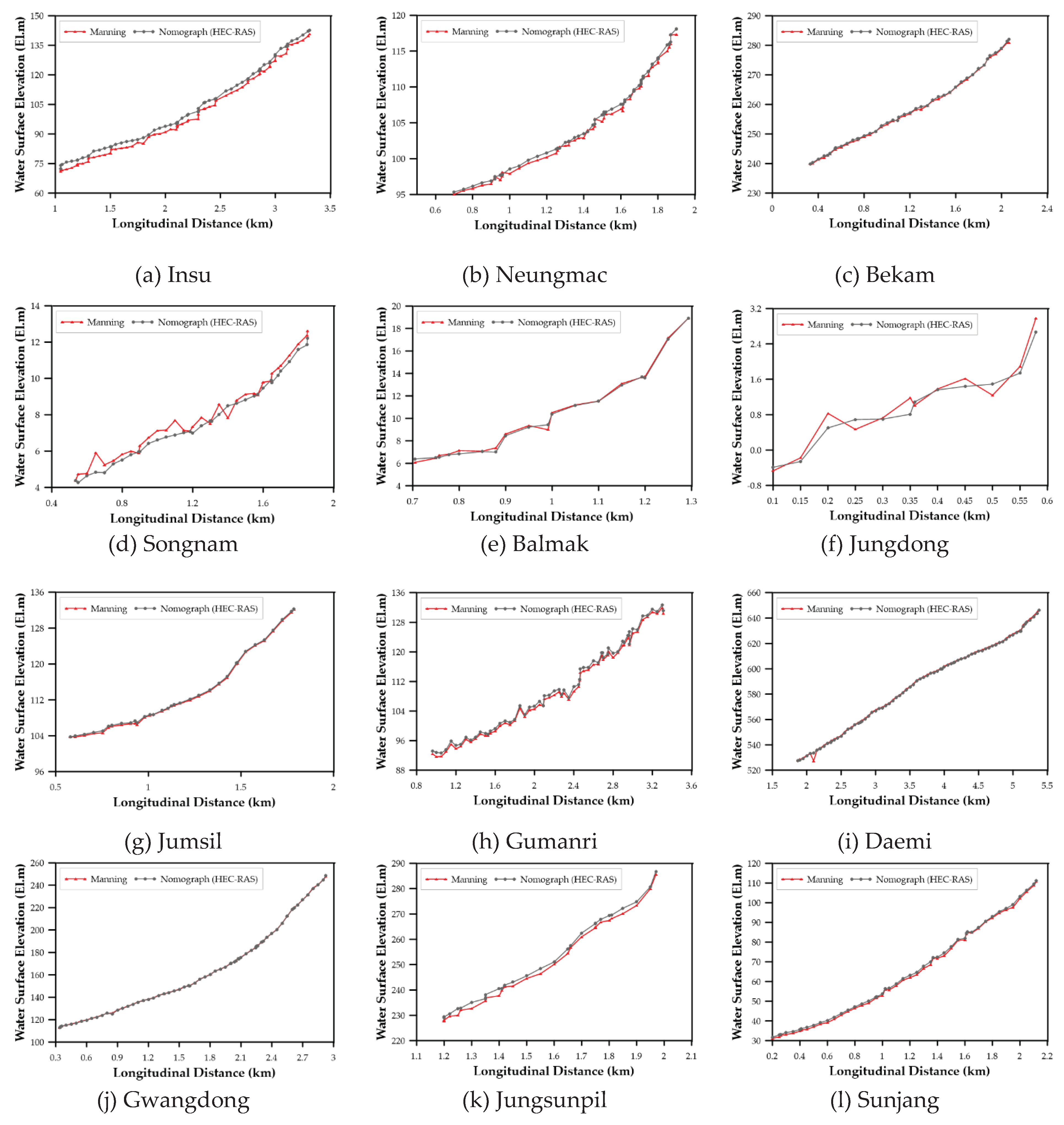
Figure 12.
Comparison between predicted water levels in ungauged reaches based on the Manning equation and levee-crest elevations.
Figure 12.
Comparison between predicted water levels in ungauged reaches based on the Manning equation and levee-crest elevations.
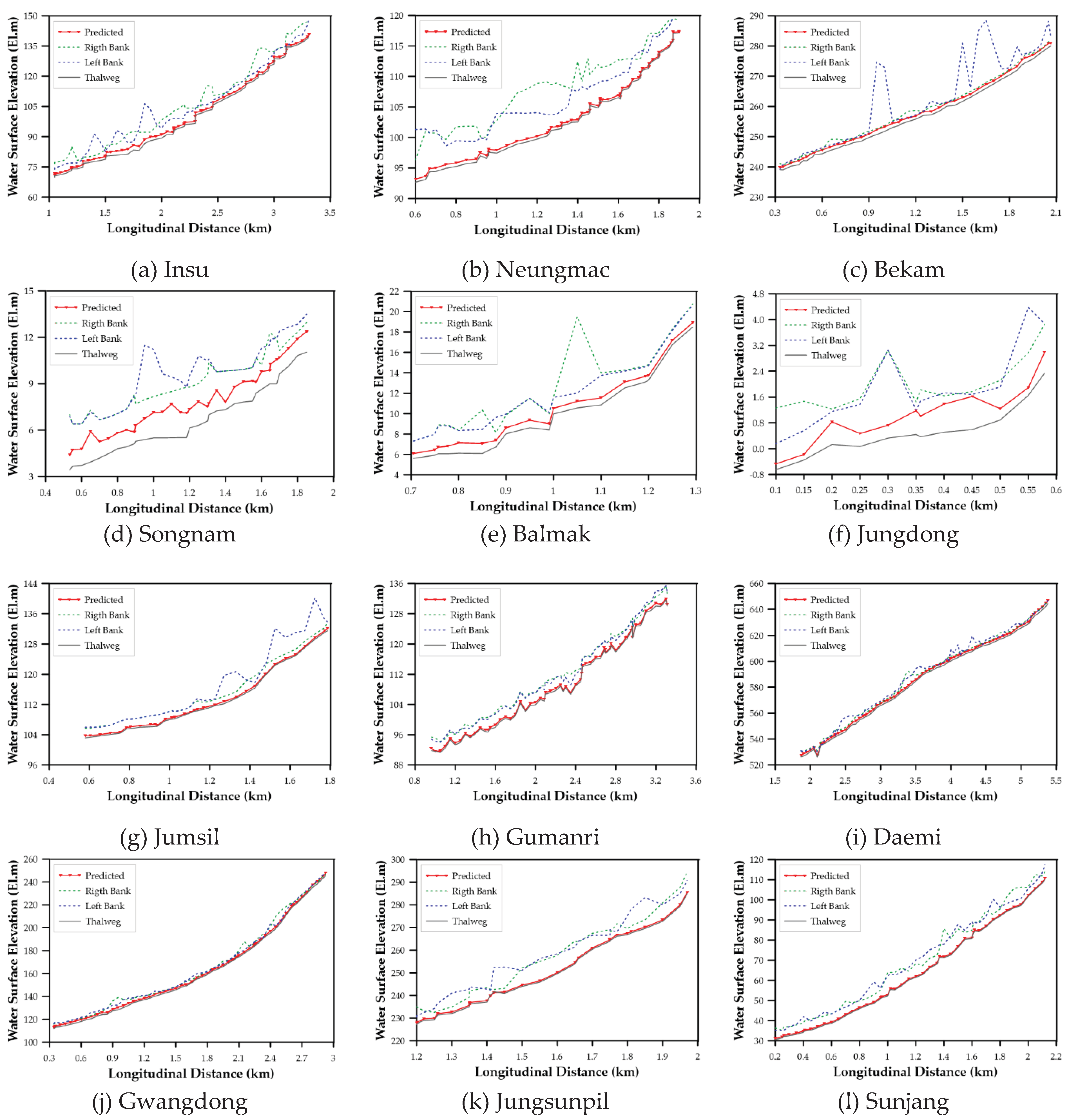

Table 1.
Basin and channel characteristics of the twelve test-bed small streams, together with SMMS and AWS information used for model development and evaluation.
Table 1.
Basin and channel characteristics of the twelve test-bed small streams, together with SMMS and AWS information used for model development and evaluation.
| Small Stream | SMMS | ) | (km) | (m) | ) | (El.m) | AWS | |||||
|---|---|---|---|---|---|---|---|---|---|---|---|---|
| Lat. | Lon. | Start Year |
Name | (km) | ||||||||
| Insu | 37.6671 | 127.0097 | 2020 | 3.66 | 3.12 | 17.1 | 0.025 | 0.040 | 71 | 140.8 | Uijungbu | 10.4 |
| Neungmac | 37.2418 | 127.1960 | 2018 | 2.41 | 3.09 | 9.45 | 0.054 | 0.035 | 30 | 119.0 | Yongin | 5.83 |
| Bekam | 36.1891 | 127.3887 | 2021 | 3.44 | 3.51 | 13.5 | 0.014 | 0.035 | 50 | 119.9 | Ohworld | 11.4 |
| Songnam | 35.2734 | 126.4482 | 2022 | 1.61 | 1.49 | 18.5 | 0.008 | 0.030 | 45 | 5.800 | Yeumsan | 10.1 |
| Balmak | 35.3703 | 126.4892 | 2022 | 0.59 | 0.53 | 6.80 | 0.028 | 0.035 | 14 | 7.700 | Sangha | 8.00 |
| Jungdong | 34.8337 | 126.3464 | 2023 | 0.50 | 0.60 | 15.0 | 0.004 | 0.030 | 13 | 17.30 | Abhaedo | 6.81 |
| Jumsil | 37.3914 | 127.9319 | 2021 | 2.59 | 1.29 | 12.6 | 0.019 | 0.030 | 57 | 105.1 | Chiaksan | 10.8 |
| Gumanri | 37.7204 | 127.7124 | 2022 | 5.00 | 2.69 | 24.0 | 0.026 | 0.035 | 108 | 86.47 | Palbong | 3.94 |
| Daemi | 37.4659 | 128.3205 | 2020 | 12.8 | 4.48 | 22.4 | 0.033 | 0.033 | 226 | 529.9 | Pyungchang | 11.8 |
| Gwangdong | 37.0919 | 127.9675 | 2022 | 6.36 | 2.95 | 11.6 | 0.048 | 0.030 | 96 | 105.8 | Umjung | 6.04 |
| Jungsunpil | 35.6558 | 129.1249 | 2016 | 5.09 | 3.18 | 14.0 | 0.096 | 0.033 | 181 | 287.3 | Dooseo | 4.23 |
| Sunjang | 35.4012 | 128.9303 | 2017 | 13.6 | 2.14 | 33.5 | 0.093 | 0.035 | 258 | 113.5 | Yangsan | 9.86 |
Table 2.
Mean and maximum observed rainfall, depth, and discharge for the twelve test-bed small streams.
Table 2.
Mean and maximum observed rainfall, depth, and discharge for the twelve test-bed small streams.
| Small Stream | Rainfall (mm/h) | Depth (m) | /s) | |||
|---|---|---|---|---|---|---|
| Mean | Max. | Mean | Max. | Mean | Max. | |
| Insu | 0.30 | 62.5 | 0.23 | 2.52 | 0.24 | 68.88 |
| Neungmac | 0.17 | 56.7 | 0.18 | 1.74 | 0.15 | 14.41 |
| Bekam | 4.80 | 53.5 | 0.26 | 0.79 | 3.66 | 22.60 |
| Songnam | 5.28 | 52.0 | 0.22 | 0.83 | 1.32 | 11.89 |
| Balmak | 5.60 | 54.0 | 0.16 | 0.46 | 1.03 | 5.270 |
| Jungdong | 5.79 | 51.5 | 0.20 | 0.58 | 0.80 | 4.980 |
| Jumsil | 5.87 | 33.5 | 0.42 | 0.83 | 2.93 | 11.25 |
| Gumanri | 5.52 | 41.0 | 0.26 | 0.67 | 3.87 | 19.20 |
| Daemi | 4.77 | 45.5 | 0.68 | 1.70 | 10.7 | 77.41 |
| Gwangdong | 5.34 | 70.0 | 0.33 | 1.32 | 5.76 | 68.94 |
| Jungsunpil | 0.16 | 80.0 | 0.24 | 1.98 | 0.83 | 35.93 |
| Sunjang | 0.19 | 95.8 | 0.40 | 2.45 | 1.32 | 210.3 |
Table 3.
Table 3. Optimal parameter estimates and coefficients of determination for the rainfall–discharge nomographs and depth–discharge rating curves obtained using nonlinear 4PL regression.
Table 3.
Table 3. Optimal parameter estimates and coefficients of determination for the rainfall–discharge nomographs and depth–discharge rating curves obtained using nonlinear 4PL regression.
| Small Stream | Rainfall-discharge Nomograph | Rainfall-discharge Nomograph | ||||||||
|---|---|---|---|---|---|---|---|---|---|---|
| Insu | 157.68 | 1.5100 | 41.492 | 7.6568 | 0.99 | 5.1104 | 0.2030 | 78.743 | 0.7266 | 0.99 |
| Neungmac | 39.417 | 0.6845 | 62.477 | 2.3113 | 0.99 | 3.0009 | 0.1162 | 3.8577 | 1.2360 | 0.99 |
| Bekam | 27.745 | 2.4519 | 23.573 | 2.3076 | 0.99 | 1.1325 | 0.0678 | 14.117 | 1.0735 | 0.99 |
| Songnam | 44.583 | 0.2286 | 118.98 | 1.2037 | 0.99 | 1.7342 | 0.0780 | 16.799 | 0.8224 | 0.99 |
| Balmak | 128.03 | 0.5922 | 1269.9 | 1.0451 | 0.99 | 1.5943 | 0.0353 | 17.225 | 0.8506 | 0.99 |
| Jungdong | 7.3403 | 0.6125 | 40.357 | 2.4766 | 0.99 | 1.9308 | 0.0720 | 15.396 | 0.8627 | 0.99 |
| Jumsil | 16.922 | 1.6994 | 25.577 | 1.8267 | 0.99 | 1.5999 | 0.1809 | 13.412 | 0.9977 | 0.99 |
| Gumanri | 25.609 | 2.3083 | 26.894 | 2.2040 | 0.99 | 1.0657 | 0.0211 | 13.057 | 0.8941 | 0.99 |
| Daemi | 185.00 | 1.4335 | 68.874 | 1.0803 | 0.99 | 2.2656 | 0.1526 | 33.238 | 0.7767 | 0.99 |
| Gwangdong | 299.25 | 1.9188 | 140.87 | 1.2460 | 0.99 | 3.0874 | 0.1047 | 115.68 | 0.7843 | 0.99 |
| Jungsunpil | 48.276 | 0.0012 | 39.327 | 2.4306 | 0.99 | 5.1949 | 0.1618 | 42.943 | 0.8858 | 0.99 |
| Sunjang | 296.39 | 1.5606 | 48.431 | 2.4886 | 0.99 | 178.80 | 0.2490 | 115290 | 0.5167 | 0.99 |
Table 4.
Optimal parameter estimates (, , , and ) and coefficients of determination for the depth–discharge rating curves derived for ungauged reaches of Jungdong stream, where is the length from downstream section.
Table 4.
Optimal parameter estimates (, , , and ) and coefficients of determination for the depth–discharge rating curves derived for ungauged reaches of Jungdong stream, where is the length from downstream section.
| (km) | |||||
|---|---|---|---|---|---|
| 0.100 | 1.6562 | 0.07675 | 12.679 | 0.98823 | 0.999 |
| 0.150 | 1.7492 | 0.10649 | 11.590 | 0.91619 | 0.998 |
| 0.200 | 2.0556 | 0.18570 | 7.5799 | 0.89316 | 0.998 |
| 0.250 | 3.6477 | 0.22136 | 12.230 | 0.81036 | 0.996 |
| 0.300 | 3.2137 | 0.28001 | 9.6464 | 0.86710 | 0.998 |
| 0.350 | 3.4521 | 0.35612 | 15.332 | 0.46564 | 0.995 |
| 0.400 | 4.0110 | 0.24921 | 6.1755 | 0.49375 | 0.993 |
| 0.450 | 7.5371 | 0.64369 | 43.344 | 0.57611 | 0.997 |
| 0.500 | 5.2424 | 0.96051 | 12.314 | 0.84141 | 0.998 |
| 0.550 | 5.1864 | 1.69520 | 9.4436 | 2.41860 | 0.987 |
| 0.579 | 3.5411 | 2.41650 | 3.5198 | 1.04710 | 0.994 |
Table 5.
Table 5. Prediction accuracy and root mean square error (RMSE) for discharge and flood depth at the twelve test-bed small streams.
Table 5.
Table 5. Prediction accuracy and root mean square error (RMSE) for discharge and flood depth at the twelve test-bed small streams.
| Small Stream | Rainfall (mm/h) | Depth (m) | ||
|---|---|---|---|---|
| Mean | Max. | Mean | Max. | |
| Insu | 100.0 | 100.0 | 0.0003 | 0.0080 |
| Neungmac | 93.20 | 77.41 | 0.0003 | 0.0336 |
| Bekam | 100.0 | 99.96 | 0.1924 | 0.0164 |
| Songnam | 77.45 | 76.79 | 0.1764 | 0.0089 |
| Balmak | 100.0 | 93.34 | 0.1071 | 0.0185 |
| Jungdong | 77.45 | 76.39 | 0.0482 | 0.0137 |
| Jumsil | 97.96 | 95.31 | 0.1147 | 0.0244 |
| Gumanri | 73.92 | 74.86 | 0.2715 | 0.0236 |
| Daemi | 97.96 | 85.15 | 1.1534 | 0.0518 |
| Gwangdong | 74.25 | 100.0 | 0.9340 | 0.0193 |
| Jungsunpil | 100.0 | 100.0 | 0.6306 | 0.0003 |
| Sunjang | 76.79 | 100.0 | 0.0004 | 0.0006 |
| Mean | 89.08 | 89.93 | 0.3024 | 0.0183 |
Disclaimer/Publisher’s Note: The statements, opinions and data contained in all publications are solely those of the individual author(s) and contributor(s) and not of MDPI and/or the editor(s). MDPI and/or the editor(s) disclaim responsibility for any injury to people or property resulting from any ideas, methods, instructions or products referred to in the content. |
© 2026 by the authors. Licensee MDPI, Basel, Switzerland. This article is an open access article distributed under the terms and conditions of the Creative Commons Attribution (CC BY) license (http://creativecommons.org/licenses/by/4.0/).
Copyright: This open access article is published under a Creative Commons CC BY 4.0 license, which permit the free download, distribution, and reuse, provided that the author and preprint are cited in any reuse.


