

Submitted:
20 March 2026
Posted:
23 March 2026
You are already at the latest version
Abstract
A phenomenological geometrical model is presented for the hyperfine structure of hydrogenic systems. The approach extends a previously published fine-structure analysis to hyperfine splittings by introducing a compact set of empirically constrained geometric corrections. Unlike conventional quantum electrodynamic treatments which reference the Lamb shift to the hyperfine centroid, the present framework targets the hyperfine mid-point, corresponding to a substantially larger reference interval. Despite this difference in reference scale, agreement with experimental hyperfine and Lamb-shift-related data at the 0.01 MHz level is obtained across multiple hydrogen states. The model is further extended to deuterium, tritium, 3He+, and 7Li2+, revealing systematic cross-nuclear behaviour and a universal scaling relation involving nuclear mass number and charge. The calculations employ a simplified geometric scheme that does not rely on perturbative quantum electrodynamics but is intended as a complementary phenomenological description. Possible physical interpretations in terms of structured internal dynamics are discussed, together with limitations and directions for further development.
Keywords:
photonics
; SAM
; OAM
; photonic
; toroidal
; vortex
; hydrogen
; atom
; hyperfine
; structure
1. Introduction
1.1. Preliminary
Atomic hyperfine structure is conventionally described within quantum electrodynamics (QED) using perturbative expansions that incorporate relativistic, radiative, and nuclear effects. These calculations have achieved remarkable quantitative success but often involve substantial computational complexity and limited geometrical transparency. This has motivated the exploration of alternative representations that aim to capture observed regularities using reduced or explicitly structured formalisms [1,2,3,4].
The present work extends a previously published phenomenological geometrical framework, originally applied to fine structure phenomena, to the hyperfine structure of hydrogenic systems [4]. Within this framework, atomic energy shifts are represented using structured internal degrees of freedom that admit a geometrical interpretation. The model is not derived from perturbative QED, nor is it intended to replace it; rather, it offers a complementary phenomenological description in which mass, electric potential, magnetic fields, and electromagnetic induction are represented within geometric and rotational structure.
A distinctive feature of the model is its focus on the hyperfine mid-point rather than the hyperfine centroid traditionally used in Lamb-shift calculations. This choice leads to a substantially greater reference frequency interval but allows the hyperfine splitting to be interpreted in terms of geometric field coupling between electronic and nuclear rotational modes. This newly-defined Lamb shift requires two empirically consistent corrections to the fine structure formula: a relative-to-proton speed adjustment, and a magnetic potential adjustment. Within the PTV framework, the magnetic potential adjustment is not treated as a static interaction evaluated at the bound-state radius, but as the accumulated effect of the proton’s magnetic momentum field acting on the electron Sp-2 circuit as the electron is transported , within the model, from infinity to the bound-state separation. This interpretation parallels the cumulative Sp-3 interaction associated with bound-state formation.
The corrections employ four adjustable parameters, each associated with a specific physical or geometrical role.
The parameters and —Equations (13) and (22)—participate in the relative-to-proton speed adjustment and magnetic potential adjustment, respectively, while in Equation (22) is suggestive of a magnetic dipole-dipole interaction for all hydrogen and deuterium states. A fourth parameter from Table 7 in Equation (35) governs the hyperfine shift and varies across angular momentum states. The parameter constraints are as follows. The and are connected through a universal scaling law that holds for hydrogen deuterium, tritium, 3He+, and 7Li2+ in Equation (37), while is consistent across all hydrogenic states examined (Table 2 and Table 5, Table 6 and Table 7). For states, corresponds to the absence of any hyperfine adjustment and reinforces the Sp-2 parallel field assumption for magnetic interactions. Deviations from this value for other states may be interpreted geometrically in terms of reduced proton field coupling arising from increased electronic eccentricity.
These features substantially reduce parameter freedom and distinguish the model from unconstrained empirical fitting. With the laboratory creation of photonic toroidal vortex states [5], precision OAM experiments provide a suggestive analogy for the structured elements employed in the model.
1.2. History and Background
Experiments on electron vortices in transmission electron microscopes have shown that electrons can occupy quantized orbital states with large orbital angular momentum (OAM), even in free space, without a confining potential or external field [6,7,8]. This disassociation of quantized angular momentum from an external potential motivates the exploration of alternative representations alongside models such as Darwin’s relativistic derivation of the hydrogen fine structure from Dirac’s equation [9,10]. By combining Sommerfeld’s classical treatment [11,12] with recent optical OAM experiments [13], a Photonic Toroidal Vortex (PTV) phenomenological model has been proposed in which the electron structure is represented using a toroidal geometric structure [4]. When this representation is applied in the presence of a corresponding proton structure, charge effects occur and fine-structure energies can be reproduced with high accuracy [4]. The present work introduces an effective representation of the observable electron rest mass in terms of a pure optical OAM, see Section 1.3.2. This geometrical model is then employed to estimate the Lamb shift and the hyperfine splitting of the hydrogen atom. An extension to deuterium, using the single-PTV hydrogen nucleus as an approximation, yields agreement at the level of 22 parts in one billion.
Interest in the hyperfine levels can be traced back to Lamb and Retherford’s discovery that the energy differs from the by MHz [14]. This violates Dirac’s prediction. Quantum electrodynamics (QED) has produced successive corrections [15,16,17], establishing the Lamb shift as the difference between the Sommerfeld–Dirac fine-structure energy and the experimental centroid of the hyperfine manifold. Here, the centroid arises from the mean of the hyperfine frequencies weighted according to transition amplitudes.
The standard relativistic and QED reference equations can be summarized as follows. Together they define the conventional hyperfine baseline against which the PTV modifications are applied. For an electron moving in the Coulomb field of a point nucleus, the frequency (MHz) is approximated by
Here, is the nuclear charge, is the Rydberg constant, is the principal quantum number, is the angular momentum quantum number, , and , see Table A1, Appendix A.1
The relativistic reduced mass correction (MHz) is
where and are the electron and proton rest masses, respectively.
For example, to calculate the Lamb shift for the state of atomic hydrogen, we set , , , and take the experimentally observed hyperfine centroid MHz ([18], Table 4). The observed Lamb shift is then
The first two terms on the right of Equation (3) produce a magnitude of MHz with the result that the hydrogen state shifts by MHz.
The hyperfine splitting about the centroid, arising from magnetic dipole-dipole coupling between the electron and proton spins, is given in atomic units from Ref. ([19], p.240), see Table A1, Appendix A:
where
For example, for the ground state of hydrogen, the quantum numbers are nuclear spin , total quantum number , total electron angular momentum , and electron orbital angular momentum which leaves
Here, the total atomic angular momentum quantum number takes the values . This gives MHz and MHz. Figure 1 shows the shifts relative to the reduced mass adjusted fine-structure value, see Equation (3).
1.3. Assumptions of the PTV Model
In the specific realization adopted here, the structured internal degrees of freedom are represented by a Photonic Toroidal Vortex (PTV) model. The assumptions of the PTV model that are relevant to the present work are as follows ([4], Figure 3).
1.3.1. The Helical String (Sp-1 Rotation)
1.3.2. Optical OAM (Sp-2 Rotation)
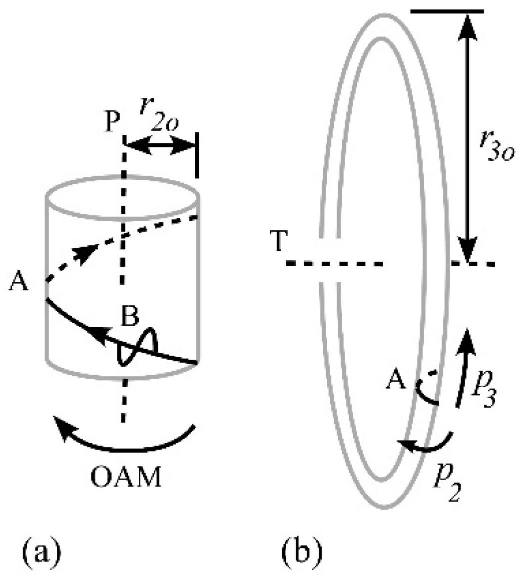
The string is then wrapped around a notional tube to form a Sp-2 rotation, see Figure 3a. A closed trajectory constitutes the Sp-2 rest mass ([4], Equation (1)) and this is the electron rest mass presented in Table A1 or, on a smaller scale, the proton rest mass .
Figure 3.
Construction of a PTV. a A helical string B from Figure 2a circulates in a helical trajectory around an axis P as optical OAM on a notional tube A. This also has linear momentum parallel to axis P. b The notional tube A is given a curved trajectory about an axis T on a notional toroid. Here, P is the poloidal axis and T is the toroidal axis of the PTV. The magnetic and electric momenta are and , respectively.
Figure 3.
Construction of a PTV. a A helical string B from Figure 2a circulates in a helical trajectory around an axis P as optical OAM on a notional tube A. This also has linear momentum parallel to axis P. b The notional tube A is given a curved trajectory about an axis T on a notional toroid. Here, P is the poloidal axis and T is the toroidal axis of the PTV. The magnetic and electric momenta are and , respectively.
1.3.3. PTV Construction (Sp-3 Rotation)
The trajectory of the Sp-2 tube axis is subsequently curved into a toroidal path to form the complete Photonic Toroidal Vortex (PTV), characterized by poloidal rotation (Sp-2) and toroidal rotation (Sp-3), see Figure 3b. The Sp-3 rotation constitutes an internal self-potential that plays the role of the external potential required in the Dirac–Sommerfeld scheme to produce results. The resulting bound-state geometry in the PTV model leads to the discrete fine-structure and, as shown in the present paper, also hyperfine-structure frequencies without invoking radiative-correction series. Without radiation absorption (unloaded case [4], Section 2) the Sp-2 mass becomes relativistic with Sp-3 speed . This speed is reduced as oppositely-rotating radiation is absorbed (loaded case [4], Section 3) and the toroids adopt higher energy levels. The ‘higher’ the energy level the smaller is the Sp-3 rotation frequency, [4], Section 3.1.3
The provision of Sp-3 speed to the electron rest mass gives it a raised relativistic mass in the toroid which in ground state is given by ([4], Equation (10)) the following:4
Within the PTV framework, electric charge is associated with Sp-3 rotation, so that free electrons are treated as necessarily Sp-3 structured. Accordingly, within the PTV model, free electrons in metals, cathode rays, and beta rays are all Sp-3 rotations. This differs from the classical Bohr picture in which a free electron is taken to adopt a rotating orbit.
The poloidal and the toroidal momenta are orthogonal, giving rise to the magnetic () and electric () momentum components. These rotations continuously generate momentum fields, though their detailed propagation characteristics are represented by the parallel field approximation in Section 1.3.5.
1.3.4. PTV Energy
The Sp-2 and Sp-3 energies of rotation are calculated from the following, respectively ([4], Equations (4) and (48)):
where momentum and velocity have adopted the rotation-type subscripts 2 and 3.
1.3.5. The Momentum Field
Figure 4.
A schematic representation of the proton momentum field components (not to scale). a The proton field source (left) generates an electric momentum field (dots/crosses) that can penetrate a target PTV (right). The field and resident momenta in the target rotate in opposition as an attraction interaction. b The proton also generates a magnetic momentum field . In the parallel field approximation, these vectors are treated as approximately parallel in the locality of the target Sp-2 circuit.
Figure 4.
A schematic representation of the proton momentum field components (not to scale). a The proton field source (left) generates an electric momentum field (dots/crosses) that can penetrate a target PTV (right). The field and resident momenta in the target rotate in opposition as an attraction interaction. b The proton also generates a magnetic momentum field . In the parallel field approximation, these vectors are treated as approximately parallel in the locality of the target Sp-2 circuit.
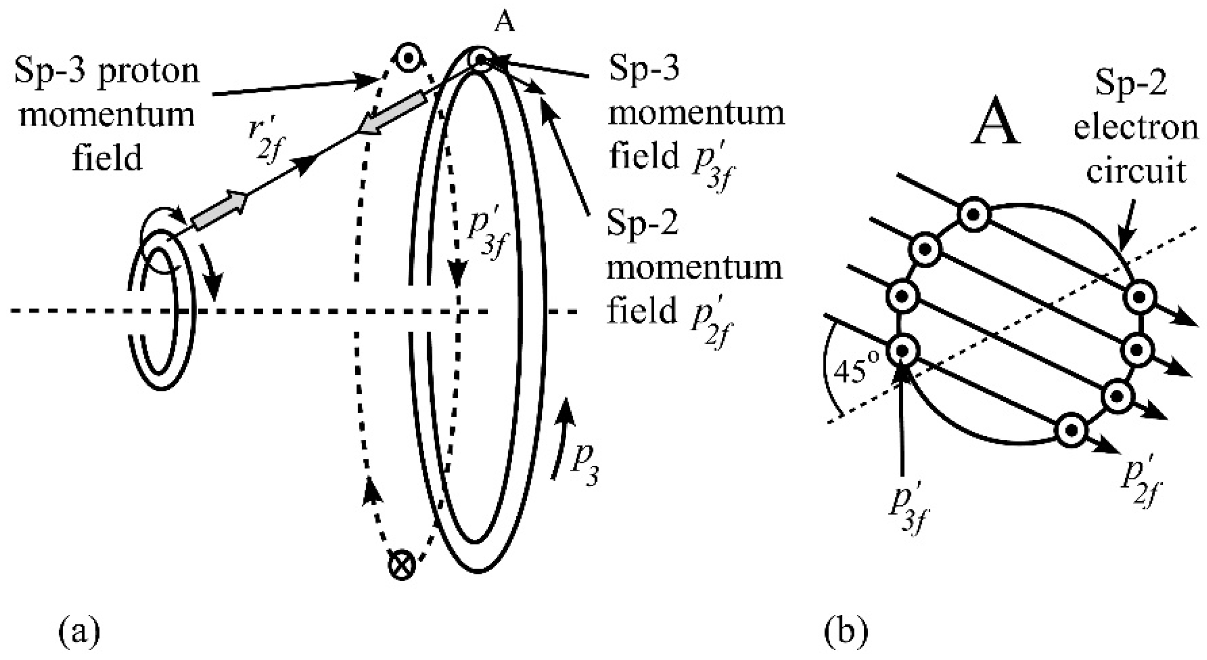
The PTV model proposes that both Sp-2 (poloidal) and Sp-3 (toroidal) rotations generate momentum fields in the surrounding space, though the complete dynamics of the field are not fully specified in Ref. [4]. As the PTV rotates, momentum field emissions occur continuously from the curvature of the Sp-1 helical trajectory in both Sp-2 and Sp-3 motion. The electron’s Sp-2 magnetic momentum field and its Sp-3 electric momentum field are mutually perpendicular components of the total momentum field. Following the approach in Ref. ([4], Equations (25), (26), (45) and (46)) in which we allow the field speed to diminish with while the field mass remains invariant, and for the electron we adopt the field momentum magnitudes:5
where is the field radius from the Sp-2 center, is the fine structure constant, and .6 For the proton, . From Equation (9), the field components maintain their relationship as they propagate through space:
The continuous generation of field emissions is formally unbound within the model though only a portion of field that interacts with the Sp-2 rotational geometry becomes accessible. The field otherwise remains undetected.
We now consider the parallel field approximation. The spiral field geometry in Ref. ([4], Figure 11) suggests that the proton magnetic momentum field vectors actually arrive at to the line joining the proton-electron Sp-2 centers due to the field emission mechanism.7 Here, the field momentum is to be given two degrees of freedom in the plane perpendicular to the proton’s poloidal axis: radial and azimuthal (Sp-2 rotational) momentum. We assume equal partitioning between these components such that each carries magnitude . Only the Sp-2 azimuthal component of the field participates in the magnetic coupling. A pure radial field and a pure azimuthal field would both produce a zero line integral around a circuit. In the parallel field approximation, the field orientation remains constant at the two points where any radial line from the proton center intersects the electron circuit. This eliminates the geometric compensation present in pure azimuthal fields, where two different alignment angles on this radial line exactly cancel the 1/r magnitude variation. With constant field orientation—see in Equation (27)—only the magnitude varies, producing a net non-zero line integral proportional to the integrated field strength around the electron Sp-2 circuit. As we shall in Section 3.4, the ratio between radial and azimuthal momentum may represent a fundamental constraint on field geometries capable of generating magnetic coupling. This non-cancelling geometry is essential: without the radial momentum component that straightens the spiral and enables the parallel field approximation, the line integral would vanish as it does for purely radial and purely azimuthal fields.
2. Methodology
2.1. PTV Calculations
The calculation obtains the Sp-3 rotation frequencies of the electron toroid. Transition frequencies are the differences between them. An emission results from the transition from a low frequency level (high ) to a high frequency state (low ) emitting a circularly polarized or optical OAM ray that rotates in opposition to the Sp-3 rotation. The unadjusted fine structure is calculated from (Ref. [4], Equation (51)) with a conversion from energy (J) to frequency (MHz).
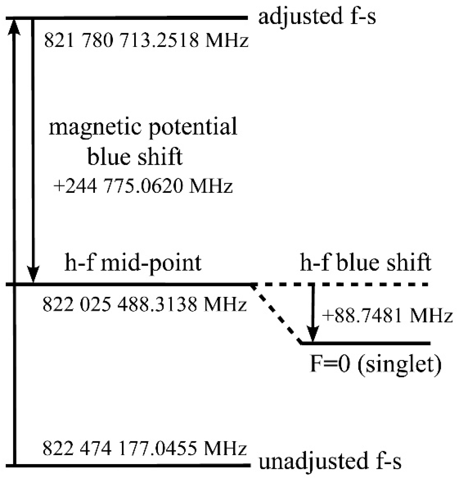
The center of mass is located on the rotating line joining the centers of the proton and electron Sp-2 circuits and is transformed to the proton rest-mass frame so that the speed of the electron relative to the proton is obtained, see Section 3.2. The consequent frequency obtained is , see Equations (12) and (13). This is the adjusted fine structure frequency indicated in Figure 5 and Figure 6. The mechanism for this depends on the relative proton–electron Sp-2 rotation senses. There are two cases that are set out in Table 1: (a) the proton–electron Sp-2 have the same sense so that a reduction is imposed on the proton Sp-2 frequency (); or (b) they are opposite sense in which case an increase is imposed (). For (a), the result is an extraction of action from the proton Sp-3 rotation to restore the Sp-2 action, so that the proton advances towards the electron, see Equation (13). With (b), the extra Sp-2 action is displaced into the proton Sp-3 and so it retreats from the electron, see Equation (13).8 However, there is also a red shift or blue shift that needs to be accounted for that targets the hyperfine midpoint frequency, in which the and are empirically determined constants, see Equation (22) with Table 2 and Table 3. This is the ‘magnetic potential adjustment’ calculation in Section 3.3. While the traditional Lamb shift calculation aims for the centroid for the hyperfine states, the PTV method targets the mid-point of the two values in the absence of an external field. So, the magnetic potential in Equation (22) is analogous to the Lamb shift calculation and is shown in Figure 5 and Figure 6.
Comparison of the traditional Lamb shift frequency in Figure 1 with the PTV magnetic potential shifts in Figure 5 and Figure 6 shows that the PTV shift to be accounted for is far greater. The hyperfine shift also depends on the relative rotation senses of the proton-electron Sp-2 circuits, in which the electron Sp-2 energy is raised or lowered by the same frequency about the hyperfine mid-point, see Equation (35). However, there is an assumption that is vital to the hyperfine calculation. While the proton Sp-2 field is generated continuously as the proton structure rotates, we assume that in the locality of the electron Sp-2 circuit, the field momentum vectors are approximately parallel, at to the line joining the Sp-2 centers, and lying in the plane of the electron Sp-2 circuit, see Figure 4b. The parallel-field approximation is validated by the requirement from Table 7 for the states in Equation (35) as this represents no adjustment.
The raising or lowering of the hyperfine mid-point occurs because the motion of the electron towards the proton results in a change in the proton’s Sp-2 momentum field integrated around the electron Sp-2 circuit. This energy is redistributed into Sp-3 motion. In summary, the full calculation for the pair of hyperfine frequencies is as follows, see also Equation (50):
Here, and and are both negative for (see Figure 5), and both positive when (see Figure 6). The shifts applied to the adjusted fine structure are given by Equations (12) and (13) and are summarized in Table 1.
Figure 5.
The state of hydrogen calculated from the PTV model with , see Appendix B. The unadjusted fine structure frequency (MHz) with no reduced mass is shown from Ref. ([4], Equation (51)). The adjusted fine structure frequency , including the state-dependent reduced mass and proton-speed correction, is shown from Equations (12) and (13). The ‘magnetic potential’ red shift is calculated from Equation (22) and Table 2 to reach the hyperfine mid-point. The hyperfine shift from the mid-point is calculated from Equation (35).
Figure 5.
The state of hydrogen calculated from the PTV model with , see Appendix B. The unadjusted fine structure frequency (MHz) with no reduced mass is shown from Ref. ([4], Equation (51)). The adjusted fine structure frequency , including the state-dependent reduced mass and proton-speed correction, is shown from Equations (12) and (13). The ‘magnetic potential’ red shift is calculated from Equation (22) and Table 2 to reach the hyperfine mid-point. The hyperfine shift from the mid-point is calculated from Equation (35).
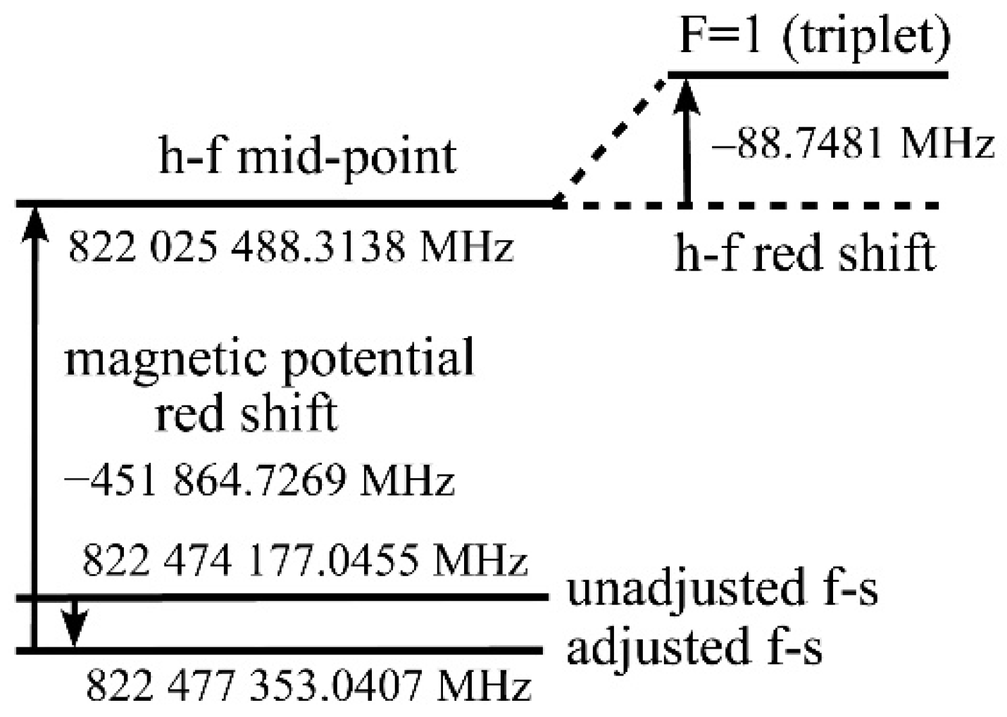
Figure 6.
The state of hydrogen calculated from the PTV model with . The unadjusted fine structure frequency (MHz) with no reduced mass is shown from Ref. ([4], Equation (51)). The adjusted fine structure frequency , including the state-dependent reduced mass and proton-speed correction, is shown from Equations (12) and (13). The ‘magnetic potential’ blue shift is calculated from Equation (22) and Table 3 to reach the hyperfine mid-point. The hyperfine shift from the mid-point is calculated from Equation (35).
Figure 6.
The state of hydrogen calculated from the PTV model with . The unadjusted fine structure frequency (MHz) with no reduced mass is shown from Ref. ([4], Equation (51)). The adjusted fine structure frequency , including the state-dependent reduced mass and proton-speed correction, is shown from Equations (12) and (13). The ‘magnetic potential’ blue shift is calculated from Equation (22) and Table 3 to reach the hyperfine mid-point. The hyperfine shift from the mid-point is calculated from Equation (35).
From Table 2 and Table 3, the value and sign of in Equation (22) turns out to be related to that of —see Section 3.2 and Equation (37). So with across all states, Equation (22) has the character of a magnetic dipole-dipole interaction. So we shall refer to Equation (22) as a ‘magnetic potential adjustment’ that results from the interaction of the proton Sp-2 field on the electron, one that is in need of further investigation. In fact, the connection between and extends also to deuterium (Table 11 and Table 12), tritium (Table 15), and 3He+ (Table 16) which leads to our proposal of a universal nuclear scaling law in Equation (37).
The full calculation for the state with appears in Appendix B with the results represented in Figure 5.

Table 1.
rotation senses determine the sign of in Equation (13), the effect on the proton motion in the center of mass frame, the electron fine structure energy in Equation (12), the hyperfine shift in Equation (35), and the magnetic potential shift in Equation (22).
Table 1.
rotation senses determine the sign of in Equation (13), the effect on the proton motion in the center of mass frame, the electron fine structure energy in Equation (12), the hyperfine shift in Equation (35), and the magnetic potential shift in Equation (22).
| relative Sp-2 senses | sign | proton motion | hyperfine shift | mag. pot. shift | |
|---|---|---|---|---|---|
| same | towards electron | increases | red | red | |
| opposite | away from electron | decreases | blue | blue |
2.2. Comparison with QED
The PTV approach trades mathematical accuracy for conceptual clarity. While the -function—Equation (13)—and the multipliers—Table 7 and Equation (35)—are empirically determined, they are consequences of a geometrical model. The magnetic potential—Table 2 and Table 3 with Equation (22)—needs further investigation but it results from the effect of the proton Sp-2 momentum field on the electron Sp-2 circuit. PTV theory provides a calculation that uses the same equations for each combination. These calculations can be performed on an electronic calculator across 30 pairs of hyperfine frequencies for each of the two signs of featuring the first six states for each of ,, , , and , see Appendix B.
PTV calculation ([4], Equation (51))
- (1)
- Modified fine structure equation, Equations (12) and (13)
- (2)
- (3)
- State-dependent reduced mass correction, Equation (13)
- (4)
- Relative-to-proton speed adjustment, Equations (12) and (13)
- (5)
- (6)
- Hyperfine shift, Equation (35)
- (1)
- Dirac equation solution
- (2)
- Self-energy correction (multi-loop integrals)
- (3)
- Uehling potential shift
- (4)
- Wichmann-Kroll corrections
- (5)
- Higher-order radiative corrections in
- (6)
- Nuclear size corrections to the Dirac energy
- (7)
- Relativistic recoil correction
- (8)
- Relativistic reduced mass correction
Considering mean absolute errors, QED’s hyperfine splitting accuracy is times more accurate than PTV, however, the PTV median is only 0.0015 MHz against the QED median of MHz based on 16 states, see Table 10. The PTV’s Lamb shift accuracy is times more accurate than QED, see Table 15. However, they are not accounting for the same frequency difference, the PTV difference being times the QED difference for the state. Since PTV uses the same basic equations for each state, its computational task represents a 10-fold reduction in complexity. The comparative errors are given in Section 4.
3. Hydrogen PTV
3.1. Fine Structure Corrections
Analogous to the Lamb shift calculations in QED, there are also correction terms for the PTV model: the proton speed adjustment, and the magnetic potential adjustment. These are both empirical formulae and unlike QED which aims for the hyperfine centroid, in PTV theory we target the mid-point of the hyperfine pair. Equation (12) shows the fine structure formula from PTV theory ([4], Equation (51)) modified by the relative-to-proton speed adjustment , and the state-dependent reduced mass in Equation (13). Equation (22) is then used for the magnetic potential adjustment. An approximately equal blue or red shift about the hyperfine mid-point—depending on the proton–electron Sp-2 rotation senses—produces the hyperfine splitting, see Equation (35). In the following calculations, frequencies (MHz) are obtained from the given energies with a multiplication by .
3.2. Relative-to-Proton Speed Adjustment
We now posit a modification function to the fine structure energy in Ref. ([4], Equation (51)) which takes the speed that the electron is advancing towards the proton and either adds () or subtracts () the proton speed.9
with the adjustment , . Here, we posit that
where is an empirically determined multiplier.10 In Equation (13), the in the -function, or more specifically the electron rest mass, does not merit relativistic adjustment to because the -function is a pure Sp-2 effect whereas a relativistic component has its origin in Sp-3 rotation. The D-function is introduced to represent the cumulative back-reaction of the electron Sp-2 momentum circulation on the proton Sp-2 momentum field. Here, momentum fields are reciprocal, and any interaction that produces an accumulated effect on the electron Sp-2 circuit must produce a corresponding modification of the proton’s internal circuit. The tentative derivation that follows intended to establish the expected scaling and bounded nature of this response rather than to provide a first-principles electrodynamics derivation.
We need to find the proton speed along in the center of mass frame. Our interest is in the momentum field generated by the electron that impinges on the proton Sp-2 circuit since this will affect the Sp-3 momentum which in turn affects the linear momentum along . First, we make the assumption that in any electron Sp-2 time period only one of the electron momentum field emissions from the electron Sp-2 circuits ([4], Figure 13)—where for the states—manages to strike the proton.11 This means that the Sp-2 field momentum the proton receives depends on . So, from Equations (9) and Ref. ([4], Equation (72)), we have
The total-action integral for the proton Sp-2 circuit is as follows ([4], Equation (73)):
To obtain the field energy inhabiting the proton PTV we divide by the electron time period for a single Sp-2 circuit () because the electron PTV energy displaced into energy of motion is also based on that. This is ([4], Equation (79))12
So finally, the proton PTV energy taken into or displaced out of its Sp-2 rotation is
Here, we have made use of ([4], Equation (23)) with , and the proton-electron normalized bound-state distance ([4], Equations (77), (84), and (86)). Since ([4], Equation (84)), , and ([4], Table 2) we arrive at
where is the proton rest mass and . We now refer back to the form of the Sp-3 energy in Equation (8). To produce the proton speed along towards the electron in the center of mass frame, we divide by and effect a square root so that
Now, the speed of the electron towards the proton along in the center of mass frame is ([4], Equation (50))
which means that the speed adjustment in relation to the proton rest frame with is
So in the fine structure formula ([4], Equation (51)), is everywhere replaced by the square of Equation (21) to produce Equation (12). We should expect there to be two cases: producing a fine-structure frequency reduction and an increase in relative proton-electron speed; and giving an increase in frequency and a movement of the proton away from the electron. The case depends on the combination of proton-electron Sp-2 rotation senses.13 The theoretical exploration of is beyond the scope of the present work, suffice it to say that for reasonable agreement with the reduced-frequency Lamb shift is obtained for states, see Table 2.
3.3. Magnetic Potential Adjustment
Whereas QED calculations aim to bridge the discrepancy between the reduced-mass fine structure level and the hyperfine centroid [17], the calculation in the proposed PTV model aims for the mid-point frequency of the two hyperfine states. The changing proton momentum field interaction with the two Sp-2 rotation senses of the electron poloidal circuit then raises or lowers the mid-point frequency by an equal magnitude to give the two hyperfine frequencies, see Section 3.4 with Figure 5 and Figure 6. However, we suggest that there is also an effect of the proton magnetic momentum field (Sp-2) in the locality of the electron Sp-2 that we shall denote as the ‘magnetic potential adjustment’. This should also have a red shift or blue shift effect depending on the proton-electron Sp-2 rotation senses, see Table 1. Although the form of Equation (22) resembles that of a static magnetic dipole-dipole potential, within the PTV framework it is more appropriately interpreted as a cumulative interaction energy. As the electron Sp-2 circuit approaches the proton from infinity, it traverses a spatially varying magnetic momentum field generated by the proton’s Sp-2 rotation. The work done by this field accumulates along the approach trajectory, resulting in a net frequency displacement at the bound state separation. This accumulated effect depends on the bound-state separation but does not involve time-periodic energy transfer once the bound state is established.
To span the gap between the adjusted fine-structure prediction in Equation (12) and the hyperfine mid-point, the ‘magnetic potential adjustment’ is cast in the form of Equation (22), where is the normalised bound-state distance between the centers of the electron and proton Sp-2 poloidal rotations ([4], Equation (86)) and Table 2.14 Ref. ([4], Equation (80)) obtains the Coulomb energy on the assumption that it is inversely proportional to the total quantum number . This leads to a model in which the shortest distance between the proton and electron Sp-2 centers , see (Ref. [4], Table 2). So, the adjustment is as follows:
where and are constants to be determined empirically.
Figure 5 and Figure 6 exhibit as the difference between the adjusted fine structure frequency, given by Equations (12) and (13), and the hyperfine mid-point.
Table 2.
for 30 states of hydrogen , , , , and , for in Equation (13).
| States | (MHz) | (MHz) | ||
|---|---|---|---|---|
The -function in Equations (12) and (13) has been empirically determined with the aim of obtaining the greatest consistency in the and constants in Table 2 and Table 3 for Equation (22). For a particular set of six states, for example , we take the experimental —the absolute difference between Equation (12) and the experimental hyperfine mid-point ([20], Table 3, Table 4 and Table 5)—and the bound state separation for successive states ([4], Table 2). The values of are to be equalled by in Equation (22). Taking the logarithm of Equation (22), we set up a gradient
Table 3.
for 30 states of hydrogen , , , , and , for in Equations (13).
| States | (MHz) | (MHz) | ||
|---|---|---|---|---|
The difference in gradients —formed from the lowest three states of the set—is then minimized by searching through values of in the function. The for the lowest pair of the set is used to represent the whole set—for example, for . Once is established, we return to Equation (22) and search for the that minimizes the deviation of Equation (12) from the lowest experimental hyperfine midpoint.15 This produces errors kHz for the first three states of each set, see Table 4 and Table 5. It turns out that across all 30 states tested, see Table 2 and Table 3. This suggests something more significant than curve fitting and that a fundamental mechanical process is at work. In fact, the power law hints at a magnetic dipole-dipole interaction.
Table 4.
states (), states (), states (), states (), and states (). The experimental values ([20], Table 3, Table 4 and Table 5) are the top values, and the optimized values given by Equations (12), (13), (22) and Table 2 are the lower values.
| State |
(MHz) |
(MHz) | State |
(MHz) |
(MHz) |
|---|---|---|---|---|---|
|
|
|
||||
|
|
|
||||
|
|
|
||||
|
|
|
||||
|
|
|
||||
|
|
|
||||
|
|
|
||||
|
|
|
||||
|
|
|
||||
|
|
|
||||
|
|
|
||||
|
|
|
||||
|
|
|
||||
|
|
|
||||
|
|
|
The consistency of the results for both and in Table 2 and Table 3 is notable. It turns out that the mean value of the latter is MHz over the 10 sets of states. In examining the cases for deuterium, tritium, 3He+, and 7Li2+, this value plays a crucial role in a new empirical law, see Equation (37).
Each of the following series has its own pair of constants and : (), (), (), (), and (). So, after the optimum values for and have been ascertained, we compute the error magnitude from experiment [20] as follows:
Table 4 and Table 5 show the optimized errors of PTV theory from experiment for various states. The values of in Equation (22) are given in Table 2 and Table 3.
Table 5.
Hydrogen hyperfine mid-point results for the blue shift , with the states (), states (), states (), states (), and states (). The experimental values ([20], Table 3, Table 4 and Table 5) are the top values, and the optimized values given by Equations (12), (13), (22) with Table 2 are the lower values.
Table 5.
Hydrogen hyperfine mid-point results for the blue shift , with the states (), states (), states (), states (), and states (). The experimental values ([20], Table 3, Table 4 and Table 5) are the top values, and the optimized values given by Equations (12), (13), (22) with Table 2 are the lower values.
| State |
(MHz) |
(MHz) | State |
(MHz) |
(MHz) |
|---|---|---|---|---|---|
|
|
|
||||
|
|
|
||||
|
|
|
||||
|
|
|
||||
|
|
|
||||
|
|
|
||||
|
|
|
||||
|
|
|
||||
|
|
|
||||
|
|
|
||||
|
|
|
||||
|
|
|
||||
|
|
|
||||
|
|
|
||||
|
|
|
3.4. Hyperfine Splitting Mechanism
It is important to distinguish the cumulative magnetic interaction embodied in Equation (22) from the hyperfine splitting mechanism describe here. Whereas the magnetic potential adjustment reflects an internal accumulation with respect to separation distance during the formation of the bound state, the hyperfine splitting arises from a local, time-periodic interaction at fixed bound-state separation. The latter produces distinct steady-state eigenvalues associated with different relative Sp-2 rotation senses, rather than an accumulated energy transfer over successive time periods. The magnetic potential appears static because the spatial integration of the proton Sp-2 momentum-field gradient cancels the spatial differentiation that generates it, leaving an endpoint-dependent energy offset. In contrast, the hyperfine splitting arises because the time integration over a Sp-2 period does not cancel the underlying spatial field gradient, resulting in distinct steady state eigenvalues.
There are electron Sp-2 circuits in each of strings ([4], Equation (72) and Figure 13). In each of the strings, the energy gained or lost by all the sub-string field momentum absorptions is the sum over the circuits. So, each of the strings —consisting of interlaced components, each with wavelengths—receives the same field momentum change but the energies gained or lost are not summed over the strings. Instead, they are to be treated as components of an intensity, each being available to affect a detector individually. Coincidences occur with low probability, so they are regarded as separate but equal energies (for a discussion of this point see Ref. [21]).
Figure 4 shows the proton momentum fields. Consider a half plane containing the common toroidal axis—dotted in Figure 4a—and the length joining the center of the proton Sp-2 circuit with a point on the electron Sp-2 circuit A. The proton’s electric or Sp-3 field momentum is perpendicular to the half-plane while its magnetic or Sp-2 field momentum lies in the half-plane. We shall assume that in the vicinity of the electron all Sp-2 momentum vectors are approximately parallel, in the plane of the electron Sp-2 circuit, and to the line joining the Sp-2 centers of A and B, see Figure 4b. This bound-state distance joining the Sp-2 centers we have denoted as , which has been normalised with a division by ([4], Equation (86)).
Now that we have calculated the mid-point of the two hyperfine levels for all states—see Table 4 and Table 5—it remains to vary the Sp-2 rotation senses with the electron approaching the proton, to either reduce or increase this hyperfine mid-point frequency by the same magnitude and thereby obtain the two hyperfine frequencies, see Table 1.16 In the formation of a bound state, whether the proton is induced to move towards or away from the electron, the latter’s speed is always much greater than the former so that they are always converging. The separation of hyperfine levels in an external field will not be considered here.
We now propose a PTV model for electromagnetic induction. For the treatment of the proton magnetic-momentum field that follows, there needs to be a change in the proton’s Sp-2 field momentum cutting the Sp-2 electron circuit in order to generate a change in energy, see Figure 4b. This is occasioned by a movement of the electron Sp-2 circuit A through the proton field along , see Figure 4a. The proton’s Sp-2 field gradient means that the near side of the electron’s Sp-2 circuit experiences a stronger field to the far side resulting in a net torque.17 Since the electron Sp-2 action must remain constant then the excess or deficit of momentum is redistributed into or drawn from the Sp-3 action, and subsequently contributes to the electron momentum along towards the proton in a helical trajectory on the surface of a frustrum.18 This forms the energy available for emission at the state boundary.19 In respect of the proton–electron Sp-2 rotations, Table 6 shows the four combinations of same and opposite sense rotations with the proton and electron either approaching or receding, together with the resulting increase (higher hyperfine) or decrease (lower hyperfine) in frequency. We are only interested in the convergence case here.
Table 6.
The increase or decrease in hyperfine frequency from the hyperfine mid-point as a result of the same or opposite sense proton–electron Sp-2 rotation combined with proton motion towards or away from the electron.
Table 6.
The increase or decrease in hyperfine frequency from the hyperfine mid-point as a result of the same or opposite sense proton–electron Sp-2 rotation combined with proton motion towards or away from the electron.
| proton-electron motion | same Sp-2 sense | opposite Sp-2 sense |
|---|---|---|
| convergence | frequency decrease | frequency increase |
| divergence | frequency increase | frequency decrease |
In the locality of the electron Sp-2, the proton momentum-field vectors are assumed to form a parallel field, see Figure 4 and Equation (27). A scalar product of the change in field momentum as the electron Sp-2 circuit moves through the field is to be taken as a line integral around its circuit, averaged over the angle , see Figure 7b.
For a change in distance between the Sp-2 centers we give the change in frequency that constitutes the hyperfine shift for the Sp-2 electron circuit in the Sp-2 time period as follows:
Figure 7.
a Proton PTV (left) bound to an electron PTV (right), not to scale. b Expanded view of the electron Sp-2 circuit B with the parameters in describing point C on the circuit, see Equation (25). In this example, the proton and electron Sp-2 rotations have the same sense. The magnetic field momentum intersects the fixed line joining the proton-electron Sp-2 centers at (and this line is not whose direction varies with ).
Figure 7.
a Proton PTV (left) bound to an electron PTV (right), not to scale. b Expanded view of the electron Sp-2 circuit B with the parameters in describing point C on the circuit, see Equation (25). In this example, the proton and electron Sp-2 rotations have the same sense. The magnetic field momentum intersects the fixed line joining the proton-electron Sp-2 centers at (and this line is not whose direction varies with ).
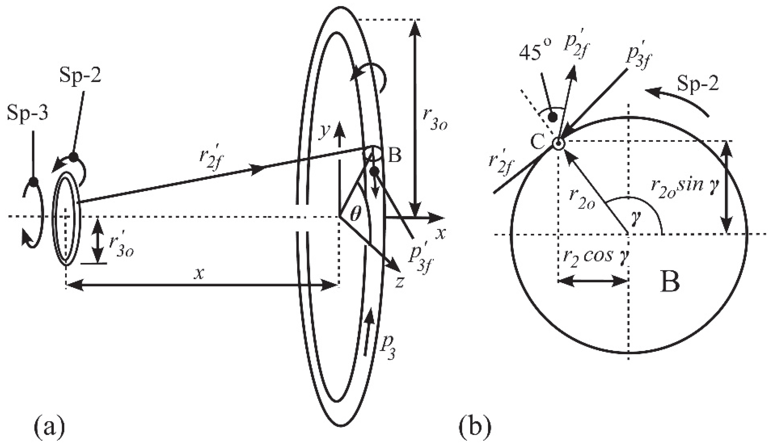
Following Ref. ([4], Equation (72) and Figure (13)), the in Equation (25) shows the number of electron Sp-2 circuits that are receptive to the change in proton field momentum. Here, is the total change in the mean magnetic momentum field around the Sp-2 circuits, is the Sp-2 proton field momentum in the locality of the electron, is the incremental unit tangent vector for the Sp-2 electron radius, and is the electron velocity vector along . Let be the distance between the proton and electron Sp-2 centers, taken perpendicular to their common toroidal axis, see Figure 4a, where . Then we have
having ignored powers of higher than first order ([4], Equation (70)).
The orientation of field vector introduces a geometric projection factor that reduces the effective field coupling, see Section 1.3.5. We represent both the proton and electron Sp-2 circuits rotating counter clockwise in Figure 7 as
Table 7.
Correction multipliers in Equation (35) for various groups of hyperfine states.
| State | |||||
|---|---|---|---|---|---|
| Multiplier |
Table 8.
Results for the magnitude of the hydrogen hyperfine shift from the mid-point hyperfine frequency (MHz) for various states using Equation (35). Relativistic reduced mass and increased proton speed adjustments are included. The experimental value is at the top ([20], Table 3), and the PTV value at the bottom. The error magnitude is given as hf-error.
Table 8.
Results for the magnitude of the hydrogen hyperfine shift from the mid-point hyperfine frequency (MHz) for various states using Equation (35). Relativistic reduced mass and increased proton speed adjustments are included. The experimental value is at the top ([20], Table 3), and the PTV value at the bottom. The error magnitude is given as hf-error.
| State | Experiment/ PTV model |
hf-error | State | Experiment/ PTV model |
hf-error |
|---|---|---|---|---|---|
|
|
|
||||
|
|
|
||||
|
|
|
||||
|
|
|
||||
|
|
|
||||
|
|
|
||||
|
|
|
||||
|
|
|
||||
|
|
|
||||
|
|
|
||||
|
|
|
||||
|
|
|
||||
|
|
|
||||
|
|
|
||||
|
|
|
A variation in controls the strength of the magnetic momentum field , while its direction vector, being independent of , ensures a parallel field in the locality of the electron.
As a result of the motion of the electron through the proton momentum-field, there is a change in the mean momentum around the Sp-2 electron ring during the time it takes to complete one electron Sp-2 circuit . From Equation (25) and the structure of the Sp-2 circuits—see Ref. ([4], Figure 13, Equation (72))—we have
The magnitude of the velocity vector that represents the displaced momentum out of the electron PTV along at the state boundary is given by ([4], Equation (50)), thus
Then from Equation (27) since
to first order in we arrive at the following
Equation (31) arises from same sense Sp-2 rotations and taken as positive which means that the electron is receding from the proton. If we reverse the sign of so that the proton and electron converge, the sign of Equation (31) becomes positive, then using Equation (29) the sign reverses again as in Equation (32). Here, we should keep in mind that at a state boundary, any additional momentum that is redistributed from the Sp-2 circuit into Sp-3 momentum joins the translational motion of the toroid on its helical trajectory at a rake of on the frustrum. Differentiation with respect to replaces with in the numerator of Equation (31) and use of Equation (29) gives
having used Equation (16) when introducing . A conversion from Joules to MHz has also been made using . Substituting primed (proton) variables for un-primed (electron) we also have ([4], Equations (63) and (70))
Noting that
Then using Equation (33), the Rydberg frequency from Table A1 (see associated footnote), and normalizing the length to with a division by gives
Here, is the normalised bound-state distance between the proton–electron Sp-2 centers ([4], Table 2). So since then . The negative sign of Equation (35) represents the case in which the proton and electron are converging ( decreasing) and their Sp-2 rotation senses are the same, see Table 6.20 The PTV model results for Equation (35) can be positive or negative and their magnitudes are shown against the experimental values in Table 8 for the half-splitting.21
The multipliers obtained by data-fitting are listed in Table 7 and produce good agreement with experiment. We note that gives accurate values for the states, meaning that these states need no adjustment, thus supporting the parallel field assumption.22 The values for in Equation (13) represent the proton moving towards the electron in the center of mass frame, see Table 1.
4. PTV and QED Errors
4.1. Lamb Shift
Table 4.
Comparison of the QED ([18], Table 4 end column) and PTV Lamb shift absolute errors for 16 states of hydrogen from Table 4 and Table 5. The error is given by Ref. ([18], p.600). All frequencies are in MHz.
| State | QED error | ) | ) |
|---|---|---|---|
For the QED calculations, the centroids of the hyperfine levels of atomic hydrogen are given by Ref. ([18], p.600, Table 4) relative to the state or ionization limit MHz. The error (MHz) between the experimentally determined values and the QED calculations which are listed as ‘QED error’ in Table 4 are also given in Ref. ([18], Table 4). The QED error for the state of MHz is discussed in Ref. ([18], p.600 second column). The PTV theory does not aim for the centroid but the mid-point value of the two hyperfine frequencies as calculated from values given by (Ref. [20], Table 3, Table 4 and Table 5). The empirically determined Equations (12), (13), and (22) are used to achieve this. The PTV Lamb shift for the ground state is times greater than the traditional Lamb shift frequency.23 So it is important to note that Table 4 is not a direct comparison, as the QED and PTV Lamb shifts are different intervals. The absolute errors between experiment and PTV theory for this shift, taken from Table 4 and Table 5. The PTV mean absolute error is MHz against the QED mean absolute of MHz.
4.2. Hyperfine Shift
While the QED calculation for the hyperfine splitting employs unequal displacements about the centroid—see Equation (4)—the PTV calculation uses an equal displacement above and below the mid-point of the two hyperfine levels, Equation (35). Table 10 shows the magnitude of the hyperfine shift in which all experimental values in the second column are taken from Ref. ([20], Table 3, Table 4 and Table 5) in MHz. The QED calculations for the states in the third column are given by Ref. ([22], Table 3), except the state which is provided by Ref. ([23], p.39). For the non- states, the QED values are taken from Ref. ([18], Table 1). All experimental values have been converted to a half-splitting for comparison with the PTV values. The PTV mean absolute error is MHz (median MHz) against the QED value of MHz. Taken over 30 states, the PTV value is MHz. All errors are given to the nearest kHz.
Table 10.
Comparison of the QED and PTV hydrogen hyperfine splitting absolute errors from Table 8. All values are in MHz.
Table 10.
Comparison of the QED and PTV hydrogen hyperfine splitting absolute errors from Table 8. All values are in MHz.
| State | Experiment | QED calc. | PTV calc. | QED error | PTV error |
|---|---|---|---|---|---|
5. Extension to Other Isotopes
5.1. Deuterium Validation
We now replace with in (Ref. [4], first of Equation (35)) where . This is the electron self-potential angular momentum. Also, we allow the nuclear Sp-3 angular momentum to become in Ref. ([4], Equation (74)) where . This affects the nuclear Sp-3 field. For deuterium, we replace the proton mass with , and similar to hydrogen and .24 As with hydrogen, a search is conducted for in Eqs (12) and (13) that yields the most consistent values using Equation (23). We then search through the in Equation (22) to minimize in Equation (24). The values of , , , and for deuterium are given in Table 11 and Table 12. Unlike hydrogen, does not minimize to zero which suggests that a more intricate mechanism for the nucleus is at work than that for Equation (22) with hydrogen. However, the minima produced for give a mean absolute error of MHz (see Table 13), and for a mean absolute error of MHz, with the same 18 states tested in each case.
Table 11.
The optimized radiation exit shift constants in Equation (22) for 18 states of deuterium , , and , for in Equations (13) and (22).
Table 11.
The optimized radiation exit shift constants in Equation (22) for 18 states of deuterium , , and , for in Equations (13) and (22).
| States | (MHz) | (MHz) | ||
|---|---|---|---|---|
Table 12.
The optimized radiation exit shift constants in Equation (22) for 18 states of deuterium , , and , for in Equations (13) and (22).
Table 12.
The optimized radiation exit shift constants in Equation (22) for 18 states of deuterium , , and , for in Equations (13) and (22).
| States | (MHz) | (MHz) | ||
|---|---|---|---|---|
Table 13.
Deuterium hyperfine mid-point results for the red shift (Table 6), with the states (), states (), and states (). The experimental mid-point hyperfine values ([18], Table 6) are the top values, and the optimized values given by Equations (12), (13), and (22) are the lower values.
| State |
(MHz) |
(MHz) | State |
(MHz) |
(MHz) |
|---|---|---|---|---|---|
|
|
|
||||
|
|
|
||||
|
|
|
||||
|
|
|
||||
|
|
|
||||
|
|
|
||||
|
|
|
||||
|
|
|
||||
|
|
|
From Table 6 and Table 7, the mean value of taken across the six sets of states. The experimental hyperfine mid-points in Table 8 are calculated from the centroids in Ref. ([20], Table 6) taking into account the ratio of the splitting about the centroid.
The hyperfine shifts are shown in Table 14. For deuterium, Equation (35) now needs an extra universal multiplier of which applies across all deuterium states, and for in Table 7. This suggests that the Sp-2 magnetic momentum field of the deuterium nucleus has a smaller effect than that of hydrogen which needs no universal multiplier. The mean value of the absolute errors hf-error in Table 14 is MHz.
5.2. Nuclear Mass Number Scaling
Data for only three states has been found for tritium ([18], Table 8) and an investigation shows that similar to deuterium, the gradient difference in Equation (23) does not minimize as effectively as for hydrogen but nevertheless exhibits non-zero minima for both and . The proton mass now becomes . Here, and , the same values as those for hydrogen and deuterium. This data is shown in Table 15.
Table 15.
The optimized radiation exit shift constants in Equation (22) for 3 states of tritium for both signs of in Equations (13) and (22).
Table 15.
The optimized radiation exit shift constants in Equation (22) for 3 states of tritium for both signs of in Equations (13) and (22).
| States | (MHz) | (MHz) | ||
|---|---|---|---|---|
The mean value of MHz. This brings us to a nuclear scaling law for hydrogen, deuterium, and tritium in which
where is the nuclear mass number.
5.3. Nuclear Charge Effects
We now investigate the value of for 3He+ which consists of two protons and one neutron (), but carries a nuclear charge of . This is the number we associate with the unloaded PTV self-potential angular momentum in Ref. ([4], first of Equation (35)) in which becomes . We also set which means that every in Equation (12) is replaced by . These values produce the smallest difference in gradients using Equation (23) when obtaining and both must appear in the optimization search Ref. ([4], Equation (85)), to find the bound-state distance in Ref. ([4], Equation (86)). Table 16 shows the results of the investigation for the states.
Table 16.
The optimized radiation exit shift constants in Equation (22) for 3 states of 3He+ for both signs of in Equations (13) and (22).
Table 16.
The optimized radiation exit shift constants in Equation (22) for 3 states of 3He+ for both signs of in Equations (13) and (22).
| States | (MHz) | (MHz) | ||
|---|---|---|---|---|
The mean value of MHz. A preliminary investigation for 7Li2+ () on the states using and has shown that for , , and we have . With we obtain . Their mean value is shown in Table 17.
5.4. Universal Nuclear Scaling Law
We now suggest a scaling law for nuclei relative to the mean-value hydrogen result as follows:
where is the nuclear charge which in the PTV model is the nuclear Sp-3 angular momentum . The appears in the internal-potential term in Ref. ([4], Equations (31) and (35)) so that the or is replaced with or , respectively. The accuracy of Equation (37) is summarized in Table 17.
Table 17.
Comparison of theory with PTV model for the universal scaling law applied to hydrogen, deuterium, tritium, 3He+, and 7Li2+. The PTV prediction for modelled on experiment is compared with the theoretical values from Equation (37).
Table 17.
Comparison of theory with PTV model for the universal scaling law applied to hydrogen, deuterium, tritium, 3He+, and 7Li2+. The PTV prediction for modelled on experiment is compared with the theoretical values from Equation (37).
| Element | PTV (MHz) | Equation (37) (MHz) | % error magnitude | |||
|---|---|---|---|---|---|---|
| H | ||||||
| D | ||||||
| T | ||||||
| 3He+ | ||||||
| 7Li2+ |
6. Conclusions
6.1. Physical Interpretation
The strength of the PTV model lies in its development of a visualizable mechanism for atomic spectra and the accuracy achieved suggests that geometrical approaches merit further attention. This architecture represents electrons and protons as helical string-like structures in optical OAM (Sp-2) with trajectories that are diverted into a toroidal structure (Sp-3). The Sp-2 and Sp-3 rotations are responsible for magnetic and electric effects, respectively. Within the model, interactions become exchanges of geometric momentum: the proton’s Sp-3 field occupies the electron PTV and displaces one half of its rotational energy into emissible translational energy to form a bound state. The hyperfine interaction is represented as a change in the proton Sp-2 field integrated around the electron Sp-2 circuit.
The observed field-free quantization of electron vortex beams [6,7,8], in which high-integer angular momenta can be generated without an external potential, suggest that non-vortex-beam electrons might also have this property. PTV theory introduces an effective internal potential that allows quantized states to occur without explicit reliance on the Coulomb potential on which the Sommerfeld–Dirac theories depend. In bound-state systems between PTVs of vastly different mass such as hydrogen (), the more massive PTV effectively defines the reference frame for the measurement of radiation emissions. While both Sp-3 fields displace the other’s Sp-3 momentum into translational motion, only the lighter PTV’s emission contributes to the observed spectral line. The more massive PTV continues its translational motion (induced by the lighter PTV’s Sp-3 field) while the electron’s motion is taken relative to the proton field in its Sp-3 rotation through the introduction of the reduced mass. Transitions arise as differences between Sp-3 rotational frequencies, and the occurrence of emission or absorption depends on the relative rotation senses of the incident radiation and the target Sp-3 level.
PTV applies the same three state-independent calculations to all 60 hydrogen states tested: 30 states with (red shifts) and (blue shifts). These calculations are the modified fine-structure Equation (12), magnetic potential adjustment Equation (22), and the hyperfine shift Equation (35). The parameters , , , and exhibit systematic behaviour: and are connected by a universal scaling law Equation (37) that applies across hydrogen, deuterium, tritium, 3He+, and 7Li2+; in Equation (22), across all states tested; and in Equation (35), for all hydrogen states is a prediction that supports the parallel-field approximation. A preliminary investigation shows that varying the eccentricity of the electron Sp-2 circuits while maintaining a constant perimeter can appropriately reduce the receptivity of these circuits to the varying proton Sp-2 field, and account for the various in Table 7. These patterns in the parameters address the objection of ‘curve fitting’ by providing evidence of an underlying geometrical structure to atomic processes.
Deuterium supports the model’s extension to composite nuclei: absolute hyperfine mid-point frequencies achieve 22 parts per billion accuracy (Table 13: MHz error at MHz for and ), while hyperfine shifts show at most % error. This demonstrates that energy-balance and Sp-2 principles can be suitably approximated by the hydrogen PTV model for systems with light nuclei.
The universal scaling of the -function parameter with the magnetic potential parameter A with nuclear mass number reflects an inherent reciprocity: a spatial differentiation of the Sp-2 momentum field followed by integration over the spatial trajectory from infinity to the bound-state displacement, yielding an endpoint-defined interaction energy. Within the Sp-2 framework, Sp-2 momentum fields are reciprocal, so this operation applies equally to electron and nuclear vortices. The apparent static character of the resulting interaction reflects the cancellation of the spatial differentiation by the spatial integration rather than the absence of underlying dynamics.
The PTV approach demonstrates that computational simplicity need not imply conceptual simplicity. While individual calculations remain calculator-executable (see Appendix B), their mutual consistency across fine structure, Lamb shift, and hyperfine splitting requires careful geometric coordination. This architectural coherence—where parameters determined for one phenomenon constrain predictions for others—provides internal validation absent in purely phenomenological models.
6.2. Future Developments
The construction of more complex nuclei than hydrogen from PTVs is a task for future research. For hydrogen, two oppositely rotating Sp-3 vortices of different scale can bind, and the electron forms its bound state at the point when the nuclear Sp-3 momentum field has displaced half of the electron Sp-3 momentum into translational motion. This energy-balance condition ([4], Equation (85)) ensures that exactly half of the original electron Sp-3 energy radiates away. The half that is left in the electron produces a Sp-3 momentum field that displaces the same momentum out of the proton into translational motion. So both PTVs lose the same momentum which is that of the smaller PTV. The question is whether or not this can be applied to the construction of light nuclei. What needs to be investigated is whether or not a neutron might be composed from two proton-scale PTVs with opposite Sp-3 that possess (clockwise) and (counter clockwise). At the binding distance , each radiates away one half of its Sp-3 energy leaving and . These two oppositely rotating Sp-3 angular momenta cancel out to zero charge, while the Sp-2 angular momenta reinforce. This assumes that the Sp-2 and Sp-3 angular momenta are equal. This would be exactly the same physical process as hydrogen formation but at nuclear scale. Whether PTV ultimately explains nuclear binding energies on this basis or reveals limitations in geometric approaches, the present work demonstrates that visualization and formalism can coexist productively as complementary approaches.
Data Availability Statement
The hyperfine calculation for Equation (31), a Liberty BASIC computer program, and the data output for that program can be obtained at the following link: https://barryispuzzled.com/hyperfine.
Conflicts of Interest
On behalf of all authors, the corresponding author states that there is no conflict of interest.
Appendix A. CODATA Constants
Table A1 shows the values of the constants used in the new PVT calculations. In the following notation, primed variables refer to the proton and unprimed variables to the electron.
Table A1.
2018 CODATA values for constants used [24].
Appendix B. Example Calculation for the state ()
This is the calculation represented in Figure 5. Here . In general, we choose the appropriate , obtain the radiation exit-shift constants from Table 2, the hyperfine-splitting multipliers from Table 7, and the bound state separation distances from Ref. ([4], Table 2). The equations are then exactly the same as the following.
This example demonstrates the calculation for states where , requiring no empirical correction to the hyperfine splitting ( in Table 4) which supports the parallel field approximation. All energies have been converted to frequencies (MHz) by multiplying by . The CODATA constants used are given in Table 9.
STEP 1: Unadjusted fine structure calculation
The equation for this is obtained from Ref. ([4], Equation (51)) converted to frequency (MHz) by multiplying by .
Noting that we have26
STEP 2: Relativistic reduced mass adjustment
This is a calculation for the reduced electron rest mass which will be adjusted in Step 3. From Ref. ([4], Equation (88)) the electron rest mass (consisting of Sp-2 rest mass and Sp-3 constituents) is
Then the reduced mass becomes
So using the result from Step 1, the frequency in Equation (39) after replacing in by Equation (41) becomes
STEP 3: Relative-to-proton speed adjustment
This is part of the Lamb shift calculation that targets the mid-point of the hyperfine pair. Here, we shall use and the -function in Equation (13). We note that . From Table 2, we have for the state, so
The value in Equation (43) now multiplies each occurrence of in Equation (39) so that the is modified to
The relativistic mass is now
Then the updated reduced mass from Equation (41) becomes
Equation (39) must now be modified keeping in mind that also contains so it needs modification, so that
STEP 4: Magnetic potential red shift
So, from Equations (47) and (48), the hyperfine mid-point is now
This result is shown in Table 4.
STEP 5: Hyperfine red shift
Using Equation (35), there is now a hyperfine red shift from the hyperfine mid-point calculated in Equation (49).27 We have , from Table 7, and from Ref. ([4], Table 2). Here, is the Rydberg frequency, see Table 18.
So
Then
STEP 6: The hyperfine level
Combining these calculations involving red shifts we have
Then our calculated value is
The accuracy is better than 4 parts in billion.
| 1 | These equations have been modified from Johnson and Soff [17] to exhibit the units kg and MHz. |
| 2 | This is the alternative helical string model suggested by Clarke ([4], footnote 8) which appears to have greater possibilities than a non-rotating string advancing along its axis. |
| 3 | The bound state distance from the nucleus also increases but the Sp-3 radius remains constant. |
| 4 | This is unlikely to be detected in changing magnetic fields which only affect the rest mass as pure Sp-2 rotation. |
| 5 | Note when , we must have and . Also, from Ref. ([4], Equation (23)) we have for the unloaded case using Equation (7). |
| 6 | |
| 7 | The mechanism involves equal partitioning between radial and azimuthal momentum at the point of emission to create the spiral angle that is preserved during propagation. In fact, Ref. ([4], Figure 11a) should show the vectors as being at to the Sp-2 tangent. |
| 8 | The attraction and repulsion mechanisms are explained in Ref. [4], Section 4.1. |
| 9 | Any occurrence of is replaced by . |
| 10 | See Section 3.3 for the conditions for optimizing . |
| 11 | This is a reasonable assumption concerning phase relationship. In Ref. ([4], Figure 13a), as the interlaced helical strings progress together from left to right, points at the same height in the diagram are reached at time intervals of . If one point generates a momentum field that strikes the proton, the proton will have moved on by the time the next point on the electron Sp-2 structure is ready to generate a field. |
| 12 | In Ref. ([4], Equation (79)) the given time period is the time required to traverse the whole structure and should have instead of since there are wavelengths to traverse by the interlacings. |
| 13 | The reasoning here is that if the proton Sp-2 frequency is reduced with , the momentum is removed from the Sp-3 rotation to compensate for the loss of action. The proton must move towards the electron to reduce the Sp-3 action to its next sTable value, see also Ref. [4], Section 2.6. |
| 14 | Normalisation here means a division by the invariant electron Sp-3 radius (same for all states). |
| 15 | The errors are greatest for the lowest state of the set so this is the focus when optimizing . |
| 16 | Of course, both the proton and electron Sp-2 rotation senses each have two possibilities. |
| 17 | Oppositely-directed momenta involving field and circuit at this strong point means a net reduction in the target Sp-2 circuit, while same-directed momenta leads to a gain around the circuit. |
| 18 | The ends of the frustrum are the proton and electron toroidal areas, see Figure 7a. |
| 19 | [As Ref. ([4], footnote 27) indicates, the electron Sp-2 motion is envisaged as an iterative incremental change along followed by an incremental restoration of . |
| 20 | Note that an increasing (positive) in Equation (31) corresponds to electron motion away from the proton. |
| 21 | The experimental hyperfine mid-point is calculated from half the difference between the upper and lower hyperfine values [20, Table 3]. |
| 22 | If the reduced mass and -function are introduced into Equation (35) there is 1.1 MHz error for when . |
| 23 | For example, for the state, the QED Lamb shift is MHz against the PTV shift of MHz ( ). |
| 24 | This is intentionally chosen to be integer. The atomic mass 2.01355 amu produces greater errors. |
| 25 | Calculated from . |
| 26 | Using the CODATA constants we find that against . So there is a difference in the second decimal place. The value of is used in the fine structure calculation but the components are used in the hyperfine splitting as the discrepancy there is negligible. |
| 27 | This is a half-splitting on one side of the hyperfine mid-point. The case gives the blue shift on the other side. |
References
- Simulik, V.; Krivsky, I. Lamb shift in classical electrodynamical model of atom. In Third International Congress on Geometry, Integrability and Quantization June 14–23, 2001, Vama Bulgaria; Mladenov, I. M., Naber, G. L., Eds.; Coral Press: Sofia, 2001; pp. 410–430. [Google Scholar]
- Simulik, V.; Krivsky, I. Y. Relationship between the Maxwell and Dirac equations: symmetries, quantization, models of atom. Reports on mathematical physics 2002, 50, 315–328. [Google Scholar] [CrossRef]
- Verrall, S. C.; Atkins, M.; Kaminsky, A.; Friederick, E.; Otto, A.; Verall, K. S.; Lynch, P. Ground state quantum vortex proton model. Foundations of Physics 2023, 53, 28. [Google Scholar] [CrossRef]
- Clarke, B. R. A photonic toroidal model of the hydrogen atom fine structure. Quantum Studies: Mathematics and Foundations 2025, 12, 19. [Google Scholar] [CrossRef]
- Wan, C.; Cao, Q.; Chen, J.; Chong, A.; Zhan, Q. Toroidal vortices of light. Nat. Photon 2022, 16, 519–522, Supplementary information Figure S5a. [Google Scholar] [CrossRef]
- McMorran, B. J.; Agrawal, A.; Anderson, I. M.; Herzing, A. A.; Lezec, H. J.; McClelland, J. J.; Unguris, J. Electron vortex beams with high quanta of orbital angular momentum. Science 2011, 331, 192–195. [Google Scholar] [CrossRef] [PubMed]
- Uchida, M.; Tonomura, A. Generation of electron beams carrying orbital angular momentum. Nature 2010, 464, 737–739. [Google Scholar] [CrossRef] [PubMed]
- Verbeeck, J.; Tian, H.; Schattschneider, P. Production and application of electron vortex beams. Nature 2010, 467, 301–304. [Google Scholar] [CrossRef]
- Darwin, C. G. The wave equations for the electron. Proceedings of the Royal Society of London 1928, A118, 654–680. [Google Scholar]
- Dirac, P. A. M. The quantum theory of the electron. Proceedings of the Royal Society of London A 1928, 117, 610–624. [Google Scholar] [CrossRef]
- Sommerfeld, A. Zur quantentheorie de spektrallinien. Annalen der Physik 1916, 51, 125–167. [Google Scholar]
- Sommerfeld, A. Atomic Structure and Spectral Lines, translated into English by Henry Brose (Methuen & Co., 1923), pp.473, 551–52, Appendix A.
- Leach, J.; Keen, S.; Padgett, M. J.; Saunter, C.; Love, G. D. Direct measurement of the skew angle of the Poynting vector in a helically phased beam. Optics Express 2006, 14, 11919–11924. [Google Scholar] [CrossRef]
- Lamb, W. E.; Retherford, R. C. Fine structure of the hydrogen atom. Physical Review 1947, 72, 241–243. [Google Scholar] [CrossRef]
- Bethe, H. A.; Brown, L. M.; Stehn, J. R. Numerical value of the Lamb shift. Physical Review 1950, 77, 370. [Google Scholar] [CrossRef]
- Eides, M. I.; Grotsh, H.; Shelyuto, V. A. Theory of light hydrogen atoms. Physics Reports 2001, 342, 63–261. [Google Scholar] [CrossRef]
- Johnson, and , W. R.; Soff, G. The Lamb shift in hydrogen-like atoms, 1 ≤ Z ≤ 110. Atomic Data and Nuclear Data 1985, 33, 405–446. [Google Scholar] [CrossRef]
- Kramida, A.E. A critical compilation of experimental data on spectral lines and energy levels of hydrogen, deuterium, and tritium. Atomic Data and Nuclear Tables 2010, 96, 6. [Google Scholar] [CrossRef]
- Bransden, B.H.; Joachain, C. J. Physics of Atoms and Molecules (Pearson, 2003), Equation (5.157).
- Horbatsch, M.; Hessels, E. A. Tabulation of the bound-state energies of atomic hydrogen. Physical Review A 2016, 93, 022513, Tables III, IV, V. [Google Scholar] [CrossRef]
- Clarke, B.R. Reinterpretation of the Grangier experiment using a multiple-triggering single-photon model. Modern Physics Letters B 2023, 37, 2350042. [Google Scholar] [CrossRef]
- Jentschura, U.; Yerokin, V. A. Physical Review A 2006, 73, 062503. [CrossRef]
- Karshenboim, S. G. Precision physics of simple atoms: QED tests, nuclear structure and fundamental constants. Physics Reports 2005, 422, 1–63. [Google Scholar] [CrossRef]
- Tiesinga, E.; Mohr, P. J.; Newell, D. B.; Taylor, B. N. CODATA recommended values of the fundamental physical constants: 2018, Reviews of Modern Physics 93 (April–June 2021), Tables XXX and XXXI.
Figure 1.
The magnitude of the ground state of hydrogen as calculated by QED [17]. The adjusted fine structure result with reduced mass is shown from Equations (1) and (2), the Lamb shift to the hyperfine centroid is obtained from Equation (3), and the hyperfine splitting is calculated from Equation (6) ([19], p.240).
Figure 1.
The magnitude of the ground state of hydrogen as calculated by QED [17]. The adjusted fine structure result with reduced mass is shown from Equations (1) and (2), the Lamb shift to the hyperfine centroid is obtained from Equation (3), and the hyperfine splitting is calculated from Equation (6) ([19], p.240).
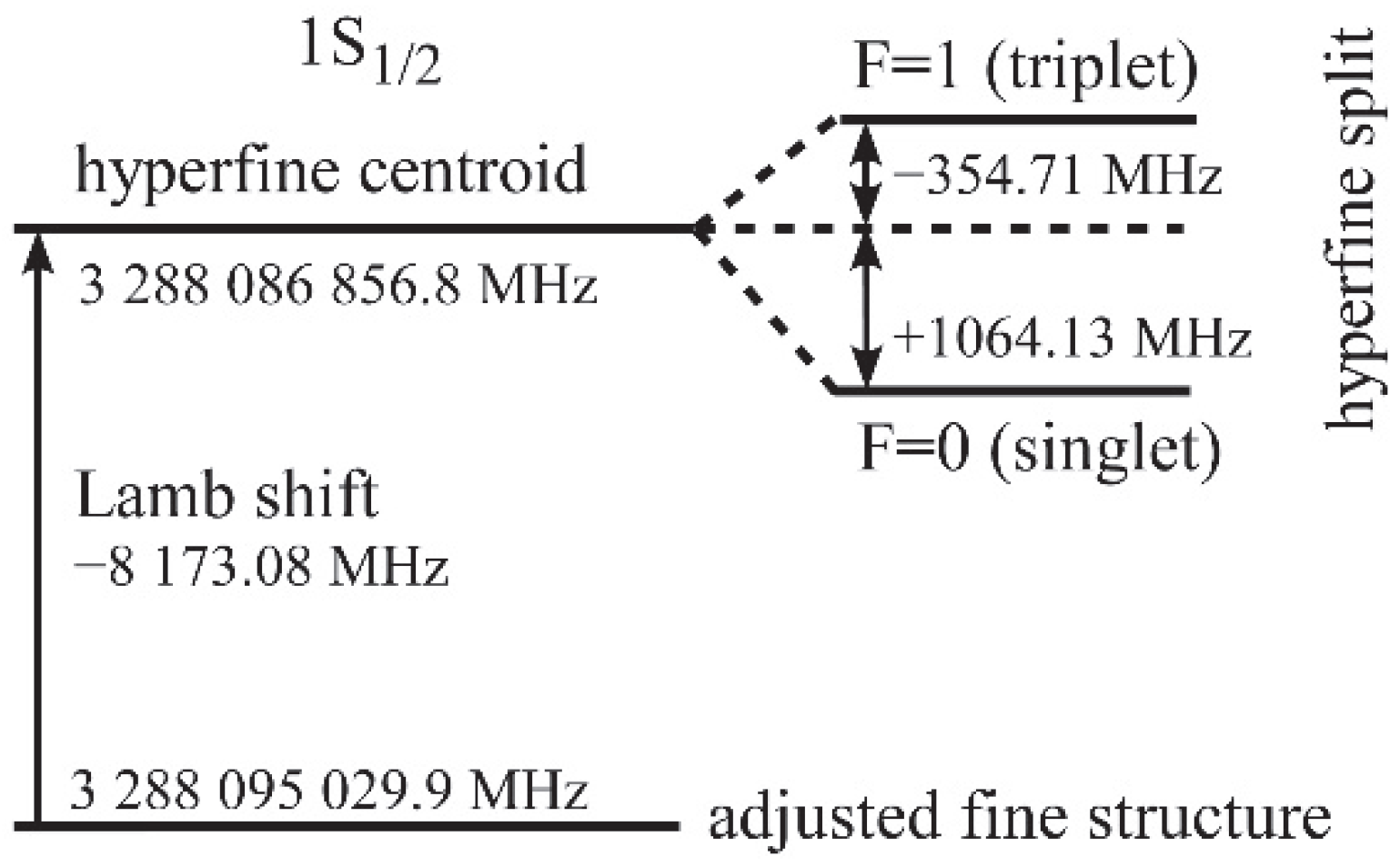
Figure 2.
a A string following a helical path at speed and rake has both azimuthal and linear speed c. b Net of the helical string in a with wavelength .
Figure 2.
a A string following a helical path at speed and rake has both azimuthal and linear speed c. b Net of the helical string in a with wavelength .
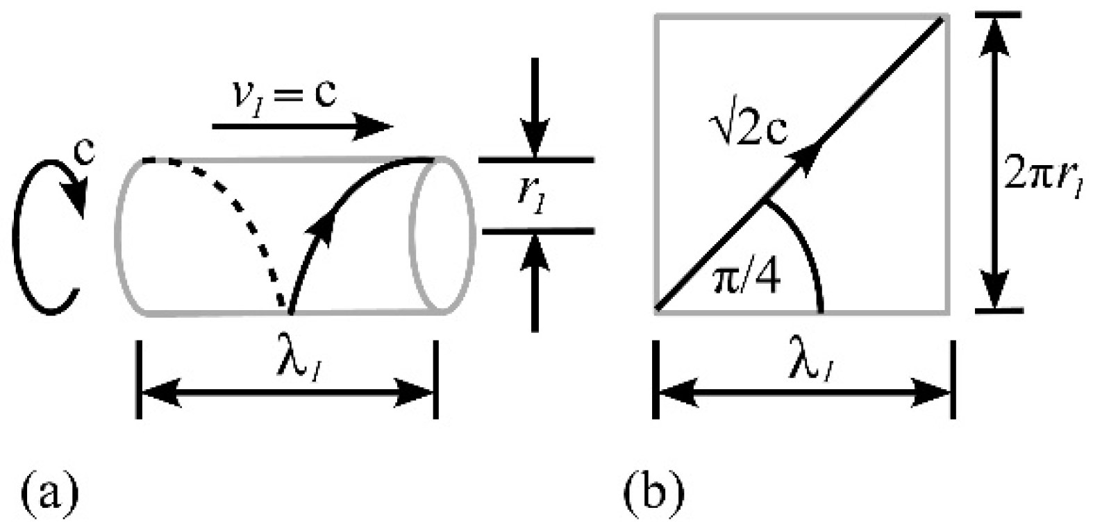
Table 14.
Results for the deuterium hyperfine shift from the mid-point hyperfine frequency (MHz) for various states using Equation (35). The experimental value is at the top ([18], Table 2), and the PTV value at the bottom. The error magnitude is given as hf-error.
| State | Experiment/ PTV model |
hf-error | State | Experiment/ PTV model |
hf-error |
|---|---|---|---|---|---|
|
|
|
||||
|
|
|
||||
|
|
|
||||
|
|
|
||||
|
|
|
||||
|
|
|
||||
|
|
|
||||
|
|
|
||||
|
|
|
Disclaimer/Publisher’s Note: The statements, opinions and data contained in all publications are solely those of the individual author(s) and contributor(s) and not of MDPI and/or the editor(s). MDPI and/or the editor(s) disclaim responsibility for any injury to people or property resulting from any ideas, methods, instructions or products referred to in the content. |
© 2026 by the authors. Licensee MDPI, Basel, Switzerland. This article is an open access article distributed under the terms and conditions of the Creative Commons Attribution (CC BY) license (http://creativecommons.org/licenses/by/4.0/).
Copyright: This open access article is published under a Creative Commons CC BY 4.0 license, which permit the free download, distribution, and reuse, provided that the author and preprint are cited in any reuse.