

Submitted:
21 March 2026
Posted:
23 March 2026
You are already at the latest version
Abstract
We will present numerical methods for solving initial value problems using an indefinite integral approach. This new method allows controlling the order of approximation as well as the number of discretization steps. The methods allow an a priori estimation of the approximation error, so that an optimized solution may be accessible. The approach is based on representing indefinite integrals using discretization over conformal mappings or orthogonal polynomial roots. Using these discretizations, matrices for implicit Runge-Kutta procedures are created using collocation methods.
Keywords:
initial value problem
; indefinite integral
; implicit Runge-Kutta
; Sinc method
; orthogonal polynomial
; Lagrange polynomial
; generalized Lagrange interpolation
; stability
; order star
1. Introduction
Differential equations are well-known among scientists as useful tools for scientific modeling. In this introductory discussion, we do not want to rehash what has already been said in numerous books and articles; see e.g. [1] and references therein, but rather to present widely recognized ideas in the terminology that will be used throughout the rest of this article.
Let us consider a system of ordinary differential equation (ODE) which can be stated in a compact form in the following form:
i.e. where n is the dimension of the solution space. The dash in (1) represents differentiation with respect to the independent variable, say t, which commonly represents time in dynamical systems. The dependent variables y are known as state variables, whereas is a collection of parameters represented as a vector. When addressing the components of a vector differential equation, we use the term “system of differential equations” to refer to equation (1).
Using a differential equation to represent the development of a state vector y in a physical process poses the challenge of predicting future values of y based on the starting or initial value of y. The mathematical model is represented by a set of equations. Using a system of differential equations to represent the evolution of a state vector in a physical process presents the difficulty of forecasting future values based on the initial value . This system of equations in connection with (1) serves as the representation for the mathematical model in the initial state.
Every system of ordinary differential equations (1) is equivalent to a single differential equation including a higher derivative. The inverse of this assertion is true for higher-order differential equations, which can be solved to the highest order. As a result, we shall confine our discussion to systems of ordinary differential equations in the form (1).
For the system of first-order ordinary differential equations (1), we will provide numerical solution approaches based on implicit Runge-Kutta (RK) procedures. These approaches are primarily dependent on the presence of discrete representations of indefinite integrals . In other words, we shall demonstrate a significant numerical application of indefinite integrals to implicit Runge-Kutta techniques. We shall demonstrate that the discrete formulation of indefinite integrals leads directly to the numerical integration of initial value problems.
In this regard, there is nothing new; because indefinite integrals may be utilized to solve initial value problems via direct integration. What is new is that the Runge-Kutta techniques can now include the discretization of indefinite integrals in different forms. This generalizes to a large variety of indefinite integral representations using Sinc techniques or orthogonal polynomial (OP) roots [2,3]. We’ll utilize both Sinc and root based approaches.
The generalization stems from the finding that indefinite integration is the ancestor of the Runge-Kutta technique. We employ Sinc, Sinc-Exp, Lagrange and generalized Lagrangian interpolation for indefinite integration, which in this particular instance uses either Sinc functions or orthogonal polynomials as basis, respectively [3,4].
Runge and Kutta [5,6] developed a numerical solution process that allows for both explicit and implicit representations of calculation formulae. The explicit Runge-Kutta technique is simple to use, but the implicit Runge-Kutta approach needs a simultaneous system of equations to be solved at each step. Except for f being linear in y, they are nonlinear equations. For the first approach to discuss the relations, we use a scalar ODE to clearly demonstrate the links. Here, we will look at scalar initial value problems of the type
where . Furthermore, we assume that they are non-stiff or stiff ODEs. In the context of stiff ODEs, Hairer and Wanner‘s work [8] has to be noted. Nonetheless, it will become clear that our method, which is based on the definition of indefinite integrals, can handle both stiff and non-stiff ODEs. The method is not new in and of itself; it dates back to the 1960s of the previous century. The Runge-Kutta technique can be reduced to indefinite integrals in a collocation process, as Guillou and Soulé discussed in a 1969 paper [9]. Wright’s publication [10] contained additional verification of this. This approach provides an estimate for both explicit and implicit Runge-Kutta methods presentations.
Some kinds of ordinary differential equations can be easily solved numerically using the Runge-Kutta technique. However, deriving high-order Runge-Kutta techniques can be a challenging undertaking. This is due to a variety of factors. Identifying the so-called order criteria is the first problem [1]. To make the error in the process of order for some digits, these nonlinear equations need to be met. Solving these equations is the second obstacle. In addition to being nonlinear, several heuristics and simplifying assumptions are typically used, and there is typically no unique solution. The problem of combinatorial explosion is another. To give an idea on the related problems, a twelfth-order approach has 7813 order criteria exploding the efficiency [1]. To avoid all these mentioned obstacles we take here the route via indefinite integration.
The article is structured as follows: Section 2 discusses the key features of indefinite integrals and Runge-Kutta techniques. Section 3 describes three methods for approximating indefinite integrals. Section 4 applies the methods described in Section 3 to implicit Runge-Kutta procedures. Section 5 discussed the stability problem of the implicit Runge-Kutta method. Section 6 uses examples to show the solution of stiff and non-stiff initial value problems. Section 7 summarizes the findings and addresses unresolved questions.
2. Methods
This section covers the principles of the implicit Runge-Kutta technique. The principles of indefinite integrals provide an important foundation for explaining the numerical technique, which is based on the collocation of a Volterra integral equation.
2.1. Indefinite Integrals
This section covers the numerical computation of indefinite integrals for a function . We use the notation for the generic operators defined by the two following relations:
and
The two operators are linear i.e.
Inspection provides the proof. Another characteristic of is that the two operators are bounded [4]. In the following, we will investigate how the indefinite integral operators may be represented by Sinc, Sinc-Gaussian, or Poly-Sinc methods, respectively. However, let us first discus the connection between indefinite integrals and Runge-Kutta methods.
2.2. Runge-Kutta Method
We start with the initial value problem (2) and represent it as an integral equation
To obtain a numerically approximate solution to this problem, we will choose a sequence of values and we will define, step by step, approximations (with vector coefficients) ,..., ,... which will respectively approximate on the successive intervals , …, , …. Here the satisfies the following conditions:
- 1.
- , ,
- 2.
- with and .
Using a specific basis the derivative of y can be represented as an approximation in an Hilbert space as
using an s-order approximation. Contrary to the standard notation, we call the approximation an s-order approximation to indicate the order of the approximating matrix which becomes clear in the following. This approximation results to the representation
and subsequently after discretization of t we get
Here denotes an matrix of order s. This leads us to the following method: determining the using the system of implicit equations
and the discrete approximation results to
where , , and with .
The integration matrix and the Runge-Kutta weights can be calculated by using integration as follows if the n discretization points are known, i.e., either the Sinc points or the roots of classical orthogonal polynomials:
and
with
where are either Sinc, Sinc-Exp functions, elementary Lagrange or elementary generalized Lagrange interpolation polynomials. Knowing this relations and the connection between discretization and the used base functions we will denote them as Sinc-RK, Sinc-Exp-RK, L-RK, and gL-RK methods, respectively. Integration in (13) and (14) is effectively based on Sinc quadrature [3,34]. Knowing the discretization vector , the integration matrix , and the Runge-Kutta weights enables the use of the Butcher tableaux [1], which summarizes the determining elements of a Runge-Kutta technique:
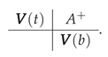
The tableaux allow us to classify the Runge-Kutta technique as explicit or implicit. If matrix is completely filled with nonzero elements, it is an implicit method. If matrix can be reduced to a triangular matrix, an explicit method is provided. In the above mentioned cases, we will always have to deal with implicit methods in our different approaches since matrix is completely filled. Because matrix is a matrix, which precisely defines the Runge-Kutta method, we can establish the method’s order using the dimension s. Contrary to commonly used nomenclature, we refer to s as the order of rather than the s-stage technique [1,8,11]. If we create with s discrete points , we have an s-order Runge-Kutta method. So we’ll utilize an implicit Runge-Kutta method of order s, which is derived from either a Sinc, Sinc-Exp, Lagrange, or a generalized Lagrange collocation.
3. Variants of Methods
In this section, we will look at the RK techniques’ discrete representations. The representation here refers to the discretization points and the precise basis elements used. We start with the Sinc approach, which takes translated Sinc functions as a base and discretizes over Sinc points. In the second technique, we utilize orthogonal polynomials as basis functions, with their roots used for discretization. In the final technique, we employ generalized Lagrange polynomials as a foundation, which are based on orthogonal polynomials, and discretize using Sinc points or orthogonal polynomial roots.
3.1. Sinc Methods
Let us start by providing two definitions that will be incredibly useful throughout the remainder of this article.
Definition 1
(Basic Definitions.). Let be a simply-connected domain having boundary . Let a and b denote two distinct points of , and let ϕ denote a conformal map of onto , where , such that , and . Let denote the inverse map, and let Γ be defined by
Given ϕ, ψ and a positive number h, let us set
Let us also define ρ by
Let , and let denote the family of all functions F that are analytic in , such that
Corresponding to numbers α and β, let denote the family of all functions for which there exists a constant C such that
for all z in . Finally, let us define by .
It is convenient to define yet another important family of functions, with , , and . The family consists of all those functions such that where
Just as for and , we define by .
Sinc methods rely on the and classes, which are easily recognized in applications. They also assure the quick convergence of the Sinc approximations presented in the next theorems, as well as the approximations utilized in subsequent sections and parts of this work (see also [2,3].
The second concept we’ll often employ is a set of basis functions for approximations. The next step in Sinc approximations is to define a Sinc basis, }, that uniformly approximates the functions F on the interval . For this reason, we provide the following definition.
Definition 2
(Sinc Basis.). Let the conformal maps ϕ be given. The density ρ is defined as in (19) for single exponential maps. Let the Sinc function be and the Sinc-Gaussian or Sinc-Exp be given as orthogonal basis functions, then by using
we are able to define the set of basis functions as follows
where is the inverse conformal map using the interval limits as additional parameters.
The functions defined in (25) meet the relation if , and if otherwise. This is nothing more than the interpolation condition. Note the piecewise definition changes only at the endpoints by interpolation to guaranty a nearly homogenous local error.
This notation allows us to define a row vector of basis functions
with defined as in (25). For a given vector we now introduce the dot product as an approximation of the function by
which is simply a Sinc or SG interpolation of a known function, in a single exponential representation.
Based on this notation, we will introduce in the next few subsections the different integrals we need [3].
3.1.1. Sinc and Sinc-Exp Approximation of Functions
In our approximations we will use two types of basis function a Sinc based and a Sinc-Gaussian based approximation. In general a basis function is used to represent the approximation of the function f as follows
where the basis functions are classified using the c parameter as
with represents the Sinc function and is the Sinc-Gaussian (S/G). The first type of approximation results to the representation
using the basis set of orthogonal functions
where is a conformal map. As discussed by Schmeisser and Stenger [12] a Sinc approximation of a function f can be given in connection with a Gaussian multiplier in the following representation
with a constant and denoting a conformal map. This type of approximation allows to represent a function on an arc with an exponential decaying accuracy [12]. As demonstrated in [12] the approximation works effective for analytic functions. The definition of the Sinc-Gaussian basis follows next
allowing us to write the approximation in a compact form as
Here, are the discrete points based on Sinc points . Note that the formulae also apply when single exponential conformal maps (SE) are replaced with double exponential maps (DE).
The following theorem states that both Sinc and Sinc-Gaussian approximations provide a bounded error.
Theorem 1
The proof of this theorem for the pure Sinc case is presented in [2], whereas [12] examines the case. The choice is near to optimal for an approximation in the space , in the sense that the error bound in Theorem 1 cannot be significantly improved regardless of the basis [13]. It is also optimum in the sense that the Lebesgue measure achieves an optimal value lower than the Chebyshev approximations [14].
3.1.2. Sinc Indefinite Integral
This subsection describes how indefinite integrals can be numerically defined [13] and how these definitions are related to the definition of definite integrals. For collocating an indefinite integral and for obtaining explicit approximations of the functions and defined by
and
We use the following basic relations [13]. Let denote the set of all integers, and let denote the complex plane. Let be given by and be defined by using
with the sine integral. This put us into position to write
If now denotes a one–to–one transformation of the interval onto the real line , let h denote a fixed positive number, and let the Sinc points be defined on by , , where denotes the inverse function of the conformal map . Let M and N be positive integers, set , and for a given function f defined on , define a diagonal matrix by . Let be a square Töplitz matrix of order m having , as its entry, so that
Define square matrices and by
where the superscript “T” denotes the transpose. The collocated representation of the indefinite integrals (36) and (37) are thus given by
and
These are collocated representations of the indefinite integrals defined in (36) and (37), respectively [3].
The following theorem then enables us to collocate (linear or non-linear, non-stiff or stiff) initial value problems over an interval or an arc.
Theorem 2
(Indefinite Integral Approximation [3]. ). Let for and , take M=[β N/α], where [x] denotes the greatest integer in x, and then set . If , and if then there exists a positive constant and independent of N,such that
and
and are constants independent of N.
3.1.3. Sinc-Exp Indefinite Integration
In this section we pose the question how to approximate indefinite integrals on a sub-domain of . The approximation will use our basis system introduced in Section 3.1.1. We will introduce in this section the second version of the basis systems; i.e. a Sinc-Gaussian basis. The Sinc Gaussian basis includes the Sinc basis by setting , it turns out that for both basis systems, we are able to get an approximation converging exponentially. Specifically we are interested in indefinite integrals of the two types
and
If the function f is approximated by one of the approximations given in Section 3.1.1, we write for ,
Scaling the variable and collocating the expression with respect to x, we end up with the representation
The collocation of the variable x delivers an integral which will be our target in the next steps.
Note with the integral simplifies to the expression . The discrete approximation of the integral thus becomes
with , and , and delivers the approximation of via
For the discrete approximation, we need to know the value of to be able to find the approximation of the indefinite representation
The matrix can be written as
reducing the problem to the structure of a Töplitz matrix if the indefinite integral has some finite values. To get the values of the integrals we divide the integration domain into two parts
The two integrals deliver in straight forward integration the following
and
with , and , thus . A similar procedure can be applied to the integral . The difference is a transposition of the matrix in the representation of approximation. The following Theorem summarizes the results.
Theorem 3
(Indefinite Integral Approximation.). If ϕ denotes a one–to–one transformation of the interval onto the real line , let h denote a fixed positive number, and let the Sinc points be defined on by , , where denotes the inverse function of the conformal map ϕ. Let M and N be positive integers, set , and for a given function f defined on , define the vector , and a diagonal matrix by . Let the vector of basis functions, and let be a square Töplitz matrix of order m having , as its entry, ,
Define square matrices and by
where the superscript “T” denotes the transpose. Then the indefinite integrals (47) and (48) are approximated by
where and are constants independent of N.
Note the matrices and have eigenvalues with which guaranties the convergence of the solution. A proof for the pure Sinc case for the matrix was recently given by Han and Xu [15].
If we use the properties of the matrices and defined above we know that
where is a matrix filled with 1’s and is antisymmetric. The elements of the diagonal matrix are all positive according to their definition. If we assume that is diagonalizable then for each eigenvalue there exists a complex valued eigenvector . Since the eigenvalues of are the same as we can write for for example
which is equivalent to
or
which is
in other terms
The real part of this expression delivers
the second term vanishes because the matrix is antisymmetric and thus since and we have
If we assume that the norm is defined on the vector space, we can use the Rayleigh quotient of a matrix H given by to bound the eigenvalues. According to [16,17] there exist a minimal and maximal eigenvalue defined by
and
Based on Grenander and Szegö theory [18], we may conclude that the eigenvalues of are strictly positive for finite matrix sizes.
3.2. Methods Using Orthogonal Polynomials
In this part, we will largely focus on approximation via interpolation at the roots of orthogonal polynomials . These polynomials include Legendre polynomials, Chebyshev polynomials, Gegenbauer polynomials, and Jacobi polynomials, which are initially defined on . We focus upon studying on the classical set of orthogonal polynomials. For information on other classes and their computations, refer to Gautschi [19]. The following presentation includes polynomials such as Laguerre- and Hermite polynomials defined on and .
For example we may categorize the orthogonal polynomials as:
- 1.
- For Legendre polynomials, are the n zeros of the Legendre polynomial , which are orthogonal on the interval with regard to the weight function w, which is identically 1 on .
- 2.
- For the case of Hermite polynomial interpolation, using the Hermite polynomials that are orthogonal over with respect to the weight function w , with , and with for ; and
- 3.
- Other polynomials that are orthogonal with respect to a weight function, such as Jacobi polynomials, Gegenbauer polynomials, etc.
We should remark that the approach presented here, indefinite integrals via root-based Lagrangian interpolation, is novel.
Let be a set of polynomials with degrees less than or equal to n, and be a smooth entire or analytic function defined on the interval . For the function , the interpolation polynomial fits the following requirements.
for n different root positions in . The discrete points , are taken as roots of orthogonal polynomials, as indicated before. The resulting polynomial of order meets the interpolation condition: for . The scenario is analogous to Lagrange polynomials.
A Lagrange polynomial approximation of order is:
where
are the discrete values based Lagrange polynomials employing with
The Lagrange polynomials satisfy the elementary interpolation requirement, as shown by
We can now estimate the global approximation error for an entire function f. The infimum of the absolute difference between f and the approximating order polynomial is roughly given as
If f is entire, then ; e.g. if then which delivers
The maximum occurs when we differentiate with respect to r and put the result equal to zero.
Solving the equation with respect to n yields a relationship between r and n which is . The solution for r then delivers Finally, this demonstrates that there is an error that decays as . This relationship confirms that the error relation becomes
The error thus comprises two important aspects. with , which is increasing; , which is decreasing. The maximum of the expression is assumed when . Because decays faster than the exponential function, the overall error as a function of n decays faster than the exponential function .
On the other hand, it is well known that if a function f is analytic in a simply connected domain D in the complex plane and if a closed interval is in the interior of D, then we can approximate f on via a polynomial of degree n for which the error approaches zero at a rate of , where is a positive constant. If the function f on D is entire, we are able to predict an error rate of as discussed above. If none of the two are correct, the usual error rate for polynomial approximation is . These three error rates will serve in the following as basis for the indefinite integral approximation based on Lagrange polynomials.
Based on those results and the Lagrange approximation provided above, let us look at the following two indefinite integrals.
and
It will be approximated with the aforementioned relationships. As a result, we offer the following Definition.
Definition 3
( Root Based Indefinite Integrals.). Consider generalized Lagrange interpolation at distinct points on , with , which takes the form
using the Lagrange interpolation for orthogonal polynomials
Referring to integral (84) and (85), we are able to define the entries of the matrices by the matrix elements as
and
where w is the weight function related to which is the set of classical orthogonal polynomials (see Olver et al., pp. 438 [20]), that is positive a.e. on , and is such that the moments exists for every non-negative integer j. The function w, where a.e. on defines a sequence of orthogonal polynomials , for which all n zeros of are located on .
Now, setting
and
where are the basic Lagrange polynomials (77). We are defining by
we obtain a practicable approximation of an indefinite integral using standard Lagrange interpolation. Assuming our function f is either entire, analytic, or none of the two, we obtain the error decay of the approximation provided by either the relation (83), exponential, or , respectively.
3.3. Generalized Lagrange Methods
Aitken and Neville suggested a generalization of the Lagrange interpolation in 1932 [21,22], followed by Mühlbach [23]. The numerical computations were performed using an iterative technique. Occorsio and Russo [24] recently employed an iterative technique, while Moalemi presented a generalization in analytic form in her PhD thesis [25]. Cheney and Light discuss a more general form of Lagrange interpolation [26]. With prescribed nodes ,…, in X, where X is an arbitrary set, they define
and is a function such that if and only if . Therefore,
and the interpolating polynomial is defined by using and interpolates the function f.
We will briefly discuss the method used in [25] and then apply it to the set of classical orthogonal polynomials in this section.
Consider be a set of continuous functions defined on so that for and represent n unique discretization locations in . The generalized Lagrange function for is defined as follows:
using the index set given by:
The interpolation condition is directly verified in (95) by
This implies that the collection of basic functions represents a collection of linearly independent functions on . In other terms:
creates an interpolation space that enables for representation:
satisfying
ensuring a unique interpolation function, therefore establishing a Chebyshev system [27].
To construct the basis , it is first necessary to have a sequence of discrete numbers , which can be any numbers satisfying for . This set is used in conjunction with another set of functions to form the generalized Lagrange basis using (95). It is important that the interplay between the two sets X and is independent of the discrete function values .
For the specific interpolation we will develop, we are employing the classical normal orthogonal polynomials. For , we put . Where . For the discretization points, we utilize the roots of the polynomial . Note that the distribution of roots on is not equidistant.
Thus equation (95) takes the form:
with roots satisfying and . This allows to write the interpolation of as
This put us into position to introduce vectors for numeric representation as follows
and
delivering a direct representation of the interpolation polynomial as an analytic representation
This formula is straight forward and can be implemented in a direct way.
The same steps can be used to approximate by:
with
In addition we have the approximation of a quadrature rule as
delivering
Note that the selection of the orthogonal polynomial type determines the coefficient matrix .
Now we are in position to set
and
so that an approximation of can be defined as by
Thus, we obtain a practicable approximation of an indefinite integral using generalized Lagrange interpolation. In addition we find
We may now use the introduced matrices and vectors to formulate the implicit Runge Kutta technique, which provides an approximation to an initial value problem.
4. Runge Kutta Method
So far, we’ve demonstrated that indefinite integration techniques are defined by the matrices . Because the matrices’ representations are based on distinct underlying basis systems and discretization methods, it is only appropriate to refer to various Runge-Kutta procedures.
Given the discretization , the matrix defined as in (60), (65), (88), or (107), and weights based on (14) the one-step Runge-Kutta iteration (12) can be transformed to an iterative multistep formula using the following iterations:
where is the individual step length. The notation denotes the kth iteration step and .
The resultant discrete solution points , with may now be used in an interpolation to get a representation of order N as an analytical function of the solution to the initial value problem:
where is the set of basis functions which are either Sinc, Sinc-Exp functions, Lagrange, or generalized Lagrange polynomials, respectively.
5. Stability
In previous sections, we looked at the convergence and error behavior of the Sinc-, L-, and gL-RK algorithms. The matrix of indefinite integration serves as the basis for all three approaches. In this section, we’d like to discuss another element of these RK methods: their stability. The geometric features of the RK approaches can be exploited to do this. We shall employ the stability function , often known as the Padé approximation.
These findings are based on a stability study by Dahlquist [28]. A linear stability analysis assumes that any initial value problem,
may be linearized to
which represents the behavior of stiff systems in the vicinity of a stationary point. The eigenvalues of the Jacobian matrix determined at the stability point are denoted as . If the real parts of the ’s are negative we speak of stable behavior; i.e. the equation is stable in the sense of Lyapunov when . It is widely known that the solutions to the differential system in (119) decline exponentially as . Applying a RK one-step approach which in general is a relation of the form to this equation results to
where . The RK method’s stability function is denoted as . This means necessarily that if , we have stability. The stability domain, defined as , is the set of points in the complex plane where the calculated solution stays bounded after several steps of computing. To meet the stability condition, all eigenvalues , multiplied by step size h, must be in . If , the solution of (120) will be in a single h-step operation. In the same time span, the approximate solution computed with a RK method will be multiplied by a z-specific function . Values of z in the left half-plane are of particular importance since the precise solution is bounded in this instance, and proper problem modelling requires the computed solution to behave similarly.
As discussed above the following tableau defines an s-order RK method
In contrast to the literature, we shall refer to it as an s-order RK method rather than an s-stage RK method because here is always of order . The vector , consisting of the s order values, satisfies
where is the initial approximation. It follows that
Substitute this into the solution approximation determined at the end of the steps, we get
where
Continuing the iteration, we discover
where
here ⊗ represents the Kronecker product. As already mentioned the function is called the stability function. Thus the condition that as is equivalent to . This motivates the definition of a region of absolute stability which is a set [28]. A Runge-Kutta method is called A-stable if the region of absolute stability contains the set . As Dahlquist stated in his work, “In most applications A-stability is not a necessary property.” [28]. This indicates that for application purposes, the word global stability has precedence [11]. The stability function of a Runge-Kutta method with matrix and is thus defined by
where denotes the vector with all ones. According to Ehle [29], the stability functions of high-order implicit Runge-Kutta methods are Padé approximations to the exponential function . Ehle’s Conjecture states that only the diagonal Padé and the first two subdiagonals are A-stable. is a rational function of the form
with a kth degree polynomial and is a polynomial of degree l. Here denotes the Padé approximation of order .
In addition, we wish to show how with creates geometric shapes that correspond to ordered star structures. To do this, we first apply the Ehle representation of the Pade approximation to polynomials that are the same as the Kummer confluent hypergeometric function in a finite representation [20]
and
The answer to Dahlquist’s initial value problem (120) is , which is represented as a rational polynomial using Ehle’s polynomial representation. Considering Ehle’s solution, we can see that the Padé representation is dependent on the order of the polynomials k and l. This results in k zeros and l poles for the solution, depending on the order of approximation. The zeros of the divisor polynomial determine the poles. The link between the Padé approximation and the solution method’s stability function allows us to investigate the interaction between them. Because the Padé approximation gives an approximate solution for the exponential function, it is beneficial to describe it as an approximation of order . This can be expressed as the following relationship:
or in a more accurate form
If then is unique.
The key aspect here is that a Padé approximation or stability function is determined only by the basis and the type of discretization used. Thus, an RK method’s stability is exclusively defined by the matrix structure and the weights given by (13) and (14), respectively.
Hairer et al. and Iserles et al. conducted investigations on this type of problem using order stars in the 1990s and compiled the findings in their works, which included multiple references on this subject [7,8,51].
Example 1
(Geometry of Padé Approximation.). We use the Dahlquist solution as an example to show how this geometric analysis approach works. We use a Padé approximant to compare with the solution . The right-hand half determines the absolute value of the ratio , while the contour for is also calculated. We color this region blue, beginning with red for value 1 and ending with 0. This coloration indicates the absolute magnitude of the ratio. The zeros of the Padé approximant are shown as dots in red (•), encircled by a color for values less than one. The stars in green (★) on ’s right half-plane depict the Padé approximant’s poles. The hue around these poles is white, suggesting that the absolute ratio is larger than one in this area. The general distribution of zeros and poles is star-shaped see Figure 1. This is also the meaning behind the name, which means “ordered stars.”
Order stars is a simplified depiction of the context for the geometric study of the distribution of zeros and poles when approximating an entire function, such as the exponential function. The idealization is that we can establish the structure of the Padé approximants using the order of the Kummer functions, yielding an analytical representation of the solution function. The second point of simplification is that the solution function, , is known. However, this is rarely the case when using an RK technique. Nonetheless, the situation is not hopeless, since we know that a Padé approximant exists for generic functions; for a comprehensive discussion see [52,53,54]. ▴
Example 2
(Order Stars for gL-RK Methods.). As a fundamental illustration of the gL-RK method’s stability, we take one-parameter Gegenbauer polynomials as a basis, as well as independent discretization with Legendre and Chebyshev polynomials.
First, using the Gegenbauer polynomials as basis, we have to deal with m as a influencing parameter. On the other hand, because we know that the discretization of the matrix affects the poles in the complex plane; compare with the Ehle representation (133), and that the basis affects the placement of the zeros due to relation (128), we can influence the stability by varying both driving factors. In Figure 2, we show the computations with Gegenbauer polynomials as a basis, as well as the Legendre and Chebyshev polynomials used to discretize the matrix . Even when the parameter value , no differences are seen as compared to the discussion in [55]. This leads us to the conclusion that the discretization of matrix is primarily responsible for stability. We reiterate that the step size is implicitly defined by the approximation order and polynomial type. The approach does not use a set step size, but rather a variable one defined by the root distribution of the polynomial type.
6. Applications
This section provides examples of the use of implicit Runge-Kutta procedures. The numerical processes have been implemented in Mathematica and are available in our book, “Applied Sinc Approximations: Polynomial and Sinc Methods for Solving Calculus Problems in Mathematica” [34]. We will not detail the implementation here, but will instead provide findings for particular scenarios. The interested reader can discover the essential functions and methods in [34].
Example 3
(Gaussian Problem solved using Sinc-RK.). We define the initial value problem by presenting the essential information. The dependant variable y, represented here as a scalar number, satisfies the first-order linear differential equation. The parameter μ determines the coefficient for the independent variables. We investigate the initial value problem at , where . In addition to the initial value for y, we must define the interval of interest, which runs from to .
where , , and . The exact solution of the initial value problem is . The exact solution corresponds to a Gaussian function.
The numerical solution is obtained via a Runge-Kutta-based Sinc technique using the information from the problem described above. The order of approximation s and the number of steps N in the Runge-Kutta iteration are the two most important parameters. Because we are working with Sinc approximation, we must keep in mind that the order of approximation is , and the discretization of the steps takes .
This information gained is depicted in Figure 3. The left panel shows the symbolic solution (solid line) and the interpolant (dashed) of discrete Sinc-RK points (red). The right panel displays the local absolute errors caused by the difference between the symbolic and the interpolant (solid line). The red dots indicate the discrete errors of the Sinc-RK approximation. The approximant error is nearly homogenous on a low level, as one would anticipate. The discrete errors of the Sinc-RK iteration occur at places on the local error curve as expected. The non-equidistant distribution of the Sinc points in the Sinc-RK iteration leads to very small errors in the initial range of the approximation. At the same time it can be seen that the error is kept almost at a homogeneous level for the end area of the iteration. This error behavior indicates that the Sinc-RK iteration is stable. We’ll go over this property in greater depth later. The global error for the setup with and is . This is surprising given the comparatively minimal numerical effort. At this point, the issue arises: which of the two variables, the order s or number of Sinc points , affects the convergence behavior? Before delving into this subject, examine another aspect: the nonlinearity of the system of equations (11).
To investigate the behavior of the Sinc-RK approximation for nonlinear functions f on the right-hand side of the ODE, we make a minor adjustment by squaring the dependant variable. We also increase the value μ to 50. We look at the solution behavior of this ODE on the standard interval . The remainder of the entries stay unchanged.
where and .
To compare with the numerical solution we compute the symbolic representation of the initial value problem once more to get . In fact, we obtained half of the Runge function from this initial value problem.
We carry out the numerical approximation as previously using the same discretization. Figure 4 displays the calculation’s results. The left panel depicts the symbolic solution (solid line) superimposed with the numerical solution (dashed). The numerical solution is an interpolation of discrete RK data (red dots). We note that typical approaches for interpolating the Runge function provide challenges, particularly with equidistant step sizes. The findings given show that an approximation (interpolation) with a modest error is attainable. The left panel of Figure 4 depicts the interpolation’s attained local errors (solid line) as well as the RK approximation based on Sinc points. As in the previous calculation, we observe an almost homogeneous local error distribution of the interpolated RK data. The magnitude of the error is as before at and Sinc points. We should remark, however, that the interval has been reduced by one-quarter. However, we observed in our computations that for calculations over a four-times longer time frame, the numerical solution of the nonlinear system of equations does not converge to the appropriate extent, producing untrustworthy results. As noted earlier, this is a general problem with implicit RK methods that we exclude here. When the non-linear system of determining equations for the (11) can be solved, we can be confident in the approximation obtained.
We now wish to return to the issue we posed earlier: how much impact do the approximation order s and the number of Sinc points have on the accuracy of the Sinc-RK method? To have a clear understanding, we will investigate the discrete Sinc-RK data.
The discrete global errors are determined using the discrete form of the norm defined as
where m is either the order or the number of steps utilized in the Sinc-RK computation. Here, represents the RK approximation at . The discrete norm compares the exact value of to .
To study the important effect in the Sinc-RK approximation, we must distinguish between two influencing variables: approximation order s and discretization N of the approximation. The first step is to investigate the influence on approximation order s. To do this, we maintain the discretization N constant while varying the order s from small to large values. Because we utilize a Sinc approximation to calculate the matrix , which effectively defines the order, we anticipate an error law that decays after exhibiting root exponential behavior.
This sort of examination is depicted in Figure 5. In addition to altering the approximation order s, we computed the error decay for various discretization N. As anticipated, the global error satisfies the equation . Because the error curves for different N are so close together, the change in discretization N is minimal. The findings in Figure 5 indicate that the errors of a Sinc-RK approximation is primarily dictated by the Sinc approximation to .
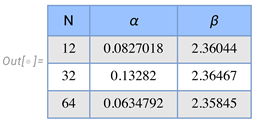
The results of the fitting are tabulated in Table 1. It is apparent that the decay rate is nearly the same for different discretization numbers N. This means that the Sinc-RK method follows the expected error law .
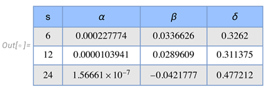
In a second computation, we’ll look at how the global error varies with the number of discretization points N along the RK trajectory. In order to accomplish this, we fix the order s and use (137) to calculate the global error because the Sinc points change along the trajectory. The results of these computations are depicted in Figure 6. We can observe that a power law has a considerable impact on the error in N. The exponential dependency is rather modest and may be mostly ignored (see Table 2). Under this assumption, we observe the well-known error tendency of RK techniques [8]. We can also detect from Figure 6 that s has an exponential dependency as previously discussed. This is seen by the rise in the distance between the computed values.
The results of the fitting in Figure 6 are tabulated in Table 2. It is apparent that the decay rate is almost the same for different approximation orders s. This means that the Sinc-RK method follows the error law where β is a small quantity compared to δ.
In conclusion, the error laws for scalar ODEs follow the error laws of the Sinc methods in a Sinc-RK approximation, resulting in a slightly modified power law for discretization along the trajectory with Sinc points. This suggests the error level is mostly determined by the approximation’s order s.▴
Limit cycles are a feature seen in higher dimensional ODEs [31,32]. In the following example, we will compute a limit cycle for a system of first-order ODEs.
Example 4
(Limit Cycle of a First Order System using L-RK.). Birkhoff and Rota demonstrate that coupled systems of first-order ODEs have stable limit cycles [32]. We extend their model by parameterizing the equations’ major coupling term. This parameter transforms the limit cycle from a rounded square over a circle to a more or less square shape. The limit cycle is a rounded square for , a circle for , but deformed to a diamond for . The underlying differential equations have the following form.
where λ is the coupling parameter and , are the initial conditions. To assess the influence of λ, we adjust the coupling parameter at a predetermined interval. There is no exact solutions to this system of ODEs.
We use the L-RK approach to calculate the limit cycle structure. To do this, we employ the same starting conditions for varying parameters λ to ensure a comparable outcome. The parameters λ are supplied in discrete steps, and the approximants are calculated with the Lagrange Runge-Kutta approach. We set the approximation order s to and the number of discrete points on the trajectory to . The greater order assures a minimal error, and the quantity of discrete points ensures computation stability. We employ orthogonal Chebyshev polynomials to determine the discretization locations.
The computation results are displayed in Figure 7 and Figure 8. Figure 7 depicts the approximants (dots) and Lagrange interpolants (solid lines) for various coupling constants λ. The approximants and interpolants match precisely, resulting in only negligible errors owing to interpolation. We employ Chebyshev polynomials as a basis since similar to Sinc discretization, convergence is better near the interval’s start and end. This is due to the root distribution being relatively near to the interval’s endpoints. We also explored Gegenbauer and Legendre polynomials, which produced tiny oscillations around the ends. Given the identical starting conditions and an increase in the coupling constant λ, the approximants exhibit oscillations after a delay time τ. When λ is raised, a transition zone is generated and the amplitude of the oscillations decrease without damping phenomena. Furthermore, we notice the creation of approximant structures as λ grows. The oscillations’ operating time, τ, rises with λ.
A quasi phase diagram over (Figure 8 left panel) clearly represents the reduction in amplitudes, the distortion of the oscillation, and the delay τ for the commencement of the oscillations. Given the minor errors present, it is evident that limit cycles are emerging. The limit cycles include circular structures for , rounded square structures for , and clear square structures for . We can also notice that the limit cycles for exhibit tiny oscillations in the transient range τ. However, these do not cause instability and are governed by the order s of the approximants and the relatively large number n of discretization points. These oscillations will fade away if we keep increasing s and n. The right panel in Figure 8 depicts a limit cycle created by approximants with varying initial conditions. The coupling constant here is .
Figure 8 (right panel) shows that the center of the phase plane is unstable, whereas the limit cycle is stable.▴
Example 5
(Troesch’s Problem as Initial Value Problem Solved using gL-RK.). First, let us define the problem so that we can assess the relevance of the strategy. Weibel first developed Troesch’s equation while investigating a plasma confinement problem in 1959 [30]. The problem was formulated as a non-linear two point boundary problem (BVP), which Troesch studied one year later [33] in the representation:
with and , where . The inconspicuous problem comprises one parameter λ, which might change in principle in the range . However, the numerical approximation for values presented significant complications [33,37]. This was the starting point for several investigations into the problem, ending in the 1970s with an analytic solution given by Bulrisch, Stoer, and Bulrisch as a toy problem [35,38]. Since then, it is known that the equivalent initial value problem may be addressed using Jacobi elliptic functions. The exact solution to the related Cauchy initial value problem (IVP)
with and , where s is a real value and satisfies . The IVP possesses the exact solution
which is important for testing the numerical approximation in an accurate manner. Stoer and Bulirsch highlighted the relationship between (140) and (141) while discussing shooting approaches for solving BVP utilizing IVP methods [39]. These writers have already pointed out that the BVP has a moveable logarithmic singularity around its upper border. However, they demonstrated that, although being outside the interval , this singularity is caused by cn’s critical behavior at the terminus. In (142), sn and cn are Jacobian elliptic functions of modulus k that depend on the initial slope s. If represents the quarter period of cn, then cn has a zero at
and therefore has a logarithmic singularity there [39]. But has the expansion
or, rewritten in terms of s,
For the solution of the actual boundary-value problem, i.e.,
we require the values of s that depend on the choice of λ. For different λ values, the starting value s is determined by solving (146) with the exact solution in this expression. To solve the equation for s, a high level of precision in the root finding problem is necessary to provide a valid result. All of these relationships are known since Bulrisch and Stoer investigated the topic [35,38].
However, as Troesch [33] and Ehrlich [36] noted, this two-point BVP is numerically unstable and intricate. At approximately the same time, Roberts and Shipman [40] proposed that this problem could only be solved by combining three methods: the perturbation technique, the parallel shooting method, and the continuation method. They suggest that a mix of these strategies is required since none of them alone is effective enough to provide a solution. In fact, their technique only provides valid solutions for equation (140) for . Jones [41] utilized a modified Newton approach to solve this problem. Miele, Aggarwal, and Tietze [42] attempted to apply a modified quasi-linearization approach with limited success. Troesch discovered its numerical solution in [37], utilizing the shooting method. In [46], this problem was solved using the decomposition technique; in [48,49], the variational iteration method was used; in [40], a combination of the multipoint shooting method with the continuation and perturbation technique was applied to the problem; in [42], the quasi linearization method had a limited success; in [43], the method of transformation groups appeared; in [44], the invariant embedding method delivered hardly convincing results; in [45], the inverse shooting was applied and many more. Overall, the methodologies utilized were fairly restrictive and did not result in a definitive numerical procedure. As a result, the problem requires more numerical efforts to be addressed effectively.
We shall apply gL-RK techniques to Troesch’s IVP, demonstrating that a suitable choice of discretization points and the employment of orthogonal polynomials may produce satisfactory numerical results. Using these features correctly can successfully solve Troesch’s problem for a wide variety of λ values. We should point out that Sinc approaches have already been used to solve this problem, albeit with inefficient discretization [47].
To solve the problem (141) numerically as an IVP, we begin with the precise solution (142), which includes the unknown parameter s. If we wish to solve the problem using an IVP, we must first determine the initial slope s. To find s, we use the boundary condition (146) . This boundary condition is transformed into an initial condition by calculating s numerically from the precise solution using the root finding approach for a given λ. We utilize the parameter , which is greater than the number provided in the literature.

This, in turn, yields the exact answer for the specified λ value. We will then use the precise answer as a reference for estimating errors.

To solve the initial value problem numerically, we employ the Jacobi polynomials as a basis for collocation and discretization. Our observations indicate that given the order s, there is a lower constraint at which the Newton method cannot solve the implicit determining equations. Only when this lower threshold is exceeded can a stable solution be achieved. In the following computations, we use as the minimum approximation order. The gL-RK approach is discretized using Jacobi points of size . We use the synchronized variant, with parameters and .
Figure 9 depicts the results of the computations with . The left panel shows the exact solution (solid line), the interpolant (dashed), and the approximant (dots). The numerical approximations are visually indistinguishable from the exact result. The right panel displays the absolute values of local errors for both the interpolant (solid line) and the approximant (dots). The approximant’s discrete error is several orders of magnitude smaller than the interpolant’s local error. However, at times, the interpolant and approximant errors coincide (which is not rectified in this graph).
We solved the approximations for Troesch’s initial value problem using a similar calculating procedure as above, but with the parameter λ variable. The different solutions are illustrated in Figure 10. The related local errors have the same order of magnitude as in Figure 9. The graphs in Figure 10 indicate that the function y rises extremely quickly as t approaches 1 for larger λ. The shift in slope grows steeper as λ increases. The gL-RK technique efficiently handles the fast expansion of the function y, even with small values for approximation order and RK number of support points . We employed Jacobi polynomials for both interpolation and discretization.
The example demonstrates how the gL-RK approach may be used to efficiently compute a reasonably stiff problem such as the Troesch equation.▴
Example 6
(The nonlinear Klein-Gordon Equation Solved using gL-RK.). In this example, we will provide a solution technique for nonlinear partial differential equations (nPDE) that is based on Lie’s method of infinitesimal transformations [50] and use the gL-RK method for numerical solution. This method enables us to convert the PDE to an ODE and construct the resulting initial value problem. We shall demonstrate this with the cubic Klein-Gordon (cKG) equation.
The cubic Klein-Gordon equation is well known and can be written as
where α and β are real parameters. The determination of infinitesimal symmetries (Lie symmetries) reveals the following transformation under which equation (147) stays invariant
Here the parameters with are group constants which can be freely chosen. The choice of these parameters selects a transformation group under which (147) will be invariant. In addition this selection allows to reduce the nPDE to a nonlinear ODE which solves equation (147).
Selecting the sub-group , , and ; i.e. translations in spatial and temporal variables, we are able to generate via a Lie reduction the following ODE
where . It is straight forward to solve this ODE as an initial value problem with , by selecting and and ; here . The exact solution using the given initial values is .
Since our target is the solution of the boundary value problem (147) with and for , we will use . This allows us to approximate the natural boundary conditions at by values at and in the following setup of the initial value problem in the reduced variable .
Note this definition is possible because we are looking for moving wave solutions of the problem. The application of the gL-RK method to the “initial” value problem delivers the approximant. We should remark, that the initial point of integration is different from zero.
Figure 11 shows the gL-RK calculation results for u and . The left panel displays the exact solution (solid line), the interpolant (dashed), and the approximant (dots). Figure 11’s right panel displays the absolute local error for u as well as the absolute local error of the approximant (dots). With a small number of steps in the RK technique and an approximation order of , we reach a global error of . For practical applications, this is enough to derive the solution structure.
When ζ is substituted by the dependency in x and t; , the similarity solution yields the solution to the boundary value problem. Figure 12 illustrates the wave’s form as a simple solitary peak, as well as its derivative. We see that the basic peak travels at a constant speed .
When we vary the cubic Klein-Gordon equation’s parameters α and β and adjust the initial conditions, we get an oscillating wave in space and time. The used initial conditions are , on the interval . The parameters are set to , , and .
Again we use the gL-RK approach to recalculate the approximant and interpolant for this initial value problem using and RK steps. Jacobian polynomials are used to define the basis and discretize the data.
Figure 13 shows the results. The solution’s structure is periodic in both u and . This is clearly a nonlinear solution, as the minima and maxima of u are rather sharply curved, and the derivatives are flatter at their extrema. The right panel of Figure 13 displays a phase-space picture that clearly depicts the solution’s periodicity.
If we return from the similarity variable to the spatial and temporal coordinates (see Figure 14), the wave formation can be represented in an coordinate system. The tilting of the wave crests in this coordinate system is attributable to the finite velocity v. However, it is obvious that the wave nature occurs in the spatiotemporal continuum, but only a limited range can be represented by the finite integration with the gL-RK method.
In conclusion, the gL-RK approach, when paired with the Lie symmetry method, produces useful results for partial differential equations. This necessitates reframing a boundary-value problem as an initial value problem. We understand that this is not always practicable, but when combined, it may result in significant time and resource savings.▴
7. Conclusions
The technique of implicit Runge-Kutta procedures shows that, using the collocation method and therefore the representation of the matrix and the weights , a well-defined algorithm exists for determining a numerical implicit Runge-Kutta process. The many representations of the matrix generate variability, allowing for tailored adaptation to a given problem. This technique works for both stiff and non-stiff initial value problems. In addition to numerical integration, comprehending the matrix enables direct comments about the method’s stability when the pole and zero distributions of the stability function are analyzed.
The method’s stability may be graphically evaluated using proven methods like order stars. Our numerical investigations demonstrated that parameter-independent orthogonal polynomials are not restricted in stability. This is an open problem for parameter-dependent orthogonal polynomials when the number of parameters is greater than one. For example, for Gegenbauer polynomials , there is an upper constraint in m that is smaller than . We discovered both a variable upper bound and a fixed lower bound at . Additionally, there are no restrictions for orders . The upper bound was estimated with a rational expression and a Thiele continued fraction. The approximant approaches the fixed value for . The interval for stable L-RK techniques using Gegenbauer polynomials is provided by for and for .
The approach presented is simple to implement and highly efficient in numerical calculation. Furthermore, the strategy based on Sinc approximations has the well-known feature of exponential convergence. The zeros of orthogonal polynomials are sensitive in the classes of resultant functions, allowing for a priori estimate of the global error. It is also critical that a priori error formulae exist for calculating the global error, allowing automated computation by defining error tolerances. An a posteriori additional error analysis is obsolete.
The examples provided demonstrate that implicit RK techniques based on indefinite integrals provide an approach that is highly adaptable while requiring little implementation work. The main idea is that just the matrix and the weights must be known. Thus, the procedure is specified using a Butcher table. The variability derives from the discrete representation of indefinite integrals, which may be obtained using orthogonal polynomials or Sinc techniques.
Acknowledgments
We appreciate having productive talks on this topic with Frank Stenger, who passed away untimely in 2024.
Conflicts of Interest
There are no conflicts of interest.
References
- Butcher, J.Ch. Numerical methods for ordinary differential equations; John Wiley & Sons, Chichester, West Sussex, United Kingdom, 2016.
- Stenger, F. Numerical Methods Based on Sinc and Analytic Functions; Springer New York, New York, NY, 1993.
- Stenger, F. Handbook of Sinc Numerical Methods; CRC Press, Boca Raton, 2011.
- Baumann, G. New Sinc Methods of Numerical Analysis; Springer, Cham, 2021.
- Runge, C. Über die numerische Auflösung von Differentialgleichungen. Math. Ann., 1895, 46, 167-178.
- Kutta, W. Beitrag zur näherungsweisen Integration totaler Differentialgleichungen. Z. Math. Phys. 1901, 46, 435-453.
- Hairer, E. Solving Ordinary Differential Equations. 1: Non-stiff Problems; Springer, Berlin Heidelberg, 2009.
- Hairer, E.; Wanner, G. Solving Ordinary Differential Equations. 2: Stiff and Differential Algebraic Problems. Springer, Berlin Heidelberg, 2010.
- Guillou, A.; Soulé, J.L. La résolution numérique des problèmes différentiels aux conditions initiales par des méthodes de collocation. Revue française d’informatique et de recherche opérationnelle. Série rouge, 1969, 3(R3), 17-44 .
- Wright, K. Some relationships between implicit Runge-Kutta, collocation and Lanczos τ methods, and their stability properties. BIT Numerical Mathematics, 1970, 10, 217-227.
- Gautschi, W. Numerical Analysis. 2nd ed Springer / Birkhäuser, New York, 2012.
- Schmeisser, G.; Stenger, F. Sinc Approximation with a Gaussian Multiplier. Samp. Th. Sig. Im. Proc., 2007, 6, 199-221.
- Stenger, F. Collocating convolutions. Math. Comp., 1995, 64, 211-235.
- Shen, X.; Zayed, A.I. Multiscale signal analysis and modeling. Improved Approximation via Use of Transformations. Springer, New York, NY 2013, 25-49.
- Han, L.; Xu, J., Proof of Stenger’s conjecture on matrix of Sinc methods. Journal of Computational and Applied Mathematics, 2014, 255, 805--811.
- Gray, R.M. Toeplitz and circulant matrices. A review. Now Publishers, Boston 2006.
- Trench, W.F. Spectral Evolution of a One-Parameter Extension of a Real Symmetric Toeplitz Matrix. SIAM. J. Matrix Anal. & Appl., 1990, 11, 601-611.
- Grenander, U.; Szegö, G. Toeplitz forms and their applications. American Mathematical Society, Providence, R.I. 2001.
- Gautschi, W. Orthogonal polynomials: computation and approximation. OUP Oxford, 2004.
- Olver, F.W.J. ed. NIST handbook of mathematical functions hardback and CD-ROM. Cambridge University Press, 2010.
- Aitken, A.C. On interpolation by iteration of proportional parts, without the use of differences. Proceedings of the Edinburgh Mathematical Society 1932, 3, no. 1, 56-76.
- Neville, E.H. Iterative interpolation. St. Joseph’s IS Press, 1934.
- Mühlbach, G. The general Neville-Aitken-algorithm and some applications. Numerische Mathematik, 1978, 31, no. 1, 97-110.
- Occorsio, D.; Russo. M. G. A new quadrature scheme based on an Extended Lagrange Interpolation process. Applied Numerical Mathematics 2018, 124, 57-75.
- Moalemi, Z. A Generalization of Lagrange Interpolation and Its Applications, PhD Thesis, K.N.Toosi University of Technology, Tehran, Iran, 2018.
- Cheney, W.; Light, W. A course in approximation theory. Vol. 101. American Mathematical Society, 2009.
- Karlin, S.; Studden, W.J. Tchebycheff Systems: With Applications in Analysis and Statistics, Pure Appl. Math. 15, Interscience Publishers John Wiley & Sons, New York, 1966.
- Dahlquist, G.G. A special stability problem for linear multistep methods. BIT Numerical Mathematics, 1963, 3(1), 27-43.
- Ehle, B. On Padé Approximations to the Exponential Function and A-Stable Methods for the Numerical Solution of Initial Value Problems, PhD, Waterloo, 1969.
- Weibel, E. On the Confinement of a Plasma by Magnetostatic Fields, Physics of Fluids, 1959, 2, 1, 52-56.
- Bender, C. M.; Orszag, S. A. Advanced Mathematical Methods for Scientists and Engineers I: Asymptotic Methods and Perturbation Theory, 1st ed, Springer New York, New York, 1999.
- Birkhoff, G.; Rota, G.-C. Ordinary Differential Equations, 4th ed Wiley, New York, 1989.
- Troesch, B. A. Intrinsic Difficulties in the Numerical Solution of a Boundary Value Problem, Internal Report NN - 142, TRW Inc., Redondo Beach, Calif., 1960.
- Baumann, G.; Stenger, F. Applied Sinc Approximations: Polynomial and Sinc Methods for Solving Calculus Problems in Mathematica, Springer, New York, 2026.
- Stoer, J.; Bulrisch, R. Einführung in die Numerische Matematik, Vol. II, Heidelberger-Taschenbuch 114, Chap. VII, p. 114. Springer-Verlag, Berlin, 1973.
- Ehrlich, L. Experience with Numerical Methods for a Boundary Value Problem, Internal Report NN-141, TRW Inc., Redondo Beach, Calif., 1960.
- Troesch, B. A. A Simple Approach to a Sensitive Two - Point Boundary Value Problem, Journal of Computational Physics, 1976, 21, 3, 279-290.
- Bulrisch, R. Die Mehrzielmethode zur Numerischen Losung von Nichtlinearen Randwertproblemen und Aufgaben der Optimalen Steuerung, Vortrag im Lehrgang Flugbahnoptimierung der Carl Cranz-Gesellschaft E. V., October 1971.
- Stoer, J.; Bulirsch, R. Introduction to numerical analysis. Springer, New York, NY, 2002.
- Roberts, S.; Shipman, J. On the Closed form Solution of Troesch’s Problem, Journal of Computational Physics, 1976, 21, 3, 291-304.
- Jones, D. J. Solution of Troeschs, and other, two point boundary value problems by shooting techniques, Journal of Computational Physics, 1973, 12, 3, 429-434.
- Miele, A.; Agarwal, A.; Tietze, J. Solution of Two-Point Boundary-Value Problems with Jacobian Matrix Characterized by Large Positive Eigenvalues, Journal of Computational Physics, 1974, 15, 2, 117-133.
- Chiou, J.; Na, T. On the Solution of Troesch’s Non-linear Two-Point Boundary Value Problem Using an Initial Value Method, Journal of Computational Physics, 1975, 19, 3, 311-316.
- Scott, M. On the Conversion of Boundary-Value Problems into Stable Initial-Value Problems via Several Invariant Imbedding Algorithms, In: A. K. Aziz, Ed., Numerical Solutions of Boundary-Value Problems for Ordinary Differential Equations, Academic Press, New York, 1975, 89-146.
- Snyman, J. Continuous and Discontinuous Numerical Solutions to the Troesch Problem, Journal of Computational and Applied Mathematics, 1979, 5, 3, 171-175.
- Deeba, E.; Khuri, S.; Xie, S. An Algorithm for Solving Boundary Value Problems, Journal of Computational Physics, 2000, 159, 2, 125-138.
- El-Gamel, M.; Sameeh, M. A Chebychev Collocation Method for Solving Troesch’s Problem, International Journal of Mathematics and Computer Applications Research, 2013, 3, 2, 23-32.
- Khuri, S. A. A Numerical Algorithm for Solving Troeschs Problem, International Journal of Computer Mathematics, 2003, 80, 4, 493-498.
- Chang, S. A Variational Iteration Method for Solving Troesch’s Problem, Journal of Computational and Applied Mathematics, 2010, 234, 10, 3043-3047.
- Baumann, G. Symmetry Analysis of Differential Equations with Mathematica, Springer New York, New York, NY, 2000.
- Iserles, A.; Nørsett, S. P. Order Stars, 1. ed Chapman and Hall, London, 1991.
- Brezinski, C. Padé-Type Approximation and General Orthogonal Polynomials, Birkhäuser Basel: Imprint: Birkhäuser, Basel, 1980.
- Brezinski, C.; Redivo Zaglia, M. Extrapolation Methods: Theory and Practice, North-Holland Distributors for the U.S. and Canada, Elsevier Science Pub. Co, Amsterdam New York, N.Y., 1991.
- Brezinski, C. Extrapolation and Rational Approximation: The Works of the Main Contributors, Springer International Publishing AG, Cham, 2020.
- Ait-Haddou, R.; Alselami, H. The Stenger conjectures and the A-stability of collocation Runge-Kutta methods. Journal of Inequalities and Applications, 2023, 107. [CrossRef]
Figure 1.
Order stars for a Padé approximation of . The zeros (•) and poles (★) are displayed, together with the absolute value of is represented by the colors red for 1 and blue for 0.
Figure 1.
Order stars for a Padé approximation of . The zeros (•) and poles (★) are displayed, together with the absolute value of is represented by the colors red for 1 and blue for 0.
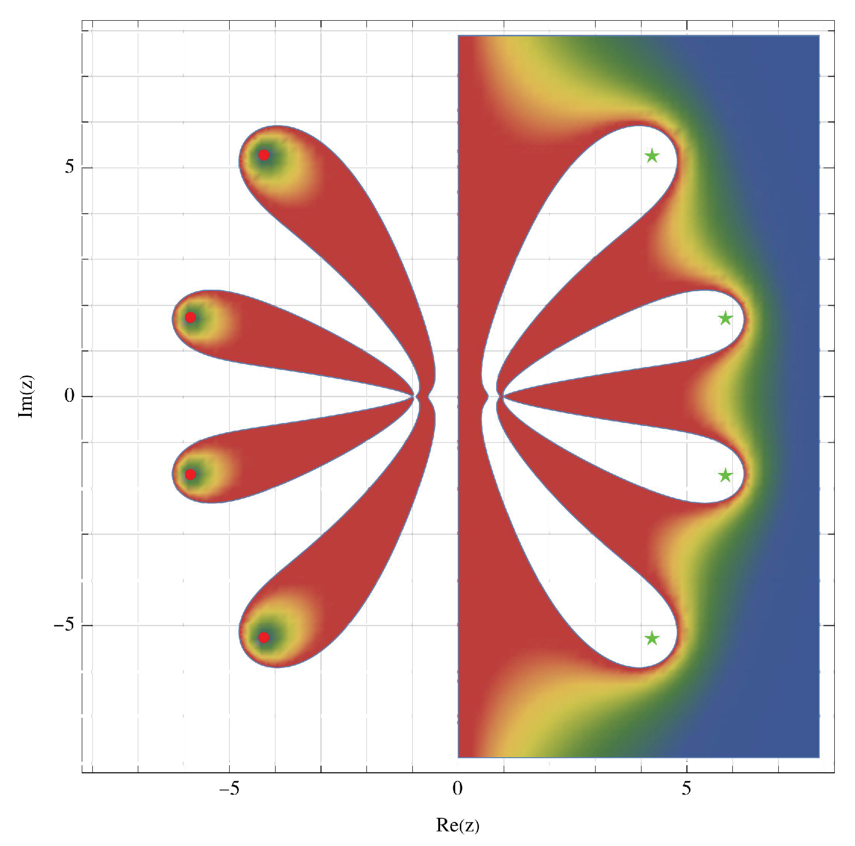
Figure 2.
The Padé approximation of the Dahlquist problem is based on Gegenbauer polynomials with in each column from left to right as basis. Discretization uses Legendre , Chebyshev , and Chebyshev from left to right columns, with from top to bottom in each row.
Figure 2.
The Padé approximation of the Dahlquist problem is based on Gegenbauer polynomials with in each column from left to right as basis. Discretization uses Legendre , Chebyshev , and Chebyshev from left to right columns, with from top to bottom in each row.
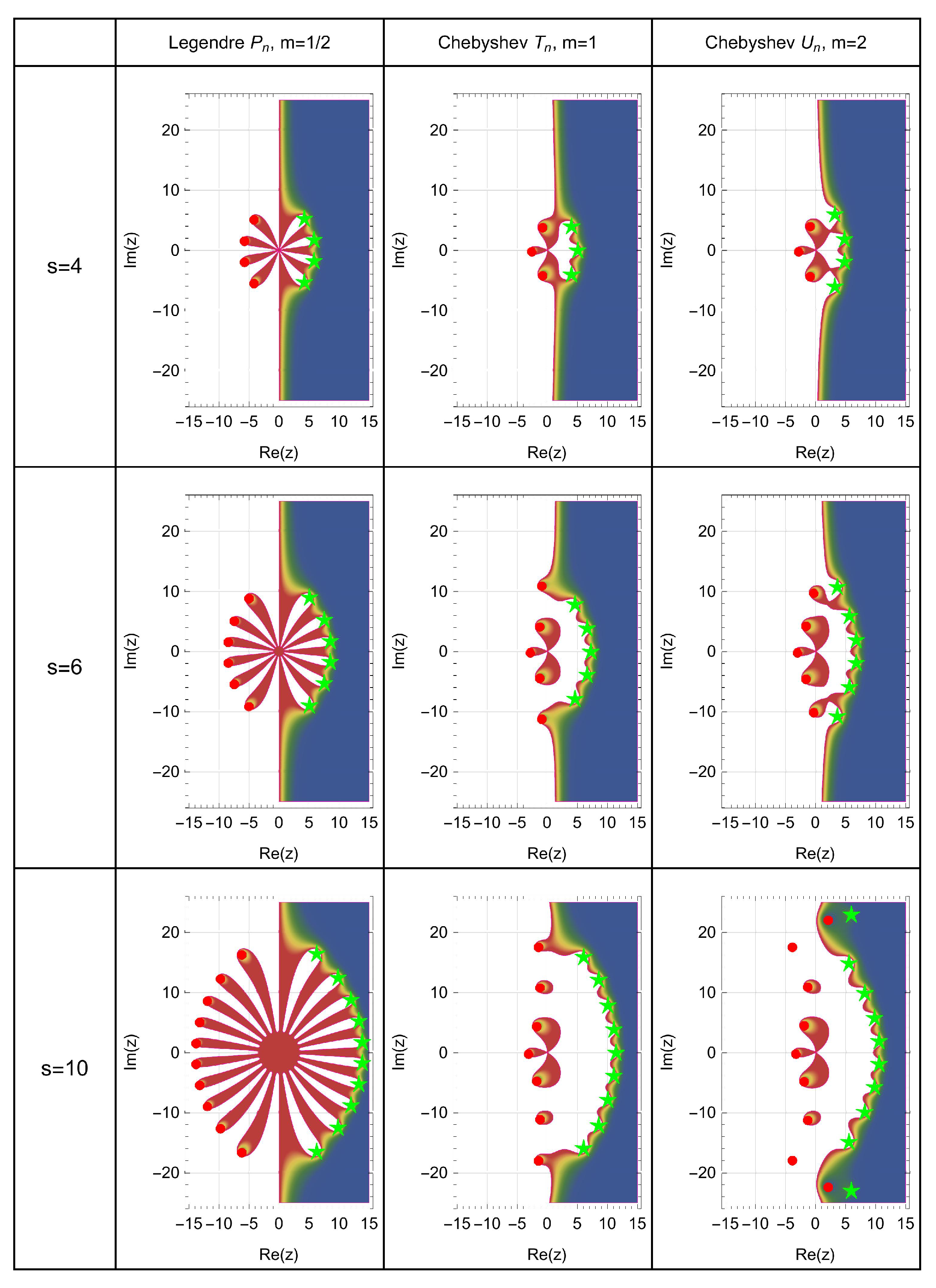
Figure 3.
Comparison of symbolic and analytic solutions to a first-order ODE with initial conditions . The left panel displays the halved component of the Gaussian function . Dots indicate the discrete Sinc-RK solution. The solid line depicts the symbolic solution, whereas the dashed line reflects the Sinc interpolation of the Sinc-RK findings. The right panel’s local error depicts the interpolation error (solid line) as well as the discrete Sinc-RK approximation with an order of and Sinc points in the RK iteration.
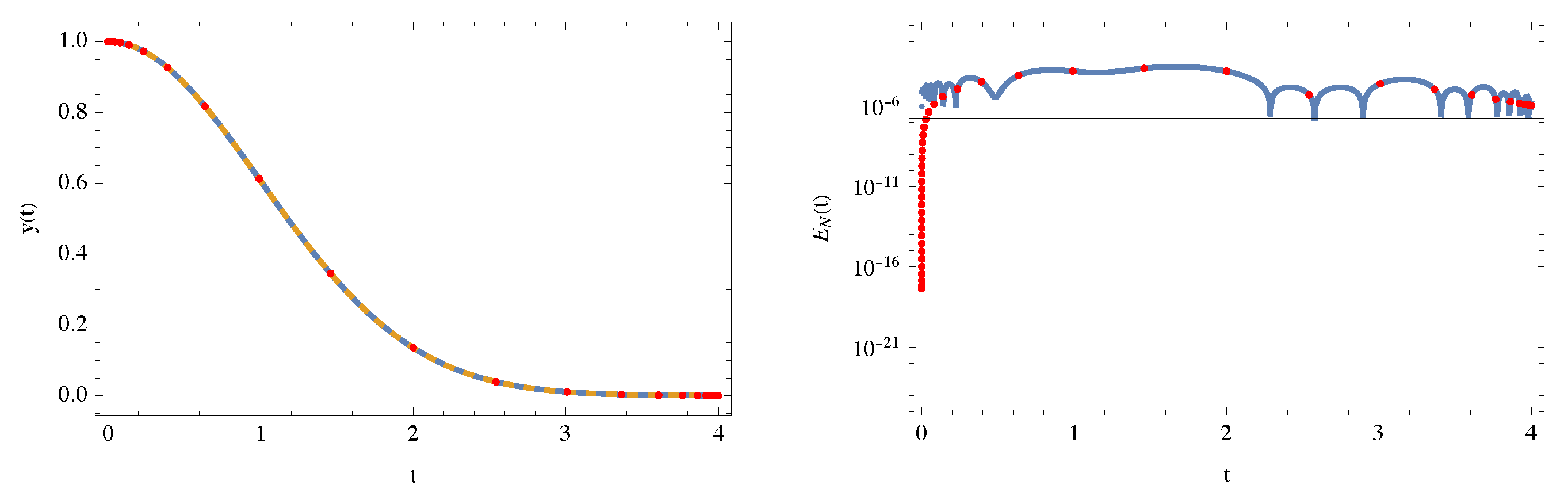
Figure 4.
Comparison of symbolic and analytic solutions to a first-order ODE with initial conditions . The left panel displays the halved component of the Runge function . Dots indicate the discrete Sinc-RK solution. The solid line depicts the symbolic solution, whereas the dashed line reflects the Sinc interpolation of the Sinc-RK findings. The right panel’s local error depicts the interpolation error (solid line) as well as the discrete Sinc-RK approximation with an order of and Sinc points in the RK iteration.
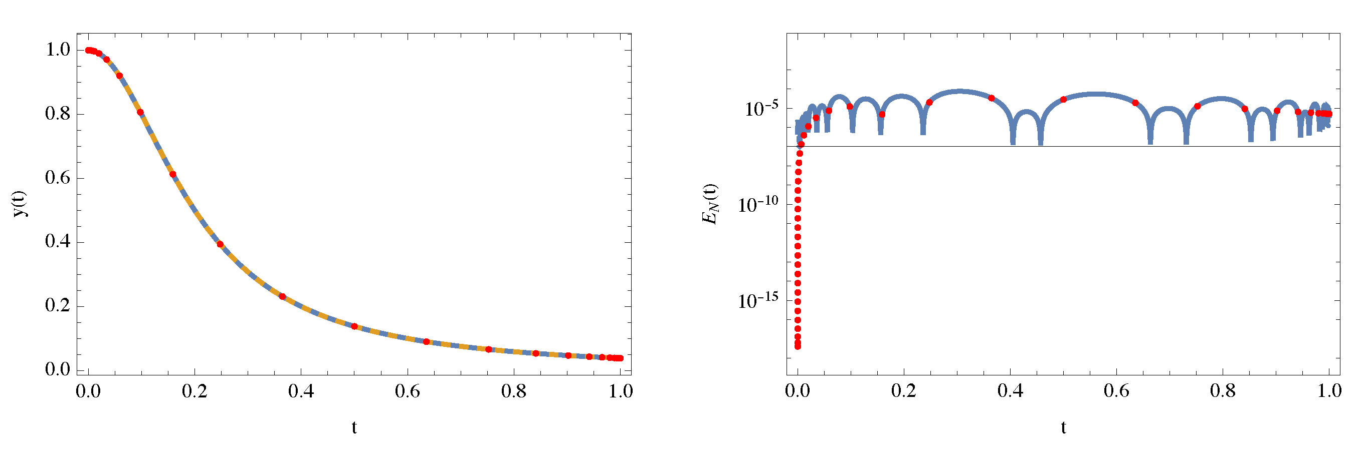
Figure 5.
The global error’s decay in a Sinc-RK technique as a function of the approximation order s. The variation of the Sinc score N is the number of Sinc discretization points.
Figure 5.
The global error’s decay in a Sinc-RK technique as a function of the approximation order s. The variation of the Sinc score N is the number of Sinc discretization points.
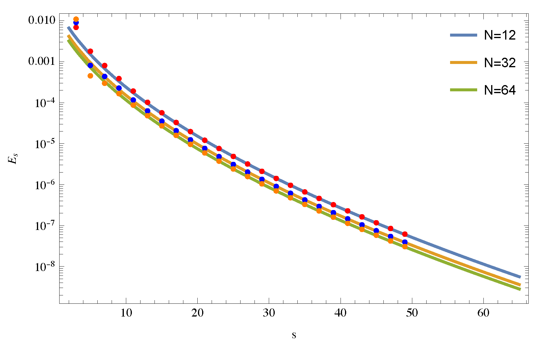
Figure 6.
The error’s decay in a Sinc-RK technique as a function of the discretization steps N. The variation of the approximation order s is indicated in the plot legend.
Figure 6.
The error’s decay in a Sinc-RK technique as a function of the discretization steps N. The variation of the approximation order s is indicated in the plot legend.
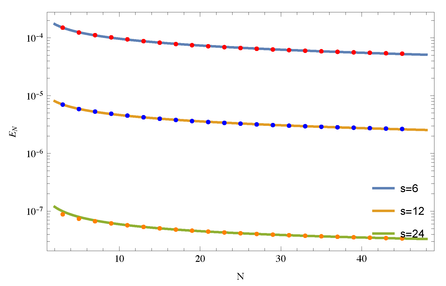
Figure 7.
Approximants of system (139) and (138) for different coupling parameters . Initial conditions are and .
Figure 7.
Approximants of system (139) and (138) for different coupling parameters . Initial conditions are and .
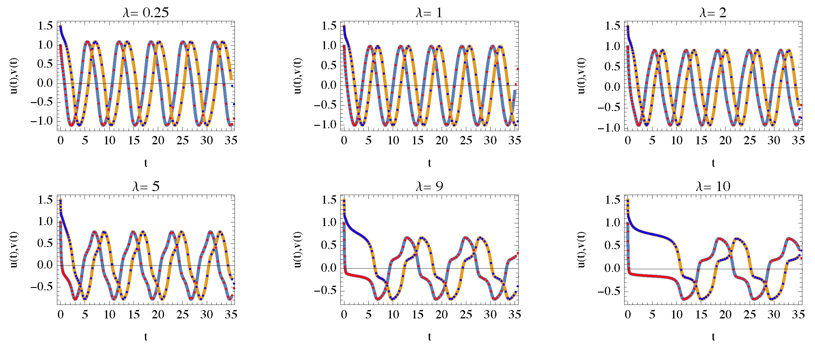
Figure 8.
Limit circles on the “phase plane” with fixed initial conditions and variable coupling constants (left panel). The right panel depicts a limit cycle with under various initial conditions.
Figure 8.
Limit circles on the “phase plane” with fixed initial conditions and variable coupling constants (left panel). The right panel depicts a limit cycle with under various initial conditions.
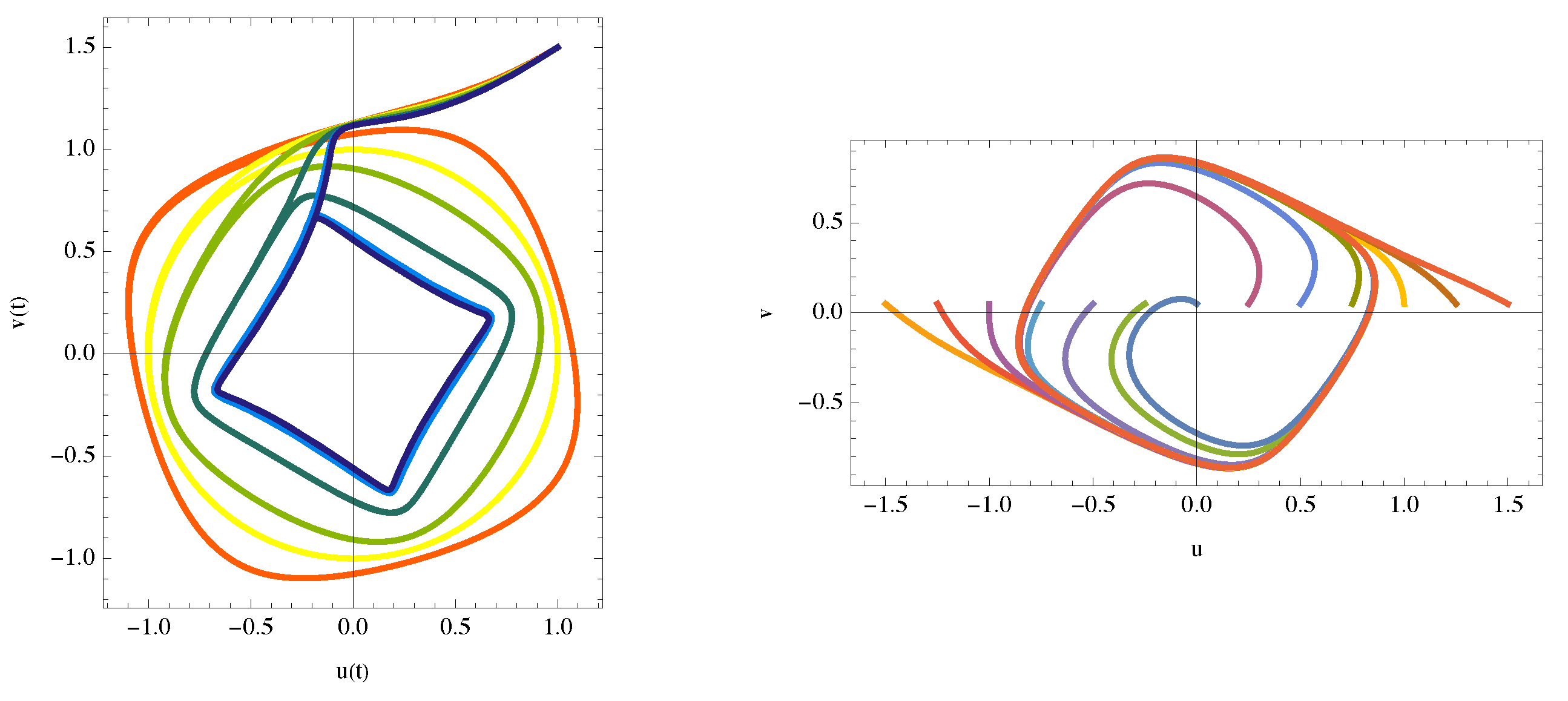
Figure 9.
Troesch’s BVP is solved using the IVP technique and the gL-RK method. The approximation uses a Jacobi basis and discretization with and .
Figure 9.
Troesch’s BVP is solved using the IVP technique and the gL-RK method. The approximation uses a Jacobi basis and discretization with and .
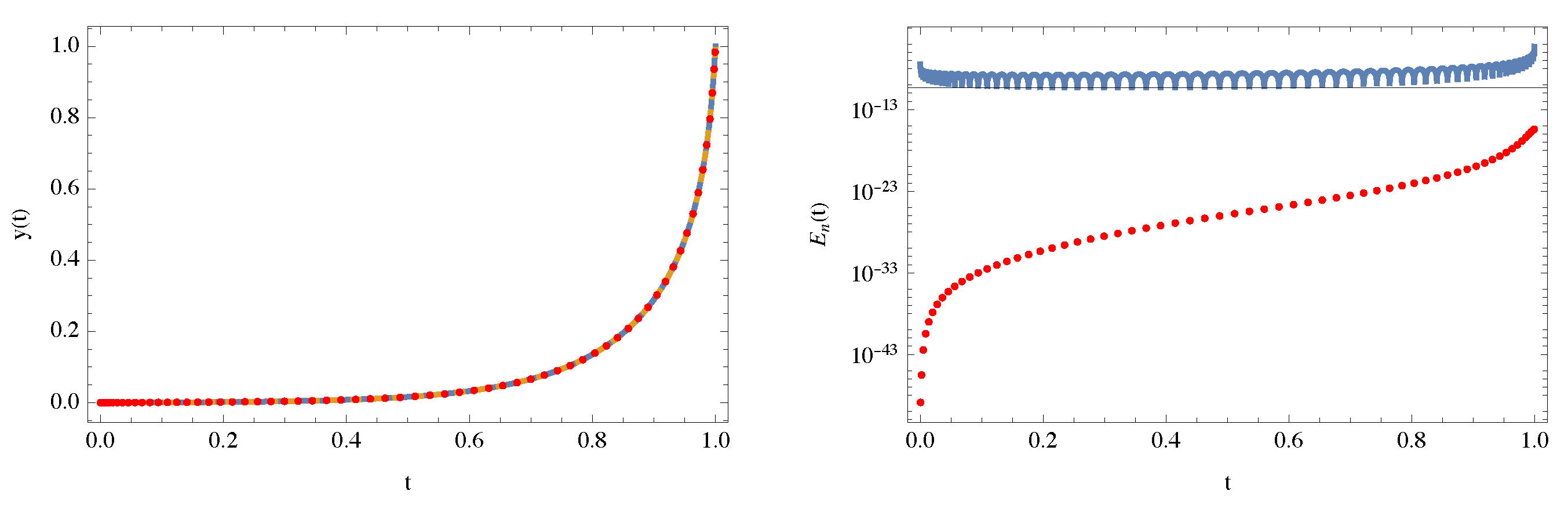
Figure 10.
Troesch’s BVP solutions for different values of .
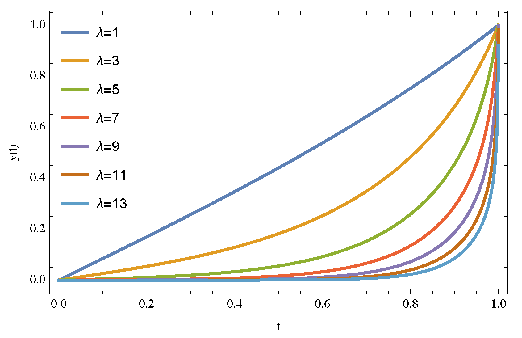
Figure 11.
Similarity solution to the cubic Klein-Gordon equation.
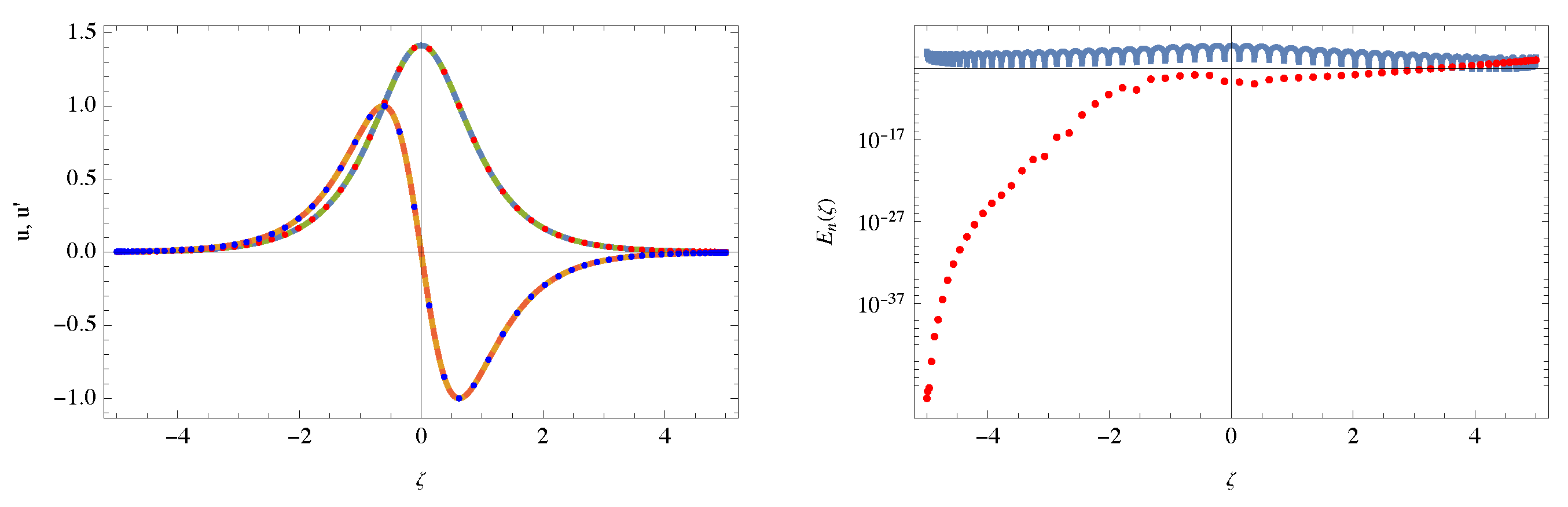
Figure 12.
Solitary wave solution to the cubic Klein-Gordon equation.
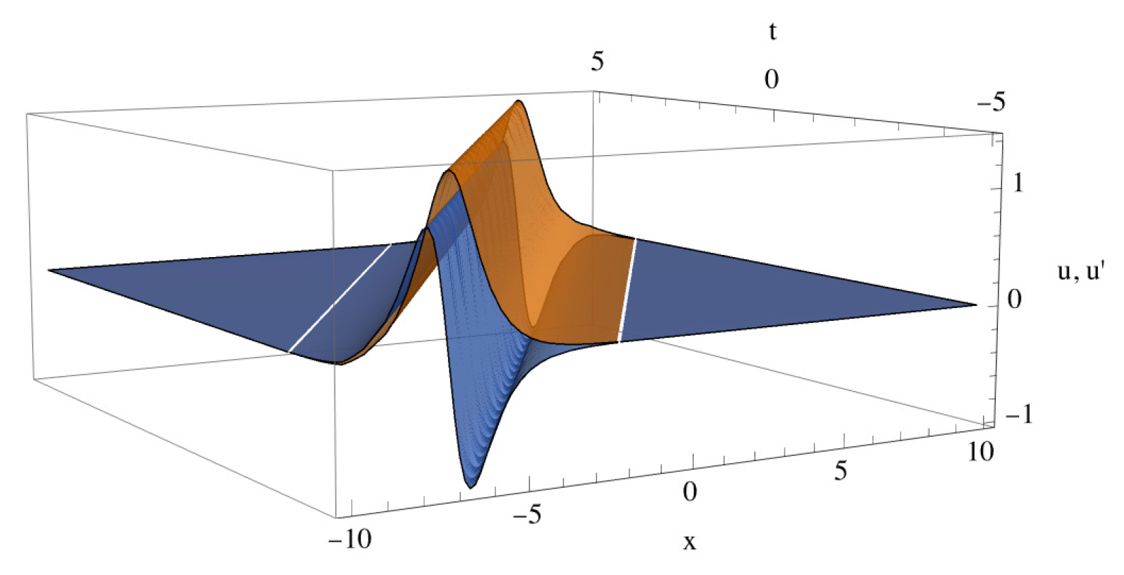
Figure 13.
Periodic wave solution to the cubic Klein-Gordon equation.
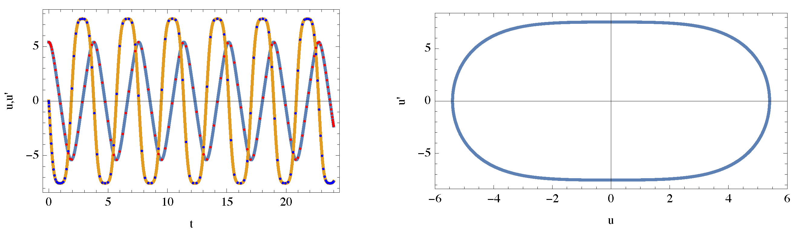
Figure 14.
3D periodic wave solution to the cubic Klein-Gordon equation.
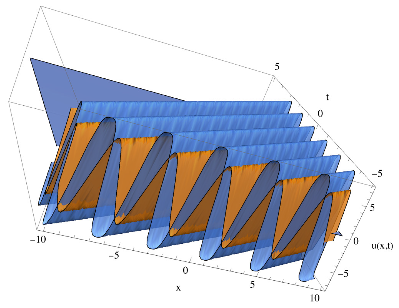

Table 1.
For various discretization N of the Sinc-RK approximation, the global error parameters in are given to indicate the decay rate for various approximation orders s.
Table 1.
For various discretization N of the Sinc-RK approximation, the global error parameters in are given to indicate the decay rate for various approximation orders s.
 |
|---|
Table 2.
For various approximation orders s of the Sinc-RK approximation, the global error parameters in are given to indicate the decay rate for various approximation orders s.
Table 2.
For various approximation orders s of the Sinc-RK approximation, the global error parameters in are given to indicate the decay rate for various approximation orders s.
 |
|---|
Disclaimer/Publisher’s Note: The statements, opinions and data contained in all publications are solely those of the individual author(s) and contributor(s) and not of MDPI and/or the editor(s). MDPI and/or the editor(s) disclaim responsibility for any injury to people or property resulting from any ideas, methods, instructions or products referred to in the content. |
© 2026 by the authors. Licensee MDPI, Basel, Switzerland. This article is an open access article distributed under the terms and conditions of the Creative Commons Attribution (CC BY) license (http://creativecommons.org/licenses/by/4.0/).
Copyright: This open access article is published under a Creative Commons CC BY 4.0 license, which permit the free download, distribution, and reuse, provided that the author and preprint are cited in any reuse.