

Submitted:
19 March 2026
Posted:
19 March 2026
You are already at the latest version
Abstract
We present a numerical study of high frequency acoustic wave scattering from two types of rigid scatterers, a circular disk and a red blood cell (RBC) shaped (biconcave) obstacle. Using an iterative frequency domain solver, we compute the steady state pressure and energy density distribution. The sound speed varies inside the source 1350 m/s and 1650 m/s with ambient medium 1500 m/s. Simulations are performed at frequencies up to 366 MHz. Results are sampled along the center line through the source center for direct comparison. Both solver produce nearly identical pressure amplitude profile, with a pronounced central pressure maximum and decaying oscillations toward the edges. As frequency increases, the number of concentric interference rings around the source grows, and the central lobe narrows (for RBC). The number of iterations required for convergence rise sharply with frequency. The simulations capture the expected wave phenomena and demonstrate that the Convergent Born series (CBS) solver remains reliable and robustness for strong scattering contrasts in presence of spatially adaptive preconditioner.
Keywords:
acoustic scattering
; red blood cell
; convergent Born series
; steady state
; adaptive preconditioner
1. Introduction
Modeling high-frequency acoustic wave scattering in heterogeneous media is important for applications like medical ultrasound, acoustic imaging, and materials characterization. For example, intravascular and small-animal ultrasound systems routinely operate above 20–30 MHz, where individual red blood cells (RBCs) and other microstructures strongly influence the backscattered signal [1]. In this non-Rayleigh regime (e.g., 73.2 MHz in our study), the exact shape of a scatterer – such as the biconcave geometry of an RBC – can significantly alter the acoustic field. In order to predict these fields, one must solve the Helmholtz equation for the pressure field in a fluid with embedded objects. Direct time-domain simulation (followed by Fourier analysis) is one approach, but it can be prohibitively expensive and inaccurate at high frequencies due to long runtimes and dispersion error. Similarly, naive direct solvers of the frequency-domain equation require large memory. As a result, fast frequency-domain methods have attracted attention. In particular, iterative Born-series solvers can efficiently handle large Helmholtz problems by summing successive scattering interactions. The CBS method is a preconditioned Born-series formulation that guarantees convergence even for strong scatterers [2]. Recent work has shown that a first-order, matrix-free Born-series solver (using FFTs and a special split-preconditioner) can compute pressure and velocity fields efficiently with minimal memory.
In this paper, we apply such an iterative solver to study acoustic scattering by two distinct rigid scatterers in 2D: (1) a circular disc and (2) an idealized red blood cell (RBC)–shaped biconcave plate. Key physical parameters are chosen to mimic strong scattering: the scatterer has an internal sound speed of 1650 m/s while the outside fluid has the speed of a typical fluid. We focus on monochromatic plane-wave excitation at frequencies around 73.2 MHz, so that the nondimensional size parameter ka is on the order of unity to several (where a is radius).
Our numerical approach is a frequency-domain Helmholtz solver based on the Convergent Born Series. The algorithm iteratively updates the pressure field using FFT-based convolution and a “universal split” preconditioner, avoiding any large matrix inversions. We also compare it to a reference solution (RS) to verify accuracy. Both methods operate in a matrix-free fashion: at each step the scattered field is computed via fast Fourier transforms without constructing the full system matrix. This framework is capable of handling the strong density/sound-speed contrast we impose.
Frequency dependence: As expected, higher frequency (shorter wavelength) produces more concentric interference fringes in the pressure field around the scatterer. The number of rings visible in the spatial pressure map increases with frequency, and the central beam width narrows. This is consistent with wave optics: finer features emerge when ka grows. Shape effects: The biconcave (RBC) scatterer yields a noticeably narrower central pressure lobe than the simple circular disk, even though the total number of rings is similar. This agrees with prior theoretical work showing that RBC geometry becomes important above 20 MHz. In other words, the disk and RBC of the same effective size scatter differently due to shape. Solver performance: Both the RS and CBS solvers produced nearly identical pressure fields at convergence, validating the implementation. The CBS-based solver converged reliably for our strong-contrast case. However, the number of iterations required grew rapidly at higher frequencies, reflecting the known fact that larger wavenumbers (and stronger contrasts) slow down Born-series convergence.
Overall, the FFT-based solver proved efficient and accurate for this 2D scattering problem. Despite these promising results, there are limitations to note. Our simulations assume an ideal, two-dimensional free-field (non-viscous) environment and rigid (sound-hard) obstacles. In reality, ultrasound waves in tissues would experience absorption and 3D propagation, and actual RBCs may deform or have viscoelastic properties. Future work will extend this framework to three-dimensional geometries, include absorption and more realistic boundary conditions, and consider ensembles of scatterers (e.g., blood suspensions). Experimental validation (for example using micrometer-scale scatterers in water) would also help confirm the predicted scattering patterns. Overall, this study provides a detailed computational exploration of how scatterer shape and frequency influence the acoustic pressure field and demonstrates the capability of modern Born-series solvers in handling high-frequency, high-contrast wave problems.
2. Materials and Methods
2.1. PA Model
In the PA effect, optical absorption produces a localized temperature rise in the medium. This temperature increase causes the medium to undergo thermal expansion. However, the surrounding medium restricts this expansion, resulting in the generation of a thermoelastic pressure rise. This pressure rise subsequently propagates through the medium as an acoustic wave can be expressed as [3,4,5,6],
where denotes the thermoelastic pressure rise, is the volumetric thermal expansion coefficient of the medium. K (RBC, Pa) [3] represents the bulk modulus, and is the temperature increase caused by optical energy absorption. When the conditions of thermal and stress confinement hold, the resulting PA pressure in a homogeneous and non-viscous acoustic medium can be formulated with thermal diffusion time by the following equation [3],
where is the specific heat capacity at constant pressure, is the speed of sound inside the source, and heat deposition function per unit time and volume. To obtain the time-independent form, we assume a time-harmonic dependence of the acoustic field and the heat source. Therefore, the temporal variation of the field can be written as [4],
where and are the wave number within the source and ambient medium. The subscripts s and f state the source (RBC) and the ambient (plasma) medium. is the angular frequency of the incident laser source and incidendent beam intensity with optical absorption coefficient .
2.2. Reference Solution (RS) Method
The RS method provides an analytical benchmark for validating numerical approaches. In this method the governing PA wave equation is solved analytically for a simple geometry by applying appropriate boundary conditions at the interface between the absorbing object and the surrounding fluid. For a cylindrically symmetric configuration, the acoustic field can be expressed in term of cylindrical wave function. The analytical solution is obtained by solving the Helmholtz equation inside and outside the particle while enforcing the continuity of acoustic pressure and normal component of the particle velocity at the boundary. As a result, the acoustic fields are represented by Bessel functions inside the particle and Hankel functions in the surrounding medium. Following this approach, the frequency domain solutions for the PA field inside and outside the cylindrical symmetry are given by [7],
where and , The notations J and represent the Bessel and Hankel function of first kind. These expressions serve as a RS method for comparision with numerical results obtained from Lippmann-Schwinger scattering series (CBS) based methods. The detailed derivation are shown in Appendix A.
2.3. Evans–Fung RBC Model Equation
The geometric shape of a RBC is commonly described by the Evans-Fung model, which represents the chracteristic biconcave structure of the cell. In the present study, the two-dimensional cross-section of the RBC is modeled. The thickness profile of the RBc along the radial direction is given by [8],
where denotes the radial coordinate measured from the cell center and is the half thickness of the RBC. The parameter corresponds to the cell radius, and D is the RBC diameter. The coeffients , , and determine the biconcave profile and are obtained from the geometric parameters of the cell. These parameters are defined as , , , where d denotes the diameter of the central dimple and h represents the maximum height of the RBC rim as shown in Figure 1. The coefficients are then expressed as, , , . For the numerical simulations, the geometric parameters of the RBC are taken as m, , m, m, where t denotes the minimum thickness at the center of the cell. . These parameters produce the typical biconcave morphology observed in healthy human RBCs.
2.4. Lippmann-Schwinger Scattering Series
The time-independent PA wave pressure field at point with opto-acoustic source satisfies the Helmholtz equation [9],
where, source term , sacttering potential and is the real positive number. After inserting the source term and the potential function, the opto-acoustic field inside and outside the source region satisfies the following governing equation,
The solution in the form of volume integral over all the space ( or ) of the PA wavefield expressed as (Morse 1953),
The Green’s function satisfies the inhomogeneous Helmholtz equation with Dirac delta source , which represents the reponse of the medium to a unit point excitation located at .
Again, the differential Equation (6) can be transformed into an equvalent integral equation of the Lippmann-Schwinger type [10],
where and are the Green’s function and the PA wave field in the background medium over the space where . For a three dimensional, the Green’s function corresponds to a spherical wave that decays inversely with distance from the source. In a two dimensional domain, the solution is expressed in terms of the Hankel function of the first kind, which represents cylindrical wave propagation. In contrast, the one dimensional form corresponds to a pair of propagating plane waves traveling away from the source location. In In three different dimensions, the free space Helmholtz Green’s function can be written as [11],
For the numerical implementation Equation (10) is discretized on a Cartesian computational grid, which involves convolution sums, and get the following matrix equation,
After discretization, the scattering potential is represented by a diagonal matrix . For simplicity, is used to denote both the continuous field and its discretized counterpart. With these conditions, Equation (12) can be expressed in matrix form as,
where I the identity matrix and the incident field. The resulting linear system may then be solved using standard numerical techniques, for instance by performing matrix inversion,
where , and are the forward and inverse Fourier transform operators, respectively. The spectral representation of the free-space Green’s function can be obtained by applying the Fourier transform to the Helmholtz equation. In the wavenumber domain, the Green’s function takes a simple algebric form that depends on the magnitude of the spectral variable . The Fourier domain Green’s function is expressed as [2],
2.5. Lippmann-Schwinger Scattering Series with Spatially Adaptive Preconditioner
To improve the convergence behavior of the Lippmann-Schwinger scattering formulation, the governing integral equation is multiplied by a suitable preconditioning operator . This leads to a modified form of the scattering equation in which the field variable can be expressed in terms of an iteration operator. After rearranging the equation, the solution can be written in an operator form involving the background Green’s operator, the scattering potential, and the source term.
By defining an iteration operator M that contains the effect of the Green’s operator and the scattering potential, the PA field can be expressed as a recursive relation.
where . Expanding this recursive formulation leads to an infinite Neumann-type scattering series, where the total field is represented as the summation of successive scattering contributions. Each term in the series corresponds to higher order interactions between the wave field and the scattering medium.
The convergence of this series strongly depends on the choice of the preconditioner. Osnabrugge preconditioner provides stable convergence for a wide range of scattering problems. A spatially adaptive preconditioning stategy is employed. In this approach, the preconditioner varies locally according to the spatial distribution of the scattering potential. This adaptive formulation improves numerical stability and accelerates the convergence of the iterative solution, particularly for heterogeneous geometries such as the RBC model considered in this study. The above equation converges only if . Moreover, converging solutions for all strong contrast can be obtained if the preconditioner chose and where [2].
| Algorithm 1: Lippmann-Schwinger scattering series with spatially adaptive preconditioner |
|
2.6. Numerical Experiment
The numerical experiments are carried out in four main stages. First, a RS is obtained for a circular symmetric disc. Then, the Lippmann-Schwinger scattering equation is solved iteratively. Similarly, for an irregular biconcave (RBC) geometry, both the analytical formulation and the corresponding scattering series are considered.
Figure 1.
The two-dimensional cross-sectional view of the RBC is illustrated using the Evans-Fung model, and the associated geometric parameters are indicated. By characteristic biconcave discoid shape the RBC exhibits a concave profile at the center and a thicker rim near the edges, resulting in a non-uniform geometry. A Monte Carlo random method is employed to generate rondom points within boundary box and only those points that satisfy the Evans-Fung condition are retained.
Figure 1.
The two-dimensional cross-sectional view of the RBC is illustrated using the Evans-Fung model, and the associated geometric parameters are indicated. By characteristic biconcave discoid shape the RBC exhibits a concave profile at the center and a thicker rim near the edges, resulting in a non-uniform geometry. A Monte Carlo random method is employed to generate rondom points within boundary box and only those points that satisfy the Evans-Fung condition are retained.
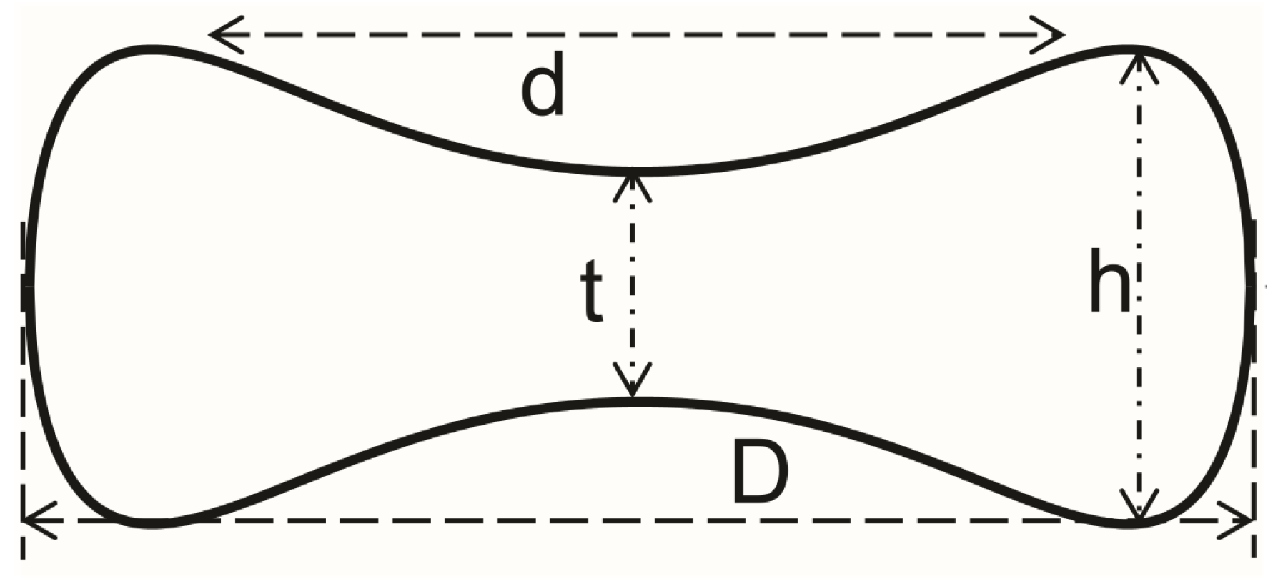
Figure 2.
Shematic diagram of the computational domain for implementing the Lippmann-Schwinger scattering series with spatially adaptive preconditioner algorithm. The black region denotes the ABL whereas the yellow region indicates the source. The computational domain consistis of a grid.
Figure 2.
Shematic diagram of the computational domain for implementing the Lippmann-Schwinger scattering series with spatially adaptive preconditioner algorithm. The black region denotes the ABL whereas the yellow region indicates the source. The computational domain consistis of a grid.
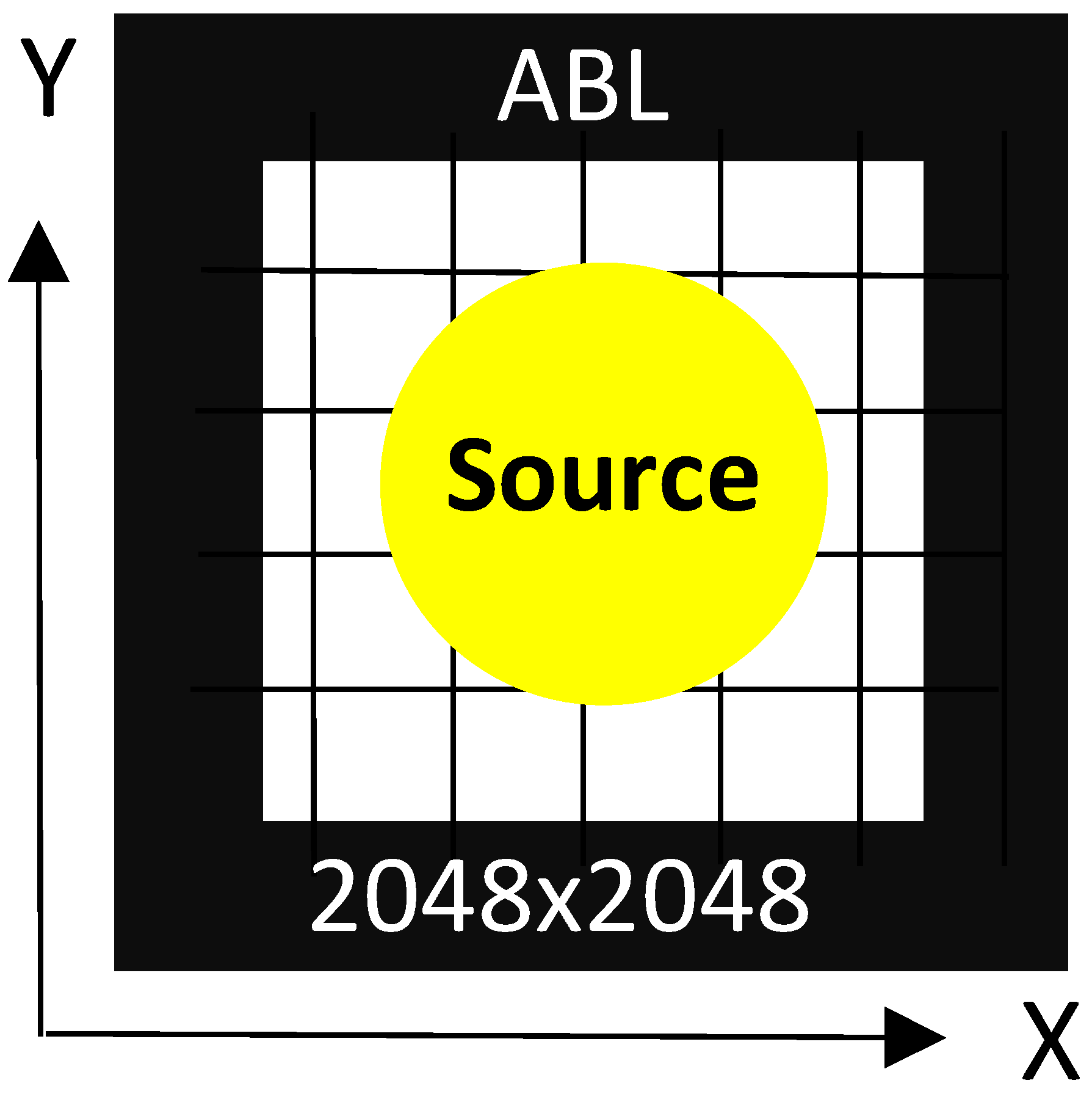
All simulations are performed within a square computational domain of size . An ABL of 100 grid points is applied arround the domain to minimize wave wrapping effects. The spatial resolution is set to nm. To further reduce artificial reflections, an exponentially decaying attenuation function is applied within the ABL region, where the parameter controls the decay near the boundaries.
For the circular disc, two different radii ( and ) are considered, and the pressure field as well as energy density () are studied under the different contrast conditions. A similar analysis is carried out for the RBC geometry and its does not depend on radii. In all cases, the density inside and outside the scatterer is assumed to be identical ( kg/). The background fluid sound speed is taken as m/s.
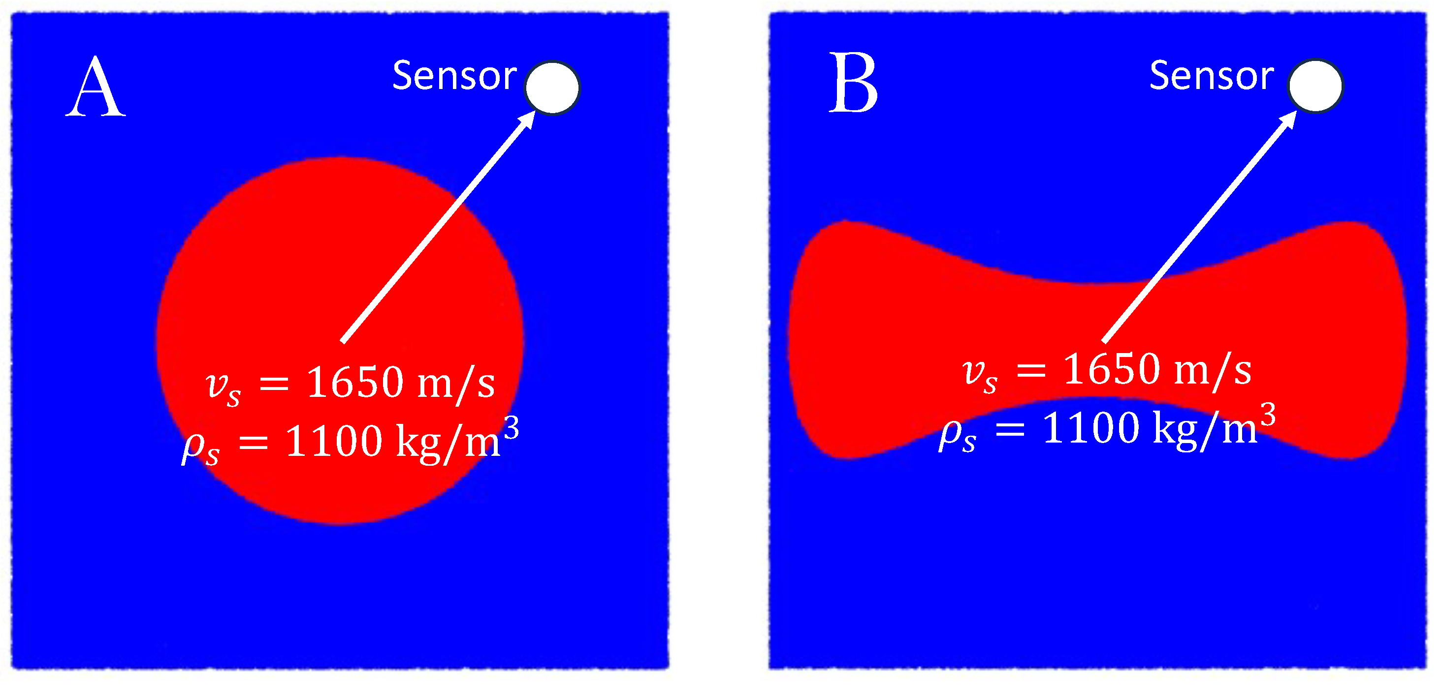
To investigate strong scattering effects, the sound speed inside the scatterer is varied, and two contrast values are considered: m/s and m/s. These choices allow us to examine the robustness of the numerical solver under high contrast conditions. All opto-thermo-mechanical parameters are assumed to be unity for simplicity. For far field and near field pressure analysis, the point sensor location is placed at a distance of from the center of the source. All numerical simulations are implemented in matrix laboratory (MATLAB). The computations are performed on a system equpped with an NVIDIA GeForce RTX 4060 GPU (302 CUDA cores, 8 GB RAM) running Ubuntu 24.04.2 LTS, using MATLAB version R2023b. MATLAB’s built in multithreading capabilities provide additional computational speed up compared to purely sequential execution.
The PA field data are collected at four different frequencies, MHz, MHz, 146 MHz and 366 MHz. Before starting the iterations, the pressure field is initialized.
Figure 3.
(a) Circular symmetry and (b) biconcave shape. A point sensor is placed at a fixed distance from the center. The blue region represents the surrounding fluid medium.
Figure 3.
(a) Circular symmetry and (b) biconcave shape. A point sensor is placed at a fixed distance from the center. The blue region represents the surrounding fluid medium.
3. Simulation Results
The Figure 4 and Figure 5 present the variation of the real part of the pressure amplitude along the x-axis. First, for the circular disc (), the pressure amplitude is shown using both RS and CBS methods along the lines , , and . In this case, the study is conducted at a frequency MHz, with the sound speed inside the source set to m/s, while the outside density and sound speed are kept constant as before. The maximum oscillation occurs at the center of the source, and the oscillation gradually decreases towards the sides.
Figure 4a along the center line, the carrier wave shows better agreement, especially at the central maxima. Moving left and right from the center line, a slight mismatch can be observed. The black dots represent the BS method, and the red line represent the CBS method. For the biconcave case, the carrier wave is also shown in Figure 5, where the real amplitude becomes slightly lower compared to the disc. Although the number of oscillations remains the same, the width of the central maxima apperas slightly narrower.
The Figure 6 and Figure 7 whow the spatial pressure distribution and energy density distribution for both the disc and RBC cases. To better visualize the distribution map, scalling has been applied up to 250 grid points on both sides along the x and y directions from the center. From Figure 6a–h, for the same radius and contrast, increasing the frequency from left to right results in an incraese in the number of rings, making the concentric circular patterns more clearly visible. As the frequency increases, the number of iterations required for convergence also increases (28, 92, 155, 310). At lower frequencies, the pressure and the energy distributions appears relatively flat and smooth, whereas at high frequencies, clear concentric circular patterns are observed. The center region defines the maximum intensity.
4. Discussion
In all cases the pressure field has a strong central maxima at the scatterer center, with oscillatory rings of decreasing amplitude outward. Both solver (RS and CBS) agree closely on the pressure profile (black dots vs. red line), indicating numerical consistency. The central focus is expected, plane wave impinging on a symmetric obstacle produces constructive interference along the symmetry axis. This pattern alligns with general scattering theory (Huygens-Fresnel).
Increasing the frequency (reducing wavelength) produces more visible interference rings and narrower main lobe. Physically, higher frequency waves resolve more of the scatterer’s geometry, leading to finer wavefront structure. In our results, the number of concentric rings grows (as shown from Figure 6a–h left to right), which is consistent with diffraction theory. Importantly, higher frequency also increases the number of iterations from 28 at the lowest frequency to over 300 at the highest. This behaviour is consistent with known properties of the CBS solver-higher contrast (higher k) slows convergence. In other words, as the effective wavenumber increases, each iteration propagates the solution over distances, requiring more itarations to reach convergence.
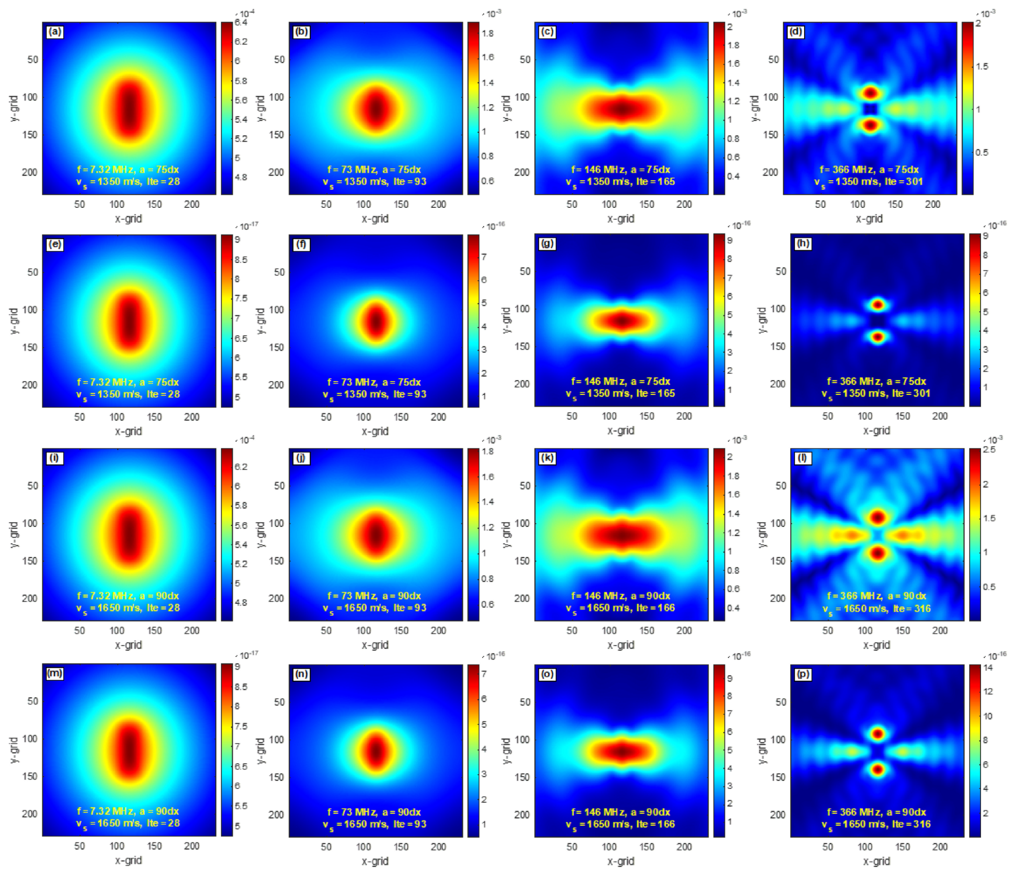
The RBC shape produces a slightly narrower central peak compared to the flat disc. Both methods yield excellent agreement in the computed fields at the center, giving confidence in the numerical implementation. The energy density distribution follows the same spatial pattern as the pressure.
5. Conclusions
The pressure field from a disk scatterer exhibits a centered high-amplitude region with concentric interference rings. These rings become more numerous and pronounced as frequency increases, reflecting the shorter wavelength; concurrently, the solver iteration count rises dramatically due to the higher effective wavenumber (consistent with Born-series convergence theory ). The RBC (biconcave) scatterer produces a qualitatively similar interference pattern, but with a modestly narrower central lobe. This confirms that the RBC’s shape influences the scattering, as predicted by prior RBC models. The two numerical methods (standard versus CBS-preconditioned) agree very well on the results, illustrating that the CBS approach is robust even under strong scattering conditions.
Acoustic intensity (energy density) maps mirror the pressure distribution, peaking at the obstacle center and forming the same ring structure, indicating conservation of energy in the scattering process. These results contribute a detailed comparison of solver methods and scatterer geometries in high-frequency acoustics. The effective validation of the CBS solver supports its use for large-scale wave problems. In practical terms, understanding how frequency and shape affect the field pattern can inform the design of ultrasonic imaging systems and targets (e.g., modeling how red blood cells interact with ultrasound).
Subsequent research could extend this framework to three-dimensional scatterers and include absorption or complex boundary conditions. For instance, modeling a suspension of RBCs or adding layered media would bring the simulation closer to biomedical scenarios. Further optimization of the solver (e.g., GPU implementation or alternative preconditioners) could improve efficiency for very high frequencies. Finally, experimental validation of these predicted patterns (especially the narrower RBC lobe) would be valuable for confirming the models.
Acknowledgments
The authors would like to thank UGC NFSC for their valuable support and financial contributions.
Conflicts of Interest
The authors declare that they have no known competing financial interests or personal relationships that could have appeared to influence the work reported in this paper.
Appendix A
Appendix A.1. Analytical Solution to the Wave Equation for Cylindrical Symmetry in Frequency Domain
Applying after appropriate boundary condition, the parametric form of Helmholtz wave equation inside and outside the cylinder,
and
Now applying the conservation equations of photoacoustics, at the point r. Both equation will satisfy at .
and
.
now,
and
Now applying the properties of Bessel’s function first kind zeroth order,
and now,
since
substitute these value into second boundary condition,
and
from A3,
From (A1) we get, the pressure field inside the cylinder,
now for outside the cylinder,
now put in (A2)
now,
The PA field at a point (inside the source) for an infinite cylinder of radius a becomes Diebold 1991,
The PA field at a point (outside the source) for an infinite cylinder of radius a becomes [7],
Here, ; J and are the Bessel function and the Hankel function of first kind, respectively. The subscripts 0 and 1 denote the orders of each function. The dimensionless quantities are defined as, and . A schematic diagram is presented in Figure 1(a). The subscript ex denotes the exact method. Equation (A5) can also be used to yield the PA field generated by a solid circle/disk if we restrict ourselves in two dimensions. Equation (A5) in the far field can be approximated as,
References
- Savéry 2007 D., Cloutier G. (2007), High-frequency ultrasound backscattering by blood: Analytical and semianalytical models of the erythrocyte cross section. The Journal of the Acoustical Society of America 122(5), 3111–3121.
- Osnabrugge 2016 G., Leedumrongwatthanakun S., Vellekoop I.M. (2016), A convergent Born series for solving the inhomogeneous Helmholtz equation in arbitrarily large media. Journal of Computational Physics 322, 113–124.
- Wang 2007 L.V., Wu H. In Biomedical Optics: Principles and Imaging; Wiley: Hoboken, NJ, 2007.
- Wang 2009 L.V. [Ed.] Photoacoustic Imaging and Spectroscopy; CRC Press: Boca Raton, FL, 2009.
- Oraevsky 1997 A.A., Esenaliev R.O., Jacques S.L., Tittel F.K. (1997), Laser-based optoacoustic imaging in biological tissues. Proceedings of SPIE 2979, 22–31.
- Wang 2016 L.V., Yao J. (2016), A practical guide to photoacoustic tomography in the life sciences. Nature Methods 13(8), 627–638.
- Diebold 1991 G.J., Sun T., Khan M.I. (1991), Photoacoustic monopole radiation in one, two, and three dimensions. Physical Review Letters 67(24), 3384–3387.
- Evans 1972 E., Fung Y.C. (1972), Improved measurements of the erythrocyte geometry. Microvascular Research 4(4), 335–347.
- Morse 1953 P.M., Feshbach H. (1953), Methods of Theoretical Physics; McGraw-Hill: New York; pp. 791–895.
- Lippmann 1950 B.A., Schwinger J. (1950), Variational principles for scattering processes. I. Physical Review 79(3), 469–480.
- Beylkin 2009 G., Kurcz C., Monzón L. (2009), Fast convolution with the free space Helmholtz Green’s function. Journal of Computational Physics 228(8), 2770–2791.
Figure 4.
The real part of the PA pressure field along the x-axis is evaluated using both the RS and CBS method at MHz for circular disc of radius , density, kg/, and sound speed, m/s. (a)-(c) Carrier wave fields measured along the grid lines at , , and , respectively.
Figure 4.
The real part of the PA pressure field along the x-axis is evaluated using both the RS and CBS method at MHz for circular disc of radius , density, kg/, and sound speed, m/s. (a)-(c) Carrier wave fields measured along the grid lines at , , and , respectively.
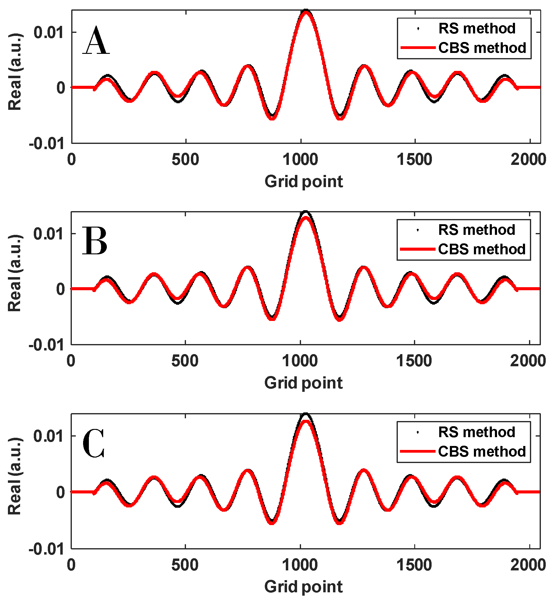
Figure 5.
Same as Figure 4 for biconcave shape but analytical (GF) and CBS methods.
Figure 5.
Same as Figure 4 for biconcave shape but analytical (GF) and CBS methods.
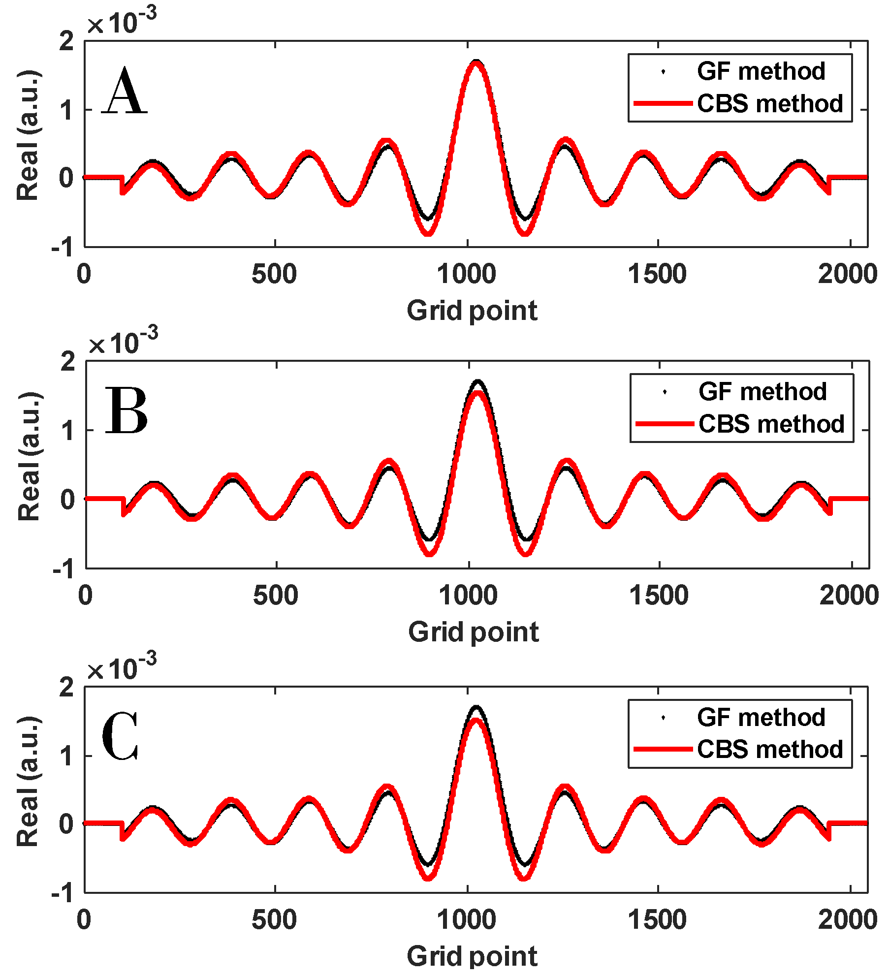
Figure 6.
Pressure and energy density distribution are computed at a distance of 250 grid points from the center along both x and y directions. (a)-(h) show results for a circular scatterer with radius and m/s, with frequency increasing from left to right ( MHz). (i)-(p) present the corresponding results for and m/s.
Figure 6.
Pressure and energy density distribution are computed at a distance of 250 grid points from the center along both x and y directions. (a)-(h) show results for a circular scatterer with radius and m/s, with frequency increasing from left to right ( MHz). (i)-(p) present the corresponding results for and m/s.
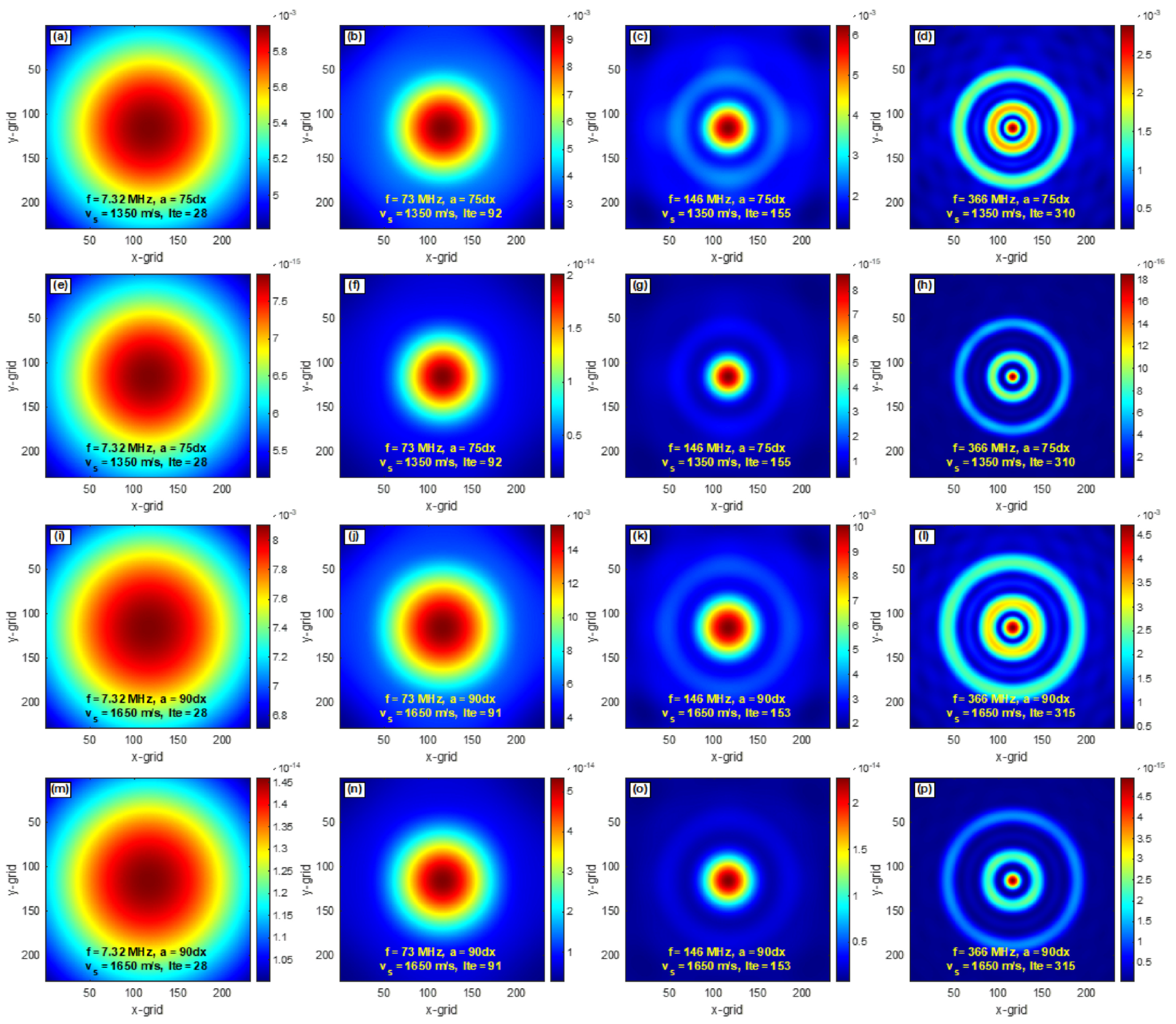
Figure 7.
Same as Figure 6 for RBC.
Figure 7.
Same as Figure 6 for RBC.
Disclaimer/Publisher’s Note: The statements, opinions and data contained in all publications are solely those of the individual author(s) and contributor(s) and not of MDPI and/or the editor(s). MDPI and/or the editor(s) disclaim responsibility for any injury to people or property resulting from any ideas, methods, instructions or products referred to in the content. |
© 2026 by the authors. Licensee MDPI, Basel, Switzerland. This article is an open access article distributed under the terms and conditions of the Creative Commons Attribution (CC BY) license (http://creativecommons.org/licenses/by/4.0/).
Copyright: This open access article is published under a Creative Commons CC BY 4.0 license, which permit the free download, distribution, and reuse, provided that the author and preprint are cited in any reuse.


