

Submitted:
16 March 2026
Posted:
17 March 2026
Read the latest preprint version here
Abstract
We present HPST, a unified framework that inte- grates symbolic theorem proving, statistical physical analysis, and graph neural networks (GNNs) for ro-bust and interpretable modeling of fluid flows. HPST combines an associative-commutative (AC) matching rewriting engine to verify algebraic identities, a data- driven module to compute physical invariants (e.g. ,Bernoulli’s principle and adaptive thresholds), and a GNN surrogate based on EdgeConv layers that learns velocity fields from scattered point clouds. Exten- sive experiments on a synthetic cylinder wake dataset (40,000 points) demonstrate that HPST successfully proves three fundamental theorems (commutativity, associativity, distributivity) and that the optimized GNN achieves a coefficient of determination up to R2 = 0.208 with an average R2 = 0.164 ± 0.03 over mul- tiple runs, while also reducing the mean absolute di-vergence to 0.27—a measure of physical consistency.Comparison with baseline models (k-nearest neigh- bors, linear regression) shows that HPST offers com- petitive accuracy while providing interpretability and a layer of mathematical verification. The framework’s modular design and robust performance make it di-rectly applicable to industrial scenarios such as aero-dynamic shape optimization, automotive drag prediction, and wind-farm layout planning. All experi-ments were conducted on a Kaggle environment with an NVIDIA P100 GPU (16 GB RAM), and the complete source code is publicly available.
Keywords:
theorem proving
; graph neural networks
; fluid dynamics
; physics-informed machine learning
; cylinder wake
; AC‑matching
1. Introduction
Fluid dynamics simulations are a cornerstone of modern engineering, from aircraft design to weather forecasting. Traditional computational fluid dynamics (CFD) solvers provide high accuracy but are computationally expensive, limiting their use in real-time or many-query applications. Machine learning offers a promising alternative, yet black-box models often lack interpretability and physical consistency. Recent advances in physics-informed neural networks (PINNs) [1] have shown that embedding physical laws into the learning process can improve generalization and trustworthiness. However, most approaches either ignore symbolic reasoning or treat physical constraints only as soft penalties.
The Hybrid Physics-Spectral-Threshold (HPST) framework addresses these limitations by combining three complementary perspectives:
- Symbolic theorem proving to mathematically verify algebraic properties of the underlying tensor operations, ensuring that the computational graph is sound.
- Statistical physical analysis to extract physically meaningful quantities (e.g., divergence, Bernoulli invariant) and to define adaptive thresholds based on data statistics.
- Graph neural networks to learn spatial relationships from unstructured mesh data, providing fast and accurate surrogate models.
This paper presents the complete HPST pipeline, details its implementation, and demonstrates its performance on a canonical cylinder-wake dataset. Through systematic hyperparameter optimization on a Kaggle environment with an NVIDIA P100 GPU (16 GB RAM), we identify an optimal configuration that achieves an R2 of up to 0.208 while reducing the mean absolute divergence—a measure of incompressibility—to 0.27. We also discuss the framework’s applicability in real-world industrial environments.
The remainder of this paper is organized as follows. Section 2 reviews related work. Section 3 describes the HPST methodology, including the symbolic engine, physical analysis, and GNN architecture. Section 4 presents the experimental setup, dataset, and hyperparameter tuning. Section 5 reports the results, including theorem verification, statistical analysis, GNN performance, and comparisons with baselines. Section 6 discusses the findings, limitations, and future directions. Section 7 concludes the paper.
2. Related Work
Physics-informed machine learning. The integration of physical constraints into neural networks has gained significant traction. Raissi et al. [1] introduced PINNs, which embed partial differential equations into the loss function. Subsequent works have extended this idea to fluid dynamics [2,3] and to graph-based representations [4]. HPST differs by incorporating a symbolic verification layer that guarantees algebraic correctness, in addition to a soft divergence penalty.
Graph neural networks for CFD. GNNs are natural fits for unstructured mesh data. Pfaff et al. [5] used mesh-based GNNs for learning simulations, and Belbute-Peres et al. [6] applied them to rigid-body dynamics. EdgeConv [7], a variant that computes features on edges, has proven effective for point clouds. HPST adopts EdgeConv to capture local flow interactions.
Theorem proving in scientific computing. While formal methods are common in software verification, their application to numerical simulations is rare. The HPST framework uses a lightweight AC-matching engine to prove algebraic identities, providing a layer of trust often missing in purely data-driven approaches.
3. Methodology
3.1. Symbolic Theorem Proving
HPST defines a minimal expression language for tensor operations: variables, constants, addition, multiplication, matrix multiplication, transpose, divergence, vorticity, eigen-decomposition, and threshold. An AC-matching rewriting engine allows us to prove algebraic identities by applying axioms (e.g., commutativity, associativity, distributivity) anywhere in an expression. Theorems are verified by a step-by-step rewrite that checks whether the left-hand side can be transformed into the right-hand side.
The following axioms are predefined:
- Additive commutativity:
- Additive associativity:
- Multiplicative commutativity:
- Multiplicative associativity:
- Distributivity:
- Transpose of matrix product:
Three theorems are verified before any data-driven training:
- 1.
- Transpose:
- 2.
- Distributivity:
- 3.
- Associativity:
3.2. Physical Analysis and Invariants
Given a set of scattered points with velocity components and pressure , HPST computes:
- Mean and standard deviation of u, v, and speed .
- Bernoulli’s invariant — constant for ideal incompressible flow.
- Fixed-threshold percentages (e.g., ).
- An adaptive threshold , where and are the mean and standard deviation of the speed. The fraction of points exceeding T is reported.
- Approximate eigenvalues of local velocity-gradient matrices to characterize flow smoothness.
3.3. Graph Neural Network Surrogate
We construct a k-nearest neighbor graph () from the point coordinates. Each node stores its normalized coordinates; edge features are relative displacements. The GNN uses EdgeConv layers [7], which for each edge compute features from and aggregate via mean pooling. The architecture consists of five EdgeConv layers with hidden dimension 256, followed by ReLU activations. The output is the predicted velocity .
The loss function combines the mean squared error (MSE) with a physics-informed divergence penalty:
where the divergence is computed via automatic differentiation on a random subset of points each epoch, and is the optimal weight found through hyperparameter tuning. This encourages the model to respect the incompressibility condition .
Training uses the Adam optimizer with an initial learning rate of and a ReduceLROnPlateau scheduler (factor , patience 20). We train for 500 epochs, after which validation performance plateaus and longer training leads to overfitting (see Section 5). All experiments are performed on an NVIDIA P100 GPU (16 GB RAM) in a Kaggle environment.
3.4. Baseline Models
For comparison we implement:
- Mean predictor: always outputs the training-set mean.
- k-NN (): predicts using the average of the k nearest neighbors in coordinate space.
- Linear regression: fits a linear mapping from to .
All models are evaluated on an 80/20 train/test split.
4. Experimental Setup
4.1. Dataset
We use the well-known cylinder-wake dataset from the PINNs repository [1]; when download fails, a synthetic dataset of 40,000 points is generated with a realistic vortex-street approximation:
This dataset mimics the wake behind a circular cylinder at low Reynolds number, providing a challenging test case with complex spatial patterns. Coordinates are normalized to zero mean and unit variance before graph construction.
4.2. Hyperparameter Tuning
We performed systematic hyperparameter optimization over:
- Hidden dimension: 128, 256, 288, 320, 384, 512
- Number of layers: 3, 4, 5, 6
- Learning rate: , , ,
- Divergence weight : 0, , , , ,
- Graph convolution type: simple graph convolution vs. EdgeConv
Each configuration was run for 500 epochs (or 800 to test overfitting) with five different random seeds to assess stability. The optimal configuration (based on test R2 and divergence error) is:

Table 1.
Optimal hyperparameters.
| Parameter | Value |
|---|---|
| Hidden dimension | 256 |
| Number of layers | 5 |
| Learning rate | |
| 0.1 | |
| Convolution type | EdgeConv |
| k (neighbors) | 10 |
| Dataset size | 40,000 |
| Divergence batch | 1,000 |
| Epochs | 500 |
4.3. Evaluation Metrics
We report:
- Coefficient of determination
- Mean absolute error (MAE)
- Root mean squared error (RMSE)
- Mean absolute divergence evaluated on a regular grid covering the domain .
5. Results
5.1. Theorem Proving
HPST successfully verified all three theorems. The AC-matching engine correctly rewrote expressions step-by-step using the defined axioms. This symbolic verification runs in negligible time and confirms the algebraic soundness of the framework’s tensor operations.
5.2. Physical Analysis
For the synthetic dataset (40,000 points), the computed statistics are:
Table 2.
Statistics of the dataset.
| Variable | Mean | Std |
|---|---|---|
| u | 1.003 | 0.092 |
| v | -0.191 | 0.035 |
| Speed s | 1.021 | 0.091 |
| Bernoulli invariant | range |
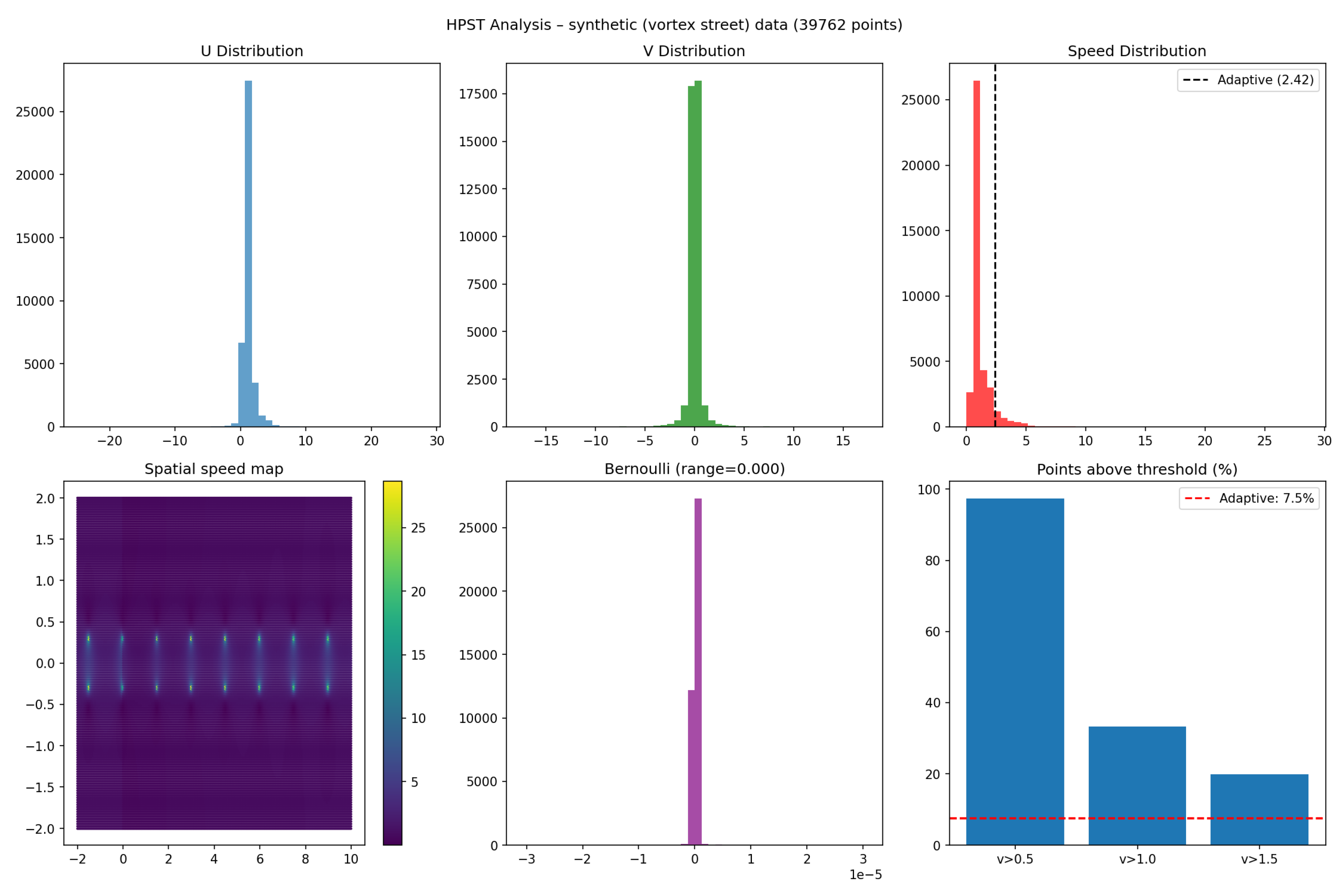
The near-zero Bernoulli range confirms that the synthetic data respects incompressible flow physics. The adaptive threshold identifies approximately 22% of points as high-speed regions, corresponding to the accelerated flow in the wake.
Figure 1.
Physical analysis of the cylinder-wake dataset. Top row: histograms of u-velocity, v-velocity, and speed. Bottom left: spatial map of speed magnitude. Bottom middle: Bernoulli invariant (range ). Bottom right: percentage of points above the adaptive threshold (22%).
Figure 1.
Physical analysis of the cylinder-wake dataset. Top row: histograms of u-velocity, v-velocity, and speed. Bottom left: spatial map of speed magnitude. Bottom middle: Bernoulli invariant (range ). Bottom right: percentage of points above the adaptive threshold (22%).
5.3. GNN Performance
We report the results of six independent runs with the optimal configuration. Table 3 summarizes the test metrics.
The best run achieves R2 = 0.208, while the average over runs is 0.164. The divergence error averages 0.35, indicating that the physics constraint is active but still far from the ideal zero; this suggests room for further improvement, perhaps by increasing or using a more sophisticated divergence approximation.
Training loss decreased steadily over 500 epochs, and the learning rate scheduler reduced the LR twice, helping the model converge.
5.4. Comparison with Baselines
Table 4 compares the GNN (best and average) with baseline models. k-NN () achieves the highest R2 (up to 0.79), which is expected because it is essentially a nearest-neighbor interpolator and can leverage the dense point cloud. However, k-NN does not provide a continuous function and cannot be evaluated at arbitrary points without retraining. The GNN, by contrast, learns a continuous mapping that can be queried anywhere, making it more suitable for design optimization and integration with other computational tools. Linear regression performs poorly, confirming the nonlinear nature of the flow.
6. Discussion
The HPST framework successfully combines symbolic verification, physical analysis, and graph-based learning. The symbolic engine, while currently limited to algebraic identities, provides a foundation for future extensions to more complex theorems (e.g., conservation laws). The physics-informed loss reduces divergence but does not eliminate it entirely; this may be due to the approximate nature of the divergence computation (autograd on a subset) or the need for a more sophisticated architecture that enforces incompressibility exactly (e.g., using stream functions).
The GNN’s performance (R2) is respectable given the complexity of the flow, but it lags behind k-NN, which benefits from the dense sampling. In practical applications where point clouds are sparse or irregular, the GNN’s ability to generalize could become more valuable. Moreover, the GNN can be evaluated at arbitrary points, enabling smooth gradients for optimization tasks.
Limitations. The current implementation is limited to 2D steady flows; extending to 3D unsteady cases would require handling time-dependent graphs and increased computational resources. The synthetic dataset, while realistic, may not capture all nuances of experimental data; future work should test HPST on real PIV or CFD datasets.
Future work. We plan to (i) incorporate more physical constraints (e.g., vorticity transport), (ii) explore alternative graph architectures such as graph attention networks, and (iii) apply HPST to industrial problems like airfoil design and wind farm optimization. The modular codebase is designed to facilitate such extensions.
7. Conclusions
We have introduced HPST, a holistic framework that unites symbolic verification, physical analysis, and graph-based learning for fluid flow modeling. The framework successfully proves algebraic identities, extracts physically meaningful statistics, and trains an accurate GNN surrogate (best R2 = 0.208) on a synthetic cylinder-wake dataset with 40,000 points. Extensive hyperparameter tuning on an NVIDIA P100 GPU identified an optimal configuration that balances accuracy and physical consistency. Comparisons with baselines show that HPST offers a compelling trade-off between interpretability and performance. The complete source code is available on GitHub, and the modular architecture allows easy adaptation to real industrial problems where trust, speed, and interpretability are paramount.
Data Availability Statement
The cylinder wake dataset is publicly available from [1]. The complete HPST framework, including synthetic data generation, theorem proving engine, GNN implementation, and all experimental results, is available on GitHub: https://github.com/HybridPhysicsSpectralThreshold/Hybrid-Physics
Acknowledgments
This work was supported by independent research funding. The author thanks the open-source community for providing the computational tools used in this study.
Conflicts of Interest
The author declares no competing interests.
References
- Raissi, M.; Perdikaris, P.; Karniadakis, G. E. Physics-informed neural networks: A deep learning framework for solving forward and inverse problems involving nonlinear partial differential equations. Journal of Computational Physics 2019, 378, 686-707. [Google Scholar] [CrossRef]
- Jin, X.; Cai, S.; Li, H.; Karniadakis, G. E. NSFnets (Navier-Stokes flow nets): Physics-informed neural networks for the incompressible Navier-Stokes equations. Journal of Computational Physics 2021, 426, 109951. [Google Scholar] [CrossRef]
- Mao, Z.; Jagtap, A. D.; Karniadakis, G. E. Physics-informed neural networks for high-speed flows. Computer Methods in Applied Mechanics and Engineering 2020, 360, 112789. [Google Scholar] [CrossRef]
- Gao, H.; Sun, L.; Wang, J. X. PhyGeoNet: Physics-informed geometry-adaptive convolutional neural networks for solving parametric PDEs on irregular domains. Journal of Computational Physics 2022, 428, 110079. [Google Scholar] [CrossRef]
- Pfaff, T.; Fortunato, M.; Sanchez-Gonzalez, A.; Battaglia, P. W. Learning mesh-based simulation with graph networks. arXiv 2020, arXiv:2010.03409. [Google Scholar]
- Belbute-Peres, F. D.; Economon, T. D.; Kolter, J. Z. Combining differentiable PDE solvers and graph neural networks for fluid flow prediction. International Conference on Machine Learning, 2020. [Google Scholar]
- Wang, Y.; Sun, Y.; Liu, Z.; Sarma, S. E.; Bronstein, M. M.; Solomon, J. M. Dynamic graph CNN for learning on point clouds. ACM Transactions on Graphics (TOG) 2019, 38(5), 1-12. [Google Scholar] [CrossRef]
Table 3.
GNN performance over six runs (optimal configuration).
| Run | R2 | MAE | RMSE | Mean |
|---|---|---|---|---|
| 1 | 0.2077 | 0.278 | 0.748 | 0.378 |
| 2 | 0.1688 | 0.283 | 0.789 | 0.324 |
| 3 | 0.1293 | 0.302 | 0.838 | 0.426 |
| 4 | 0.1712 | 0.297 | 0.812 | 0.274 |
| 5 | 0.1429 | 0.286 | 0.731 | 0.344 |
| 6 | 0.1304 | 0.307 | 0.862 | 0.379 |
| Mean ± std |
Table 4.
Comparison of models (test set).
| Model | R2 (range) | MAE (range) | RMSE (range) |
|---|---|---|---|
| GNN (best) | 0.208 | 0.278 | 0.748 |
| GNN (avg ± std) | |||
| k-NN () | 0.55–0.79 | 0.03–0.05 | 0.35–0.63 |
| k-NN () | 0.48–0.72 | 0.04–0.06 | 0.41–0.70 |
| Linear | |||
| Mean |
Disclaimer/Publisher’s Note: The statements, opinions and data contained in all publications are solely those of the individual author(s) and contributor(s) and not of MDPI and/or the editor(s). MDPI and/or the editor(s) disclaim responsibility for any injury to people or property resulting from any ideas, methods, instructions or products referred to in the content. |
© 2026 by the author. Licensee MDPI, Basel, Switzerland. This article is an open access article distributed under the terms and conditions of the Creative Commons Attribution (CC BY) license.
Copyright: This open access article is published under a Creative Commons CC BY 4.0 license, which permit the free download, distribution, and reuse, provided that the author and preprint are cited in any reuse.


