

Submitted:
07 March 2026
Posted:
10 March 2026
You are already at the latest version
Abstract
Hyperspectral imaging integrates spatial and spectral data, crucial for environmental and vision science applications. Existing spectroradiometers lack spatial resolution, and many hyperspectral systems are costly or unsuitable for fieldwork mimicking human vision. Here, we present the development of a portable, relatively low-cost hyperspectral camera based on a tunable filter and a commercial video camera, together with Python-based software capable of generating hyperspectral cubes from the acquired images, as a more accessible and adaptable alternative for specific applications.
The proposed method includes assembling the acquisition system and processing raw images, which have been demosaiced, linearized, and labeled with their corresponding spectral band, to generate a hyperspectral cube. Our approach allows radiance retrieval through prior calibration or reflectance estimation using a white reference from a selected region of the hyperspectral cube. Additionally, it enables exporting the hyperspectral cube as a three-dimensional matrix. The developed software facilitates visualization and analysis of hyperspectral data.
Validation against a spectroradiometer demonstrated reliable spectral radiance measurements under moderate to high light conditions. This adaptable approach enhances accessibility to hyperspectral imaging for research contexts with limited resources, supporting detailed visual environment characterization outside controlled laboratory settings.
Keywords:
field spectral measurements
; hypercube
; hyperspectral imaging
; imaging system
; short-range
1. Introduction
Hyperspectral imaging (HSI) has emerged as a key tool for the simultaneous capture of spectral and spatial information, integrating both dimensions into a single dataset. This technology makes it possible to obtain, for each pixel in an image, spectral measurements across multiple wavelengths, enabling detailed analysis of the radiometric properties of the materials present in a scene. Owing to these capabilities, HSI is widely used in diverse scientific and technological fields, such as remote sensing [1,2], industrial inspection [3], biomedical imaging [4,5], and vision science [6,7], among others. Traditionally, spectral information has been acquired using conventional spectroradiometers, which provide precise spectral measurements but lack spatial resolution because they integrate the signal from a given area within the field of view [8]. This characteristic limits their application in the characterization of extended, heterogeneous, or dynamic scenes. In response to this limitation, HSI systems were developed to simultaneously record the spatial and spectral variability of a scene, generating matrix datasets typically organized into hyperspectral cubes composed of two spatial dimensions and one spectral dimension [9], with acquisition times ranging from milliseconds to seconds, or even enabling instantaneous capture, depending on the technology employed [1,2]. Methods for HSI acquisition have progressively evolved alongside technological advances. Early systems employed configurations based on moving mirrors and point spectroradiometers, or on linear sensor arrays, enabling reconstruction of the hyperspectral cube through spatial scanning [9]. These approaches were later optimized and became widely used in remote sensing applications, both on satellite platforms [10] and in airborne systems, including those mounted on drones [11]. With the miniaturization of technology, more compact developments emerged, such as the so-called HOSI camera [12], which uses a mobile spectroradiometer to acquire spatial information from a scene, as well as systems designed for retinal imaging [4]. In parallel, advances in high-sensitivity, high-speed CMOS sensors enabled alternative hyperspectral capture methods, such as the use of tunable filters [13] or CMOS sensors with broadband filter patterns, from which the spectral dimension is reconstructed through computational processing [14]. In this context, although the aforementioned developments represent significant contributions to spectral data acquisition—especially for remote or distance-capture applications—some systems rely on device or platform motion and therefore lack sufficient stability to obtain hyperspectral cubes suitable for visual environment characterization in fieldwork conditions [15], while others may not offer adequate spectral or spatial resolution to study the visual environment from an anthropocentric perspective [1,16]. Moreover, although hyperspectral systems designed for industrial applications exhibit a high degree of technological maturity [3], these cameras are often expensive, fragile, and not always suitable for research outside controlled environments [17]. Taken together, these limitations reduce their suitability for field campaigns, where conditions often involve limited control over device motion, scene dynamics, and power supply, thereby compromising the acquisition of reliable HSI data. Furthermore, previous HSI devices may not fully exploit recent advances in commercial RGB cameras to approximate natural vision [18,19,20]. To address these challenges, we developed an portable, adaptable HSI system based on a commercial camera coupled with a tunable filter, capable of obtaining spectral information with high spatial resolution while remaining relatively low-cost, robust, and suitable for fieldwork. The proposed system takes advantage of the commercial camera’s ability to record uncompressed image sequences, synchronizing them with a programmable filter to generate hyperspectral cubes in the visible range that are well-suited for studies focused on human visual perception. The aim of this article is to present both the hardware and software components of the developed system and demonstrate its potential for performing hyperspectral measurements in diverse environments outside the laboratory. Compared with commercial solutions, our approach offers enhanced flexibility, adaptability, and cost-efficiency for field-based visual environment characterization.
2. Materials and Methods
2.1. The Hardware
To obtain spatially resolved spectral information from real-world environments (i.e., uncontrolled settings), we used a video camera with red, green and blue sensors (RGB), a tunable wavelength filter operating from 420 nm to 720 nm, and a lens system. In addition, this work includes the development and implementation of a Python-based software pipeline capable of: (i) controlling the tunable filter through the library provided by the filter manufacturer (Thorlabs), which initializes the device and sets the desired wavelength; (ii) using the Sounddevice library to emit an audio signal that links the wavelength configured in the tunable filter with the image captured by the camera via a Windows-based computer interface; and (iii) managing raw image processing (demosaicing, linearization, and spectral band labeling) and generating hyperspectral cubes in HDF5 (.H5) format. This software also enables the calculation of radiance and reflectance using previously obtained calibration data or white reference measurements.
2.1.1. The RGB Video Camera
To select the acquisition system, the main criteria considered were sensitivity, dynamic range, and image acquisition speed. In an initial stage, a comparative evaluation was conducted on four different cameras: two DSLR models (Canon 5D Mk II and Canon T3i), one scientific-grade camera (QImaging QICAM FAST 1394), and a Blackmagic Cinema Camera 2.5K [21], in order to determine the most suitable device for the proposed system. All cameras met the sensitivity requirement, demonstrating adequate performance under low-illumination conditions [22]. However, although the Canon cameras exhibited good dynamic range, they exhibited relatively slow inter-frame acquisition times [23,24]. In the case of the QImaging camera, acquisition speed depended on software configuration; nevertheless, this device was discarded due to its connection interface (FireWire 1394), considered obsolete. For these reasons, the camera ultimately selected for constructing the hyperspectral imaging system was the Blackmagic Cinema Camera (BMCC).
The BMCC can record between 24 and 30 images per second with a 12-bit depth and provide a wide dynamic range [21]. It also offers the possibility of saving image sequences in raw (.DNG) format together with a separate audio file directly to a solid-state drive (SSD), without requiring an external computer. Image capture is performed without spatial or temporal compression, ensuring a high degree of control and fidelity in the acquired data [21].
The raw files generated by the camera can be processed using open-source libraries such as Rawpy [25], allowing near-complete control over the digital development pipeline. However, in this work the raw files were used without post-processing, and demosaicing was performed manually, without pixel interpolation. In this way, it is possible to obtain information from the three primary sensor channels independently, as shown in Figure 1.
Although the native sensor resolution is 2432 × 1366 pixels, because it uses a Bayer pattern, each channel is subsampled, with an effective resolution of approximately 608 × 341 pixels per channel.
2.1.2. The Tunable Wavelength Filter
For the spectral filtering of light, we used a KURIOS-XL1/M tunable filter [26] to selectively transmit narrow wavelength bands within the 420 nm to 720 nm range before reaching the camera sensor, with transmittance varying from 1% at shorter wavelengths to 43% at longer wavelengths (Figure 2).
This tunable filter can be controlled using its Software Development Kit (SDK) libraries. These libraries enable programmable control of the filter through programming languages such as C++, LabVIEW, and Python, providing flexibility for integration into different projects. Python was selected as the programming language because it can be used on portable devices such as laptops and tablets.
2.1.3. Integration of the Camera with the Tunable Filter
To integrate the tunable filter with the camera, several mechanical adaptations were required, including 3D-printed components as well as the incorporation of an intermediate optical system. The camera features a Canon EF mount with a flange distance of 44 mm, whereas the tunable filter has a thickness of 60.5 mm. Due to the mismatch in flange distance and mechanical dimensions, a lens was inserted between the camera mount and the tunable filter, and an additional lens was placed between the tunable filter and the primary lens, as shown in Figure 3. This configuration preserves compatibility with interchangeable commercial Canon lenses and makes it possible to vary the field of view and, consequently, the data acquisition area without modifying the rest of the experimental setup.
2.2. Acquisition and Synchronization Protocol
During acquisition, the BMCC generates a sequence of 24 frames, with an approximate size of 3 MB per frame [21]. These frame files are automatically stored in a folder together with the corresponding audio file. This folder is created with a name composed of the camera model, date, hour, minute, and a clip identifier. Each image in the sequence is saved with a similar filename to which a consecutive frame number is added, allowing each image to be associated with a specific time instant from the beginning of the recording.
Similarly, the audio file contains an accurate temporal reference, since the sampling frequency remains constant throughout the entire capture. This temporal correspondence between the frame sequence and the audio signal makes it possible to relate each frame to a defined acquisition instant and, therefore, to the specific spectral range associated with that frame during the spectral sweep of the tunable filter.
The complete acquisition and processing workflow, from the scene to hyperspectral cube generation, is summarized in Figure 4. Light from the scene enters through the lens, passes through the tunable filter (Kurios XL1/M), and is recorded by the camera (Blackmagic Cinema Camera 2.5K) sensor through sequential acquisition at different spectral bands. The spectral variation of the filter is controlled by a software-generated signal (Synchronization module), which simultaneously sends an audio signal that is recorded together with the image sequence captured by the camera. In this way, each frame becomes temporally associated with a specific portion of the audio signal, enabling precise correspondence between acquisition time and the spectral range transmitted by the filter. If a reference white, such as Polytetrafluoroethylene (PTFE) sample or another calibrated white target, is included, spectral reflectance can be obtained using this information. Subsequently, the images are processed and computationally reorganized to reconstruct the hyperspectral cube while preserving the spatial and spectral dimensions of the scene.
2.3. The software
The developed software is organized into three main modules: (i) control of the tunable filter and synchronization of each spectral band with the images acquired by the camera; (ii) construction of the hyperspectral cube; and (iii) visualization of the hyperspectral cube and extraction of associated data.
The software was developed in Python, and the required libraries can be installed using the pip package manager, except for the libraries specific to the tunable filter, which can be downloaded from the manufacturer’s website [26].
The first module of the software is an independent script that controls the tunable filter and sends synchronization information to the camera. The software initializes the tunable filter by setting it to its minimum transmission (black) state, ensuring that acquisition always begins from the same spectral condition. The system is then sequentially configured, starting at 420 nm and increasing the central wavelength in 10 nm steps until reaching 720 nm. In parallel, an audio signal is emitted and recorded by the camera, as shown in Figure 5.
The second module provides three main options: Create Hypercube, Open Hypercube, and Camera Spectral Calibration. The Create Hypercube option generates the hyperspectral cube from the files captured by the camera. To do so, the program requests the associated audio file, located in the same folder as the raw image sequence. A series of dialog boxes is then displayed for the user to define the parameters required for the hyperspectral cube construction.
Once the hyperspectral cube has been generated and loaded, the Open Hypercube option provides access to an interface designed for interactive visualization and data analysis. In this interface, the cube is initially displayed as an RGB image composed of three selected spectral bands at 650 nm, 550 nm, and 450 nm, assigned to the red, green, and blue channels, respectively. In the viewer, a red rectangle indicates the region of interest used for spatial integration and spectral computation.
Below the main viewer, the average spectral radiance curve corresponding to the selected area is displayed, along with descriptive statistics including the mean value, standard deviation, and minimum and maximum pixel values within the selected region. Additionally, to the right of the image, a wavelength-encoded vectorscope is shown, allowing visualization of the spectral distribution of pixel density within the selected section (Figure 6). The system also enables calculation of both radiance and reflectance, provided that a PTFE reference is available.
For reflectance measurements, the software allows loading PTFE reference data obtained from an image and reusing it for calibrating subsequent acquisitions. This functionality is particularly useful when multiple images are acquired within the same session and under similar illumination conditions, since it enables reflectance estimation without physically including the PTFE reference in every scene, thereby facilitating data acquisition in natural or hard-to-access environments.
2.4. Characterization and Calibration
2.4.1. Dynamic Range and Linearization
Dynamic range was measured using an X-Rite color chart illuminated with cool white light-emitting diode (LED) lamps inside a diffuse light booth (Figure 7) [27]. To establish the reference luminance values of the color chart, the range of luminances present in natural environments was considered. For this purpose, luminance measurements were taken in a natural outdoor environment at midday (13:00 h) during spring, recording values corresponding to overcast sky away from the solar disk (11,000–20,000 cd/m²), clear sky (11,000–16,000 cd/m²), concrete surfaces under direct sunlight (9,000–11,000 cd/m²), and ground under the shade of a small forest (200–400 cd/m²).
Subsequently, in the laboratory, the color chart was illuminated until reaching a 29,000 cd/m². The highest possible sensitivity was then selected without saturating the camera sensor at the wavelength of maximum response (540 nm). Consequently, an ISO sensitivity of 1600 was used and the shutter angle was set to 180°, although the camera allows shorter exposure times. To maintain adequate exposure while avoiding sensor saturation, a 50 mm lens with an f/1.4 aperture was used.
To evaluate the radiometric linearity and dynamic range of the sensor, 29 hyperspectral cubes were acquired, each accompanied by its corresponding spectral radiance measurement taken over a PTFE reference. Throughout the entire experimental process, the positions of the spectroradiometer, hyperspectral camera, and reference chart inside the diffuse illumination booth were kept fixed in order to ensure constant geometric and observation conditions (Figure 8a).
Variation of the incident radiance was achieved through progressive control of the booth illumination, sequentially switching off the luminaires to obtain an approximately uniform decrease in illumination level down to low values, as shown in Figure 8a. For luminance levels below 10 cd/m², an additional external luminaire was used, whose distance and orientation were adjusted to reach the required minimum values.
The curve obtained after analyzing the linearization data (Figure 8b) shows a non-linear response that approximates proportionality over the analyzed range; however, the relationship is not strictly linear. For this reason, a linearization correction look up table was constructed to compensate for the sensor’s non-linearity and obtain a linear relationship between physical radiance and the measured digital signal.
From these measurements, an effective dynamic range of approximately 4.4 orders of magnitude was determined, spanning from 0.4473 W·m⁻² to 1.02 × 10⁻⁵ W·m⁻² at 540 nm. This interval defines the radiance limits within which the system maintains a stable and usable response.
It is important to distinguish between the absolute radiance range measured at 540 nm—which depends on the transmittance of the tunable filter and the optical efficiency of the system—and the sensor’s dynamic range, expressed in orders of magnitude, which characterizes the system’s ability to resolve signals between the noise threshold and the saturation level. The effective dynamic range of the system corresponds to approximately 4.38 orders of magnitude. For other wavelength groups, the dynamic range is maintained, but sensitivity depends on the spectral transmittance of the filter at each wavelength.
2.4.2. Homogenization
Commercial cameras consist of a body that houses the sensor, responsible for recording incident light, and a lens coupled through a mount designed to minimize optical aberrations. However, when the original optical system is modified by incorporating a tunable filter and an additional lens system, the way light reaches the sensor is altered, affecting the homogeneity of the response at each wavelength.
To correct this inhomogeneity, a white surface was uniformly illuminated and a reference hyperspectral image (WR) was acquired. From this image, the mean value (WM) was calculated for each wavelength. Since the ideal reference scene should exhibit spatial uniformity, a negative inhomogeneity map (Hmap) was generated by dividing WM by WR, as expressed in Equation (1).
Homogeneity correction was performed by multiplying the Hmap by a sample image. The effect of this correction is clearly visible, as shown in Figure 9. It should be noted that, because this correction is applied during post-processing, it presents limitations associated with both sensor sensitivity and the spatial distribution of illumination across the sensor.
Hmap = WM / WR
2.4.3. Calibration
The signal recorded in the raw files of the hyperspectral system is determined by the interaction between the spectral radiance of the scene, the spectral sensitivity of the sensor, and the spectral transmittance of the tunable filter. Because both sensor sensitivity and filter transmittance vary with wavelength, the system response is not uniform across the spectrum and requires wavelength-dependent correction coefficients.
The calibration procedure was carried out using a spectroradiometer as a radiometric reference. For this purpose, a diffuse PTFE surface was illuminated with a cool LED light source, and spectral measurements were acquired both with the spectroradiometer and with the hyperspectral camera. Both measurements were performed from the same position and under identical illumination conditions, ensuring that the observed spectral radiance was equivalent for both instruments.
From these measurements, a wavelength-dependent correction coefficient was calculated by directly comparing the spectral radiance measured by the spectroradiometer with the digital signal recorded by the hyperspectral camera, as shown in Equation 2, where C(λ) is the spectral correction coefficient, Lspec(λ) is the spectral radiance measured by the spectroradiometer over the PTFE surface, and Dcam(λ) is the average digital signal recorded by the hyperspectral camera at the corresponding wavelength.
C(λ) = Lspec(λ)/Dcam(λ)
This coefficient integrates into a single wavelength-dependent factor the spectral variations introduced by sensor sensitivity, the transmittance of the tunable filter, and the spectral distribution of the illuminant.
Applying these correction coefficients at each wavelength makes it possible to adjust the spectral response of the camera so that it is consistent with spectroradiometer measurements, Consequently, the calibration is valid under illumination conditions spectrally equivalent to those used during coefficient estimation. Because the coefficient is derived from an absolute radiometric reference, the calibrated camera data can be directly compared with absolute spectral measurements within the limits imposed by the uniformity of the diffuse surface and the sensitivity of the sensor.
To obtain the final calibrated signal, the raw digital signal recorded by the camera (Dcam) is corrected by sequentially applying, for each spectral band, the homogeneity map (Hmap) and the spectral calibration coefficient (C), resulting in the multiplication Dcam(λ) · Hmap(λ) · C(λ), which compensates both spatial inhomogeneities of the system and wavelength-dependent variations introduced by the sensor and the tunable filter.
3. Results
3.1. Validation
3.1.1. Radiance Profile
The experimental setup shown in Figure 7 was used to acquire hyperspectral cubes and perform radiance measurements on a PTFE surface illuminated with different levels of cool white LED, with the aim of comparing radiance measurements obtained with the hyperspectral camera and the reference spectroradiometer. Table 1 presents the comparison of spectral radiance at 540 nm for different signal levels, identified as Lin_w_XX. It includes absolute radiance values expressed in W·m⁻²·nm⁻¹, as well as the percentage difference between both systems, reported both individually and as an average across the measured spectral range.
The agreement between the hyperspectral camera and spectroradiometer measurements was evaluated as a function of the analyzed radiance range. In most cases, individual differences remained below ±2%, indicating a high level of consistency between the two systems under medium and high signal conditions. However, as the radiance level decreased until very low levels, the developed hyperspectral camera sensor exhibited reduced sensitivity, resulting in an increase in the relative difference between the devices. This effect is particularly evident at the lowest radiance levels (Lin_w_033 and Lin_w_035), where the average difference increased significantly, suggesting an increased influence of noise and relative error amplification at very low signal levels.
Overall, these results indicate that both systems exhibit consistent and comparable performance under medium and high radiance conditions, whereas the discrepancies observed at low radiance levels should be interpreted with caution, given the amplification of percentage error at very low absolute radiance values.
Additionally, Figure 10 presents a spectral comparison of the percentage deviation between measurements obtained with the hyperspectral camera and the reference spectroradiometer for each signal level (Lin_w_XX) as a function of wavelength. This spectral analysis enables a more detailed evaluation of system performance across the visible range and facilitates the identification of patterns associated with noise and sensitivity limitations.
For medium and high radiance levels (Lin_w_08 to Lin_w_030), the deviation remains close to zero across most of the spectrum. In contrast, for the lowest radiance levels (Lin_w_033 and Lin_w_035), significantly larger deviations are observed, particularly at short wavelengths (420–470 nm) and long wavelengths (640–720 nm), where the relative error greatly exceeds that of the rest of the spectrum. This behavior is consistent with lower tunable filter transmittance at short wavelengths and reduced sensitivity of the sensor’s green channel within those wavelength groups.
Overall, these analyses show that the system performs well under moderate radiance conditions, whereas measurements acquired at low signal levels require careful treatment due to noise.
3.1.2. Spectral Agreement
Although percentage deviation analysis is a useful metric for quantifying the performance of the developed hyperspectral camera, an additional test was conducted to validate its spectral reconstruction performance under realistic measurement conditions. For this purpose, spectral measurements were performed on a color chart under the same illumination conditions used during the calibration process.
The curves obtained, shown in Figure 11, exhibit consistent spectral agreement between measurements, with each chromatic patch displaying a distinct spectral signature identifiable with its corresponding color. The shapes of the curves, their relative maxima, and their slopes match the expected behavior for each patch, indicating that the system correctly preserves relative spectral information in reflectance measurements. Taken together, these results indicate that the hyperspectral camera is capable of reconstructing physically consistent spectral information within the visible range.
The spectral responses plotted in Figure 11 indicate that the system achieves maximum spectral accuracy within the mid-visible range and shows increasing deviations toward the spectral extremes, a behavior consistent with the physical limitations of the sensor’s green channel and the tunable filter’s lower transmittance at shorter wavelengths. Overall, the error distribution does not exhibit abrupt systematic biases or large spectral irregularities, supporting the validity of the calibration and the reliability of the hyperspectral camera’s spectral performance.
3.2. Performance in the Field
In terms of implementation and field use, the developed hyperspectral camera features a compact and portable design that enables operation outside the laboratory. The system can be mounted inside the trunk of a vehicle (Figure 12a) and controlled via a computer tablet (Figure 12b), facilitating configuration and remote operation. The BMCC includes an internal battery, and given the tunable filter’s low power consumption, the system can operate using the vehicle’s battery, providing greater flexibility in selecting acquisition scenarios and conditions for hyperspectral imaging.
Hyperspectral image acquisition is performed within a short time: the system requires approximately 7 seconds to capture a hyperspectral cube composed of 31 spectral bands in the visible range, from 420 nm to 720 nm, with a spectral sampling interval of 10 nm. Although the BMCC is capable of generating up to 30 frames per second [21], the switching time between bands of the tunable filter constitutes a limiting factor, thereby limiting further reduction of total acquisition time.
4. Discussion
We developed a portable hyperspectral camera based on a tunable filter coupled to a commercial CMOS camera, with the aim of enabling spectral measurements of natural scenes under real observation conditions. The hyperspectral camera was designed to operate in field campaigns where environmental control is limited and acquisition geometry is centered on human vision [7,10,15].
Comparisons with the reference spectroradiometer show that the proposed system reproduces spectral radiance in the visible range with good agreement under medium and high radiance conditions. Both the point analysis at 540 nm and the full spectral comparison indicate small relative deviations and coherent spectral behavior across most of the visible range. The discrepancies observed at low radiance levels are primarily attributed to signal-to-noise ratio limitations rather than to systematic differences in spectral response, data acquisition, or processing.
In other hyperspectral camera developments [12,17], exposure time is adjusted according to wavelength to maximize effective dynamic range per pixel. However, the commercial camera employed in our system does not allow independent exposure control for each spectral band or real-time remote parameter modification with immediate feedback [21]. Consequently, each hyperspectral cube is acquired using a single configuration of exposure, ISO sensitivity, and aperture. Despite this constraint, the system provides a sufficiently wide dynamic range to capture spectral information in both shadowed areas (e.g., under vegetation cover) and high-luminance areas such as clear skies.
The acquisition time (approximately 7 seconds per cube) is compatible with moderate environmental stability, where factors like breeze or gradual illumination changes do not introduce significant spatial distortions. This is particularly relevant in natural environments, where movement of leaves, branches, or clouds may affect spatial consistency between spectral bands. Additionally, the availability of multiple frames per spectral band (the system generates approximately five images per spectral band) opens possibilities for future software improvements, such as noise reduction strategies through temporal averaging.
The selection of the BMCC as the capture device for the proposed hyperspectral system represents a compromise between radiometric performance, processing control, and accessibility. The BMCC provides direct access to high bit-depth uncompressed raw data, enabling fully customized acquisition and processing workflows. This feature is especially relevant for experiments requiring precise control over each stage of processing. Moreover, its ability to operate autonomously—recording sequences onto an SSD without relying on an external computer—facilitates its use in fieldwork and portable experimental setups. Its mechanical robustness and second-hand market availability further make it an economically viable option for low-cost developments, allowing system replication without specialized equipment or complex laboratory infrastructure. The camera functions as a highly sensitive radiometric sensor that, combined with spectral filtering and sequential acquisition techniques, enables reconstruction of hyperspectral cubes suitable for characterizing the visual environment under real observation conditions. However, it is not the only video camera capable of meeting these requirements. While alternative cameras such as ZCAM, RED, or SONY offer comparable capabilities, proprietary raw formats may limit low-level access. Meanwhile, recent advances in mirrorless cameras, particularly in burst shooting speed and sensitivity [28,29], open new possibilities for developing hyperspectral systems based on tunable filters. These cameras could enable sequential acquisition schemes with higher temporal sampling rates and spatial resolution, expanding the potential application range of portable, low-cost hyperspectral systems.
Field deployment constitutes a central aspect of this development, as this device is specifically intended to record hyperspectral images in natural environments, which are often difficult to access and have limited technological infrastructure beyond transportation. The developed hyperspectral camera is portable enough for field use, for example mounted inside a car trunk (Figure 12) and powered directly from a vehicle battery due to the tunable filter’s low energy consumption. However, because the system includes 3D-printed components made of polyethylene terephthalate glycol material, it may be susceptible to temperatures above 69 °C, making thermal management advisable under extreme environmental conditions [30].
The image acquisition software is adaptable to different camera systems, although certain modules are specific to the tunable filter employed. It should also be noted that, depending on the camera model, optical arrangement, and filtering technology, homogeneity, linearity, and correction coefficients would require recalibration. If a different tunable filter is used, its proprietary libraries must be employed. Future improvements could include spectral sensitivity compensation of individual color channels during post-processing, potentially reducing the deviations observed at the spectral extremes.
Beyond its technical characteristics, this system was conceived to facilitate the study of optical radiation processing in both visual and non-visual biological systems under ecologically valid conditions. Laboratory measurements of isolated natural objects (samples removed from their environments) [27,31] imply the loss of essential contextual factors such as solar illumination, skylight contribution, and optical interactions with surrounding elements, all of which shape the spectral structure of natural scenes and are therefore crucial for properly interpreting the spectral radiance of these objects from an anthropocentric perspective [6].
Hyperspectral images are particularly valuable for understanding how the human visual system is adapted to environmental regularities [32,33,34]. They are essential in color vision science [35,36,37,38], especially when considering the full range of human photoreceptors, including rods, melanopsin-expressing cells, and the three types of cones [34,39,40], or for studying vision systems with more than three photoreceptors [41,42,43,44]. Additionally, hyperspectral data can provide insights into the roles of all five human photoreceptor types in circadian research [45,46].
This approach prioritizes portability, accessibility, and operation under uncontrolled environmental conditions while maintaining the measurement quality required for the spectral characterization of natural scenes. The results support the use of the developed system as a reliable and flexible alternative to spectroradiometric measurements in field applications, provided that the constraints associated with low-radiance regimes are appropriately considered.
Author Contributions
Conceptualization, J.M.F., M.L.S.S., and P.A.B.; methodology, J.M.F. and A.G.; software, J.M.F.; validation, J.M.F. and A.G.; formal analysis, J.M.F.; investigation, J.M.F. and A.G.; resources, J.M.F., M.L.S.S., and P.A.B.; data curation, J.M.F.; writing—original draft preparation, J.M.F.; writing—review and editing, M.L.S.S. and P.A.B.; visualization, J.M.F.; supervision, M.L.S.S. and P.A.B.; project administration, P.A.B.; funding acquisition, M.L.S.S. and P.A.B. All authors have read and agreed to the published version of the manuscript.
Funding
This research was funded by Agencia I+D+i, grant number PICT 2019-03673, and CONICET, grant number PIP 2721.
Institutional Review Board Statement
Not applicable.
Data Availability Statement
Data is contained within the article. The scripts can be accessed at the following GitHub link. https://github.com/JoseFanc/JFanchini_HyperespectralCamera.git
Acknowledgments
The authors thank Dr. Sérgio Nascimento and Dr. Jaume Pujol for helpful discussions at the beginning of this project, and the ILAV personnel for technical and administrative support. During the preparation of this manuscript, the authors used ChatGPT [based on GPT-5.2 (OpenAI)] for the purposes of generating Figure 3 and partial text translation. The authors have reviewed and edited the output and take full responsibility for the content of this publication.
Conflicts of Interest
The authors declare no conflicts of interest.
References
- Stuart, M.B.; McGonigle, A.J.S.; Willmott, J.R. Hyperspectral Imaging in Environmental Monitoring: A Review of Recent Developments and Technological Advances in Compact Field Deployable Systems. Sensors 2019, 19, 3071. [Google Scholar] [CrossRef] [PubMed]
- Aasen, H.; Honkavaara, E.; Lucieer, A.; Zarco-Tejada, P.J. Quantitative Remote Sensing at Ultra-High Resolution with UAV Spectroscopy: A Review of Sensor Technology, Measurement Procedures, and Data Correction Workflows. Remote Sens. 2018, 10, 1091. [Google Scholar] [CrossRef]
- Wang, N.-N.; Sun, D.-W.; Yang, Y.-C.; Pu, H.; Zhu, Z. Recent Advances in the Application of Hyperspectral Imaging for Evaluating Fruit Quality. Food Anal. Methods 2016, 9, 178–191. [Google Scholar] [CrossRef]
- Burgos-Fernández, F.J.; Alterini, T.; Díaz-Doutón, F.; González, L.; Mateo, C.; Mestre, C.; Pujol, J.; Vilaseca, M. Reflectance Evaluation of Eye Fundus Structures with a Visible and Near-Infrared Multispectral Camera. Biomed. Opt. Express 2022, 13, 3504. [Google Scholar] [CrossRef]
- Fabelo, H.; Ortega, S.; Szolna, A.; Bulters, D.; Pineiro, J.F.; Kabwama, S.; J-O’Shanahan, A.; Bulstrode, H.; Bisshopp, S.; Kiran, B.R.; et al. In-Vivo Hyperspectral Human Brain Image Database for Brain Cancer Detection. IEEE Access 2019, 7, 39098–39116. [Google Scholar] [CrossRef]
- Foster, D.H.; Amano, K. Hyperspectral Imaging in Color Vision Research: Tutorial. J. Opt. Soc. Am. A 2019, 36, 606. [Google Scholar] [CrossRef]
- Ennis, R.; Schiller, F.; Toscani, M.; Gegenfurtner, K.R. Hyperspectral Database of Fruits and Vegetables. J. Opt. Soc. Am. A 2018, 35, B256. [Google Scholar] [CrossRef]
- ElMasry, G.; Sun, D.-W. Principles of Hyperspectral Imaging Technology. In Hyperspectral Imaging for Food Quality Analysis and Control; Elsevier, 2010; pp. 3–43. ISBN 978-0-12-374753-2. [Google Scholar]
- Fowler, J.E. Compressive Pushbroom and Whiskbroom Sensing for Hyperspectral Remote-Sensing Imaging. In Proceedings of the 2014 IEEE International Conference on Image Processing (ICIP), Paris, France, October 2014; IEEE; pp. 684–688. [Google Scholar]
- Qian, S.-E. Hyperspectral Satellites, Evolution, and Development History. IEEE J. Sel. Top. Appl. Earth Obs. Remote Sens. 2021, 14, 7032–7056. [Google Scholar] [CrossRef]
- Freitas, S.; Silva, H.; Almeida, J.; Silva, E. Hyperspectral Imaging for Real-Time Unmanned Aerial Vehicle Maritime Target Detection. J. Intell. Robot. Syst. 2018, 90, 551–570. [Google Scholar] [CrossRef]
- Troscianko, J. A hyperspectral open-source imager - HOSI. [CrossRef]
- Toro Navarrete, C.A.; Meza Narvaez, P.; Arias Parada, L.E. 1CCD and 3CCD Color Cameras Performance Comparison Applied to Hyperspectral Image Reconstruction. IEEE Lat. Am. Trans. 2015, 13, 2661–2667. [Google Scholar] [CrossRef]
- Bian, L.; Wang, Z.; Zhang, Y.; Li, L.; Zhang, Y.; Yang, C.; Fang, W.; Zhao, J.; Zhu, C.; Meng, Q.; et al. A Broadband Hyperspectral Image Sensor with High Spatio-Temporal Resolution. Nature 2024, 635, 73–81. [Google Scholar] [CrossRef]
- Habib, A.; Zhou, T.; Masjedi, A.; Zhang, Z.; Evan Flatt, J.; Crawford, M. Boresight Calibration of GNSS/INS-Assisted Push-Broom Hyperspectral Scanners on UAV Platforms. IEEE J. Sel. Top. Appl. Earth Obs. Remote Sens. 2018, 11, 1734–1749. [Google Scholar] [CrossRef]
- Jia, J.; Chen, J.; Zheng, X.; Wang, Y.; Guo, S.; Sun, H.; Jiang, C.; Karjalainen, M.; Karila, K.; Duan, Z.; et al. Tradeoffs in the Spatial and Spectral Resolution of Airborne Hyperspectral Imaging Systems: A Crop Identification Case Study. IEEE Trans. Geosci. Remote Sens. 2022, 60, 1–18. [Google Scholar] [CrossRef]
- Shaikh, M.S.; Jaferzadeh, K.; Thörnberg, B.; Casselgren, J. Calibration of a Hyper-Spectral Imaging System Using a Low-Cost Reference. Sensors 2021, 21, 3738. [Google Scholar] [CrossRef]
- Delbracio, M.; Kelly, D.; Brown, M.S.; Milanfar, P. Mobile Computational Photography: A Tour. Annu. Rev. Vis. Sci. 2021, 7, 571–604. [Google Scholar] [CrossRef]
- Dehghan-Niri, E. Beyond Robotics, Materials, and Sensing: Unveiling Bioinspiration in Nondestructive Evaluation From “Nature’s NDE Specialists.”. Mater. Eval. 2025, 83. [Google Scholar] [CrossRef]
- Choi, C.; Lee, G.J.; Chang, S.; Song, Y.M.; Kim, D.-H. Inspiration from Visual Ecology for Advancing Multifunctional Robotic Vision Systems: Bio-Inspired Electronic Eyes and Neuromorphic Image Sensors. Adv. Mater. 2024, 36, e2412252. [Google Scholar] [CrossRef]
- Blackmagic Blackmagic CInema Camera 2,5k. Available online: https://www.blackmagicdesign.com/ar/media/release/20120416-08.
- Aisama, Lucas N. [et al.] 14o Congreso Argentino de Color : Libro de Resúmenes; Universidad Nacional de Tucumán. Facultad de Ciencias Exactas y Tecnología de la Universidad Nacional de Tucumán: San Miguel de Tucumán, 2022; ISBN 978-987-754-303-2. [Google Scholar]
- Canon, Inc. Canon 5D MK II. Available online: https://global.canon/en/c-museum/product/dslr800.html.
- Canon, Inc. Canon T3i. Available online: https://www.cla.canon.com/es/p/eos-rebel-t3i.
- Maik Riechert Rawpy Documentation. Available online: https://letmaik.github.io/rawpy/index.html.
- THORLABS KURIOS-XL1/M. Available online: https://www.thorlabs.com/item/KURIOS-XL1_M.
- Gutiérrez, A.; Silva, B.; Fanchini, J.M.; Morimoto, T.; Barrionuevo, P.A.; Sandoval-Salinas, M.L. Spectral Dataset of Natural Objects’ Reflectance from the Southern Cone of South America. Sci. Data 2025, 12, 594. [Google Scholar] [CrossRef]
- Canon, Inc. Canon EOS R50 V. Available online: https://www.canon.es/cameras/eos-r50v/specifications/.
- SONY SONY A6700. Available online: https://store.sony.com.ar/ilce-6700/p.
- Demir, E.; Duygun, İ.K.; Bedeloğlu, A. The Mechanical Properties of 3D-Printed Polylactic Acid/Polyethylene Terephthalate Glycol Multi-Material Structures Manufactured by Material Extrusion. 3D Print. Addit. Manuf. 2024, 11, 197–206. [Google Scholar] [CrossRef]
- Morimoto, T.; Zhang, C.; Fukuda, K.; Uchikawa, K. Spectral Measurement of Daylights and Surface Properties of Natural Objects in Japan. Opt. Express 2022, 30, 3183. [Google Scholar] [CrossRef]
- Ruderman, D.L.; Cronin, T.W.; Chiao, C.-C. Statistics of Cone Responses to Natural Images: Implications for Visual Coding. J. Opt. Soc. Am. A 1998, 15, 2036. [Google Scholar] [CrossRef]
- Foster, D.H. The Verriest Lecture: Color Vision in an Uncertain World. J. Opt. Soc. Am. A 2018, 35, B192. [Google Scholar] [CrossRef] [PubMed]
- Barrionuevo, P.A.; Cao, D. Contributions of Rhodopsin, Cone Opsins, and Melanopsin to Postreceptoral Pathways Inferred from Natural Image Statistics. J. Opt. Soc. Am. A 2014, 31, A131. [Google Scholar] [CrossRef]
- Párraga, C.A.; Brelstaff, G.; Troscianko, T.; Moorehead, I.R. Color and Luminance Information in Natural Scenes. J. Opt. Soc. Am. A 1998, 15, 563. [Google Scholar] [CrossRef] [PubMed]
- Nascimento, S.M.C.; Ferreira, F.P.; Foster, D.H. Statistics of Spatial Cone-Excitation Ratios in Natural Scenes. J. Opt. Soc. Am. A 2002, 19, 1484. [Google Scholar] [CrossRef] [PubMed]
- Foster, D.H.; Amano, K.; Nascimento, S.M.C.; Foster, M.J. Frequency of Metamerism in Natural Scenes. J. Opt. Soc. Am. A 2006, 23, 2359. [Google Scholar] [CrossRef]
- Foster, D.H.; Amano, K.; Nascimento, S.M.C. Color Constancy in Natural Scenes Explained by Global Image Statistics. Vis. Neurosci. 2006, 23, 341–349. [Google Scholar] [CrossRef]
- Barrionuevo, P.A.; Sandoval Salinas, M.L.; Fanchini, J.M. Are ipRGCs Involved in Human Color Vision? Hints from Physiology, Psychophysics, and Natural Image Statistics. Vision Res. 2024, 217, 108378. [Google Scholar] [CrossRef]
- Barrionuevo, P.A.; Diaz-Barrancas, F. Melanopsin-Mediated Image Statistics from Natural and Human-Made Environments. Sci. Rep. 2025, 15, 29965. [Google Scholar] [CrossRef] [PubMed]
- Garcia, J.E.; Girard, M.B.; Kasumovic, M.; Petersen, P.; Wilksch, P.A.; Dyer, A.G. Differentiating Biological Colours with Few and Many Sensors: Spectral Reconstruction with RGB and Hyperspectral Cameras. PLOS ONE 2015, 10, e0125817. [Google Scholar] [CrossRef] [PubMed]
- Hogan, B.G.; Stoddard, M.C. Hyperspectral Imaging in Animal Coloration Research: A User-Friendly Pipeline for Image Generation, Analysis, and Integration with 3D Modeling. PLOS Biol. 2024, 22, e3002867. [Google Scholar] [CrossRef]
- Nevala, N.E.; Baden, T. A Low-Cost Hyperspectral Scanner for Natural Imaging and the Study of Animal Colour Vision above and under Water. Sci. Rep. 2019, 9, 10799. [Google Scholar] [CrossRef] [PubMed]
- Lee, S.; Kim, H.; Kim, G.; Son, H.; Kim, U.J. Spectral Analysis on Color Detection Sharpness of Animal Vision toward Polychromatic Vision System. Adv. Mater. Technol. 2025, 10, 2400671. [Google Scholar] [CrossRef]
- Alamús, R.; Bará, S.; Corbera, J.; Escofet, J.; Palà, V.; Pipia, L.; Tardà, A. Ground-Based Hyperspectral Analysis of the Urban Nightscape. ISPRS J. Photogramm. Remote Sens. 2017, 124, 16–26. [Google Scholar] [CrossRef]
- Morimoto, T. Hyperspectral Characterization of Natural Lighting Environments. In Progress in Brain Research; Santhi, N., Spitschan, M., Eds.; Elsevier, 2022; Vol. 273, pp. 37–48. [Google Scholar]
Figure 1.
Relative sensitivity of the Blackmagic Cinema Camera 2.5K for the red, green, and blue channels as a function of wavelength. The points correspond to experimental measurements and the lines to the smoothed curves. Peaks are observed in their characteristic spectral regions, along with partial overlap between channels.
Figure 1.
Relative sensitivity of the Blackmagic Cinema Camera 2.5K for the red, green, and blue channels as a function of wavelength. The points correspond to experimental measurements and the lines to the smoothed curves. Peaks are observed in their characteristic spectral regions, along with partial overlap between channels.
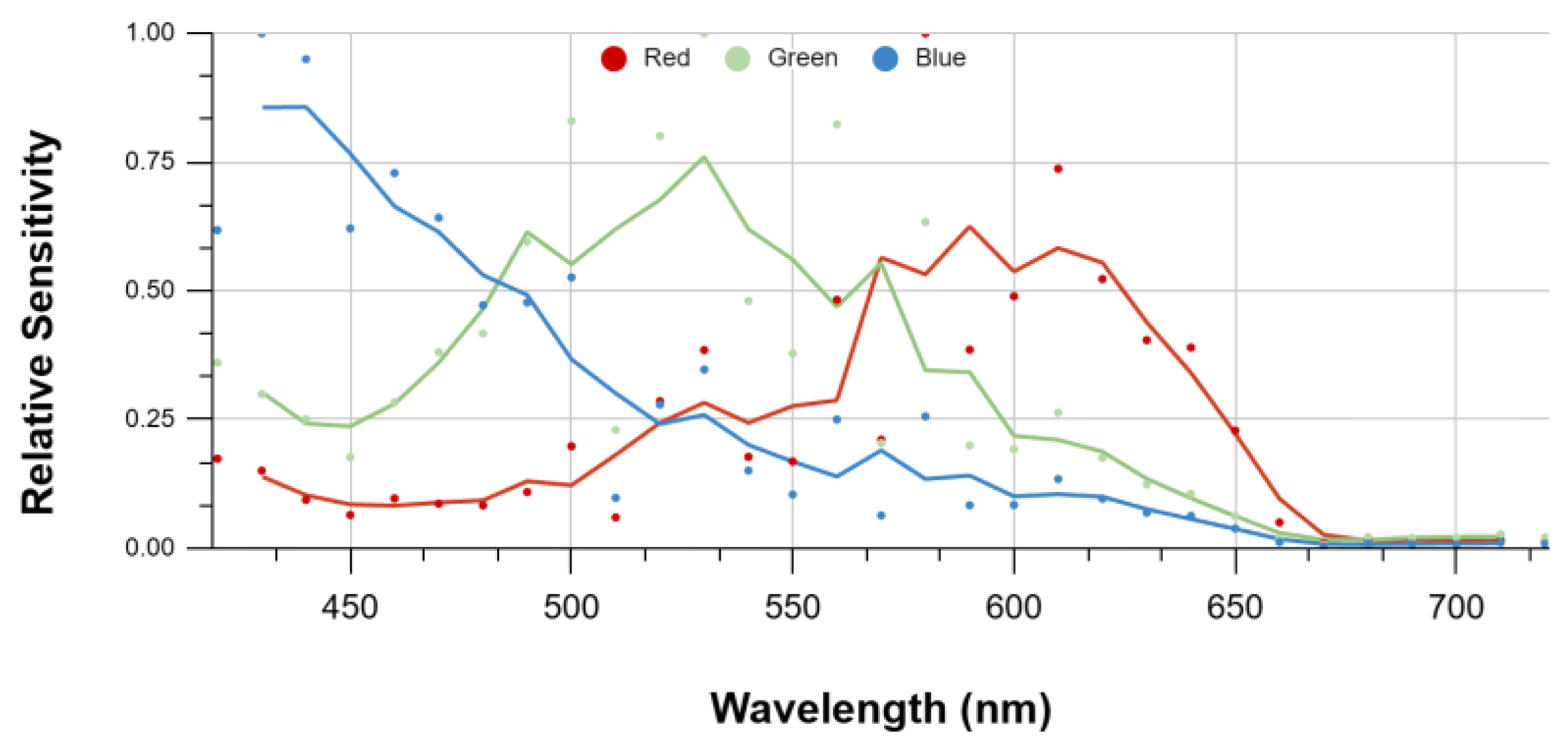
Figure 2.
Spectral transmittance of the Kurios XL1/M tunable filter as a function of wavelength. The points indicate experimentally measured values, while the continuous line corresponds to the fitted curve describing the spectral trend of the system.
Figure 2.
Spectral transmittance of the Kurios XL1/M tunable filter as a function of wavelength. The points indicate experimentally measured values, while the continuous line corresponds to the fitted curve describing the spectral trend of the system.
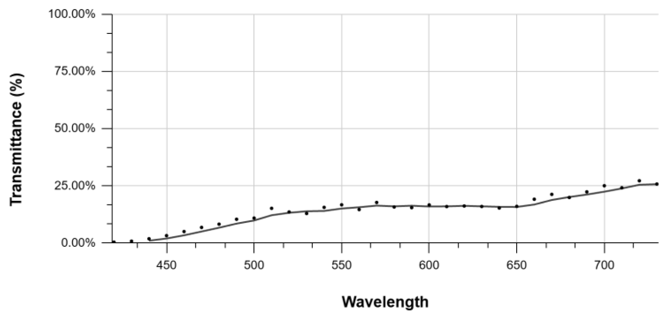
Figure 3.
Diagram of the acquisition system composed of a Blackmagic Camera, a Kurios tunable filter, and 50 mm and 100 mm optics, showing the arrangement of components.
Figure 3.
Diagram of the acquisition system composed of a Blackmagic Camera, a Kurios tunable filter, and 50 mm and 100 mm optics, showing the arrangement of components.
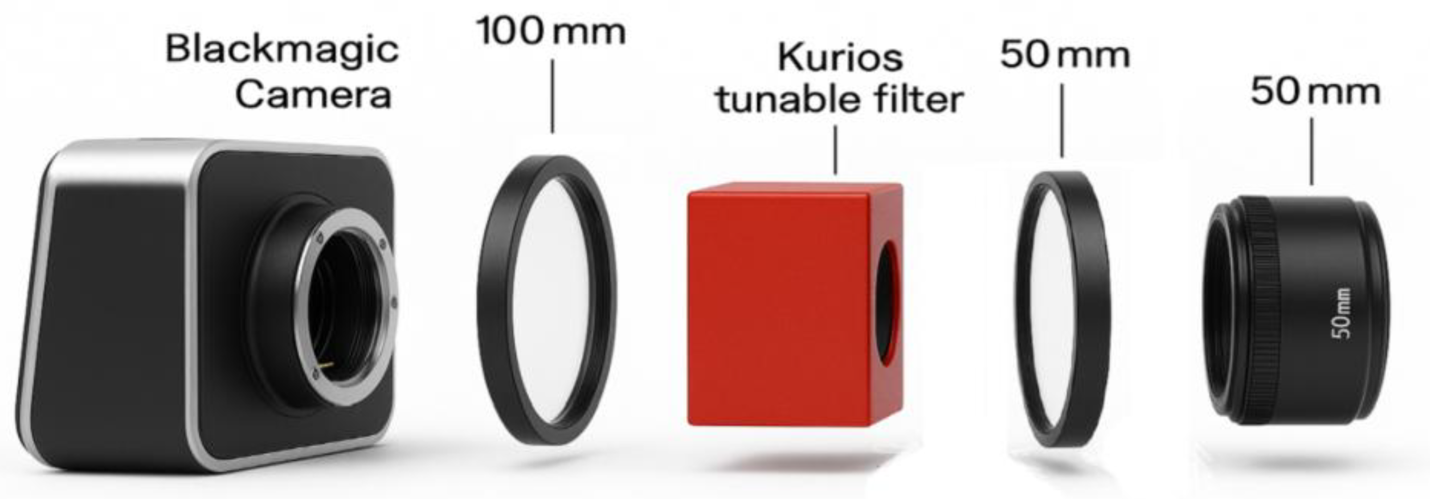
Figure 4.
Flow diagram of the proposed hyperspectral acquisition system. Scene radiance passes through the Kurios XL1/M tunable filter, whose spectral range is controlled by a software-generated signal transmitted as audio. This signal is recorded simultaneously with the sequence of raw images captured by the Blackmagic Cinema Camera 2.5K, enabling temporal correspondence between each frame and its associated spectral band. In parallel, a white reference is acquired for radiometric correction and reflectance measurement. Finally, the images are processed and reorganized to reconstruct the hyperspectral cube.
Figure 4.
Flow diagram of the proposed hyperspectral acquisition system. Scene radiance passes through the Kurios XL1/M tunable filter, whose spectral range is controlled by a software-generated signal transmitted as audio. This signal is recorded simultaneously with the sequence of raw images captured by the Blackmagic Cinema Camera 2.5K, enabling temporal correspondence between each frame and its associated spectral band. In parallel, a white reference is acquired for radiometric correction and reflectance measurement. Finally, the images are processed and reorganized to reconstruct the hyperspectral cube.
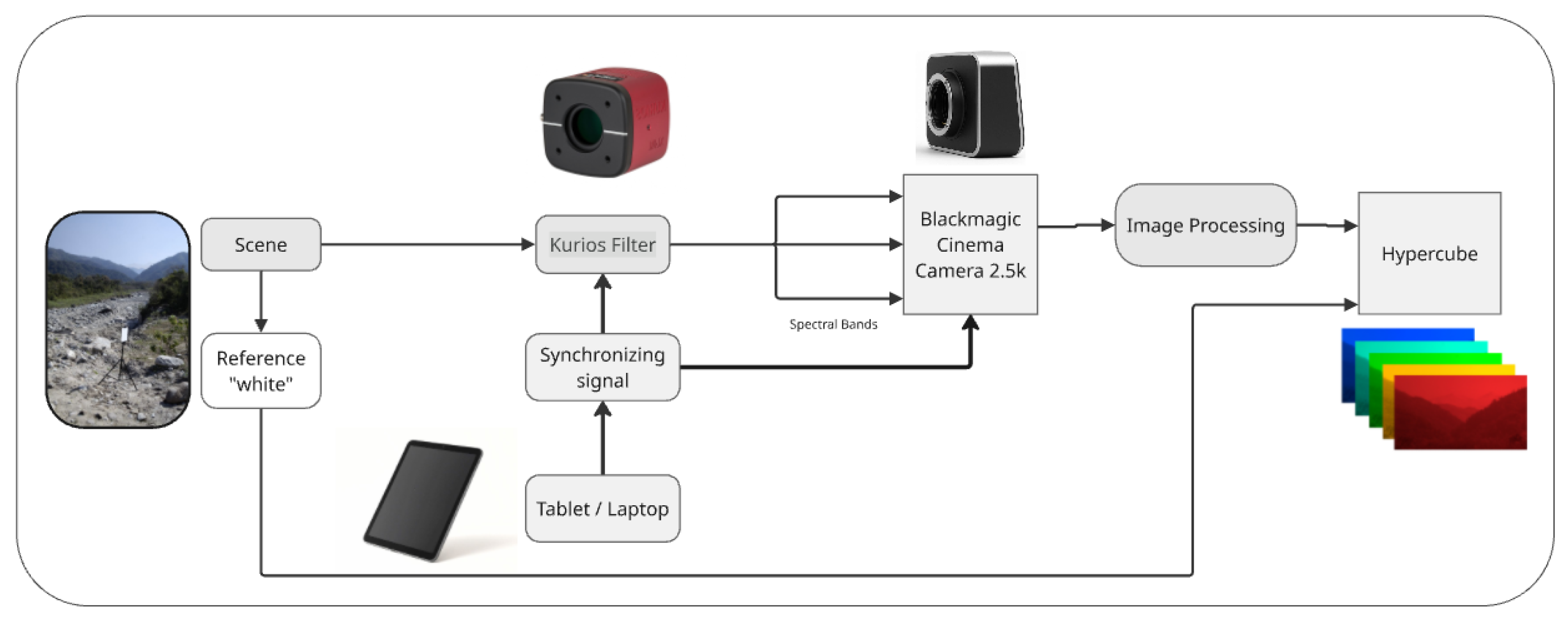
Figure 5.
Conceptual diagram of the acquisition synchronization system, in which a tablet sends a control signal that generates timed sound pulses associated with different spectral bands. These pulses are recorded by the camera (BMCC) to synchronize each image with its corresponding wavelength.
Figure 5.
Conceptual diagram of the acquisition synchronization system, in which a tablet sends a control signal that generates timed sound pulses associated with different spectral bands. These pulses are recorded by the camera (BMCC) to synchronize each image with its corresponding wavelength.
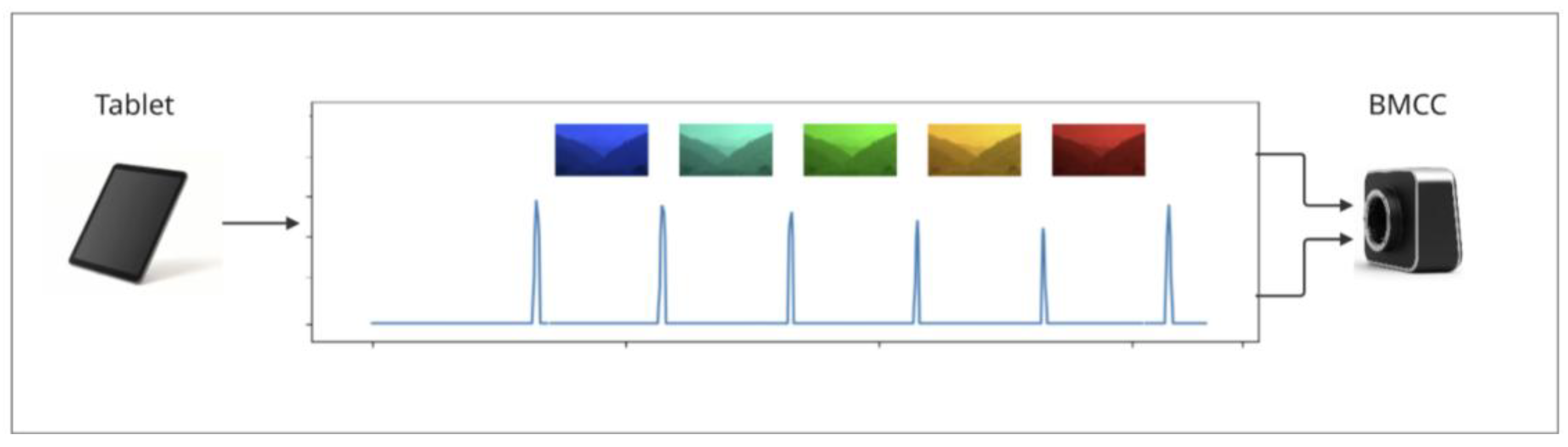
Figure 6.
Interface of the hyperspectral analysis software used for data visualization and processing. In the upper left, the scene image is displayed with the selected area of interest (red rectangle), corresponding to the analyzed region. In the lower left, the average spectral radiance curve of the selected area is shown as a function of wavelength, together with the standard deviation and minimum–maximum range. On the right, the spectral vectorscope is displayed, representing the chromatic distribution of radiance in angular coordinates associated with wavelength.
Figure 6.
Interface of the hyperspectral analysis software used for data visualization and processing. In the upper left, the scene image is displayed with the selected area of interest (red rectangle), corresponding to the analyzed region. In the lower left, the average spectral radiance curve of the selected area is shown as a function of wavelength, together with the standard deviation and minimum–maximum range. On the right, the spectral vectorscope is displayed, representing the chromatic distribution of radiance in angular coordinates associated with wavelength.
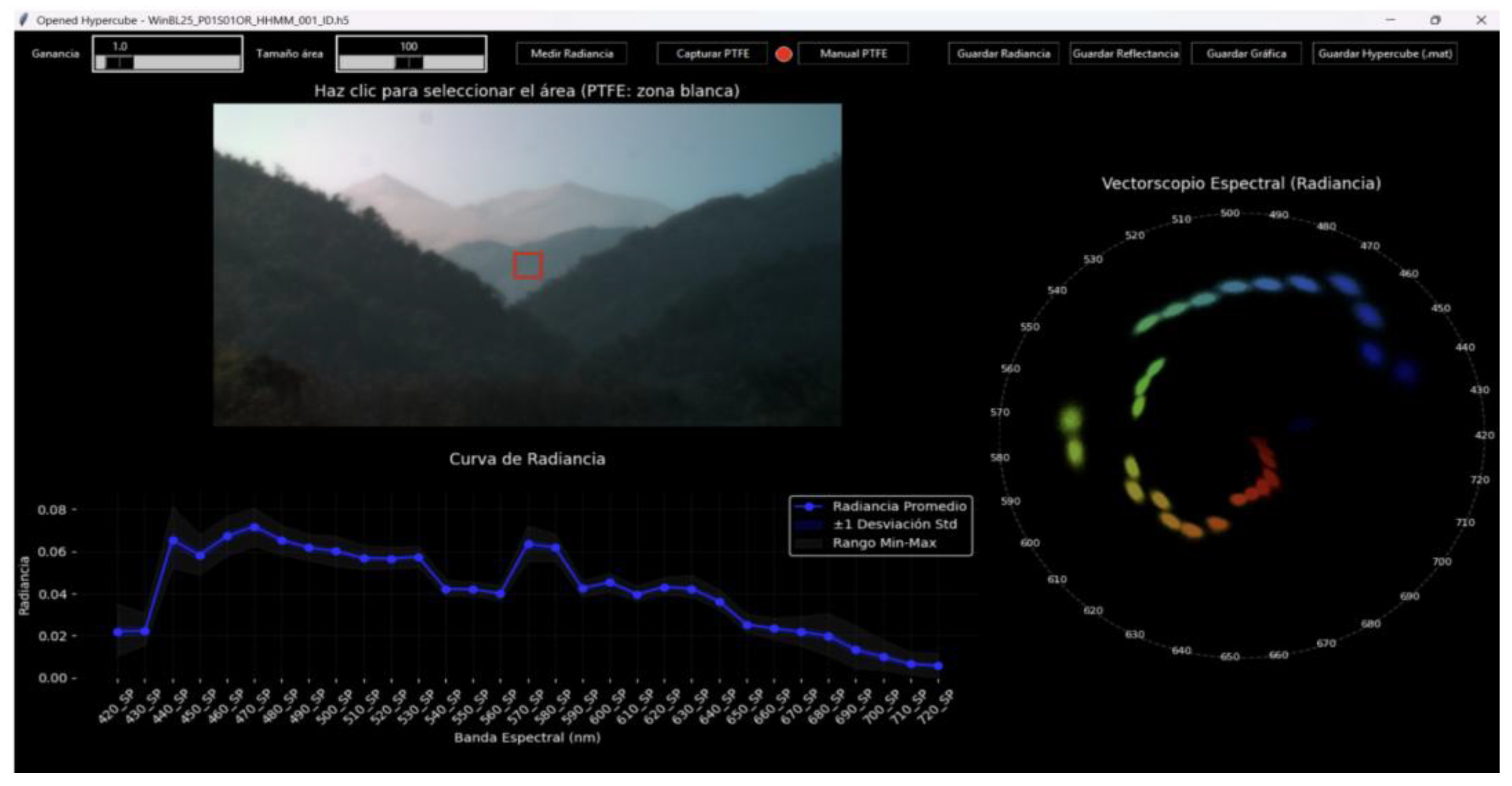
Figure 7.
Experimental setup for spectral data acquisition, consisting of a controlled illumination booth containing a color chart and black and PTFE samples inside.
Figure 7.
Experimental setup for spectral data acquisition, consisting of a controlled illumination booth containing a color chart and black and PTFE samples inside.
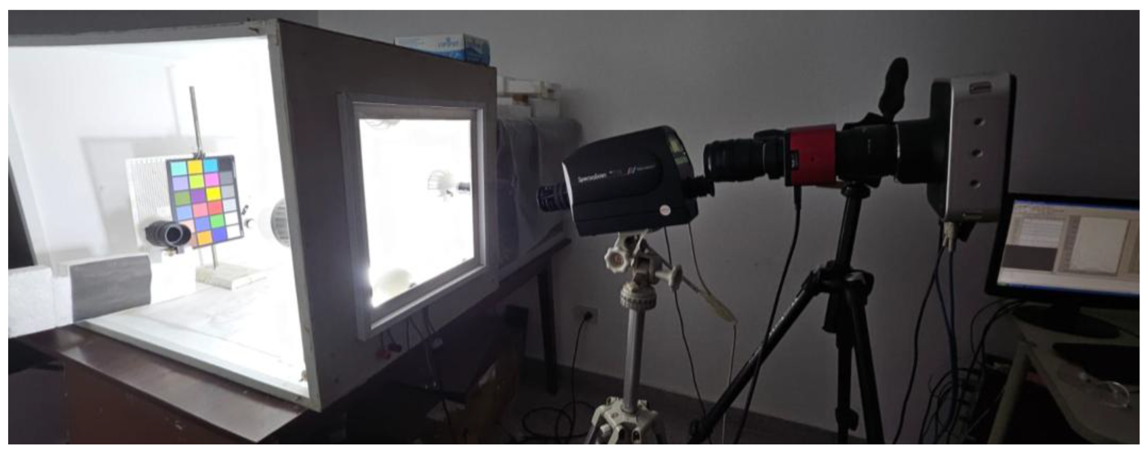
Figure 8.
(a) Experimental setup used to measure sensor linearity. (b) Relationship between the sensor’s digital signal (ADC) and the incident radiance measured at 540 nm, plotted on a logarithmic scale on both axes.
Figure 8.
(a) Experimental setup used to measure sensor linearity. (b) Relationship between the sensor’s digital signal (ADC) and the incident radiance measured at 540 nm, plotted on a logarithmic scale on both axes.
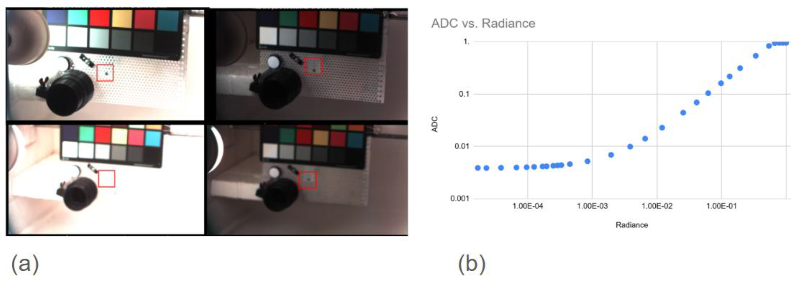
Figure 9.
Visualization of the original sample image (a), the homogeneity map Hmap (b), and the resulting corrected image (c).
Figure 9.
Visualization of the original sample image (a), the homogeneity map Hmap (b), and the resulting corrected image (c).
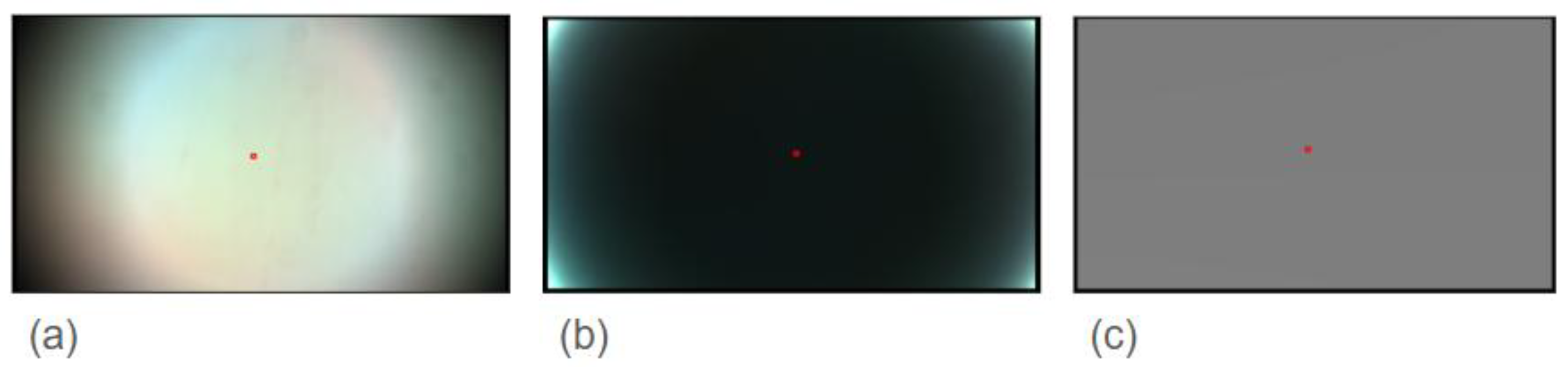
Figure 10.
Spectral percentage deviation between measurements obtained with the hyperspectral camera and reference spectroradiometer for different signal levels as a function of wavelength.
Figure 10.
Spectral percentage deviation between measurements obtained with the hyperspectral camera and reference spectroradiometer for different signal levels as a function of wavelength.
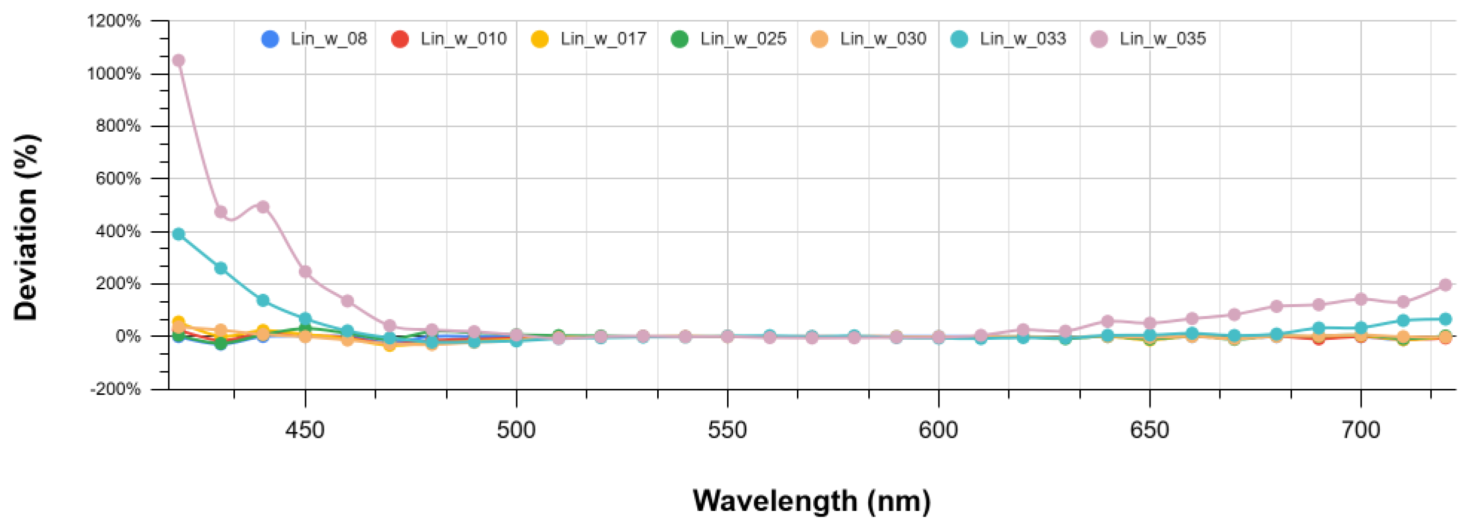
Figure 11.
Chromatic target used for the test (a) and spectral results obtained from its reflectance measurements (b), showing the correspondence between the measured object and the spectral signatures recorded by the system. Panel (a) shows the X-Rite color chart used as a reference pattern, composed of multiple chromatic patches arranged in a regular matrix, each with distinct reflective properties within the visible spectrum. Panel (b) displays the normalized spectral reflectance curves corresponding to the blue, green, red, yellow, magenta, and cyan patches of the color chart together with the PTFE reference. The horizontal axis represents wavelength (nm) and the vertical axis represents normalized reflectance. The curves exhibit characteristic spectral profiles for each color, indicating the direct relationship between the patches shown in (a) and their measured spectral responses in (b).
Figure 11.
Chromatic target used for the test (a) and spectral results obtained from its reflectance measurements (b), showing the correspondence between the measured object and the spectral signatures recorded by the system. Panel (a) shows the X-Rite color chart used as a reference pattern, composed of multiple chromatic patches arranged in a regular matrix, each with distinct reflective properties within the visible spectrum. Panel (b) displays the normalized spectral reflectance curves corresponding to the blue, green, red, yellow, magenta, and cyan patches of the color chart together with the PTFE reference. The horizontal axis represents wavelength (nm) and the vertical axis represents normalized reflectance. The curves exhibit characteristic spectral profiles for each color, indicating the direct relationship between the patches shown in (a) and their measured spectral responses in (b).
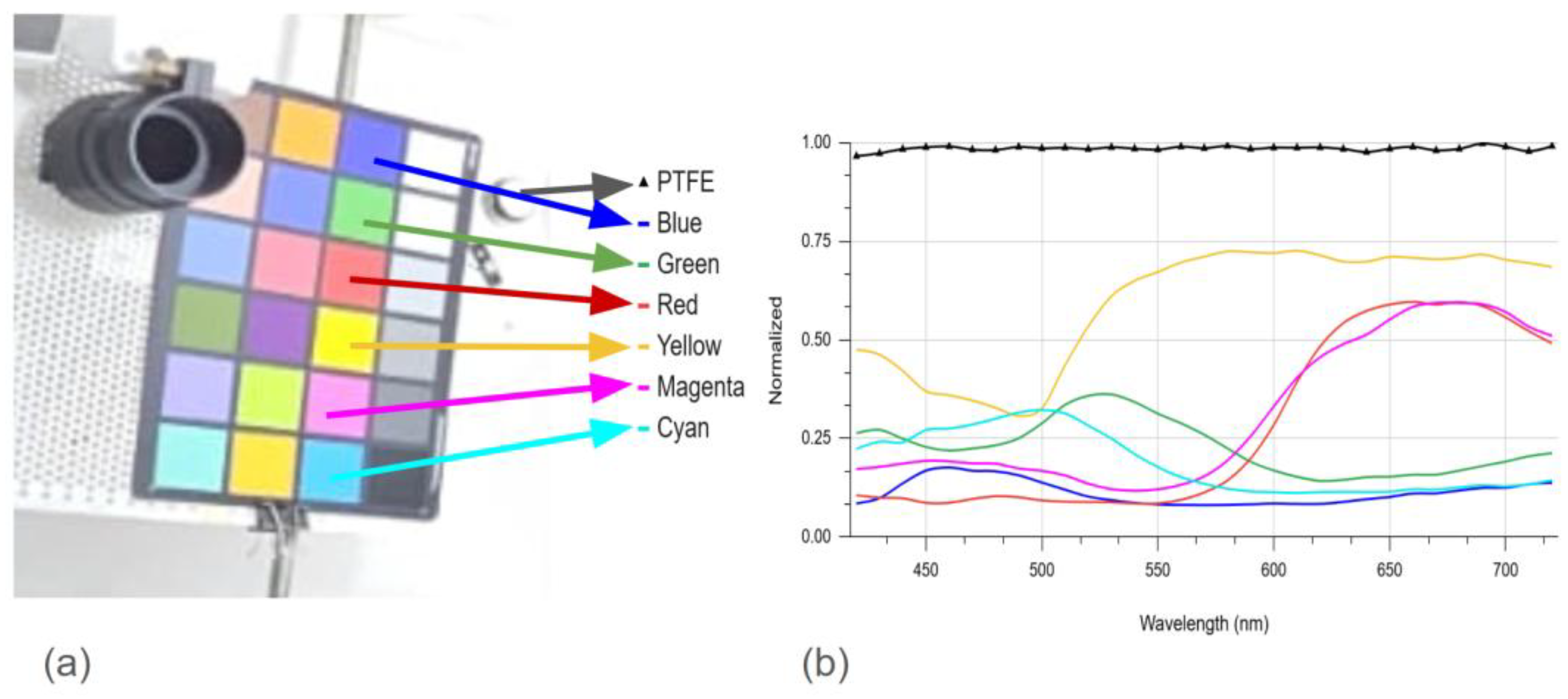
Figure 12.
(a) Hyperspectral system mounted inside the trunk of a car for field measurements. (b) Image of the hyperspectral system being controlled via a computer tablet.
Figure 12.
(a) Hyperspectral system mounted inside the trunk of a car for field measurements. (b) Image of the hyperspectral system being controlled via a computer tablet.
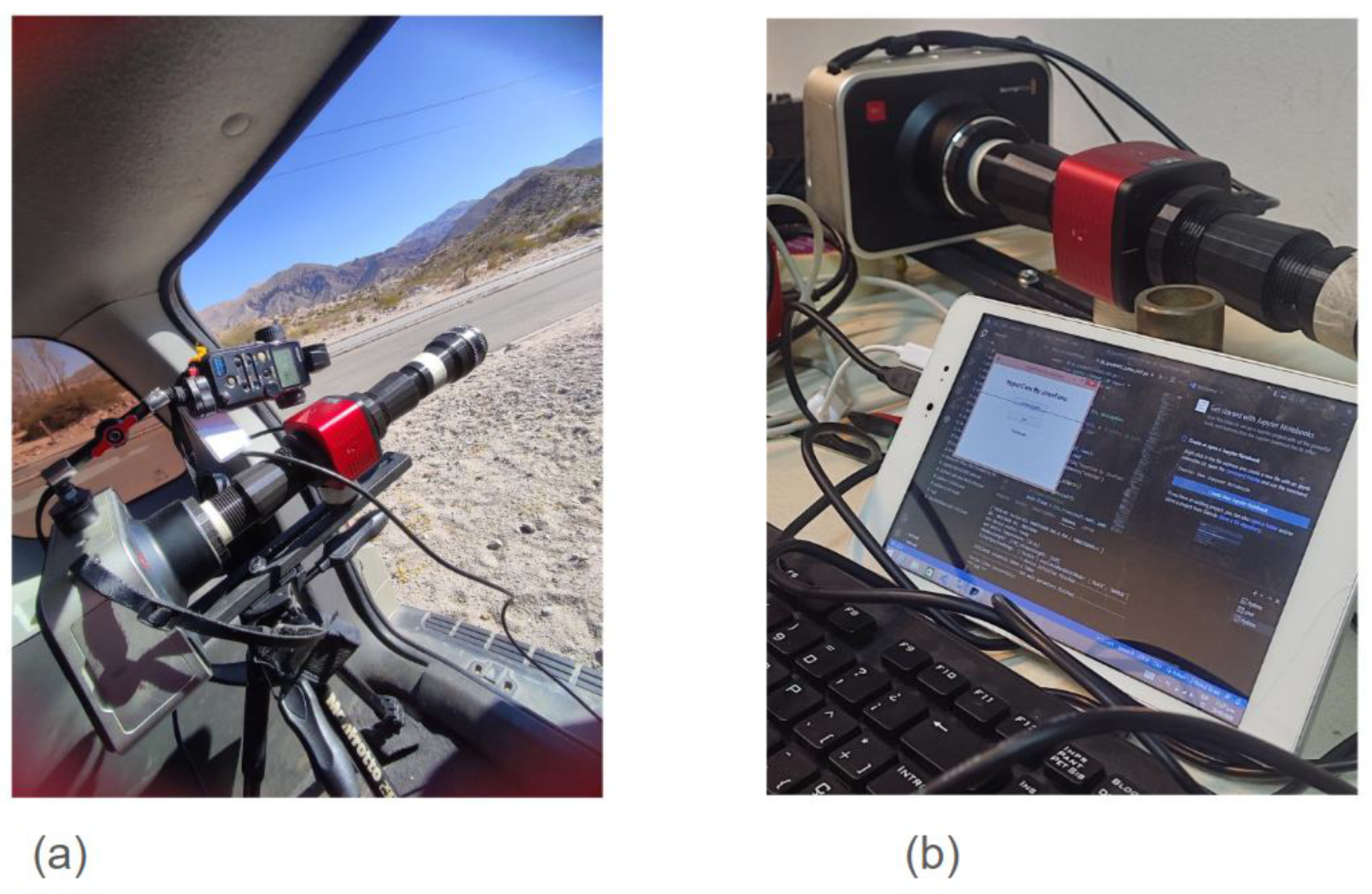

Table 1.
Comparison of spectral radiance at 540 nm measured with the hyperspectral camera and the spectroradiometer for different signal levels. Absolute radiance values (W·m⁻²·nm⁻¹) and the percentage difference between both systems are reported, both individually and as an average across the entire measured spectral range.
Table 1.
Comparison of spectral radiance at 540 nm measured with the hyperspectral camera and the spectroradiometer for different signal levels. Absolute radiance values (W·m⁻²·nm⁻¹) and the percentage difference between both systems are reported, both individually and as an average across the entire measured spectral range.
| Measurement | Spectral Radiance (W·m⁻²·nm⁻¹) at 540 nm | Difference | ||
|---|---|---|---|---|
| Developed Hyperspectral System | Photo Research Spectroradiometer | Individual | Average | |
| Lin_w_08 | 0.242 | 0.242 | 0.00% | -2.74% |
| Lin_w_010 | 0.0869 | 0.0866 | 0.35% | -2.53% |
| Lin_w_017 | 0.0274 | 0.0278 | -1.44% | -1.51% |
| Lin_w_025 | 0.00536 | 0.00537 | -0.19% | 1.33% |
| Lin_w_030 | 0.00172 | 0.00171 | 0.58% | -1.50% |
| Lin_w_033 | 0.00019 | 0.0002 | -5.00% | 32.65% |
| Lin_w_035 | 0.00008 | 0.00008 | 0.00% | 112.46% |
Disclaimer/Publisher’s Note: The statements, opinions and data contained in all publications are solely those of the individual author(s) and contributor(s) and not of MDPI and/or the editor(s). MDPI and/or the editor(s) disclaim responsibility for any injury to people or property resulting from any ideas, methods, instructions or products referred to in the content. |
© 2026 by the authors. Licensee MDPI, Basel, Switzerland. This article is an open access article distributed under the terms and conditions of the Creative Commons Attribution (CC BY) license (http://creativecommons.org/licenses/by/4.0/).
Copyright: This open access article is published under a Creative Commons CC BY 4.0 license, which permit the free download, distribution, and reuse, provided that the author and preprint are cited in any reuse.