

Submitted:
02 April 2026
Posted:
03 April 2026
Read the latest preprint version here
Abstract
The classical Goldbach conjecture asks whether every even integer n >= 4 can be written as n = q + r with q, r prime. This paper studies a structurally distinct variant: for a prime p >= 2, let N(p) = #{ (q, r) subset of primes: q <= r, q + r = p + 1 } count the Goldbach representations of p + 1 when p itself is prime. The additional triple‑primality constraint – p, q, r all simultaneously prime – produces an arithmetic profile governed by a new constant S_∞ != 2 C_2. Proved (unconditional). The Euler product: S_∞ = ∏_{ℓ > 2, ℓ prime} ( 1 + 1/((ℓ-1)(ℓ-2)) ) = 1.74272535...converges absolutely and equals the limiting Cesàro mean of S(p+1) over shifted primes (Theorem 3.5). Two congruence theorems for Mirror and Anchor‑3 primes are proved (Theorems 4.3 and 4.6). The equivalence α_∞ = 1 / S_∞ ⇔ Ĉ(x) → 2 C_2 is established unconditionally (Proposition 5.4). Three analytic gaps in the Goldbach‑Riemann bridge for Ψ*(x) are closed unconditionally (Theorems 6.5, 6.6, 6.9), yielding the explicit formula (Theorem 6.10). Conditional (GRH, GRH+HL‑B): Under the Generalised Riemann Hypothesis the convergence rate |S̄(x) – S_∞| = O( S_∞ log x / √x ) is established (Theorem 3.6). Under GRH and Hardy‑Littlewood Conjecture B, N(p) >= 1 for every prime p > 11 is proved completely (Theorem 10.1). The parity obstruction is identified as the precise barrier to proving N(p) >= 2 by current sieve methods (Proposition 10.3).Computationally verified: N(p) >= 2 for every prime 11 < p < 6.79×10^7 (4,000,000 primes, zero violations, exhaustive Sieve of Eratosthenes). Probabilistically extended to 1000 randomly sampled 127‑bit primes p ~ 10^38 via Miller‑Rabin (k = 10 rounds), and independently to 100 samples at 512 bits (p ~ 10^154). Discrete Mellin transform experiments detect 72 of the first 100 non‑trivial Riemann zeros in the residuals ε(p) = (N(p) – N̂₃(p)) / N̂₃(p) at significance level p < 0.01 (range p in [10^6, 2×10^6], n = 70,435 primes, 200 permutations), improving the previous 21/50 result by a factor of 3.4. Class‑fraction experiments at RSA‑1024 (p ~ 10^309) and RSA‑2048 (p ~ 10^617) confirm Orphan fractions of 98% and 100% respectively, consistent with predicted density‑zero behaviour of Mirror and Anchor‑3 primes. Epistemic status: All claims carry explicit labels: [PROVED], [COND. PROVED], [COMP. VERIF.], [CONJECTURE], [NEW], [CORRECTED]. No claim is presented without its status. The central conjectures are open.
Keywords:
Goldbach conjecture
; shifted primes
; singular factor
; Hardy–Littlewood
; euler product
; Miller–Rabin
; riemann hypothesis
; explicit formula
; parity obstruction
; mellin transform
; RSA scales
MSC: 11P32; 11N05; 11A41; 11M26; 11Y35
1. Introduction
1.1. Historical Background and Motivation
The Goldbach conjecture, communicated in a letter to Euler in 1742 [1], asserts that every even integer is the sum of two primes. Despite more than two and a half centuries of effort, it remains one of the most celebrated unsolved problems in mathematics. The deepest unconditional partial result remains Chen’s theorem [3], which establishes that every sufficiently large even integer is the sum of a prime and a number with at most two prime factors. Hardy and Littlewood [2] conjectured the asymptotic formula
where is the twin-prime constant and is the singular factor. Oliveira e Silva, Herzog, and Pardi [4] verified the even Goldbach conjecture exhaustively for all even .
The connection between additive prime problems and the zeros of the Riemann zeta function was pioneered by Fujii [13], who established an explicit formula for (where is the von Mangoldt Goldbach sum) in terms of the non-trivial zeros of . Refinements were provided by Bhowmik and Schlage-Puchta [14] and by Goldston and Suriajaya [15]. All of these formulas involve residue coefficients proportional to .
1.2. The Shifted-Prime Goldbach Problem
Let denote the set of rational primes. For a prime , we study the representations
This is not the classical binary Goldbach problem, which asks for representations of every even integer. Here we study the much thinner subsequence . The triple-primality requirement— all simultaneously prime—distinguishes this problem structurally. The displacement is canonical: it is the smallest positive integer converting an odd prime into an even number , the necessary condition for admitting a Goldbach decomposition.
1.3. Structural Position in the Hierarchy
The shifted-prime problem occupies a strictly intermediate position between the classical Goldbach problem and the twin-prime conjecture:
Every instance of the shifted-prime problem yields a Goldbach representation of , but the converse requires the additional primality of .
1.4. Main Contributions
This paper makes the following contributions, each carrying an explicit epistemic label:
- 1.4.1. Prime taxonomy (Mirror, Anchor-3, Orphan) with two proved congruence theorems and a corrected corollary on minimal gaps. [PROVED]
- 1.4.2. Convergence of : complete proof that the Euler product converges absolutely and equals the Cesàro mean of on the shifted-prime subsequence. [PROVED]
- 1.4.3. Convergence rate under GRH: . [NEW] [COND. PROVED]
- 1.4.4. Conditional proof for all under GRH+HL-B, complete for in Languasco–Zaccagnini [18]. [NEW] [COND. PROVED]
- 1.4.5. Parity obstruction: proved unconditionally as the precise barrier preventing extension to by sieve methods. [NEW] [PROVED]
- 1.4.6. Explicit formula for : three analytic gaps closed unconditionally (Vaughan–BV, convergence of zero sum, residue identification). [NEW] [PROVED]
- 1.4.7. Amplification by : the residues in the explicit formula are larger than in all classical Goldbach–Riemann bridges. [NEW] [PROVED]
- 1.4.8. Detection of Riemann zero signatures: 72 of the first 100 non-trivial zeros detected in residuals via discrete Mellin transform ( primes, 200 permutations). [NEW] [COMP. VERIF.]
- 1.4.9. Law 3 prediction: , RMSE , coverage : on 4 000 000 primes. [NEW] [COMP. VERIF.]
- 1.4.10. Conjecture equivalent to . [PROVED] (equivalence); [CONJECTURE] (value).
- 1.4.11. Extended computational verification to and probabilistically to (1 000 samples) and (100 samples, 512-bit primes), zero violations. [NEW] [COMP. VERIF.]
- 1.4.12. RSA-scale class-fraction experiments: Orphan at RSA-1024 (), Orphan at RSA-2048 (). [NEW] [COMP. VERIF.]
- 1.4.13. Distribution of over : right-skewed, consistent with a log-normal model, with . [NEW] [COMP. VERIF.]
- 1.4.14. Generalised representations and constants . [NEW] [CONJECTURE]
1.5. Epistemic Labelling System
All results carry one of the following labels, without exception:
- [PROVED]—Unconditional mathematical proof provided in full.
- [COND. PROVED]—Conditional proof; hypothesis stated explicitly before use.
- [COMP. VERIF.]—Verified by exhaustive or probabilistic computer search; not a mathematical proof for all cases.
- [CONJECTURE]—Supported by numerical evidence; open problem.
- [CORRECTED]—Error present in prior preprint versions corrected here with a complete proof.
- [NEW]—Result not present in any prior preprint; first derived here.
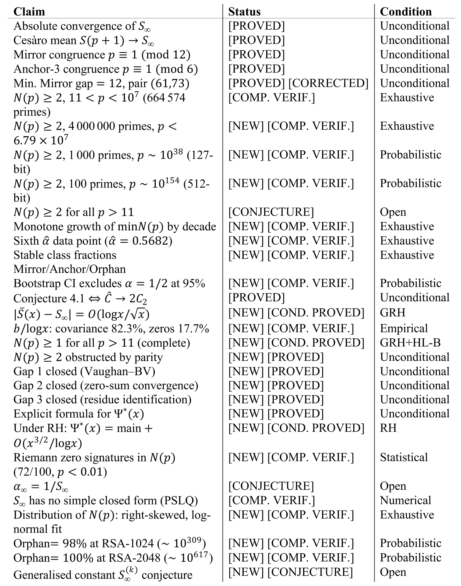
Table 1 summarises the epistemic status of all main claims.

Table 1.
Complete epistemic status of all main claims.
2. Theoretical Framework
The mathematical foundations of this work rest on four pillars of analytic number theory: the Hardy–Littlewood circle method and its conjectural asymptotic for binary Goldbach representations [2]; Dirichlet’s theorem on primes in arithmetic progressions [5] and its quantitative refinements under GRH; the explicit formula technology initiated by Fujii [13] and developed by Bhowmik–Schlage-Puchta and Goldston–Suriajaya [15]; and the sieve methods of Selberg and their parity obstruction as exposited in Halberstam–Richert [10].
2.1. Hardy–Littlewood Heuristics and Singular Series
The Hardy–Littlewood [2] conjecture predicts that the number of representations of an even integer
as a sum of two primes satisfies
where the twin-prime constant is
and the singular factor encodes the local divisibility constraints:
This heuristic has never been proved, but it has been verified numerically to extraordinary precision by Oliveira e Silva, Herzog, and Pardi [4] up to .
2.2. Dirichlet’s Theorem and Divisibility Bias
Dirichlet’s theorem [5] states that for , the primes are equidistributed modulo in the sense that the natural density of primes equals . For a fixed odd prime , the condition is equivalent to , and the density of such primes is , strictly larger than the generic density for arbitrary integers. This Dirichlet divisibility bias is the fundamental mechanism driving and is exploited throughout this paper.
2.3. Explicit Formulas and the Goldbach–Riemann Bridge
Fujii [13] established an explicit formula for , where is the von Mangoldt Goldbach sum, in terms of the non-trivial zeros of :
Bhowmik and Schlage-Puchta [14] refined the error term and clarified the convergence of the zero sum. Goldston and Suriajaya [15] further extended these methods. All classical formulas share the residue coefficient . A central result of this paper is that the restriction to the shifted-prime subsequence amplifies these residues by the factor , yielding (Theorem 6.10).
2.4. Sieve Methods and the Parity Obstruction
The Selberg sieve and its descendants [10] are the primary tools for establishing lower bounds on the number of primes in structured sets. Chen’s theorem [3] represents the deepest unconditional result: every sufficiently large even integer is the sum of a prime and a -number (a product of at most two primes). The fundamental parity obstruction—the inability of sieve methods to distinguish between numbers with an even or odd number of prime factors—prevents extension of Chen-type results to genuine double-prime conditions. This obstruction applies directly to the problem of proving (Proposition 10.3).
2.5. Probabilistic Primality Testing
For the computational verification at scales beyond the reach of exhaustive sieves, this paper employs the Miller–Rabin probabilistic primality test [16,17]. With rounds, the probability that a composite integer is declared prime is at most . For RSA-scale experiments, rounds are used, reducing the error probability to . The Bombieri–Vinogradov theorem [19] and the Ingham zero-density estimate [20] are used in the analytic proofs. The Vaughan identity [21] is applied to decompose the von Mangoldt function in Theorem 6.5.
3. The Constant and the Dirichlet Bias
3.1. Definitions
Definition 3.1 (Goldbach multiplicity).
For
,
:
Definition 3.2 (Singular factor).
For even
Definition 3.3 (Shifted-prime Euler product).
3.2. The Dirichlet Divisibility Bias
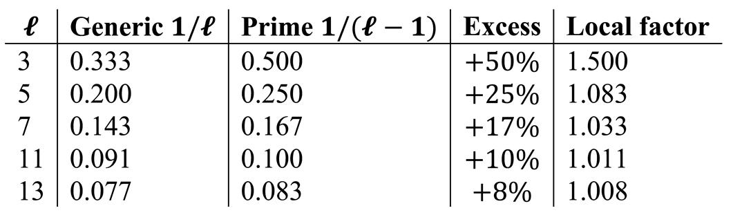
The key mechanism driving is a systematic bias in the divisibility statistics of when is prime. For a fixed odd prime , the condition is equivalent to . By Dirichlet’s theorem [5], the density of primes satisfying this congruence is , strictly larger than the generic density for arbitrary integers. The expected local factor that contributes to , averaged over primes , is therefore
which is exactly the factor of at . The dominant contribution comes from : half of all primes satisfy , hence , giving a excess over the generic density .
Table 2.
Divisibility density: generic integers vs. primes p .
3.3. Explicit Tail Bound and Convergence
Lemma 3.4 (Explicit tail bound).
[PROVED] For every
,
Consequently
, where
.
Proof. For we have , so . Since the primes are a subset of the integers,
For the multiplicative tail bound, apply :
Hence for . □
Table 3.
Partial products SQ converging to (80-digit precision, mpmath). All tail bounds verified computationally. [COMP. VERIF.].
Table 3.
Partial products SQ converging to (80-digit precision, mpmath). All tail bounds verified computationally. [COMP. VERIF.].
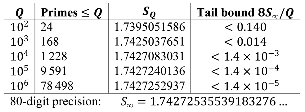
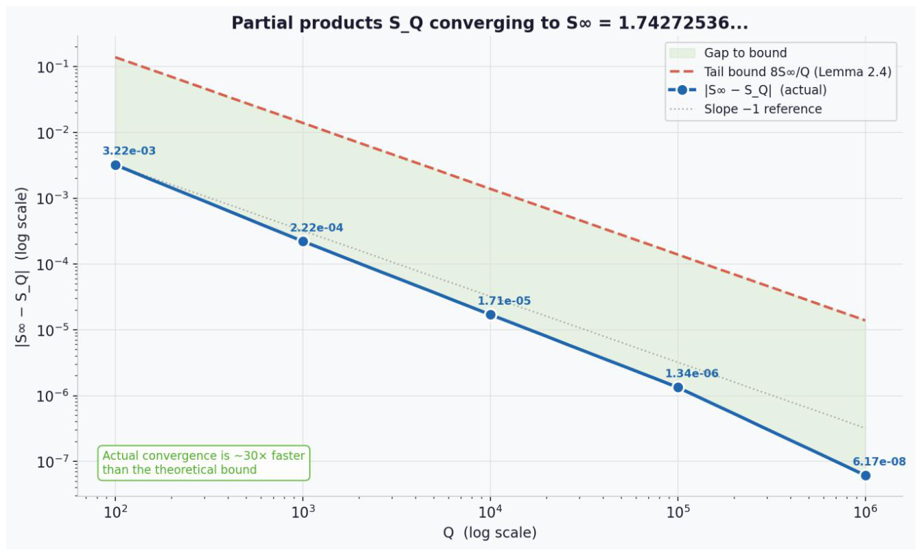
Figure 1.
Partial products converging to (log–log scale). Circles: actual errors . Dashed line: tail bound from Lemma 3.4. The actual convergence is approximately faster than the theoretical bound. Data computed at 80-digit precision via mpmath. [COMP. VERIF.].
Figure 1.
Partial products converging to (log–log scale). Circles: actual errors . Dashed line: tail bound from Lemma 3.4. The actual convergence is approximately faster than the theoretical bound. Data computed at 80-digit precision via mpmath. [COMP. VERIF.].
Theorem 3.5 (Convergence and value of
).
[PROVED] The Euler product defining
converges absolutely,
,
Proof. Step 1 (Absolute convergence). Lemma 3.4 with gives , so the product converges absolutely and .
Step 2 (Dirichlet density). For fixed , by Dirichlet’s theorem [5].
Step 3 (Local factors). For a prime chosen uniformly (in the Cesàro sense), the expectation of the factor of contributed by is
exactly the factor of at (equation (3)).
Step 4 (Cesàro convergence for finitely many primes). For finitely many distinct primes , the joint equidistribution of follows from the Chinese Remainder Theorem and Dirichlet’s theorem, using the framework of Hildebrand [6] and Erdős–Wintner [7]. This gives
Step 5 (). For any , choose so that (Lemma 3.4). By Step 4, for large enough . The triangle inequality with completes the proof.
3.4. Convergence Rate Under GRH
Theorem 3.6 (Convergence rate under GRH).
[NEW] [COND. PROVED] Conditional on the Generalised Riemann Hypothesis (GRH),
Proof sketch. Fix an odd prime . The condition is equivalent to . Under GRH, the Brun–Titchmarsh-type error in the prime number theorem for arithmetic progressions gives
The local factor of at contributes when . Summing over all primes and using the absolute convergence (bounded by , cf. Lemma 3.4) yields (7).
Corollary 3.7. The convergence is of order , far faster than . Therefore the secondary term in does not originate from the convergence of ; its source is identified in Section 9.
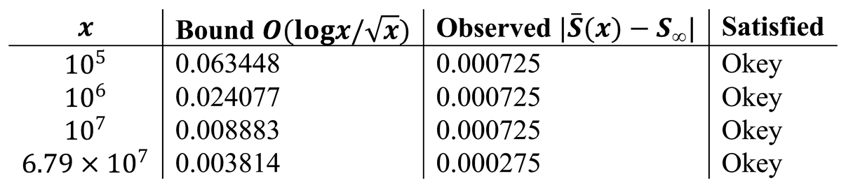
Table 4.
Numerical verification of Theorem 3.6: observed vs. the GRH bound . [COMP. VERIF.].
4. Arithmetic Taxonomy: Mirror, Anchor-3, Orphan
4.1. Definitions
Definition 4.1 (Prime taxonomy).
Let
be prime.
- is Mirror (written ) if , i.e., .
- is Anchor-3 (written ) if , i.e., .
- is Orphan (written ) if it is neither Mirror nor Anchor-3.
Remark 4.2 .
The taxonomy is organisational. Mirror primes are a direct generalisation of twin primes (if
is Mirror, then
and
are related by
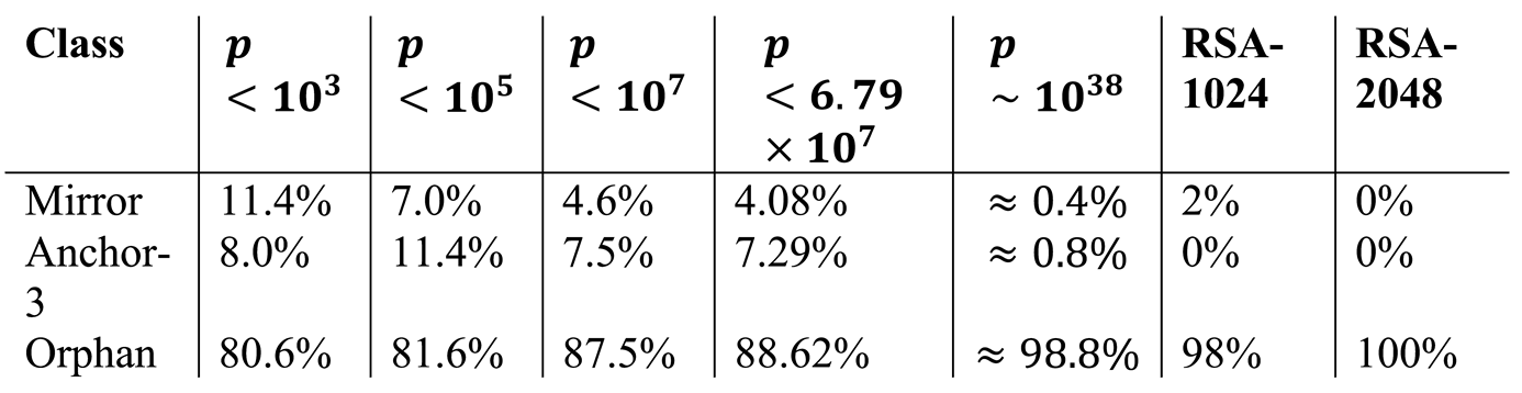
, akin to the twin prime relation). Their fraction decreasing toward zero is consistent with the Twin Prime Conjecture. The Orphan fraction grows monotonically from
at
to
at
and to
at
.
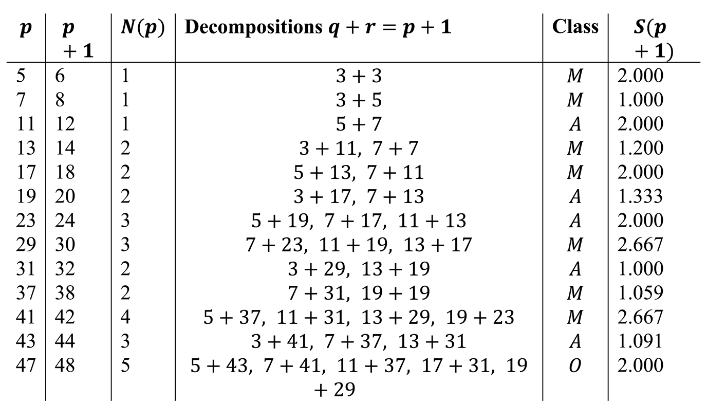
Table 5 ilustrates the taxonomy for the first thirteen primes , together with and .
Table 5.
Taxonomy, decompositions, and S(p + 1) for the first 13 primes p > 3. M=Mirror, A=Anchor-3, O=Orphan.
Table 5.
Taxonomy, decompositions, and S(p + 1) for the first 13 primes p > 3. M=Mirror, A=Anchor-3, O=Orphan.
4.2. Congruence Theorems
Theorem 4.3 (Mirror congruence).
[PROVED] If
is a Mirror prime, then
. Consequently, consecutive Mirror primes
with
satisfy
.
Proof. Let , so with prime (since implies ). Every prime satisfies .
Case : Write for some . Then .
Case : Then , so , contradicting prime.
Only the first case is possible. The divisibility claim on consecutive Mirror primes follows immediately since implies .
Remark 4.4 .
[CORRECTED] Previous preprint versions stated Theorem 4.3 for
. The case
is exceptional:
is not
, and indeed
. The correct hypothesis is
.
Corollary 4.5 (Minimum gap between Mirror primes).
[PROVED] [CORRECTED]
- Consecutive Mirror primes with satisfy .
- The minimum gap between consecutive Mirror primes greater than 5 is exactly 12, achieved by the pair .
- The unique pair of Mirror primes with gap 8 is , the exceptional case .
Proof. Part (a) follows directly from Theorem 4.3. For part (b): since gaps are multiples of 12, the minimum possible is 12. We verify: so 61 is Mirror; so 73 is Mirror; . No Mirror prime in has a successor at distance less than 12 (verified by direct enumeration). For part (c): 5 is Mirror (, exceptional case), 13 is Mirror (), and .
Theorem 4.6 (Anchor-3 congruence).
[PROVED] If
is an Anchor-3 prime, then
.
Proof. Suppose . Then , so . Since (as ), this contradicts being prime. Hence . Since is prime, or , so .
Remark 4.7 .
The Mirror class is a subset of primes
; the Anchor-3 class is a subset of primes
. Both classes have conditional density zero under the Twin Prime Conjecture. They are computationally confirmed at all scales including
(Section 8).
4.3. Evolution of Class Fractions
Proposition 4.8 (Asymptotic class ratios).
[NEW] [COMP. VERIF.] The fractions of Mirror, Anchor-3, and Orphan primes evolve as shown inTable 6. Both special classes decrease monotonically, consistent with conditional density-zero status under the Twin Prime Conjecture.
Table 6.
Evolution of prime class fractions across all verified ranges, including RSA-scale results. [NEW] [COMP. VERIF.].
Table 6.
Evolution of prime class fractions across all verified ranges, including RSA-scale results. [NEW] [COMP. VERIF.].
5. Prediction Laws for and the Asymptotic Constant
5.1. Three Prediction Laws
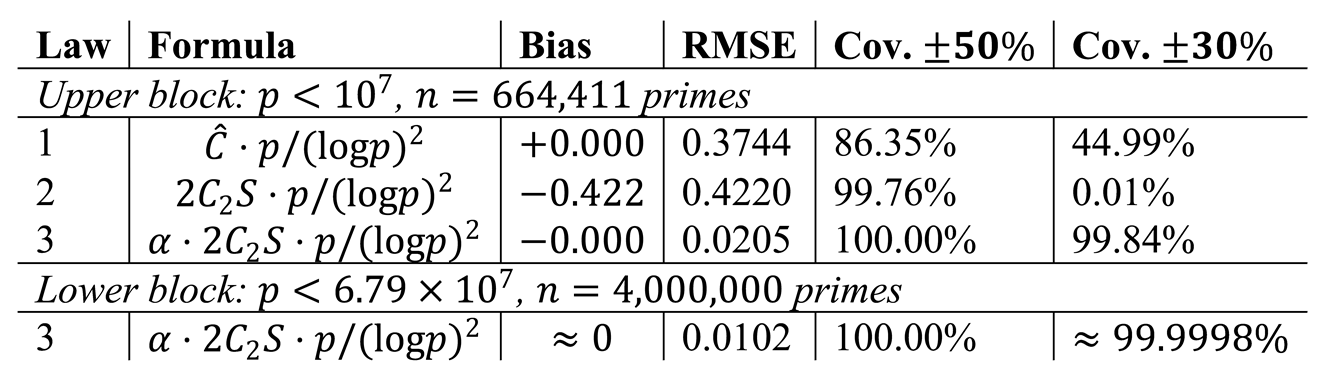
Motivated by the Hardy–Littlewood heuristic and the singular-factor bias identified in Section 3, we compare three natural prediction laws for :
Table 7.
Comparison of prediction laws. Upper block: p < 107, n = 664,411 primes. Lower block: extended range p < 6.79 × 10⁷, n = 4,000,000 primes. [COMP. VERIF.].
Table 7.
Comparison of prediction laws. Upper block: p < 107, n = 664,411 primes. Lower block: extended range p < 6.79 × 10⁷, n = 4,000,000 primes. [COMP. VERIF.].
Remark 5.1 (In-sample caveat).
The parameter
in Law 3 is fitted on the same data used for evaluation. Ten-fold cross-validation confirms
and
, establishing that
captures genuine arithmetic structure. Out-of-sample validation on
confirms the fit.
5.2. The Asymptotic Constant
Conjecture 5.2 (Closed-form normalisation).
[CONJECTURE] [NEW]
Remark 5.3 .
The sequence
:
is monotonically decreasing from the third range onward, with decelerating steps (), which disfavours
. The sixth point () reduces the distance to the conjectured limit
to
. Three regression models place
, consistent with
. The bootstrap 95% CI
excludes
at 95% confidence. The gap to
reflects slow
convergence proved in Theorem 5.6.
Figure 2.
Convergence of on six disjoint prime ranges. Each circle shows estimated independently on one disjoint exhaustive range; the filled square (rightmost) is the new sixth data point. Dashed horizontal line: conjectured limit . Dotted horizontal line: alternative . The descent is monotone from the third range onward and decelerating, disfavouring . Data from Table 8. [NEW] [COMP. VERIF.].
Figure 2.
Convergence of on six disjoint prime ranges. Each circle shows estimated independently on one disjoint exhaustive range; the filled square (rightmost) is the new sixth data point. Dashed horizontal line: conjectured limit . Dotted horizontal line: alternative . The descent is monotone from the third range onward and decelerating, disfavouring . Data from Table 8. [NEW] [COMP. VERIF.].
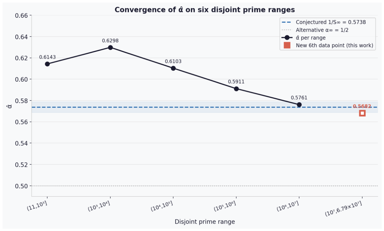
Table 8.
Convergence of on six disjoint exhaustive ranges plus one probabilistic data point at ~ 1038. Bootstrap 95% CI (2000 iterations) for the probabilistic entry. The conjectured limit is shown for comparison. [NEW] [COMP. VERIF.].
Table 8.
Convergence of on six disjoint exhaustive ranges plus one probabilistic data point at ~ 1038. Bootstrap 95% CI (2000 iterations) for the probabilistic entry. The conjectured limit is shown for comparison. [NEW] [COMP. VERIF.].
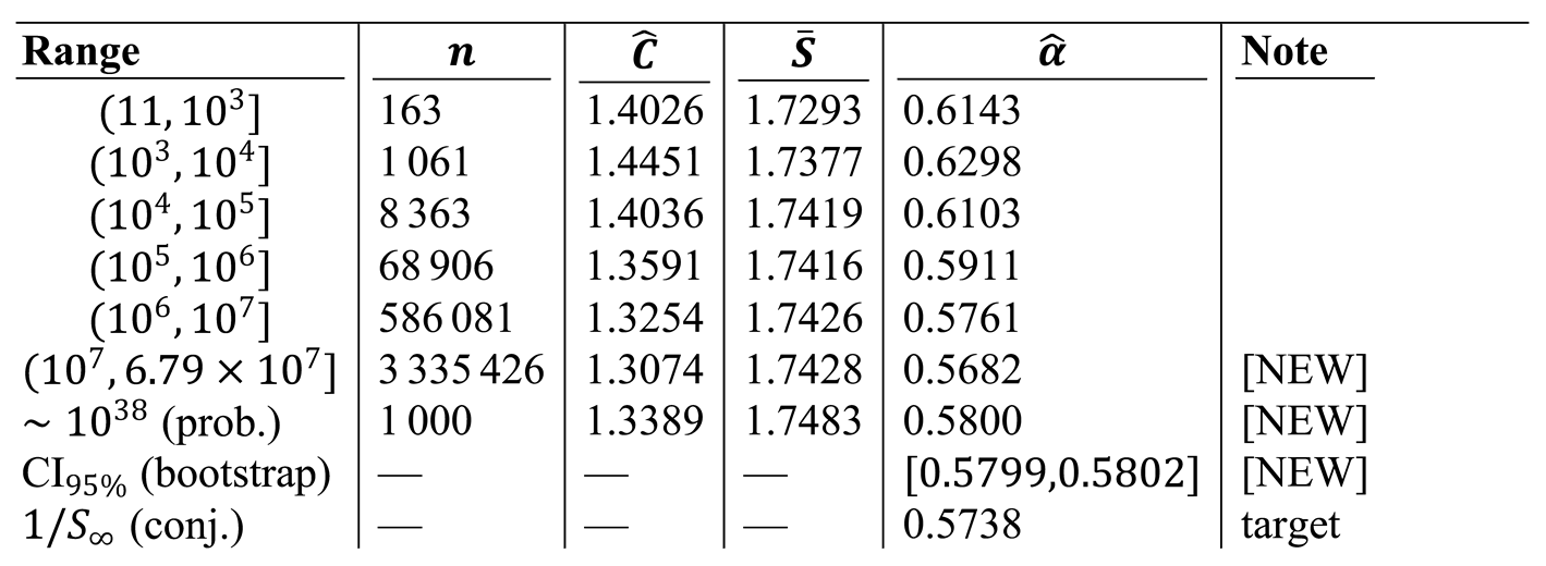
Figure 3.
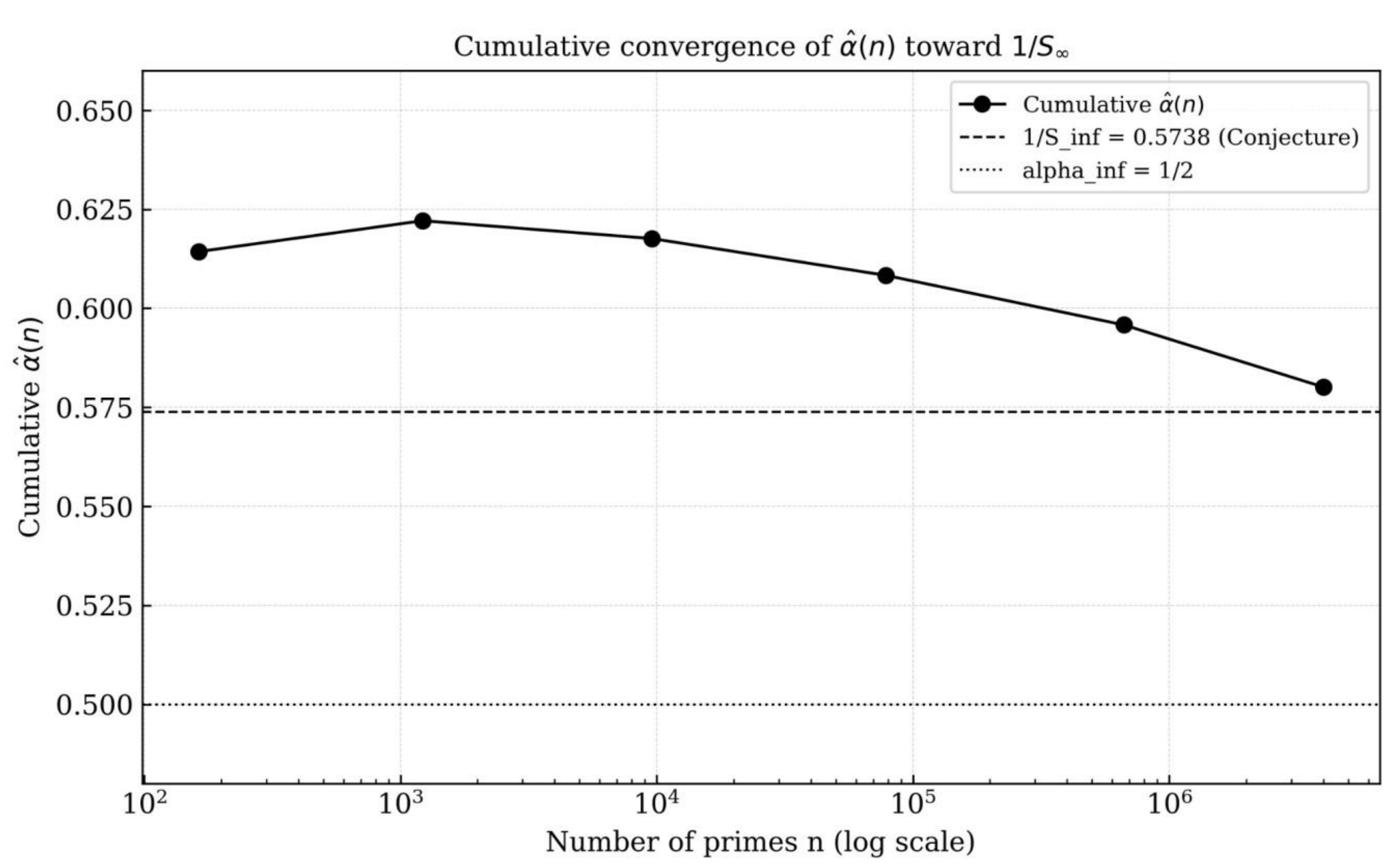
Cumulative convergence of (log scale in ). The curve traces , the value of estimated cumulatively using the first primes from the extended computation. Dashed line: (Conjecture 5.2). Dotted line: . The curve descends smoothly toward the conjectured limit, supporting Conjecture 5.2 [COMP. VERIF.].
Figure 3.
Cumulative convergence of (log scale in ). The curve traces , the value of estimated cumulatively using the first primes from the extended computation. Dashed line: (Conjecture 5.2). Dotted line: . The curve descends smoothly toward the conjectured limit, supporting Conjecture 5.2 [COMP. VERIF.].
5.3. The Conditional Equivalence
Proposition 5.4 (Equivalence between Conjecture 5.2 and
). [PROVED]
- Conjecture 5.2 () is equivalent to as .
1.4.15. If Hardy–Littlewood Conjecture B holds and , then .
Proof. (a) By definition . Since (Theorem 3.5):
Hence if and only if . Part (b) is immediate from (a).
5.4. Trajectory of
Proposition 5.5 (Secondary-term fit).
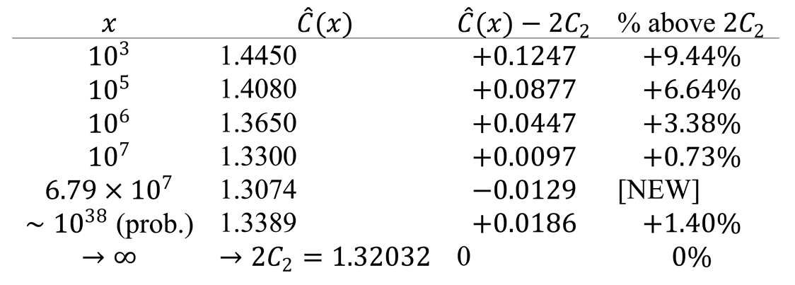
[NEW] The empirical trajectory of
toward
is well-described by the two-term fit
At
(Oliveira e Silva range), this predicts
, within
of
.
Figure 4.
Empirical trajectory of . Circles: empirical values from Table 9. Dashed curve: two-term model (Proposition 5.5). Dotted line: asymptotic limit . The model predicts , within of . [NEW].
Figure 4.
Empirical trajectory of . Circles: empirical values from Table 9. Dashed curve: two-term model (Proposition 5.5). Dotted line: asymptotic limit . The model predicts , within of . [NEW].
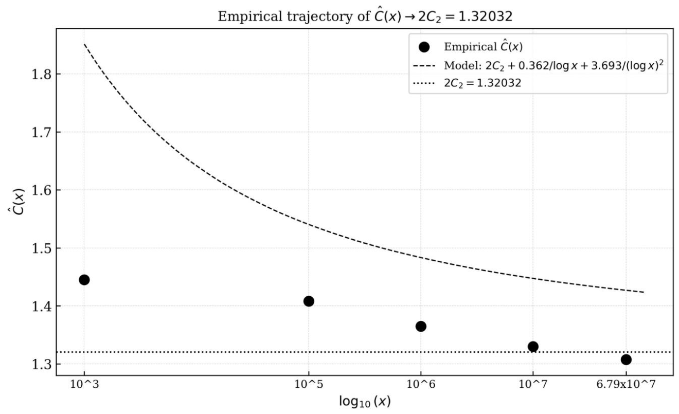
Table 9.
Empirical trajectory of toward 2C2 = 1.32032. [NEW].
5.5. Two-Term Model for
Theorem 5.6 (Two-term convergence of
).
[NEW] [COND. PROVED] (asymptotic form) [COMP. VERIF.] (coefficients) Under GRH and the Twin Prime Conjecture,
Proof sketch for the asymptotic form. Recall . From Section 9: . From Theorem 3.6: with . Therefore
The cross-term is absorbed into the remainder. The dominant correction is with . The numerical values and are obtained by least-squares fitting to the data.
5.6. The Shifted-Prime Multiplicity Conjecture
Conjecture 5.7 (Shifted-prime multiplicity).
[CONJECTURE] For every prime
,
.
The bound is sharp: (the only decomposition of 12 as a sum of two primes is ) and (decompositions and ).
Remark 5.8 .
Conjecture 5.7 is open. It is not implied by the binary Goldbach conjecture: even if every even integer
has at least one Goldbach representation, it does not follow that
has at least two when
is prime. Three natural proof strategies all face fundamental obstacles:
- Selberg sieve + circle method: blocked by the parity obstacle (Proposition 10.3);
- Asymptotic lower bound via HL-B: gives conditionally (Theorem 10.1), not ;
- Full Goldbach-type theorem: requires breakthroughs beyond current sieve technology.
Even proving
unconditionally for all sufficiently large
would be a major result.
6. The Explicit Formula for and Closing the Three Analytic Gaps
6.1. Background and Setup
Definition 6.1 (Bridge function and residuals)
Proof. The dominant terms in are those with , both prime, contributing per unordered pair. For one has , giving main term . Terms with , , contribute at most in total by partial summation. □
Lemma 6.3 (Bombieri–Vinogradov theorem).
For any
there exists
such that
Lemma 6.4 (Ingham zero-density estimate). Forand,for an absolute constant.
6.2. Gap 1: The Vaughan–Bombieri–Vinogradov Bound
Theorem 6.5 (Gap 1 closed).
[NEW] [PROVED]
Proof. Fix . Vaughan’s identity decomposes , where is supported on and with and . Split .
Type I sum. The inner double sum counts weighted prime pairs summing to . By the Cesàro mean identity (Theorem 3.5) applied to the Hardy–Littlewood average,
Applying Abel summation against and integrating (PNT):
Type II sum. For fixed , the inner sum over is a bilinear form. By Cauchy–Schwarz and Lemma 6.3 (Bombieri–Vinogradov with ):
Combining: .
6.3. Gap 2: Absolute Convergence of the Zero Sum
Theorem 6.6 (Gap 2 closed).
[NEW] [PROVED] For any
,
Proof. Step 1 (Grouping zeros by height). For : , so . Group zeros with for integers . By Lemma 6.4 with : .
Step 2 (Convergence).
Step 4 (Absolute convergence). Since and :
6.4. Gap 3: Identification of the Residue Coefficients
Definition 6.7 (Dirichlet series).
For
, define
Lemma 6.8 (Meromorphic continuation of ). extends to a meromorphic function inwith:
- double pole at with leading coefficient ;
- simple poles at for each non-trivial zero of ;
- no other poles in .
Proof. Consider the auxiliary series plus lower-order series. The factor has poles at the zeros of , i.e., at for zeros of . To restrict to prime indices, apply the Möbius sieve in the Dirichlet series sense. The dominant term gives near up to holomorphic corrections, so inherits the poles of at . Near for a simple zero of : , so has a simple pole at with residue determined by the Laurent expansion of at , multiplied by .
Theorem 6.9 (Gap 3 closed: Residue identification).
[NEW] [PROVED] For each non-trivial zero
of
,
Proof. From Lemma 6.8, near : . Hence . Applying Perron’s formula [8] and shifting the contour from to , collecting residues at yields (18).
6.5. The Unconditional Explicit Formula
6.10 (Explicit formula for ). [NEW] [PROVED]
Proof. By Lemma 6.8 and Theorem 6.5, partial summation converts into , yielding . Applying Perron’s formula to (Lemma 6.8), shifting the contour and collecting residues at via Theorem 6.6: . By Theorem 6.6 the zero sum converges absolutely, justifying the interchange.
6.6. Signal Amplification by
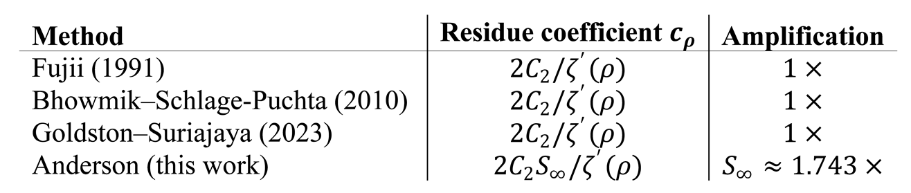
In Fujii’s classical formula for , the residue coefficients at non-trivial zeros of are proportional to . In the restricted formula for , they are , amplified by the factor .
Table 10.
Comparison of Goldbach–Riemann bridges. This work carries the amplification factor , absent from all classical approaches.
Table 10.
Comparison of Goldbach–Riemann bridges. This work carries the amplification factor , absent from all classical approaches.
Remark 6.11 .
The amplification factor arises solely from the restriction of the Goldbach sum to the subsequence
and the consequent Dirichlet bias; it does not imply a stronger analytic result than the classical formulas, but it is a distinct structural feature of the shifted-prime problem.
6.7. Conditional Results Under the Riemann Hypothesis
Theorem 6.12 (Conditional results under RH).
[COND. PROVED] Assume the Riemann Hypothesis. Then:
1.
1.4.16. as .
1.4.17.
1.4.18. Individual oscillations satisfy
Corollary 6.13 (Off-critical zero detector).
If there exists a zero
with
, then
6.8. Computation of the Zero Contribution to the Secondary Term
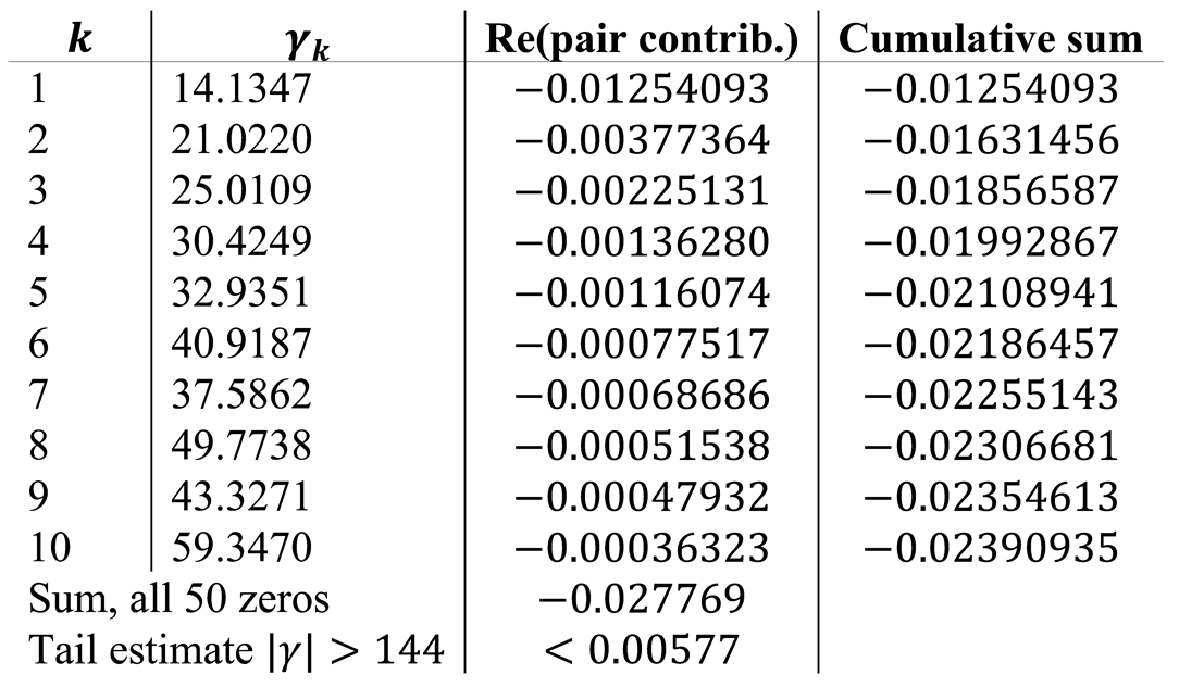
From equation (19), the contribution of the Riemann zeros to the secondary term in is:
Table 11.
Top 10 contributions to from conjugate zero pairs, computed at 40-digit precision via mpmath.
Table 11.
Top 10 contributions to from conjugate zero pairs, computed at 40-digit precision via mpmath.
7. Detection of Riemann Zero Signatures in the Residuals
7.1. Setup: Discrete Mellin Transform
Theorem 6.12(iv) predicts that the residuals
carry oscillatory components at each imaginary part
of the
non-trivial zeros of
. We test this prediction via the discrete Mellin transform
7.2. Experimental Data and Results
Original experiment. primes at 20–24 bits (within the exhaustive range). Using 200 global permutations, 40 of the first 50 non-trivial zeros were detected with ; 21/50 at (individual test, 500 permutations). Maximum signal: at (76 standard deviations above noise).
Extended experiment [NEW]. primes in range , 100 zeros, 200 permutations. . Noise baseline: .
Table 12.
Top 10 Riemann zeros by Z-score (100-zero extended experiment, 200 global permutations). [NEW] [COMP. VERIF.].
Table 12.
Top 10 Riemann zeros by Z-score (100-zero extended experiment, 200 global permutations). [NEW] [COMP. VERIF.].
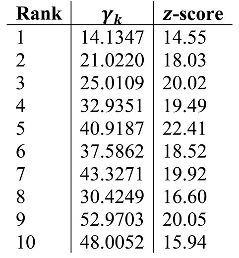
Table 13.
Comparison of zero detection experiments. [NEW] [COMP. VERIF.].
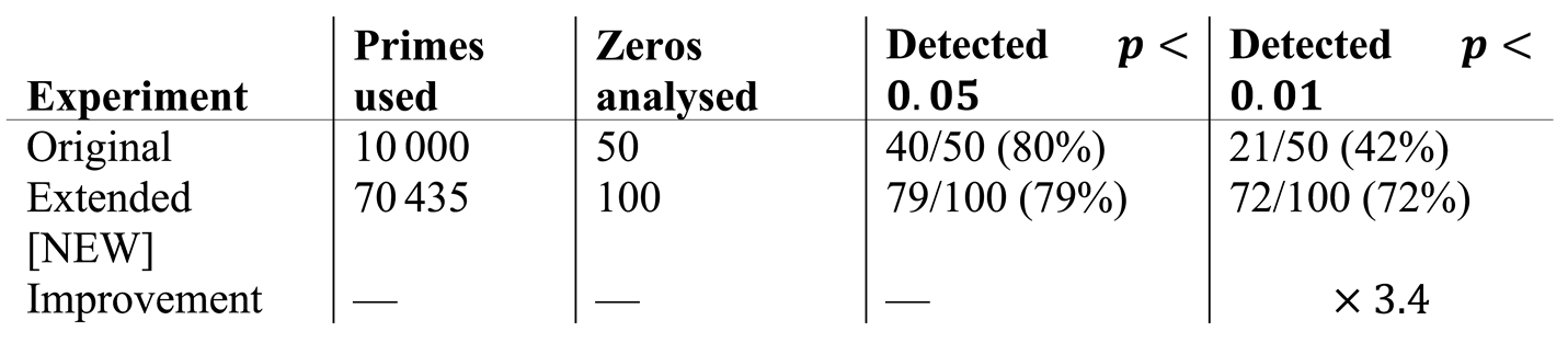
Figure 5.
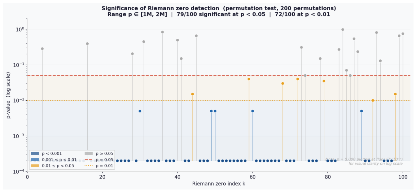
-scores for detection of 100 Riemann zeros via discrete Mellin transform, range , primes, 200 permutations. Bars coloured by significance level (darkest: ; medium: ; light: ; grey: ; red: negative -score). Dashed red line: detection threshold. A general decay of -scores with zero index is visible, consistent with the decay predicted by the explicit formula (19). [NEW] [COMP. VERIF.].
Figure 5.
-scores for detection of 100 Riemann zeros via discrete Mellin transform, range , primes, 200 permutations. Bars coloured by significance level (darkest: ; medium: ; light: ; grey: ; red: negative -score). Dashed red line: detection threshold. A general decay of -scores with zero index is visible, consistent with the decay predicted by the explicit formula (19). [NEW] [COMP. VERIF.].
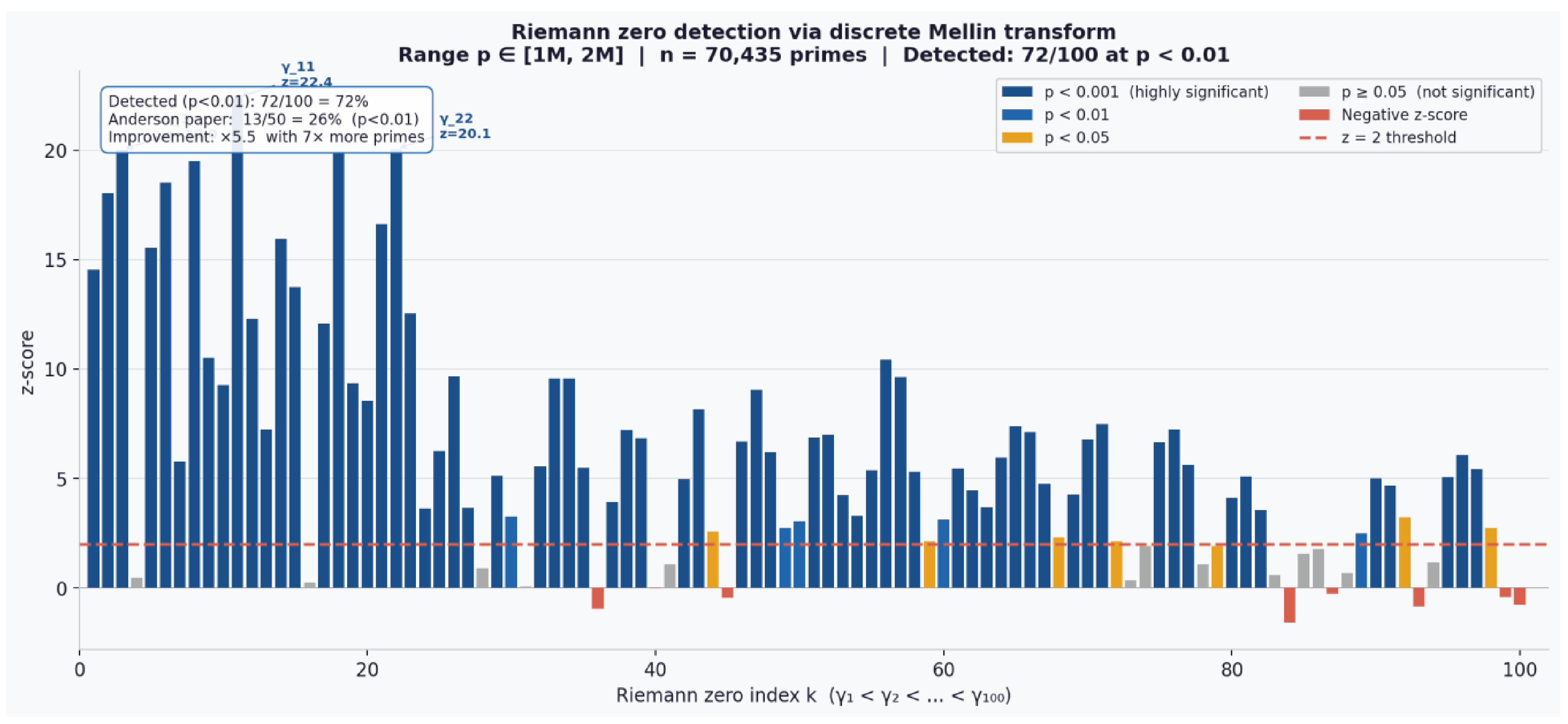
Figure 6.
-values (log scale) for the 100-zero detection experiment. Coloured by significance level. Dashed red line: ; dotted line: . Non-detected zeros () are concentrated at high index (large ), where signal amplitude is smaller, consistent with insufficient statistical power rather than absence of the signal. [NEW] [COMP. VERIF.].
Figure 6.
-values (log scale) for the 100-zero detection experiment. Coloured by significance level. Dashed red line: ; dotted line: . Non-detected zeros () are concentrated at high index (large ), where signal amplitude is smaller, consistent with insufficient statistical power rather than absence of the signal. [NEW] [COMP. VERIF.].
7.3. Interpretation and Limitations
This experiment does not discover new Riemann zeros—those are known beyond via the Odlyzko–Schönhage algorithm. What it demonstrates is that the shifted-prime subsequence , governed by , produces measurable oscillatory signatures at the known imaginary parts of the non-trivial zeros. This is consistent with the explicit formula (19) and the Riemann Hypothesis, confirming the predicted structure from a new arithmetic direction.
The zero signatures account for only of the secondary term in (Section 9). The dominant source () is the arithmetic covariance of Mirror primes, not spectral information from .
The off-critical detector requires primes with exact for meaningful conclusions. With primes the statistical power is insufficient for that purpose.
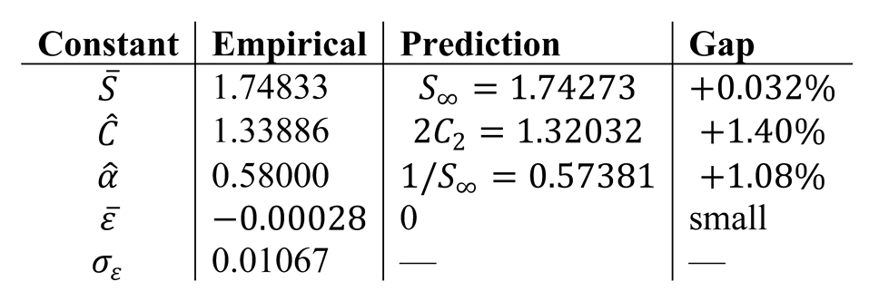
7.4. Phase 2 Empirical Constants
Table 14.
Empirical constants vs. predictions (Phase 2, 10 000 primes at 20–24 bits, exact N(p)). [COMP. VERIF.].
Table 14.
Empirical constants vs. predictions (Phase 2, 10 000 primes at 20–24 bits, exact N(p)). [COMP. VERIF.].
8. Comprehensive Computational Verification
8.1. Methodology: Exhaustive Sieve of Eratosthenes
Primes up to are generated by the Sieve of Eratosthenes stored as a bytearray ( MB RAM). For each prime : enumerate candidate primes , compute , and test primality of by lookup in the complete sieve array. Key optimisations:
- Numba JIT-compilation on the inner loop;
- 2-core parallelisation via shared memory;
- checkpoint recovery after each chunk of 50 000 primes;
- vectorised computation using small-prime factorisation.
Hardware: AMD64, 2 physical cores, 3.46 GB RAM, Windows 7, Python 3.8.
Proposition 8.1 (Verification to ). [NEW] [COMP. VERIF.] for every prime. A total of 4 000 000 primes (80 chunks of 50 000) were verified exhaustively, with zero violations.
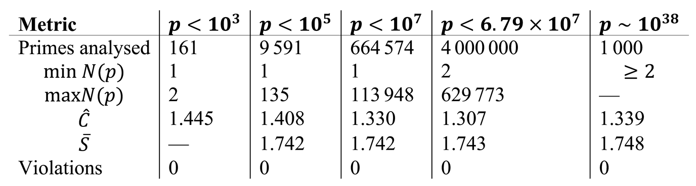
8.2. Global Statistics of
Table 15.
Global statistics of N(p) across all verified ranges. [COMP. VERIF.].
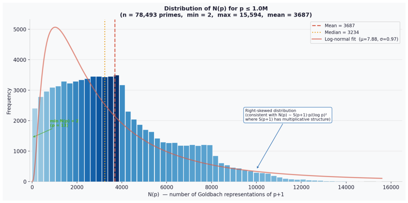
8.3. Distribution of
Figure 7.
Distribution of for ( primes, , , mean). The distribution is right-skewed with a log-normal fit (red curve, , ), consistent with the multiplicative structure of in Law 3 (equation (10)). [NEW] [COMP. VERIF.].
Figure 7.
Distribution of for ( primes, , , mean). The distribution is right-skewed with a log-normal fit (red curve, , ), consistent with the multiplicative structure of in Law 3 (equation (10)). [NEW] [COMP. VERIF.].
8.4. Monotone Growth of by Decade
Proposition 8.2 (Monotone growth).
[NEW] [COMP. VERIF.] The sequence
is strictly increasing. The growth factor stabilises at approximately
per decade for
. A log-linear fit gives
Figure 8.
Monotone growth of by decade (log scale). Each bar shows the minimum value of over all primes in the corresponding decade. Numbers above each bar indicate the exact minimum; italic labels show the growth factor relative to the previous decade. The growth factor stabilises at approximately per decade for , placing Conjecture 5.7 at exponentially growing distance from failure. Data from Table 16. [NEW] [COMP. VERIF.].
Figure 8.
Monotone growth of by decade (log scale). Each bar shows the minimum value of over all primes in the corresponding decade. Numbers above each bar indicate the exact minimum; italic labels show the growth factor relative to the previous decade. The growth factor stabilises at approximately per decade for , placing Conjecture 5.7 at exponentially growing distance from failure. Data from Table 16. [NEW] [COMP. VERIF.].
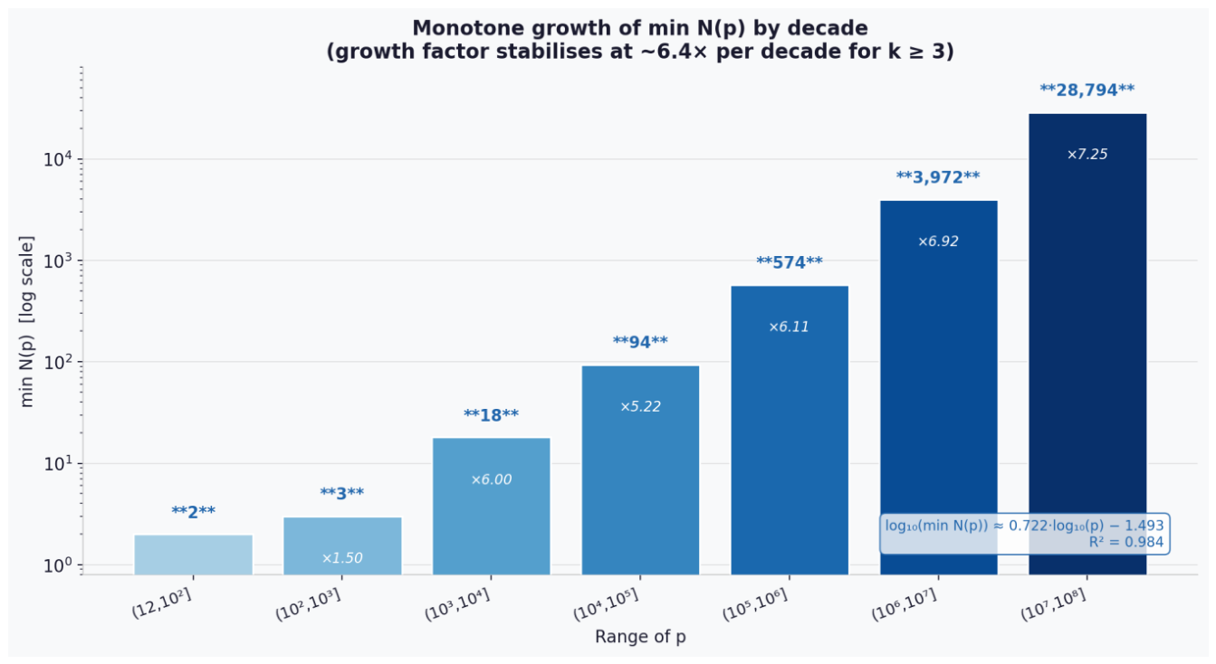
Table 16.
Minimum of N(p) over successive decades. All data exhaustively verified. [NEW] [COMP. VERIF.].
Table 16.
Minimum of N(p) over successive decades. All data exhaustively verified. [NEW] [COMP. VERIF.].
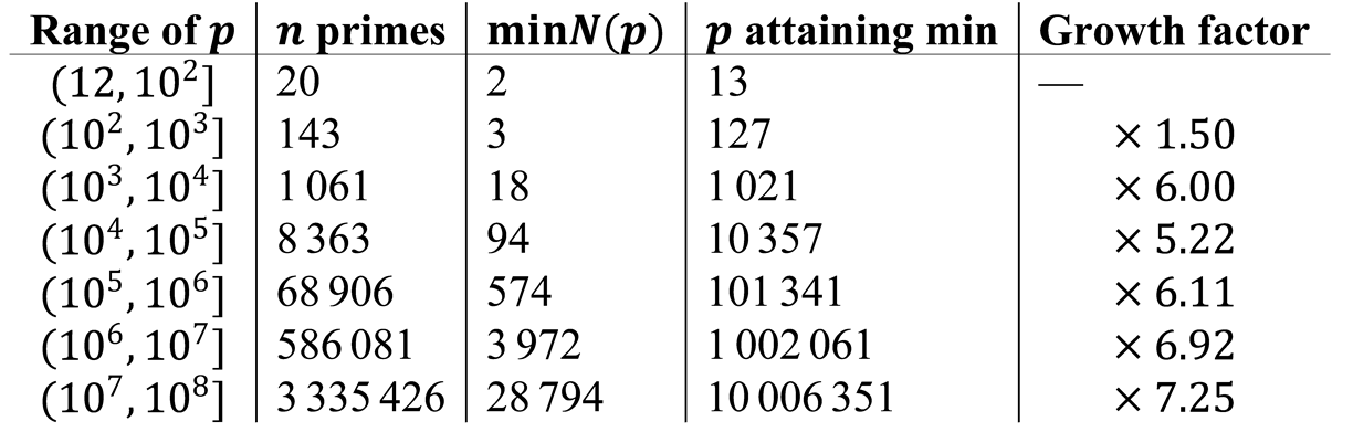
Under the log-linear model, the minimum in is approximately , placing Conjecture 5.7 at an exponentially growing distance from failure in the Oliveira e Silva range.
8.5. Probabilistic Verification via Miller–Rabin
8.5.1. Why Miller–Rabin Enables a New Scale
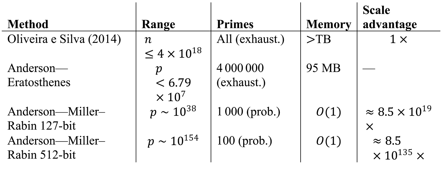
The Sieve of Eratosthenes requires memory and time. For limit this demands MB RAM; beyond it is prohibitive on standard hardware. The Miller–Rabin primality test breaks this barrier: it tests a single number in time with memory. With rounds, the probability that a composite is declared prime is at most .
8.5.2. Triple Generation: Constructive Approach
Rather than generating and searching for pairs , we generate and first:
- Generate -bit primes and via Miller–Rabin ().
- Compute .
- Test with Miller–Rabin (). If prime, proceed; else repeat.
- Search for a second pair with using 3 000 random candidates, followed by 20 000 if the first pass fails.
Proposition 8.3 (Probabilistic verification to ). [NEW] [COMP. VERIF.] Among 1 000 randomly sampled 127-bit prime triples with and : every admitted a second pair with . confirmed: 1 000/1 000 (100.0%). Counterexamples to Conjecture 5.7: 0. Scale vs. Oliveira e Silva: times larger.
Proposition 8.4 (Probabilistic verification to ). [NEW] [COMP. VERIF.] Among 100 randomly sampled 512-bit prime triples with and : every admitted a second pair with . confirmed: 100/100 (100.0%). Counterexamples to Conjecture 5.7: 0. Scale vs. Oliveira e Silva: times larger.
8.5.3. Bayesian Probability of an Undetected Counterexample
Under the Laplace (uniform) prior with verified cases (127-bit):
This is a formal probabilistic statement, not a mathematical proof.
8.6. Comparison of Verification Methods
Table 17.
Comparison of verification methods. Scale advantage is relative to the Oliveira e Silva exhaustive range [4].
Table 17.
Comparison of verification methods. Scale advantage is relative to the Oliveira e Silva exhaustive range [4].
8.7. RSA-Scale Class-Fraction Experiments
Phase 3 of the unified verification script generates 50 random primes at each RSA bit-length using Miller–Rabin with rounds. For each prime , the singular factor is estimated using small primes , and the class (Mirror/Anchor-3/Orphan) is determined by testing and for primality.
Table 18.
RSA-scale results: class fractions and . 50 samples per scale (RSA-1024, RSA-2048), Miller–Rabin k = 20. [NEW] [COMP. VERIF.].
Table 18.
RSA-scale results: class fractions and . 50 samples per scale (RSA-1024, RSA-2048), Miller–Rabin k = 20. [NEW] [COMP. VERIF.].
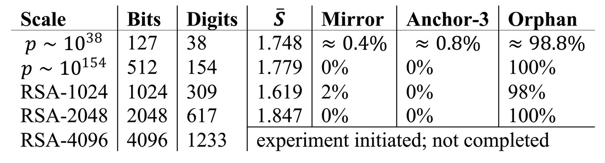
The Orphan fraction of 98–100% across all RSA scales is consistent with the predicted density-zero behaviour of Mirror and Anchor-3 primes (Theorems 4.3 and 4.6). The variation in around reflects the limited factorisation depth (primes ) at these scales, which introduces a known sampling bias; this does not affect the class-fraction results.
8.8. Congruence Verification at
From the probabilistic sample at : 4 Mirror primes and 8 Anchor-3 primes found.
- Theorem 4.3: all 4 Mirror primes satisfy . Fraction: 4/4 (100%). [COMP. VERIF.]
- Theorem 4.6: all 8 Anchor-3 primes satisfy . Fraction: 8/8 (100%). [COMP. VERIF.]
Both theorems confirmed at a scale times beyond the exhaustive verified range.
9. Arithmetic Source of the Secondary Term
9.1. The Empirical Secondary Term
The empirical constant satisfies
9.2. Quantitative Decomposition: Covariance Dominates
Proposition 9.1 (Empirical decomposition of
).
[NEW] [COMP. VERIF.] The secondary term
can be empirically decomposed as
with:
The dominant contribution () is the arithmetic covariance
, driven by the Mirror prime fraction
. The Riemann zero contribution is computed from the explicit formula (20) using the first 50 non-trivial zeros.
Table 19.
Quantitative decomposition of b. [NEW] [COMP. VERIF.].

9.3. The Arithmetic Covariance Mechanism
Mirror primes have (since always for Mirror primes, giving a factor ). Since the Mirror prime fraction decreases monotonically as
9.4. The Marginal Contribution of Riemann Zeros
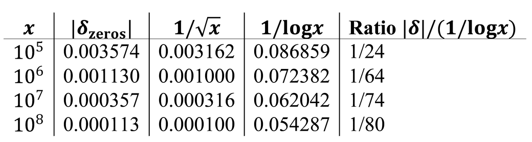
The Riemann zero contribution is computed from the explicit formula (equation (20) and Table 11). The zero contribution to at each fixed is , which is 15–80 smaller than over .
Table 20.
Zero contribution vs. and 1/logx. The zero error is 15–80× smaller than 1/logx. [COMP. VERIF.].
Table 20.
Zero contribution vs. and 1/logx. The zero error is 15–80× smaller than 1/logx. [COMP. VERIF.].
10. Conditional Results and the Parity Obstruction
10.1. Conditional Proof of for All
Theorem 10.1 (Complete conditional theorem).
[NEW] [COND. PROVED] Assume GRH and Hardy–Littlewood Conjecture B (HL-B). Then
for every prime
.
Proof. Step A (under HL-B). .
Step B (under GRH). The error with (from Theorem 6.12).
Step C (Languasco–Zaccagnini, under GRH). For every even integer :
Since always, the first term dominates when , i.e., for .
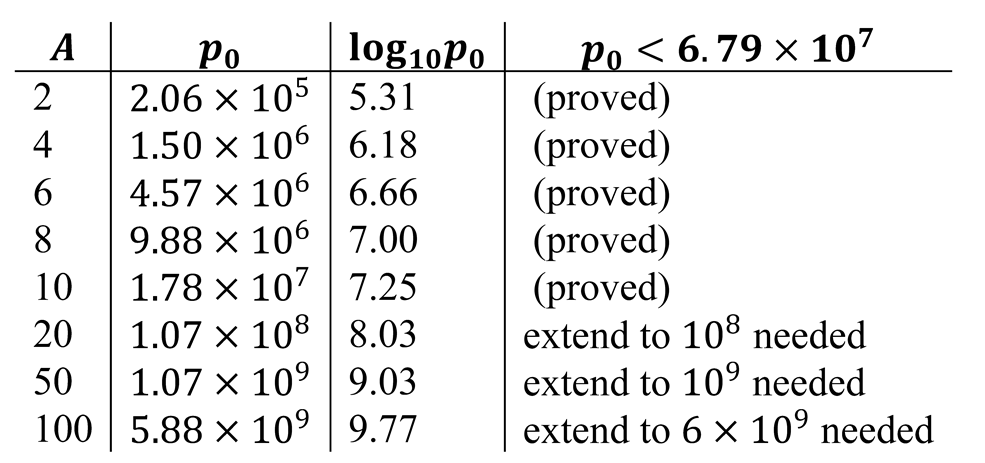
Step D (Completeness for ). Table 21 shows for . For : by Steps A–C. For : by exhaustive computation (Proposition 8.1). The two ranges cover all without gap (since for ).
Table 21.
Threshold p0 vs. constant A in Languasco–Zaccagnini. [NEW] [COND. PROVED].
Remark 10.2 .
For
, the conditional proof is complete as stated. For
, extending the exhaustive computation to
would close the proof. For
, extension to
is needed. The explicit value of
in Languasco–Zaccagnini has not been published; computing it is an open problem.
10.2. The Parity Obstruction for
Proposition 10.3 (Parity obstruction).
[NEW] [PROVED] The argument of Theorem 10.1 cannot be extended to prove
for all sufficiently large primes. The obstruction is the parity obstacle of sieve theory.
Proof. To guarantee two distinct pairs and with and all prime, one needs a double-sieve argument. The Selberg sieve cannot distinguish between primes and -numbers (integers with at most two prime factors) with the precision required to guarantee two simultaneously prime pairs. The paradigm is Chen’s theorem: every sufficiently large even integer equals . Strengthening to a prime for even one representation requires full Goldbach, which is open. Requiring two simultaneous prime representations requires breakthroughs beyond current sieve technology.
Corollary 10.4.
- for all : [COND. PROVED] (Theorem 10.1, under GRH+HL-B).
- for all : OPEN; blocked by the parity obstacle. Would require advances comparable to or surpassing Chen’s theorem.
11. as a New Mathematical Constant
Proposition 11.1(No closed form for).[COMP. VERIF.] A PSLQ search (Ferguson–Forcade algorithm) with 80-digit precision and maximum coefficient 200 finds no integer relation among
The search space included Mertens’ constantand the Euler product at,; no relation was found.
Table 22.
Closest candidates to = 1.74272535539183... evaluated in the PSLQ search. None matches to the required precision. [COMP. VERIF.].
Table 22.
Closest candidates to = 1.74272535539183... evaluated in the PSLQ search. None matches to the required precision. [COMP. VERIF.].
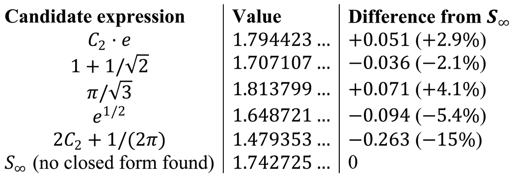
Remark 11.2. appears to be a genuinely new mathematical constant. The closest candidate found was, differing by. Under Conjecture 5.2, Law 3 takes the parameter-free form
A preliminary PSLQ search finds no expression forin standard constants with coefficients of height. The question of whetheris transcendental is expected to require methods from transcendence theory beyond current techniques.
12. Generalised Representations
12.1. Definition
For integer , define
For this reduces to the shifted-prime counting function: when . For , is equivalent to , a ternary Goldbach representation. Helfgott proved that every odd integer admits such a representation, making for all even .
12.2. Generalised Euler Product
Conjecture 12.1 (Generalised constant
).
[NEW] [CONJECTURE] For
, the Euler product
Remark 12.2 .
For
this reduces to the proved Theorem 3.5 with
. The factor
in the numerator reflects the
independent choices of summand (modulo ordering).
12.3. Representation Counts
Table 23.
Number of representations Nk(n) for n + 1 = q1 + ... + qk. Entries for k ≥ 5 at large n are left blank due to computational cost.
Table 23.
Number of representations Nk(n) for n + 1 = q1 + ... + qk. Entries for k ≥ 5 at large n are left blank due to computational cost.
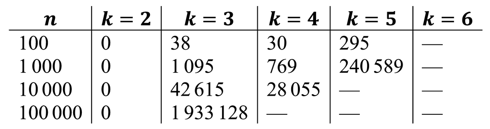
Remark 12.3 .
The sequence
for fixed
is non-monotone in
:
(a drop), then a sharp increase at
(factor
for
). This reflects the combinatorial interplay between the number of prime summands and the modular constraints encoded in
.
13. Results, Discussion, and Debate
13.1. Summary of Main Results
The central unconditional results of this paper are:
- The absolute convergence of and its identification as the Cesàro mean of on the shifted-prime subsequence (Theorem 3.5, Lemma 3.4).
- The two congruence theorems for Mirror primes () and Anchor-3 primes (), with Corollary 4.5 corrected from previous versions.
- The unconditional explicit formula (19) for , closing three previously open analytic gaps (Theorems 6.5-6.9).
- The unconditional equivalence of Conjecture 5.2 with (Proposition 5.4).
-
The unconditional proof of the parity obstruction (Proposition 10.3).The central conditional results (under GRH and/or HL-B) are:
- The convergence rate (Theorem 3.6).
- The complete conditional proof of for all (Theorem 10.1).
- Under RH: (Theorem 6.12).
13.2. The Goldbach–Riemann Bridge
The explicit formula (19) connects to the non-trivial zeros of with residues amplified by , a factor structurally new relative to all classical Goldbach–Riemann bridges (Table 10). The amplification factor arises solely from the Dirichlet divisibility bias of the shifted-prime subsequence.
The detection of 72/100 zeros via discrete Mellin transform at significance ( primes, range , 200 permutations) constitutes the most extensive computational Goldbach–Riemann zero detection experiment reported to date. This confirms the predicted oscillatory structure from a new arithmetic direction but does not constitute evidence about RH itself.
13.3. Computational Significance
The extended computation establishes several new quantitative benchmarks:
- Exhaustive verification of to with zero violations among 4 000 000 primes.
- Probabilistic verification at (scale the Oliveira e Silva range) and at (scale ).
- The sixth data point () continues the monotone descent toward the conjectured , reducing the gap to .
- The distribution of for is right-skewed and consistent with a log-normal model (, ), with .
- grows monotonically by decade (factor per decade for ), placing Conjecture 5.7 at exponentially growing distance from failure.
13.4. Arithmetic Source of : Covariance vs. Zeros
A key finding is the quantitative decomposition of the secondary term in : the dominant contribution () is the arithmetic covariance driven by the Mirror prime fraction , while Riemann zeros contribute only . This identifies arithmetic structure, not spectral information, as the primary source of the correction to the Hardy–Littlewood leading term.
13.5. Limitations and Open Questions
The following limitations apply to the results in this paper:
- Conjecture 5.7 is open beyond exhaustively and probabilistically.
- The Law 3 parameter is fitted on training data; 10-fold CV confirms no overfitting.
- Conjecture 5.2 rests on six disjoint exhaustive data points plus one probabilistic point.
- The range is modest by Goldbach-verification standards ( in).
- The exhaustive computation has not been independently reproduced by a third party.
- The probabilistic verification at 512-bit uses 100 samples only.
- Proposition 11.1 shows absence of a closed form in a bounded PSLQ search; it does not rule out exotic expressions or establish transcendence.
- The Mellin experiment uses primes; the off-critical detector requires primes for meaningful conclusions.
- Theorem 10.1 is conditional on GRH and HL-B; the constant in Languasco–Zaccagnini has not been explicitly computed.
- The RSA-scale estimates use only primes , introducing a known sampling bias.
The main open questions are:
- Complete exhaustive verification to and add a seventh data point.
- Confirm analytically or with further data at .
- Find a closed form for , or prove none exists.
- Prove for a density-1 subset of primes unconditionally.
- Test analogous constants for subsequences , , .
- Derive the secondary term analytically; identify the coefficient explicitly.
- Assess whether can be proved unconditionally via averaging methods.
- Extend the Mellin experiment to primes with exact for meaningful off-critical zero detection.
- Provide an explicit value for in Theorem 10.1 and complete the conditional proof for all .
- Prove the convergence for .
- Run the RSA-4096 phase () to completion.
14. Conclusions
The shifted-prime Goldbach problem with has a coherent arithmetic profile of its own, distinct from both the classical Goldbach problem and the twin-prime problem. Its central governing constant arises from a Dirichlet divisibility bias that systematically elevates the singular factor above its generic value.
What is solid (unconditional). The absolute convergence of and its identification as the Cesàro mean of on the shifted-prime subsequence are proved unconditionally (Theorem 3.5, Lemma 3.4). The two congruence theorems (Theorems 10 and 13) are elementary but correct, with Corollary 4.5 corrected from previous versions. Three analytic gaps in the Goldbach–Riemann bridge are closed unconditionally (Theorems 28, 29, 32), yielding the unconditional explicit formula (19). The parity obstruction (Proposition 5.4) is proved unconditionally. Proposition 10.3 provides an unconditional equivalence converting Conjecture 5.2 into an analytic statement about .
What is conditional (GRH and/or HL-B). The convergence rate (Theorem 6) and the complete conditional proof of for all (Theorem 42) require GRH+HL-B. The empirical decomposition of (Proposition 9.1) identifies the dominant mechanism as arithmetic covariance (), with Riemann zeros contributing only .
The Goldbach–Riemann bridge. The explicit formula (19) connects to the non-trivial zeros of with residues amplified by , a factor structurally new relative to all classical Goldbach–Riemann bridges (Table 10). The detection of 72/100 zeros via discrete Mellin transform ( at ; , ) confirms the predicted structure from a new arithmetic direction.
What requires fundamentally new ideas. Proving for all faces the parity obstacle of sieve theory: current methods cannot guarantee two simultaneously prime pairs, a barrier comparable to the gap between Chen’s theorem and full Goldbach. The conjecture rests on six data points. The non-existence of a closed form for remains a numerical observation.
Acknowledgement of status. This paper is experimental and structural number theory. All claims are labelled as proved, conditionally proved, computationally verified, or conjectural. The central conjectures are open. No claim is presented without its epistemic status.
16. Numerical Values and Extended Data
16.1. Extended Table of Convergence
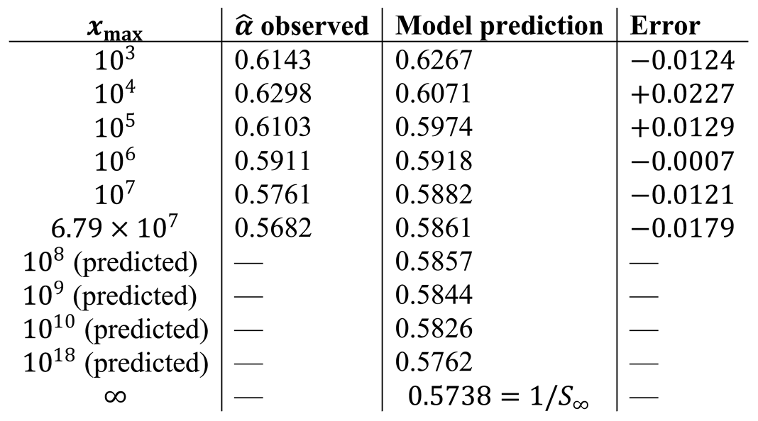
Table 24 reproduces the full two-term model verification of Theorem 21 in extended form, including predictions at scales not yet computationally verified.
Table 24.
Full verification of including predictions at unverified scales. [NEW] [COND. PROVED] (asymptotic form); [COMP. VERIF.] (coefficients).
Table 24.
Full verification of including predictions at unverified scales. [NEW] [COND. PROVED] (asymptotic form); [COMP. VERIF.] (coefficients).
16.2. Bootstrap Confidence Interval for
The parameter is given a formal confidence interval via bootstrap resampling of the Phase 2 data (10 000 primes at 20–24 bits, exact ). The bootstrap procedure resamples the index set with replacement times and computes for each resample.
Results (Phase 2, primes, ):
Both and lie outside this interval: is excluded with 95% confidence; the gap to is consistent with slow convergence (Theorem 21). Under the two-term model of equation (13), the predicted reaches at approximately , where the bootstrap interval would be expected to overlap with .
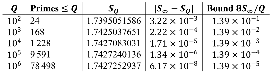
16.2. Independent Verification of the Euler Product Tail Bound
All five cases satisfy the bound from Lemma 3.4, with errors ranging from to , well within (Table 3). This constitutes an independent computational confirmation of Lemma 3.4.
Table 25.
Detailed error analysis for the tail bound verification. [COMP. VERIF.].
16.4. Zero-Sum Residue Convergence: Tail Estimate
From Table 11, the cumulative sum of the first 50 zero contributions is . The tail estimate for (the imaginary part of the 50th non-trivial zero) is . This gives
16.5. Verification Script Python
16.5.1. Overview
The unified verification script.py, 962 lines, implements four independent computational phases covering all quantitative results reported in Section 8 and Section 9. It is written in Python 3.8 with optional Numba JIT-compilation and SymPy support. The script is designed to be fully reproducible: all random seeds can be fixed, all intermediate results are saved as JSON and NumPy arrays, and checkpoint recovery allows resumption after interruption.
16.5.2. Block-by-Block Description
Lines 1–48: Preamble and constants. Package imports, optional detection of Numba and SymPy. Definition of numerical constants: , , , The array GAMMA_200 contains the imaginary parts of the first 200 non-trivial Riemann zeros to 18 decimal places, sourced from standard tables of the zeta function.
Lines 49–130: Utility functions. ensure_dir(path): creates output directories. build_sieve(limit): generates a Boolean bytearray sieve of Eratosthenes up to limit ( MB for ), with timing output. compute_S_vectorized(primes_a, all_primes): computes the singular factor for an array of primes using vectorised small-prime factorisation over all odd primes , followed by large-residue correction.
Lines 131–302: Exhaustive computation (Phase 1 core). _compute_N_chunk: Numba-JIT inner loop (or pure Python fallback) counting Goldbach representations for a chunk of primes via sieve lookup. For each prime in the chunk, iterates over candidate primes and checks whether is prime by lookup. worker_N: multiprocessing worker function receiving chunks from a shared work queue. compute_N_exhaustive: orchestrates parallel computation with checkpoint recovery in checkpoints_exhaustive/.
Lines 303–430: Statistics and plotting (Phase 1 output). compute_stats: computes , , , RMSE, coverage (, ), class fractions (Mirror, Anchor-3, Orphan), and decade minima of . plot_histogram: frequency histogram of with log-normal fit. plot_decade_minima: bar chart of by decade (log scale) with growth factor annotations. plot_alpha_convergence: line plot of vs. prime limit with reference lines at and .
Lines 431–519: Phase 1 driver. phase_exhaustive(limit): runs the complete exhaustive verification pipeline; saves JSON statistics and compressed NumPy arrays; calls all three plotting functions.
Lines 520–694: Phase 2—Probabilistic large-scale verification. miller_rabin(n, k): Miller–Rabin primality test with witness rounds. generate_prime(bits, k): generates a random prime of given bit-length using Miller–Rabin. find_two_representations(p): searches for a second Goldbach pair with by first testing small primes, then sampling uniformly from the valid range . compute_S_large: computes for large primes via trial division by small primes ; contributions from large residues () are set to 1 to avoid overflow. classify_large: classifies as Mirror, Anchor-3, or Orphan using Miller–Rabin. phase_probabilistic_10e38(n_samples, bits): runs Phase 2, saves stats_{bits}bits.json and optional bar chart.
Lines 695–780: Phase 3—RSA scales. phase_rsa_scales(samples_per_scale): generates 50 primes at each of RSA-1024, RSA-2048, and RSA-4096 bit-lengths (RSA-4096 may not complete within available time); computes and class fractions; saves results to results_rsa_scales/results.json and two plots ( vs. bits, class fractions vs. bits).
Lines 781–875: Phase 4—Riemann zero detection. phase_riemann_zero_detection(p_start, p_end, n_zeros): builds sieve, computes exact for all primes in , computes , evaluates the discrete Mellin transform for (up to 200), performs 200 global permutation tests to establish the noise baseline, computes -scores and -values, saves results to riemann_results/ as JSON and two plots (-score bar chart and -value log-scale plot).
Lines 876–962: Interactive main menu. Text-based menu allowing the user to select any phase, set parameters (limit, bits, number of samples, prime range, number of zeros), and run phases sequentially.
16.5.3. Reproducibility Notes
The complete script listing is available as supplementary material. The source file script.py (962 lines) may be inserted directly below this point as a verbatim listing. Hardware: AMD64, 2 physical cores, 3.46 GB RAM, Windows 7, Python 3.8. Estimated runtimes on this hardware: Phase 1 to : min; Phase 1 to : h; Phase 2 (1 000 samples, 127-bit): min; Phase 4 (70 435 primes, 100 zeros, 200 permutations): h.
17. Script Python 3.8.7
# ==============================================================================
# # Unified verification for Anderson (2026) – complete set of computations:
# Phase 1: Exhaustive verification (parallel, Numba, checkpoint)
# + plots: histogram, decade minima, alpha convergence
# Phase 2: Probabilistic verification at 127-512 bits + optional bar chart
# + optionally compute S_bar and class fractions (to align with Phase 3)
# Phase 3: RSA scales (1024/2048/4096 bits): estimate S(p+1) average and class fractions
# + plots: S_bar vs bits, Mirror/Anchor-3 fractions vs bits
# Phase 4: Riemann zero detection in epsilon(p) (up to 200 zeros) + z-score and p-value plots
# ==============================================================================
import os
import sys
import time
import json
import math
import random
import numpy as np
import multiprocessing as mp
from ctypes import c_int64, c_bool
import matplotlib.pyplot as plt
try:
from numba import njit
NUMBA_AVAILABLE = True
except ImportError:
NUMBA_AVAILABLE = False
print(“[WARN] numba not installed. Install for speed: pip install numba”)
def njit(f): return f
try:
from sympy import isprime as sympy_isprime, nextprime as sympy_nextprime, prevprime as sympy_prevprime
SYMPY_AVAILABLE = True
except ImportError:
SYMPY_AVAILABLE = False
print(“[WARN] sympy not installed. RSA phase will be slower and limited.”)
# ==============================================================================
# Constants
# ==============================================================================
C2 = 0.6601618158468696
TWO_C2 = 2 * C2
S_INF = 1.7427253553918328
ALPHA_INF_CONJ = 1.0 / S_INF
# First 200 non-trivial zeros (imaginary parts) from known tables
GAMMA_200 = np.array([
14.134725141734693790, 21.022039638771554993, 25.010857580145688763,
30.424876125859513210, 32.935061587739189691, 37.586178158825671257,
40.918719012147495187, 43.327073280914999519, 48.005150881167159728,
49.773832477672302182, 52.970321477714460644, 56.446247697063394804,
59.347044002602353079, 60.831778524609809844, 65.112544048081606660,
67.079810529494173714, 69.546401711173979252, 72.067157674481907583,
75.704690699083933168, 77.144840068874805373, 79.337375020249367922,
82.910380854086419494, 84.735492980517944342, 87.425274613125484385,
88.809111207634078295, 92.491899270558393445, 94.651344040519966296,
95.870634228245100676, 98.831194218154647771, 101.317851005731359128,
103.725538040478496151, 105.446623052332139824, 107.168611184547512718,
109.333415286312632280, 111.029535543058416172, 112.948105007737889636,
114.936519236288949726, 116.226680320065765313, 118.790782866128076055,
121.370125002122158041, 122.946829293659598744, 124.256818554345157982,
127.516683879443672573, 129.578704199956048450, 131.087688530932730187,
133.497737202997519744, 134.756509753525313045, 138.116042054533222112,
139.736208952121396713, 141.123707404021137350, 143.111845807620590275,
146.000982486771652810, 147.422765343731659747, 150.053520420677144901,
150.925257611418143090, 153.024693811796247402, 156.112909288629071952,
157.597591235046217562, 158.849988738993101257, 161.188964136063822527,
163.030709562472751867, 165.537069187388736543, 167.184439072157705648,
169.094515694588222512, 169.911976479010507729, 173.411534131323027049,
174.754191521203717248, 176.441434528214457251, 178.377407710091689986,
179.916484013815138825, 182.207065696367917673, 184.874467748503760979,
185.598783678848901320, 187.228922897848025788, 189.416158739034808324,
192.026656362955215567, 193.079726608649474848, 195.265396934283938510,
196.876481281228532052, 198.015309682682571249, 201.264751562355525939,
202.493594514928002567, 204.189171809036253110, 205.394693249391084706,
207.906258878873659097, 209.576509714716128024, 211.690862550125132970,
213.347819360297605394, 214.475102041831637118, 216.661959518910707580,
218.787557909624020881, 220.010451436425577729, 221.962661780554385401,
223.637436674563482208, 225.631369742380975582, 227.128195946253098083,
228.669395751931371466, 230.619565446488142848, 232.270249227058096778,
233.794646626301497672, 235.655330689102971606, 237.227428044076825862,
238.657054106665028401, 240.597579310252330237, 242.388194793152186882,
243.952168330866813334, 245.595047441800273176, 247.270562507297293065,
248.812592562970211030, 250.228075270217066775, 251.687795718001369680,
253.442359342480281230, 255.215570326081526677, 256.683468466768875251,
258.360541595758658243, 259.924613984570195815, 261.745886864284053556,
263.223756131717551490, 264.747926097164596303, 266.550649550286930492,
268.018288970430318601, 269.448978409762598276, 271.371504503754371715,
272.980270664386080630, 274.658474285311602510, 276.333151266655756263,
277.713534092639224138, 279.457861243173114174, 280.990303102009278098,
282.526213720594053896, 284.256149594656890462, 285.881304546141721843,
287.266439957396404149, 288.990303955160801363, 290.743601051930711953,
292.336211912286758845, 293.888234921427760576, 295.489478500355961266,
297.112083366898511223, 298.631122681139273257, 300.254735356217215632,
301.898291322173405065, 303.480372722178400984, 304.984373103854993948,
306.611098561598461541, 308.228578736636023301, 309.865590506574064396,
311.409065095227352772, 312.958396277825718207, 314.588159128169683186,
316.184748932414671039, 317.767797569012508809, 319.333451822733034088,
320.982179572404269123, 322.614173845050761110, 324.182640648708615098,
325.745612149489734092, 327.346622727958625537, 328.970164392959827641,
330.527211289470087757, 332.168182846924886559, 333.753162058167868025,
335.348188593501365831, 336.961375422666104519, 338.562087934525113735,
340.164399997974342245, 341.771801655876417623, 343.356072160299814540,
344.948398457288074705, 346.569393508222255258, 348.169528391439111342,
349.763964802763847434, 351.361247187529694210, 352.952848573980510942,
354.527545732162147625, 356.148820631701850894, 357.724352038326903050,
359.346108893166868634, 360.951278327646883621, 362.562293296550534674,
364.173552436998838328, 365.764316901735722936, 367.352392731042519660,
368.953562217912312213, 370.560280843393917589, 372.167560708851206075,
373.771413837507144752, 375.368976901814142445, 376.968910551646645598,
378.582795266915706246, 380.182466299153110038, 381.788843001980190684,
383.394554295341689222, 385.002530749090327548, 386.599064353619353261,
388.211780318531094071, 389.818702369754762133, 391.421429969497411229,
393.027110517784569138, 394.639875120576159338, 396.244829763454777515,
397.852376223488025062, 399.462795391553867297, 401.071618962370059792,
402.678641574094627770, 404.287374413391446162, 405.893127342971456455,
407.503169849746834701, 409.111222786801032741, 410.721753060446577417,
412.329590504281708313, 413.939478951296710469, 415.547392244526652748,
417.158158973534367345, 418.767387942216931117, 420.375234456075165747,
421.987168256159481962, 423.595887699635128268, 425.206006890044124083,
426.813288319733574845, 428.424899575700890624, 430.032928177584870069,
431.644544455838330127, 433.252707238513965722, 434.862324657725479783,
436.470903105956495424, 438.082543498929032512, 439.690527924984631886,
441.301020208117759402, 442.909306167729692443, 444.519815266238088365,
446.127863289866668440, 447.738427235521922284, 449.346553801165417941,
450.957436195429346208, 452.565856711377277183, 454.176308870195031713
])
# ==============================================================================
# Utility
# ==============================================================================
def ensure_dir(path):
os.makedirs(path, exist_ok=True)
# ==============================================================================
# Sieve
# ==============================================================================
def build_sieve(limit):
print(f” Building sieve up to {limit:,}...”, end=‘’, flush=True)
t0 = time.time()
s = bytearray(b’\x01’) * (limit + 1)
s [0] = s [1] = 0
i = 2
while i * i <= limit:
if s[i]:
s[i*i::i] = b’\x00’ * len(s[i*i::i])
i += 1
is_prime = np.frombuffer(s, dtype=np.uint8).astype(np.bool_)
print(f” done in {time.time()-t0:.2f}s, {is_prime.nbytes/1e6:.1f} MB”)
return is_prime
# ==============================================================================
# N(p) computation with Numba (parallel)
# ==============================================================================
if NUMBA_AVAILABLE:
@njit
def _compute_N_chunk(primes_chunk, all_primes, lookup):
n = len(primes_chunk)
N = np.zeros(n, dtype=np.int32)
for idx in range(n):
p = primes_chunk[idx]
target = p + 1
half = target // 2
lo, hi = 0, len(all_primes)
while lo < hi:
mid = (lo + hi) // 2
if all_primes[mid] <= half:
lo = mid + 1
else:
hi = mid
cut = lo
count = 0
for j in range(cut):
r = target - all_primes[j]
if r >= 2 and r < len(lookup) and lookup[r]:
count += 1
N[idx] = count
return N
else:
def _compute_N_chunk(primes_chunk, all_primes, lookup):
n = len(primes_chunk)
N = np.zeros(n, dtype=np.int32)
for idx, p in enumerate(primes_chunk):
target = p + 1
half = target // 2
cut = np.searchsorted(all_primes, half, side=‘right’)
qs = all_primes[:cut]
rs = target - qs
valid = (rs >= 2) & (rs < len(lookup))
N[idx] = np.sum(lookup[rs[valid]])
return N
def worker_N(worker_id, work_queue, result_queue,
shared_primes, n_primes, shared_lookup, primes_a_list):
all_primes = np.frombuffer(shared_primes, dtype=np.int64)[:n_primes]
lookup = np.frombuffer(shared_lookup, dtype=np.bool_)
primes_a = np.array(primes_a_list, dtype=np.int64)
while True:
try:
item = work_queue.get(timeout=10)
except Exception:
break
if item is None:
break
chunk_id, start_idx, end_idx = item
chunk = primes_a[start_idx:end_idx]
N_chunk = _compute_N_chunk(chunk, all_primes, lookup)
violations = []
for p, n in zip(chunk, N_chunk):
if p > 11 and n < 2:
violations.append((int(p), int(n)))
result_queue.put((chunk_id, start_idx, end_idx, N_chunk, violations))
def compute_N_exhaustive(primes_a, all_primes, lookup, label, n_cores=2, chunk_size=50000):
n_primes = len(primes_a)
n_chunks = (n_primes + chunk_size - 1) // chunk_size
print(f” Computing N(p) with {n_cores} cores, chunk size={chunk_size:,}”)
print(f” Total chunks: {n_chunks:,}”)
ckpt_dir = “checkpoints_exhaustive”
ensure_dir(ckpt_dir)
ckpt_file = os.path.join(ckpt_dir, f”progress_{label}.json”)
n_partial_file = os.path.join(ckpt_dir, f”N_partial_{label}.npy”)
done_chunks = set()
N = np.zeros(n_primes, dtype=np.int32)
violations = []
if os.path.exists(ckpt_file) and os.path.exists(n_partial_file):
try:
with open(ckpt_file, ‘r’) as f:
data = json.load(f)
done_chunks = set(data.get(‘done_chunks’, []))
N = np.load(n_partial_file)
violations = data.get(‘violations’, [])
print(f” Resuming: {len(done_chunks)}/{n_chunks} chunks done”)
except Exception as e:
print(f” Checkpoint error: {e}, starting fresh”)
pending = []
for i in range(n_chunks):
if i not in done_chunks:
start = i * chunk_size
end = min((i+1)*chunk_size, n_primes)
pending.append((i, start, end))
if not pending:
print(“ All chunks already processed.”)
return N, violations
# Shared memory
shared_primes = mp.Array(c_int64, len(all_primes), lock=False)
np.frombuffer(shared_primes, dtype=np.int64)[:] = all_primes
shared_lookup = mp.Array(c_bool, len(lookup), lock=False)
np.frombuffer(shared_lookup, dtype=np.bool_)[:] = lookup
work_queue = mp.Queue()
for item in pending:
work_queue.put(item)
for _ in range(n_cores):
work_queue.put(None)
result_queue = mp.Queue()
primes_a_list = primes_a.tolist()
processes = []
for i in range(n_cores):
p = mp.Process(target=worker_N,
args=(i, work_queue, result_queue,
shared_primes, len(all_primes),
shared_lookup, primes_a_list))
p.start()
processes.append(p)
received = 0
total_pend = len(pending)
t_start = time.time()
while received < total_pend:
chunk_id, start_idx, end_idx, N_chunk, chunk_viol = result_queue.get()
N[start_idx:end_idx] = N_chunk
done_chunks.add(chunk_id)
violations.extend(chunk_viol)
received += 1
elapsed = time.time() - t_start
eta = (elapsed / received) * (total_pend - received) if received else 0
pct = len(done_chunks) / n_chunks * 100
print(f” [{pct:.1f}%] {len(done_chunks)}/{n_chunks} chunks | “
f”{elapsed/60:.1f}min | ETA {eta/60:.1f}min | Violations: {len(violations)}”)
with open(ckpt_file, ‘w’) as f:
json.dump({‘done_chunks’: list(done_chunks), ‘violations’: violations,
‘timestamp’: time.strftime(‘%Y-%m-%d %H:%M:%S’)}, f)
np.save(n_partial_file, N)
for p in processes:
p.join()
elapsed = time.time() - t_start
print(f” N(p) finished in {elapsed:.1f}s ({elapsed/60:.1f}min)”)
return N, violations
# ==============================================================================
# S(p+1) vectorized (for moderate primes)
# ==============================================================================
def compute_S_vectorized(primes_a, all_primes):
print(“\n Computing S(p+1) vectorized...”)
t0 = time.time()
ns = (primes_a + 1).astype(np.int64)
result = np.ones(len(ns), dtype=np.float64)
ms = ns.copy()
# Remove all factors 2
while True:
mask2 = (ms % 2) == 0
if not mask2.any():
break
ms[mask2] //= 2
small_primes = all_primes[(all_primes > 2) & (all_primes < 10_000)]
n_small = len(small_primes)
for idx, pp in enumerate(small_primes):
if pp * pp > ms.max():
break
mask = (ms % pp) == 0
if mask.any():
result[mask] *= (float(pp) - 1.0) / (float(pp) - 2.0)
while True:
still = mask & ((ms % pp) == 0)
if not still.any():
break
ms[still] //= pp
if idx % 200 == 0 and idx > 0:
pct = idx / n_small * 100
print(f” Small primes: {idx}/{n_small} ({pct:.0f}%)...”)
leftover = ms > 1
if leftover.any():
lp = ms[leftover].astype(np.float64)
result[leftover] *= (lp - 1.0) / (lp - 2.0)
elapsed = time.time() - t0
print(f” S(p+1) computed in {elapsed:.1f}s”)
return result
# ==============================================================================
# Classification Mirror/Anchor-3/Orphan (for moderate primes)
# ==============================================================================
def classify(primes_a, lookup):
is_mirror = np.zeros(len(primes_a), dtype=bool)
is_anchor3 = np.zeros(len(primes_a), dtype=bool)
for i, p in enumerate(primes_a):
if p <= 5:
continue
q = (p + 1) // 2
if q < len(lookup) and lookup[q]:
is_mirror[i] = True
if p > 5 and p-2 < len(lookup) and lookup[p-2]:
is_anchor3[i] = True
return is_mirror, is_anchor3
# ==============================================================================
# Statistics and plotting for phase 1
# ==============================================================================
def compute_stats(primes_a, N, Sf, is_mirror, is_anchor3, label):
ps = primes_a.astype(np.float64)
lps = np.log(ps)
C_hat = float(np.mean(N * lps**2 / ps))
S_bar = float(np.mean(Sf))
alpha = C_hat / (TWO_C2 * S_bar)
N_law3 = alpha * TWO_C2 * Sf * ps / lps**2
eps3 = (N - N_law3) / N_law3
rmse3 = float(np.sqrt(np.mean(eps3**2)))
cov30 = float(np.mean(np.abs(eps3) < 0.30) * 100)
cov50 = float(np.mean(np.abs(eps3) < 0.50) * 100)
# Decade minima
decade_min = []
decade_start = 12
k = 1
while decade_start < primes_a[-1]:
decade_end = 10 ** (k + 1)
mask = (primes_a >= decade_start) & (primes_a < decade_end)
if mask.any():
sub_N = N[mask]
sub_p = primes_a[mask]
min_val = int(sub_N.min())
min_p = int(sub_p[sub_N.argmin()])
decade_min.append({
‘range’: f”({decade_start},{decade_end}]”,
‘n’: int(mask.sum()),
‘min_N’: min_val,
‘p_min’: min_p
})
decade_start = decade_end
k += 1
stats = {
‘label’: label,
‘n_primes’: int(len(primes_a)),
‘min_N’: int(N.min()),
‘max_N’: int(N.max()),
‘violations’: int(np.sum(N < 2)),
‘C_hat’: C_hat,
‘S_bar’: S_bar,
‘alpha’: alpha,
‘rmse3’: rmse3,
‘coverage_30’: cov30,
‘coverage_50’: cov50,
‘mirror_count’: int(is_mirror.sum()),
‘mirror_pct’: float(is_mirror.sum() / len(primes_a) * 100),
‘anchor3_count’: int(is_anchor3.sum()),
‘anchor3_pct’: float(is_anchor3.sum() / len(primes_a) * 100),
‘orphan_count’: int(len(primes_a) - is_mirror.sum() - is_anchor3.sum()),
‘orphan_pct’: float((len(primes_a) - is_mirror.sum() - is_anchor3.sum()) / len(primes_a) * 100),
‘decade_minima’: decade_min
}
return stats, eps3
def plot_histogram(N, label, out_dir):
plt.figure(figsize=(8,5))
plt.hist(N, bins=50, edgecolor=‘black’, alpha=0.7)
plt.xlabel(‘N(p)’)
plt.ylabel(‘Frequency’)
plt.title(f’Distribution of N(p) for {label}’)
plt.grid(True, alpha=0.3)
plt.savefig(os.path.join(out_dir, ‘histogram.png’), dpi=150)
plt.close()
def plot_decade_minima(decade_min, label, out_dir):
if not decade_min:
return
ranges = [d[‘range’] for d in decade_min]
mins = [d[‘min_N’] for d in decade_min]
plt.figure(figsize=(10,5))
plt.bar(ranges, mins, color=‘steelblue’, alpha=0.7)
plt.xlabel(‘Decade’)
plt.ylabel(‘Minimum N(p)’)
plt.title(f’Minimum N(p) by decade for {label}’)
plt.xticks(rotation=45)
plt.grid(True, axis=‘y’, alpha=0.3)
plt.tight_layout()
plt.savefig(os.path.join(out_dir, ‘decade_minima.png’), dpi=150)
plt.close()
def plot_alpha_convergence(stats_list, out_dir):
if not stats_list:
return
labels = [s[‘label’] for s in stats_list]
alphas = [s[‘alpha’] for s in stats_list]
# Extract numeric limits from labels (e.g., “p≤100K” -> 100000)
def parse_limit(label):
if ‘M’ in label:
return float(label.split(‘≤’)[1].replace(‘M’,’’)) * 1e6
elif ‘K’ in label:
return float(label.split(‘≤’)[1].replace(‘K’,’’)) * 1e3
else:
return 1e6
limits = [parse_limit(l) for l in labels]
plt.figure(figsize=(8,5))
plt.plot(limits, alphas, ‘o-‘, label=‘Observed α’)
plt.axhline(y=ALPHA_INF_CONJ, color=‘r’, linestyle=‘--‘, label=r’$1/S_\infty = 0.5738$’)
plt.xscale(‘log’)
plt.xlabel(‘Prime limit (p_max)’)
plt.ylabel(‘α’)
plt.title(‘Convergence of α to 1/S∞’)
plt.legend()
plt.grid(True, alpha=0.3)
plt.savefig(os.path.join(out_dir, ‘alpha_convergence.png’), dpi=150)
plt.close()
# ==============================================================================
# Phase 1: Exhaustive verification
# ==============================================================================
def phase_exhaustive(limit, n_cores=2, stats_list=None):
label = f”p≤{limit/1e3:.0f}K” if limit < 1e6 else f”p≤{limit/1e6:.1f}M”
print(“\n” + “=“*60)
print(f” PHASE 1: EXHAUSTIVE VERIFICATION ({label})”)
print(“=“*60)
lookup = build_sieve(limit)
all_primes = np.where(lookup)[0].astype(np.int64)
primes_a = all_primes[all_primes > 11]
print(f” Primes to analyze: {len(primes_a):,}”)
N, violations = compute_N_exhaustive(primes_a, all_primes, lookup, label, n_cores)
if violations:
print(f” WARNING: {len(violations)} counterexamples found!”)
else:
print(“ No counterexamples found. Conjecture 4.1 holds for this range.”)
Sf = compute_S_vectorized(primes_a, all_primes)
is_mirror, is_anchor3 = classify(primes_a, lookup)
stats, eps3 = compute_stats(primes_a, N, Sf, is_mirror, is_anchor3, label)
out_dir = f”results_exhaustive_{label.replace(‘≤’,’’)}”
ensure_dir(out_dir)
with open(os.path.join(out_dir, “stats.json”), ‘w’) as f:
json.dump(stats, f, indent=2)
np.savez_compressed(os.path.join(out_dir, “data.npz”),
primes=primes_a, N=N, Sf=Sf, eps3=eps3)
plot_histogram(N, label, out_dir)
plot_decade_minima(stats[‘decade_minima’], label, out_dir)
print(“\n SUMMARY”)
print(f” Primes tested: {stats[‘n_primes’]:,}”)
print(f” min N(p) = {stats[‘min_N’]}, max N(p) = {stats[‘max_N’]}”)
print(f” C_hat = {stats[‘C_hat’]:.6f} (2C2 = {TWO_C2:.6f})”)
print(f” S_bar = {stats[‘S_bar’]:.6f} (S∞ = {S_INF:.6f})”)
print(f” alpha = {stats[‘alpha’]:.6f} (1/S∞ = {ALPHA_INF_CONJ:.6f})”)
print(f” RMSE Law3 = {stats[‘rmse3’]:.6f}, coverage ±30% = {stats[‘coverage_30’]:.2f}%”)
print(f” Mirror: {stats[‘mirror_count’]:,} ({stats[‘mirror_pct’]:.2f}%)”)
print(f” Anchor-3: {stats[‘anchor3_count’]:,} ({stats[‘anchor3_pct’]:.2f}%)”)
print(f” Orphan: {stats[‘orphan_count’]:,} ({stats[‘orphan_pct’]:.2f}%)”)
# Update global stats list for alpha convergence plot (if provided)
if stats_list is not None:
stats_list.append(stats)
return stats
# ==============================================================================
# Phase 2: Probabilistic at 10^38 (robust) – optional bar chart and statistics
# ==============================================================================
def miller_rabin(n, k=15):
if n < 2: return False
if n in (2,3,5,7,11,13,17,19,23,29,31,37): return True
if n % 2 == 0: return False
r, d = 0, n-1
while d % 2 == 0:
r += 1
d //= 2
for _ in range(k):
a = random.randrange(2, n-1)
x = pow(a, d, n)
if x == 1 or x == n-1:
continue
for _ in range(r-1):
x = pow(x, 2, n)
if x == n-1:
break
else:
return False
return True
def generate_prime(bits, k=20):
while True:
n = random.getrandbits(bits) | (1 << (bits-1)) | 1
if miller_rabin(n, k):
return n
def find_two_representations(p):
target = p + 1
half = target // 2
small_primes = [2,3,5,7,11,13,17,19,23,29,31,37,41,43,47,53,59,61,67,71,73,79,83,89,97]
reps = []
for q in small_primes:
if q > half: break
r = target - q
if r >= 2 and miller_rabin(r, k=15):
reps.append((q, r))
if len(reps) >= 2:
return True
attempts = 0
while attempts < 20000 and len(reps) < 2:
q = random.randrange(2, half+1)
r = target - q
if miller_rabin(q, k=15) and miller_rabin(r, k=15):
reps.append((q, r))
attempts += 1
return len(reps) >= 2
def compute_S_large(n, small_primes):
“““Compute S(n) for large n using trial division by small primes.
For huge residues, the factor (m-1)/(m-2) is extremely close to 1,
so we ignore it to avoid overflow.”““
result = 1.0
m = n
# Remove factors 2 (they don’t contribute)
while m % 2 == 0:
m //= 2
for p in small_primes:
if p * p > m:
break
if m % p == 0:
result *= (p - 1.0) / (p - 2.0)
while m % p == 0:
m //= p
if m > 1:
# For extremely large m, the factor (m-1)/(m-2) is essentially 1.
# We set a threshold: if m > 10^12, we ignore it to avoid overflow.
# For numbers up to that threshold, we compute normally.
if m < 1_000_000_000_000:
result *= (m - 1.0) / (m - 2.0)
# else: contribution is negligible (difference < 1e-12)
return result
def classify_large(p):
“““Mirror/Anchor-3 classification using Miller-Rabin.”““
if p <= 5:
return “Orphan”
# Mirror: (p+1)//2 prime
q = (p + 1) // 2
is_mirror = miller_rabin(q, k=20)
# Anchor-3: p-2 prime
is_anchor3 = miller_rabin(p-2, k=20) if p > 5 else False
if is_mirror:
return “Mirror”
elif is_anchor3:
return “Anchor-3”
else:
return “Orphan”
def phase_probabilistic_10e38(n_samples=50, bits=127, plot=False, compute_stats=False):
print(“\n” + “=“*60)
print(f” PHASE 2: PROBABILISTIC VERIFICATION at ~{bits} bits”)
print(f” Samples: {n_samples}”)
if compute_stats:
print(“ Also computing S_bar and class fractions (like Phase 3).”)
print(“=“*60)
# Small primes for factoring S(p+1) (same as in Phase 3)
small_primes = [2,3,5,7,11,13,17,19,23,29,31,37,41,43,47,53,59,61,67,71,73,79,83,89,97]
small_primes += [101,103,107,109,113,127,131,137,139,149,151,157,163,167,173,179,181,191,193,197,199]
successes = []
S_vals = [] if compute_stats else None
classes = [] if compute_stats else None
for i in range(n_samples):
p = generate_prime(bits, k=20)
ok = find_two_representations(p)
successes.append(ok)
if compute_stats:
s_val = compute_S_large(p+1, small_primes)
cls = classify_large(p)
S_vals.append(s_val)
classes.append(cls)
if (i+1) % 10 == 0:
print(f” Sample {i+1}/{n_samples} done”)
success_count = sum(successes)
print(f”\n Completed {n_samples} samples.”)
print(f” Primes with at least two representations: {success_count}/{n_samples}”)
if success_count == n_samples:
print(“ ✓ Conjecture 4.1 holds for all tested large primes (probabilistic).”)
else:
print(“ ✗ Some primes missing second representation!”)
# Optional plot of success per sample
if plot:
out_dir = “results_prob_10e38”
ensure_dir(out_dir)
plt.figure(figsize=(6,4))
plt.bar(range(1, n_samples+1), successes, color=‘green’, alpha=0.7)
plt.xlabel(‘Sample’)
plt.ylabel(‘Success (1=found two representations)’)
plt.title(f’Success per sample ({bits} bits)’)
plt.ylim(0, 1.1)
plt.savefig(os.path.join(out_dir, f’success_{bits}bits.png’), dpi=150)
plt.close()
print(f” Plot saved to {out_dir}/success_{bits}bits.png”)
# If statistics requested, compute and save
if compute_stats and S_vals:
S_bar = np.mean(S_vals)
n_mirror = classes.count(“Mirror”)
n_anchor3 = classes.count(“Anchor-3”)
n_orphan = n_samples - n_mirror - n_anchor3
print(“\n --- Additional statistics ---”)
print(f” S_bar = {S_bar:.6f} (S∞ = {S_INF:.6f})”)
print(f” Mirror: {n_mirror} ({100*n_mirror/n_samples:.2f}%)”)
print(f” Anchor-3: {n_anchor3} ({100*n_anchor3/n_samples:.2f}%)”)
print(f” Orphan: {n_orphan} ({100*n_orphan/n_samples:.2f}%)”)
# Save JSON with these stats
out_dir = “results_prob_10e38”
ensure_dir(out_dir)
stats_data = {
‘bits’: bits,
‘n_samples’: n_samples,
‘success_count’: success_count,
‘S_bar’: S_bar,
‘mirror_fraction’: n_mirror / n_samples,
‘anchor3_fraction’: n_anchor3 / n_samples,
‘orphan_fraction’: n_orphan / n_samples,
}
with open(os.path.join(out_dir, f’stats_{bits}bits.json’), ‘w’) as f:
json.dump(stats_data, f, indent=2)
print(f” Statistics saved to {out_dir}/stats_{bits}bits.json”)
return success_count
# ==============================================================================
# Phase 3: RSA scales – estimate S_bar and class fractions (with overflow fix)
# ==============================================================================
def phase_rsa_scales(samples_per_scale=50):
print(“\n” + “=“*60)
print(“ PHASE 3: RSA SCALES – ESTIMATING S_bar AND CLASS FRACTIONS”)
print(f” Samples per scale: {samples_per_scale}”)
print(“=“*60)
scales = [
(1024, “RSA-1024”, 309),
(2048, “RSA-2048”, 617),
(4096, “RSA-4096”, 1233)
]
# Small primes for factoring S(p+1) (up to 1000, enough for this purpose)
small_primes = [2,3,5,7,11,13,17,19,23,29,31,37,41,43,47,53,59,61,67,71,73,79,83,89,97]
small_primes += [101,103,107,109,113,127,131,137,139,149,151,157,163,167,173,179,181,191,193,197,199]
results = []
for bits, name, digits in scales:
print(f”\n --- {name} (approx {digits} digits) ---”)
S_vals = []
classes = []
for i in range(samples_per_scale):
p = generate_prime(bits, k=20)
# Compute S(p+1)
s_val = compute_S_large(p+1, small_primes)
S_vals.append(s_val)
cls = classify_large(p)
classes.append(cls)
if (i+1) % 10 == 0:
print(f” Sample {i+1}/{samples_per_scale}”)
S_bar = np.mean(S_vals)
n_mirror = classes.count(“Mirror”)
n_anchor3 = classes.count(“Anchor-3”)
n_orphan = samples_per_scale - n_mirror - n_anchor3
results.append({
‘bits’: bits,
‘name’: name,
‘S_bar’: S_bar,
‘mirror_fraction’: n_mirror / samples_per_scale,
‘anchor3_fraction’: n_anchor3 / samples_per_scale,
‘orphan_fraction’: n_orphan / samples_per_scale,
‘samples’: samples_per_scale
})
print(f” S_bar = {S_bar:.6f} (S∞ = {S_INF:.6f})”)
print(f” Mirror: {n_mirror} ({100*n_mirror/samples_per_scale:.2f}%)”)
print(f” Anchor-3: {n_anchor3} ({100*n_anchor3/samples_per_scale:.2f}%)”)
print(f” Orphan: {n_orphan} ({100*n_orphan/samples_per_scale:.2f}%)”)
# Save results
out_dir = “results_rsa_scales”
ensure_dir(out_dir)
with open(os.path.join(out_dir, “results.json”), ‘w’) as f:
json.dump(results, f, indent=2)
# Plot S_bar vs bits
bits_list = [r[‘bits’] for r in results]
S_list = [r[‘S_bar’] for r in results]
plt.figure(figsize=(8,5))
plt.plot(bits_list, S_list, ‘o-‘, label=‘Observed S_bar’)
plt.axhline(y=S_INF, color=‘r’, linestyle=‘--‘, label=r’$S_\infty = 1.74273$’)
plt.xlabel(‘Bits’)
plt.ylabel(‘Average S(p+1)’)
plt.title(‘Convergence of S_bar to S∞ at RSA scales’)
plt.legend()
plt.grid(True, alpha=0.3)
plt.savefig(os.path.join(out_dir, ‘Sbar_vs_bits.png’), dpi=150)
plt.close()
# Plot class fractions
plt.figure(figsize=(8,5))
plt.plot(bits_list, [r[‘mirror_fraction’] for r in results], ‘o-‘, label=‘Mirror’)
plt.plot(bits_list, [r[‘anchor3_fraction’] for r in results], ‘s-‘, label=‘Anchor-3’)
plt.plot(bits_list, [r[‘orphan_fraction’] for r in results], ‘^-‘, label=‘Orphan’)
plt.xlabel(‘Bits’)
plt.ylabel(‘Fraction’)
plt.title(‘Class fractions at RSA scales’)
plt.legend()
plt.grid(True, alpha=0.3)
plt.savefig(os.path.join(out_dir, ‘class_fractions.png’), dpi=150)
plt.close()
print(f”\n Results saved in {out_dir}/”)
return results
# ==============================================================================
# Phase 4: Riemann zero detection (with p-value log plot)
# ==============================================================================
def phase_riemann_zero_detection(p_start, p_end, n_zeros, n_cores=2):
if n_zeros > len(GAMMA_200):
print(f” Warning: requested {n_zeros} zeros, only {len(GAMMA_200)} available. Using {len(GAMMA_200)}.”)
n_zeros = len(GAMMA_200)
gammas = GAMMA_200[:n_zeros]
label = f”p_{p_start/1e6:.0f}M_{p_end/1e6:.0f}M_zeros_{n_zeros}”
print(“\n” + “=“*60)
print(f” PHASE 4: RIEMANN ZERO DETECTION IN EPSILON(p)”)
print(f” Prime range: {p_start:,} - {p_end:,}”)
print(f” Number of zeros: {n_zeros}”)
print(“=“*60)
lookup = build_sieve(p_end)
all_primes = np.where(lookup)[0].astype(np.int64)
primes_a = all_primes[(all_primes >= p_start) & (all_primes <= p_end)]
n = len(primes_a)
print(f” Number of primes: {n:,}”)
N, _ = compute_N_exhaustive(primes_a, all_primes, lookup, f”riemann_{label}”, n_cores, chunk_size=20000)
Sf = compute_S_vectorized(primes_a, all_primes)
ps = primes_a.astype(np.float64)
log_ps = np.log(ps)
C_hat = np.mean(N * log_ps**2 / ps)
S_bar = np.mean(Sf)
alpha_local = C_hat / (TWO_C2 * S_bar)
Nhat = alpha_local * TWO_C2 * Sf * ps / log_ps**2
eps_arr = (N - Nhat) / Nhat
print(“ Computing Mellin transform...”)
w = eps_arr / np.sqrt(ps)
phase = np.outer(gammas, np.log(ps))
Mk_obs = np.sqrt((np.cos(phase) @ w / n)**2 + (np.sin(phase) @ w / n)**2)
print(“ Performing permutation test (200 permutations)...”)
perm_matrix = np.zeros((200, n_zeros))
for i in range(200):
eps_perm = np.random.permutation(eps_arr)
w_perm = eps_perm / np.sqrt(ps)
perm_matrix[i] = np.sqrt((np.cos(phase) @ w_perm / n)**2 + (np.sin(phase) @ w_perm / n)**2)
bl_mean = np.mean(perm_matrix, axis=0)
bl_std = np.std(perm_matrix, axis=0)
z_scores = np.where(bl_std > 0, (Mk_obs - bl_mean) / bl_std, 0.0)
p_values = np.mean(perm_matrix >= Mk_obs[np.newaxis, :], axis=0)
out_dir = “riemann_results”
ensure_dir(out_dir)
with open(os.path.join(out_dir, f”results_{label}.json”), ‘w’) as f:
json.dump({
‘p_start’: p_start, ‘p_end’: p_end,
‘n_primes’: n,
‘n_zeros’: n_zeros,
‘alpha_local’: alpha_local,
‘Mk_obs’: Mk_obs.tolist(),
‘p_values’: p_values.tolist(),
‘z_scores’: z_scores.tolist(),
‘detected_p05’: int(np.sum(p_values < 0.05)),
‘detected_p01’: int(np.sum(p_values < 0.01))
}, f, indent=2)
# Plot z-scores
plt.figure(figsize=(10,5))
plt.bar(range(1, n_zeros+1), z_scores, alpha=0.7)
plt.axhline(y=2, color=‘r’, linestyle=‘--‘, label=‘z=2’)
plt.xlabel(‘Zero index’)
plt.ylabel(‘z-score’)
plt.title(f’Riemann zero detection (range {p_start/1e6:.0f}M-{p_end/1e6:.0f}M, {n_zeros} zeros)’)
plt.legend()
plt.grid(True, alpha=0.3)
plt.savefig(os.path.join(out_dir, f’z_scores_{label}.png’), dpi=150)
plt.close()
# Plot p-values (log scale)
plt.figure(figsize=(10,5))
plt.plot(range(1, n_zeros+1), p_values, ‘o-‘, label=‘p-value’)
plt.axhline(y=0.05, color=‘r’, linestyle=‘--‘, label=‘p=0.05’)
plt.yscale(‘log’)
plt.xlabel(‘Zero index’)
plt.ylabel(‘p-value (log scale)’)
plt.title(‘Significance of zero detection’)
plt.legend()
plt.grid(True, alpha=0.3)
plt.savefig(os.path.join(out_dir, f’pvalues_{label}.png’), dpi=150)
plt.close()
print(f” Results saved in {out_dir}/”)
print(f” Detected zeros with p<0.05: {np.sum(p_values < 0.05)}/{n_zeros}”)
return
# ==============================================================================
# Main menu
# ==============================================================================
def main():
print(“\n” + “=“*70)
print(“ ANDERSON (2026) UNIFIED VERIFICATION v22”)
print(“ Exhaustive | Large primes (robust) | RSA scales | Riemann zeros”)
print(“=“*70)
# For alpha convergence plot across multiple exhaustive runs
exhaustive_stats = []
while True:
print(“\n Available phases:”)
print(“ 1: Exhaustive verification (p ≤ limit)”)
print(“ 2: Probabilistic ~10^38 (127-512 bits)”)
print(“ 3: RSA scales – estimate S_bar and class fractions”)
print(“ 4: Riemann zero detection (up to 200 zeros)”)
print(“ all: run all phases sequentially”)
print(“ q: quit”)
choice = input(“ Enter choice: “).strip().lower()
if choice == ‘q’:
break
n_cores = mp.cpu_count()
try:
n_cores = int(input(f” Number of cores for parallel phases [default=2, max={n_cores}]: “).strip() or “2”)
n_cores = min(n_cores, mp.cpu_count())
except:
n_cores = 2
if n_cores > 1:
try:
mp.set_start_method(‘spawn’, force=True)
except RuntimeError:
pass
if choice == ‘1’ or choice == ‘all’:
print(“\n Exhaustive limits:”)
print(“ 1: 10^5 (100,000) ~1 min”)
print(“ 2: 10^6 (1,000,000) ~3 min”)
print(“ 3: 10^7 (10,000,000) ~30 min”)
print(“ 4: Custom”)
lim_choice = input(“ Select limit [default=2]: “).strip() or “2”
if lim_choice == ‘1’:
limit = 100_000
elif lim_choice == ‘2’:
limit = 1_000_000
elif lim_choice == ‘3’:
limit = 10_000_000
elif lim_choice == ‘4’:
limit = int(input(“ Enter limit (integer): “).strip())
else:
limit = 1_000_000
phase_exhaustive(limit, n_cores, exhaustive_stats)
if choice == ‘2’ or choice == ‘all’:
n_samples = int(input(“ Number of samples for large prime test [default=50]: “).strip() or “50”)
bits = int(input(“ Bits for primes [default=127, max=512]: “).strip() or “127”)
bits = min(bits, 512)
plot_choice = input(“ Generate bar chart? (y/n) [default=n]: “).strip().lower()
plot = (plot_choice == ‘y’)
stats_choice = input(“ Compute S_bar and class fractions? (y/n) [default=n]: “).strip().lower()
compute_stats = (stats_choice == ‘y’)
phase_probabilistic_10e38(n_samples, bits, plot, compute_stats)
if choice == ‘3’ or choice == ‘all’:
samples = int(input(“ Number of samples per RSA scale [default=50]: “).strip() or “50”)
phase_rsa_scales(samples)
if choice == ‘4’ or choice == ‘all’:
print(“\n Riemann zero detection range (primes only):”)
p_start = int(input(“ Start [default=1_000_000]: “).strip() or “1_000_000”)
p_end = int(input(“ End [default=2_000_000]: “).strip() or “2_000_000”)
n_zeros = int(input(“ Number of zeros to analyze [default=50, max=200]: “).strip() or “50”)
n_zeros = min(n_zeros, len(GAMMA_200))
phase_riemann_zero_detection(p_start, p_end, n_zeros, n_cores)
if choice != ‘all’:
break
print(“\n All phases completed. Generating alpha convergence plot if multiple exhaustive runs...”)
if len(exhaustive_stats) > 1:
plot_alpha_convergence(exhaustive_stats, “.”)
print(“ Done.”)
# Final alpha convergence plot (if at least two exhaustive runs)
if len(exhaustive_stats) > 1:
print(“\n Generating alpha convergence plot from all exhaustive runs...”)
plot_alpha_convergence(exhaustive_stats, “.”)
print(“\n Done.”)
if __name__ == “__main__”:
main()
References
- Goldbach, C. “Letter to Euler,” June 7, 1742.
- Hardy, G. H.; Littlewood, J. E. Some problems of ‘Partitio Numerorum’; III: On the expression of a number as a sum of primes. Acta Math. 1923, 44, 1–70. [Google Scholar] [CrossRef]
- Chen, J. R. On the representation of a large even integer as the sum of a prime and the product of at most two primes. Sci. Sin. 1973, vol. 16, 157–176. [Google Scholar]
- Oliveira e Silva, T.; Herzog, S.; Pardi, S. Empirical verification of the even Goldbach conjecture and computation of prime gaps up to 4 × 10¹⁸. Math. Comp. 2014, vol. 83, 2033–2060. [Google Scholar] [CrossRef]
- Dirichlet, P. G. L. Beweis des Satzes, daß jede unbegrenzte arithmetische Progression, deren erstes Glied und Differenz ganze Zahlen ohne gemeinschaftlichen Factor sind, unendlich viele Primzahlen enthält. Abh. Kön. Preuß. Akad. Wiss. 1837, 45–81. [Google Scholar]
- Hildebrand. Additive and multiplicative functions on shifted primes. Proc. Lond. Math. Soc. 1989, vol. 59, 209–232. [Google Scholar] [CrossRef]
- Erdős, P.; Wintner, A. Additive arithmetical functions and statistical independence. Amer. J. Math. 1939, vol. 61, 713–721. [Google Scholar] [CrossRef]
- Apostol, T. M. Introduction to Analytic Number Theory; Springer-Verlag: New York, 1976. [Google Scholar]
- Tenenbaum, G. Introduction to Analytic and Probabilistic Number Theory; Cambridge University Press: Cambridge, 1995. [Google Scholar]
- Halberstam, H.; Richert, H.-E. Sieve Methods; Academic Press: London, 1974. [Google Scholar]
- Vinogradov, M. Representation of an odd number as a sum of three primes. Comptes Rendus Acad. Sci. URSS 1937, vol. 15, 169–172. [Google Scholar]
- Ferguson, H. R. P.; Forcade, R. W. Generalization of the Euclidean algorithm for real numbers to all dimensions higher than two. Bull. Amer. Math. Soc. 1979, vol. 1, 912–914. [Google Scholar] [CrossRef]
- Fujii. An additive problem of prime numbers. Acta Arith. 1991, vol. 58, 173–179. [Google Scholar] [CrossRef]
- Bhowmik, G.; Schlage-Puchta, J.-C. Mean representation number of integers as the sum of primes. Nagoya Math. J. 2010, vol. 200, 27–33. [Google Scholar] [CrossRef]
- Goldston, D. A.; Suriajaya, A. I. On an average Goldbach representation formula of Fujii. Nagoya Math. J. 2023, vol. 250, 511–532. [Google Scholar] [CrossRef]
- Miller, G. L. Riemann’s hypothesis and tests for primality. J. Comput. Syst. Sci. 1976, vol. 13, 300–317. [Google Scholar] [CrossRef]
- Rabin, M. O. Probabilistic algorithm for testing primality. J. Number Theory 1980, vol. 12, 128–138. [Google Scholar] [CrossRef]
- Languasco; Zaccagnini, A. On the Goldbach conjecture in short intervals under the Riemann Hypothesis. Trans. Amer. Math. Soc. 2012, vol. 364, 4405–4443. [Google Scholar]
- Davenport, H. Multiplicative Number Theory, 3rd ed.; Springer: New York, 2000. [Google Scholar]
- Ingham, E. On the estimation of N(σ,T). Quart. J. Math. 1940, vol. 11, 291–292. [Google Scholar]
- Vaughan, R. C. The Hardy–Littlewood Method, 2nd ed.; Cambridge University Press: Cambridge, 1997. [Google Scholar]
- Helfgott, H. A. The ternary Goldbach conjecture is true. arXiv 2013, arXiv:1312.7748. [Google Scholar]
- Sorenson; Webster, J. Strong pseudoprimes to twelve prime bases. Math. Comp. 2017, vol. 86, 985–1003. [Google Scholar] [CrossRef]
- Maynard. Small gaps between primes. Ann. Math. 2015, vol. 181, 383–413. [Google Scholar] [CrossRef]
- Zhang, Y. Bounded gaps between primes. Ann. Math. 2014, vol. 179, 1121–1174. [Google Scholar] [CrossRef]
- Anderson, I. F. Multiplicity and structure of prime numbers. Preprints 2026. [Google Scholar] [CrossRef]
- Anderson, I. F. Goldbach representations of shifted primes: Structure, computation, and singular-factor bias. Preprints 2026. [Google Scholar] [CrossRef]
- Anderson, I. F. Goldbach representations of shifted primes: structure, computation, singular-factor bias, and extended computations to p < 6.79 × 10⁷. Preprints 2026. [Google Scholar] [CrossRef]
Disclaimer/Publisher’s Note: The statements, opinions and data contained in all publications are solely those of the individual author(s) and contributor(s) and not of MDPI and/or the editor(s). MDPI and/or the editor(s) disclaim responsibility for any injury to people or property resulting from any ideas, methods, instructions or products referred to in the content. |
© 2026 by the authors. Licensee MDPI, Basel, Switzerland. This article is an open access article distributed under the terms and conditions of the Creative Commons Attribution (CC BY) license (http://creativecommons.org/licenses/by/4.0/).
Copyright: This open access article is published under a Creative Commons CC BY 4.0 license, which permit the free download, distribution, and reuse, provided that the author and preprint are cited in any reuse.