Goldbach Representations of Shifted Primes: Structure, Computation, and Singular-Factor Bias

1. Introduction

1.1. The Shifted-Prime Goldbach Problem

Let $p$ be a prime. We study representations $p=q+r-1, q,r\in \mathcal{P},\hspace{0.33em}q\le r,\left(1\right)$equivalently $p+1=q+r$, a Goldbach decomposition of $p+1$ with $p$ prime. All three of $p,q,r$ must be simultaneously prime — absent from classical Goldbach. This defines

$$N\left(p\right):=\#\left\{\left\{q,r\right\}\subset \mathcal{P}:q\le r,\hspace{0.33em}q+r=p+1\right\}.\left(2\right)$$

1.2. Relation to Prior Work

Hardy and Littlewood [2] proposed $r\left(n\right)\sim 2C_{2}S\left(n\right)\hspace{0.17em}n/(\mathrm{l}\mathrm{o}\mathrm{g}n{)}^2$. The verification of Oliveira e Silva et al. [4] covers all even $n$ up to $4\times {10}^{18}$ but does not filter by primality of $n-1$, so Conjecture 4.1 is not covered for any single $p$. The analytic framework connects to Hildebrand [6] and Erdős–Wintner [7].

1.3. What this Paper Does

• A prime taxonomy (Mirror, Anchor-3, Orphan) with two congruence theorems.
• Computational verification: $N\left(p\right)\ge 2$for all $664\hspace{0.17em}574$primes $11<p<{10}^7$.
• Proof that the Cesàro mean of $S(p+1)$converges to $S_{\mathrm{\infty }}=1.74273$.
• Three prediction laws compared; five-range convergence table for $\alpha$.

1.4. Status of the Main Claims

Proved: congruence theorems, absolute convergence of $S_{\mathrm{\infty }}$, finite-truncation average formula. Computationally verified: $N\left(p\right)\ge 2$ for $11<p<{10}^7$. Conjectural: asymptotic multiplicity, prediction laws, ${\alpha }_{\mathrm{\infty }}=1/S_{\mathrm{\infty }}$.

2. Definitions and Taxonomy

Definition 2.1 (Mirror prime). 

$p$ is Mirror if $(p+1)/2\in \mathcal{P}$, i.e. $p+1=q+q$.

Definition 2.2 (Anchor-3 prime). 

$p>5$ is Anchor-3 if $p-2\in \mathcal{P}$, i.e. $p+1=3+(p-2)$.

Definition 2.3 (Orphan prime). 

$p>3$ is Orphan if neither Mirror nor Anchor-3.

Table 1 gives the taxonomy for the first 13 primes $p>3$.

Table 1. Taxonomy, decompositions, and $S(p+1)$

$\mathit{p}$	$\mathit{p}+1$	$\mathit{N}\left(\mathit{p}\right)$	$\mathbf{Decompositions} \mathit{q}+\mathit{r}=\mathit{p}+1$	Class	$\mathit{S}(\mathit{p}+1)$
5	6	1	$3+3$	M	2.000
7	8	1	$3+5$	M	1.000
11	12	1	$5+7$	A	2.000
13	14	2	$3+11,\hspace{0.33em}7+7$	M	1.200
17	18	2	$5+13,\hspace{0.33em}7+11$	M	2.000
19	20	2	$3+17,\hspace{0.33em}7+13$	A	1.333
23	24	3	$5+19,\hspace{0.33em}7+17,\hspace{0.33em}11+13$	A	2.000
29	30	3	$7+23,\hspace{0.33em}11+19,\hspace{0.33em}13+17$	M	2.667
31	32	2	$3+29,\hspace{0.33em}13+19$	A	1.000
37	38	2	$7+31,\hspace{0.33em}19+19$	M	1.059
41	42	4	$5+37,\hspace{0.33em}11+31,\hspace{0.33em}13+29,\hspace{0.33em}19+23$	M	2.667
43	44	3	$3+41,\hspace{0.33em}7+37,\hspace{0.33em}13+31$	A	1.091
47	48	5	$5+43,\hspace{0.33em}7+41,\hspace{0.33em}11+37,\hspace{0.33em}17+31,\hspace{0.33em}19+29$	O	2.000

Table 1. Taxonomy, decompositions, and $S(p+1)$

$\mathit{p}$	$\mathit{p}+1$	$\mathit{N}\left(\mathit{p}\right)$	$\mathbf{Decompositions} \mathit{q}+\mathit{r}=\mathit{p}+1$	Class	$\mathit{S}(\mathit{p}+1)$
5	6	1	$3+3$	M	2.000
7	8	1	$3+5$	M	1.000
11	12	1	$5+7$	A	2.000
13	14	2	$3+11,\hspace{0.33em}7+7$	M	1.200
17	18	2	$5+13,\hspace{0.33em}7+11$	M	2.000
19	20	2	$3+17,\hspace{0.33em}7+13$	A	1.333
23	24	3	$5+19,\hspace{0.33em}7+17,\hspace{0.33em}11+13$	A	2.000
29	30	3	$7+23,\hspace{0.33em}11+19,\hspace{0.33em}13+17$	M	2.667
31	32	2	$3+29,\hspace{0.33em}13+19$	A	1.000
37	38	2	$7+31,\hspace{0.33em}19+19$	M	1.059
41	42	4	$5+37,\hspace{0.33em}11+31,\hspace{0.33em}13+29,\hspace{0.33em}19+23$	M	2.667
43	44	3	$3+41,\hspace{0.33em}7+37,\hspace{0.33em}13+31$	A	1.091
47	48	5	$5+43,\hspace{0.33em}7+41,\hspace{0.33em}11+37,\hspace{0.33em}17+31,\hspace{0.33em}19+29$	O	2.000

3. Elementary Structural Results

Theorem 3.1 (Mirror congruence). 

If $p>3$ is Mirror then $p\equiv 1\hspace{0.25em}(\mathrm{m}\mathrm{o}\mathrm{d}\hspace{0.25em}12)$; consecutive Mirror primes $m_1<m_2$ satisfy $12\mid (m_2-m_1)$.

Proof. 

$p=2q-1$ with $q>3$ prime, so $q\equiv \pm 1\hspace{0.25em}(\mathrm{m}\mathrm{o}\mathrm{d}\hspace{0.25em}6)$, giving $p\equiv 1$ or $9\hspace{0.25em}(\mathrm{m}\mathrm{o}\mathrm{d}\hspace{0.25em}12)$. If $p\equiv 9\hspace{0.25em}(\mathrm{m}\mathrm{o}\mathrm{d}\hspace{0.25em}12)$ then $3\mid p$, impossible. ◻

Corollary 3.2. 

The minimum gap between consecutive Mirror primes $>3$ is $12$.

Theorem 3.3 (Anchor-3 congruence). 

If $p>5$ is Anchor-3 then $p\equiv 1\hspace{0.25em}(\mathrm{m}\mathrm{o}\mathrm{d}\hspace{0.25em}6)$.

Proof. 

If $p\equiv 5\hspace{0.25em}(\mathrm{m}\mathrm{o}\mathrm{d}\hspace{0.25em}6)$ then $p-2\equiv 3\hspace{0.25em}(\mathrm{m}\mathrm{o}\mathrm{d}\hspace{0.25em}6)$, so $3\mid (p-2)$, impossible for $p-2>3$ prime. ◻

Remark 3.4. 

The Orphan fraction grows from $81.6\mathrm{\%}$ at $p<{10}^5$ to $87.5\mathrm{\%}$ at $p<{10}^7$, consistent with conditional density-zero status of Mirror and Anchor-3 primes under the Twin Prime Conjecture.

4. The Shifted-Prime Multiplicity Conjecture

Conjecture 4.1 (Shifted-prime multiplicity). 

For every prime $p>11$, $N\left(p\right)\ge 2$.

The bound is sharp: $N\left(11\right)=1$, $N\left(13\right)=2$. Three proof strategies, all out of reach:

• Path 1: $N\left(p\right)\ge 2$for density-1 subset via Selberg sieve + circle method.
• Path 2: Asymptotic lower bound from the Hardy–Littlewood heuristic.
• Path 3: Full Goldbach-type theorem on the shifted-prime subsequence.

5. Computation

5.1. Methodology

Primes to ${10}^7$ generated by Sieve of Eratosthenes. For each $p>11$: enumerate $q\le (p+1)/2$, test $r=p+1-q$ by $O\left(1\right)$ lookup in the complete sieve (critical fix: a filtered array produced false violations in an earlier version). Checkpoints every $500\hspace{0.17em}000$ primes.

5.2. Verified Range

Proposition 5.1 (Computational verification). 

$N\left(p\right)\ge 2$ for every prime $11<p<{10}^7$. Of $\pi \left({10}^7\right)=664\hspace{0.17em}579$ primes, $664\hspace{0.17em}574$ satisfy $p>11$; zero violations found. Runtime: $1754.3\hspace{0.17em}$s.

Table 2. Global statistics of $N\left(p\right)$ across verified ranges.

Metric	$\mathit{p}<{10}^3$	$\mathit{p}<{10}^5$	$\mathit{p}<{10}^6$	$\mathit{p}<{10}^7$
Primes analysed	161	9 591	78 497	664 574
$\mathrm{m}\mathrm{i}\mathrm{n}N\left(p\right)$	1	1	1	1
$\mathrm{m}\mathrm{a}\mathrm{x}N\left(p\right)$	—	2 135	15 594	100 000
$\widehat{C}$	1.445	1.408	1.365	1.330
$\bar{S}$	—	1.742	1.742	1.742
$\alpha$	—	—	—	0.578
Mirror $\left|M\right|$	11.4%	7.0%	5.5%	4.6%
Anchor-3 $\left|A\right|$	8.0%	—	9.5%	7.5%
Orphan $\left|O\right|$	81.6%	85.1%	—	87.5%
Violations	0	0	0	0

Table 2. Global statistics of $N\left(p\right)$ across verified ranges.

Metric	$\mathit{p}<{10}^3$	$\mathit{p}<{10}^5$	$\mathit{p}<{10}^6$	$\mathit{p}<{10}^7$
Primes analysed	161	9 591	78 497	664 574
$\mathrm{m}\mathrm{i}\mathrm{n}N\left(p\right)$	1	1	1	1
$\mathrm{m}\mathrm{a}\mathrm{x}N\left(p\right)$	—	2 135	15 594	100 000
$\widehat{C}$	1.445	1.408	1.365	1.330
$\bar{S}$	—	1.742	1.742	1.742
$\alpha$	—	—	—	0.578
Mirror $\left|M\right|$	11.4%	7.0%	5.5%	4.6%
Anchor-3 $\left|A\right|$	8.0%	—	9.5%	7.5%
Orphan $\left|O\right|$	81.6%	85.1%	—	87.5%
Violations	0	0	0	0

6. The Singular Factor on the Shifted-Prime Subsequence

Hardy–Littlewood Conjecture B [2] predicts

$$r\left(n\right)\sim 2C_2\hspace{0.17em}S\left(n\right)\hspace{0.17em}{\displaystyle \frac{n}{(\mathrm{l}\mathrm{o}\mathrm{g}n{)}^2}}, S\left(n\right)=\prod _{\begin{array}{c}\mathcal{l}\mid n\\ \mathcal{l}>2,\hspace{0.17em}\mathcal{l}\in \mathcal{P}\end{array}}{\displaystyle \frac{\mathcal{l}-1}{\mathcal{l}-2}}, C_2\approx 0.660.$$

(3)

For $\mathcal{l}\mid (p+1)$, i.e. $p\equiv -1\hspace{0.25em}(\mathrm{m}\mathrm{o}\mathrm{d}\hspace{0.25em}\mathcal{l})$, the density among primes is $1/(\mathcal{l}-1)$ by Dirichlet [5], greater than the generic $1/\mathcal{l}$. The expected local factor becomes $1+1/\left(\right(\mathcal{l}-1\left)\right(\mathcal{l}-2\left)\right)$, giving

$$S_{\mathrm{\infty }}:=\prod _{\begin{array}{c}\mathcal{l}>2\\ \mathcal{l}\in \mathcal{P}\end{array}}\left(1+1/\left(\mathcal{l}-1\right)\left(\mathcal{l}-2\right)\right).$$

(4)

Table 3. Divisibility density: generic integers vs. primes.

$\mathcal{l}$	$\mathbf{Generic} 1/\mathcal{l}$	$\mathbf{Prime} 1/(\mathcal{l}-1)$	Excess	Local factor
3	0.333	0.500	$+50\mathrm{\%}$	1.500
5	0.200	0.250	$+25\mathrm{\%}$	1.083
7	0.143	0.167	$+17\mathrm{\%}$	1.033
11	0.091	0.100	$+10\mathrm{\%}$	1.011
13	0.077	0.083	$+8\mathrm{\%}$	1.008

Table 3. Divisibility density: generic integers vs. primes.

$\mathcal{l}$	$\mathbf{Generic} 1/\mathcal{l}$	$\mathbf{Prime} 1/(\mathcal{l}-1)$	Excess	Local factor
3	0.333	0.500	$+50\mathrm{\%}$	1.500
5	0.200	0.250	$+25\mathrm{\%}$	1.083
7	0.143	0.167	$+17\mathrm{\%}$	1.033
11	0.091	0.100	$+10\mathrm{\%}$	1.011
13	0.077	0.083	$+8\mathrm{\%}$	1.008

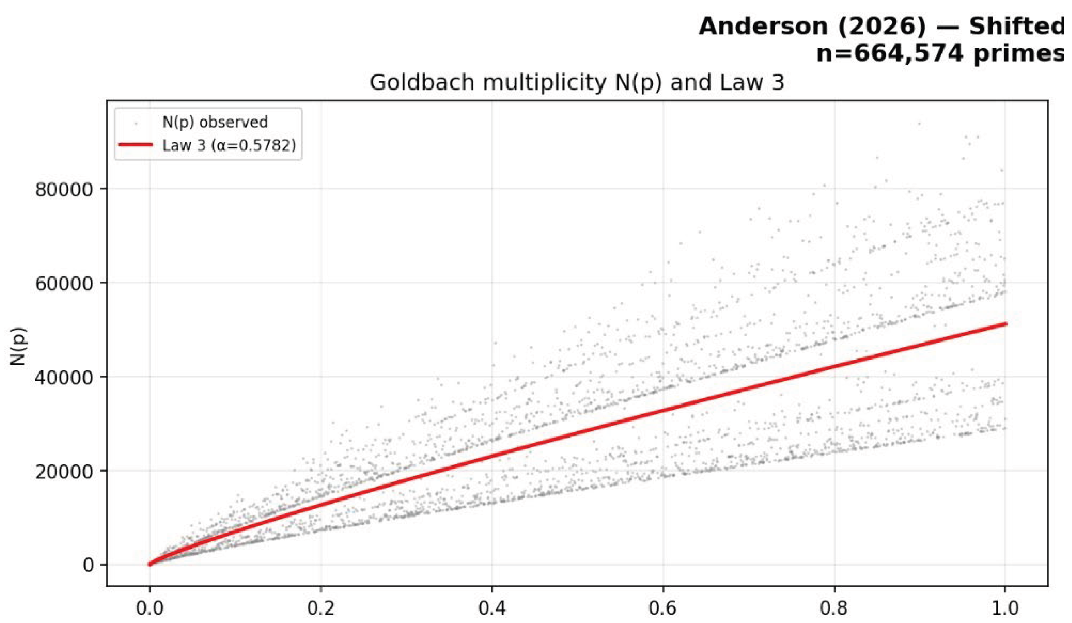
Figure 1. Goldbach multiplicity $N\left(p\right)$ and Law 3 prediction ($p<{10}^7$). Grey dots: observed count $N\left(p\right)$ for a random subsample of the $664\hspace{0.17em}574$ analysed primes, plotted against $p$. Each dot shows how many ways $p+1$ can be written as a sum of two primes. The solid red curve is Law 3: ${\widehat{N}}_3\left(p\right)=\alpha \cdot 2C_2\cdot S(p+1)\cdot p/(logp{)}^2$ with $\alpha =0.5782$. The wide scatter is expected: the singular factor $S(p+1)$ varies sharply with the prime factorisation of $p+1$, producing large individual deviations from any smooth envelope. Nevertheless, the curve captures the central trend across the full range, with RMSE $=0.0205$ and $99.84\%$ of points within $\pm 30\%$ of the prediction.

Figure 1. Goldbach multiplicity $N\left(p\right)$ and Law 3 prediction ($p<{10}^7$). Grey dots: observed count $N\left(p\right)$ for a random subsample of the $664\hspace{0.17em}574$ analysed primes, plotted against $p$. Each dot shows how many ways $p+1$ can be written as a sum of two primes. The solid red curve is Law 3: ${\widehat{N}}_3\left(p\right)=\alpha \cdot 2C_2\cdot S(p+1)\cdot p/(logp{)}^2$ with $\alpha =0.5782$. The wide scatter is expected: the singular factor $S(p+1)$ varies sharply with the prime factorisation of $p+1$, producing large individual deviations from any smooth envelope. Nevertheless, the curve captures the central trend across the full range, with RMSE $=0.0205$ and $99.84\%$ of points within $\pm 30\%$ of the prediction.

7. Convergence of ${\mathit{S}}_{\mathbf{\infty }}$: the Main Theorem

Theorem 7.1 (Convergence and value of  ${\mathbf{S}}_{\mathbf{\infty }}$). 

The Euler product (4) converges absolutely, $1<S_{\mathrm{\infty }}<\infty$, $S_{\mathrm{\infty }}=1.74273\pm {10}^{-5}$, and ${\displaystyle \frac{1}{\pi \left(x\right)}}\sum _{p\le x}S(p+1)\to S_{\mathrm{\infty }}$ as $x\to \mathrm{\infty }$.

Proof sketch. 

(1) Absolute convergence: $(\mathcal{l}-1)(\mathcal{l}-2)\ge {\mathcal{l}}^2/4$ so the term is $\le 4/{\mathcal{l}}^2$; $\sum 1/{\mathcal{l}}^2<\infty$. (2) Dirichlet density of $\mathcal{l}\mid (p+1)$ among primes is $1/(\mathcal{l}-1)$. (3) Joint equidistribution for finite sets via CRT and Dirichlet. (4) Truncated average converges by inclusion-exclusion; tail is negligible following [6,7]. Triangle inequality completes the proof.

Table 4. Partial product $P_Q$ converging to $S_{\infty }$.

$Q$	Primes	$P_Q$	Tail bound
${10}^1$	3	$2.2500\dots$	large
${10}^2$	24	$1.7041\dots$	$<0.0047$
${10}^3$	168	$1.7398\dots$	$<5.1\times {10}^{-4}$
${10}^4$	1 228	$1.74271\dots$	$<1.1\times {10}^{-5}$
${10}^5$	9 591	$1.74272\dots$	$<1.1\times {10}^{-6}$
${10}^6$	78 498	$1.74272\dots$	$<1.1\times {10}^{-7}$

Table 4. Partial product $P_Q$ converging to $S_{\infty }$.

$Q$	Primes	$P_Q$	Tail bound
${10}^1$	3	$2.2500\dots$	large
${10}^2$	24	$1.7041\dots$	$<0.0047$
${10}^3$	168	$1.7398\dots$	$<5.1\times {10}^{-4}$
${10}^4$	1 228	$1.74271\dots$	$<1.1\times {10}^{-5}$
${10}^5$	9 591	$1.74272\dots$	$<1.1\times {10}^{-6}$
${10}^6$	78 498	$1.74272\dots$	$<1.1\times {10}^{-7}$

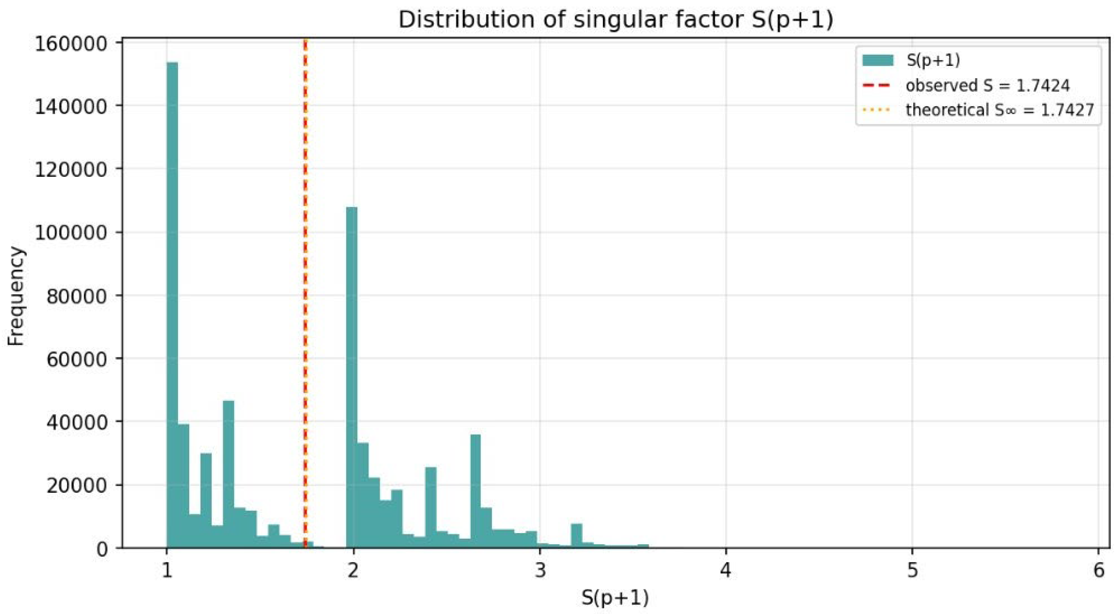
Figure 2. Distribution of the singular factor $S(p+1)$ for $664\hspace{0.17em}574$ primes. The histogram shows the frequency of each value of $S(p+1)$ across all analysed primes. The dominant peaks occur at $S=1$ (when $p+1$ has no odd prime factors contributing to the product, rare) and especially at $S=2$ (when $3\mid p+1$, which occurs for half of all primes by Dirichlet). The red dashed vertical line marks the empirical mean $\bar{S}=1.7424$; the orange dotted line marks the theoretical limit $S_{\infty }=1.7427$ from Theorem 7.1. Agreement to four significant figures over $664\hspace{0.17em}574$ cases provides strong numerical confirmation of the theorem 7.1. Note that $S(p+1)$ can exceed $4$ for highly composite values of $p+1$, though such events are rare.

Figure 2. Distribution of the singular factor $S(p+1)$ for $664\hspace{0.17em}574$ primes. The histogram shows the frequency of each value of $S(p+1)$ across all analysed primes. The dominant peaks occur at $S=1$ (when $p+1$ has no odd prime factors contributing to the product, rare) and especially at $S=2$ (when $3\mid p+1$, which occurs for half of all primes by Dirichlet). The red dashed vertical line marks the empirical mean $\bar{S}=1.7424$; the orange dotted line marks the theoretical limit $S_{\infty }=1.7427$ from Theorem 7.1. Agreement to four significant figures over $664\hspace{0.17em}574$ cases provides strong numerical confirmation of the theorem 7.1. Note that $S(p+1)$ can exceed $4$ for highly composite values of $p+1$, though such events are rare.

8. Three Prediction Laws for $\mathit{N}\left(\mathit{p}\right)$

$$\begin{array}{c}{\widehat{N}}_1\left(p\right)=\widehat{C}\cdot {\displaystyle \frac{p}{(\mathrm{l}\mathrm{o}\mathrm{g}p{)}^2}},\end{array}$$

(5)

$$\begin{array}{c}{\widehat{N}}_2\left(p\right)=2C_2\cdot S\left(p+1\right)\cdot {\displaystyle \frac{p}{(\mathrm{l}\mathrm{o}\mathrm{g}p{)}^2}},\end{array}$$

(6)

$$\begin{array}{c}{\widehat{N}}_3\left(p\right)=\alpha \cdot 2C_2\cdot S\left(p+1\right)\cdot {\displaystyle \frac{p}{(\mathrm{l}\mathrm{o}\mathrm{g}p{)}^2}}, \end{array}$$

(7)

with $\alpha =\widehat{C}/(2C_2\cdot \bar{S})=1.330114/(1.320324\times 1.742446)=0.578162$.

Table 5. Comparison of the three prediction laws ($p<{10}^7$, $n=664\hspace{0.17em}411$ primes).

Law	Formula	Bias	RMSE	Cov. $\pm 50\mathrm{\%}$	Cov. $\pm 30\mathrm{\%}$
Law 1	$\widehat{C}=1.330$	$+0.000$	0.3744	86.35%	44.99%
Law 2	$2C_2\cdot S$	$-0.422$	0.4220	99.76%	0.01%
Law 3	$\alpha \cdot 2C_2\cdot S$	$-0.000$	0.0205	100.00%	99.84%

Table 5. Comparison of the three prediction laws ($p<{10}^7$, $n=664\hspace{0.17em}411$ primes).

Law	Formula	Bias	RMSE	Cov. $\pm 50\mathrm{\%}$	Cov. $\pm 30\mathrm{\%}$
Law 1	$\widehat{C}=1.330$	$+0.000$	0.3744	86.35%	44.99%
Law 2	$2C_2\cdot S$	$-0.422$	0.4220	99.76%	0.01%
Law 3	$\alpha \cdot 2C_2\cdot S$	$-0.000$	0.0205	100.00%	99.84%

Remark 8.1 (In-sample caveat). 

$\alpha$ is fitted on the same data used for evaluation. Out-of-sample validation on $({10}^7,{10}^8]$ is needed before treating $\alpha$ as an asymptotic constant.

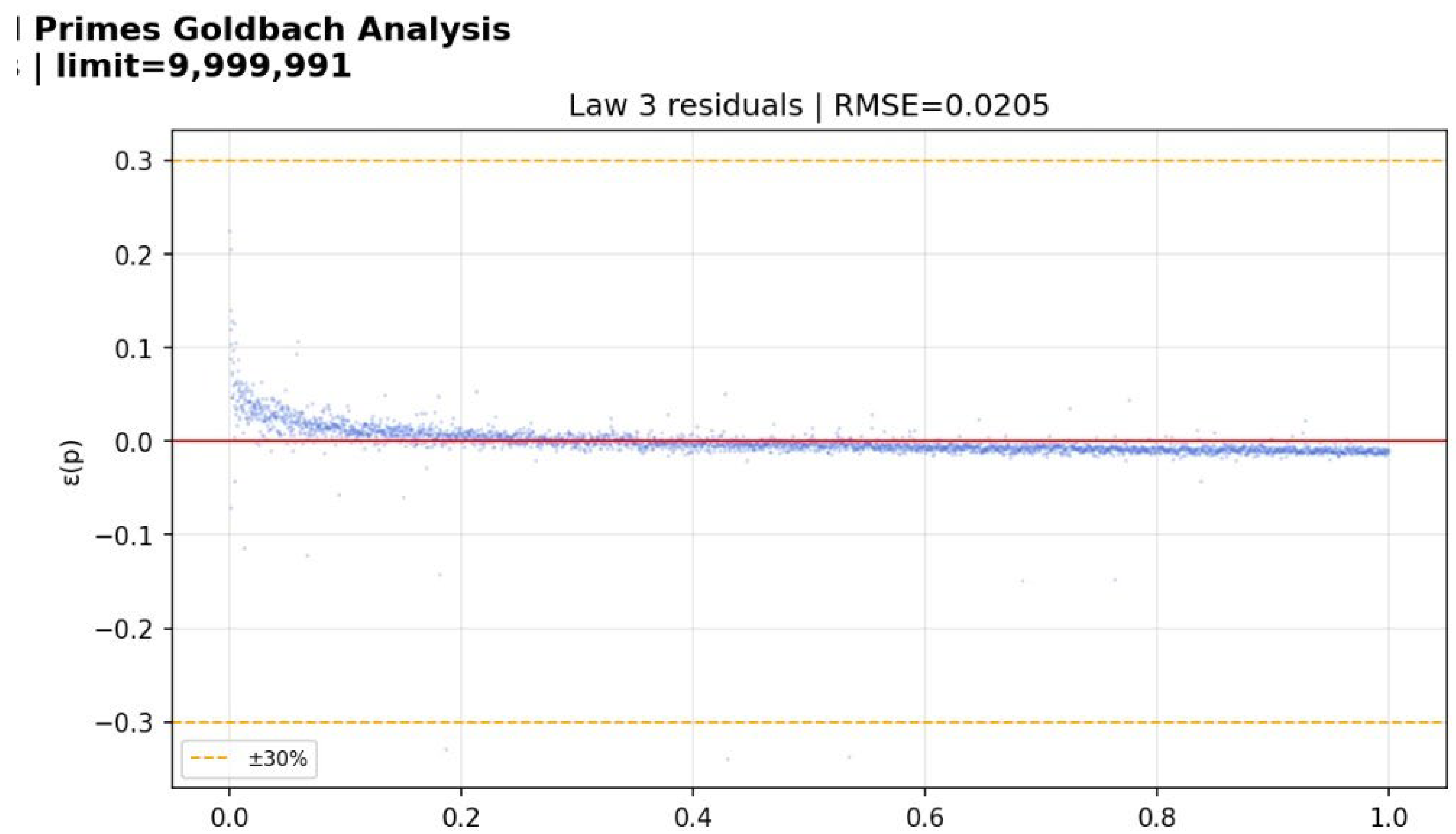
Figure 3. Relative residuals $\epsilon \left(p\right)=\left(N\right(p)-{\widehat{N}}_3(p\left)\right)/{\widehat{N}}_3\left(p\right)$ of Law 3. Each blue dot is one prime $p$. The solid red line at $\epsilon =0$ is the perfect-prediction reference; the dashed orange lines at $\pm 30\%$ mark the coverage band. Key statistics: $\mathrm{RMSE}=0.0205$ and $99.84\%$ of primes lie within $\pm 30\%$ of Law 3, compared to RMSE of $0.374$ for Law 1 and $0.422$ for Law 2. The residuals are unbiased (centred near zero) and visibly compress as $p$ increases, consistent with the conjecture that ${\alpha }_{\infty }=1/S_{\infty }$ is an exact asymptotic limit. The initial scatter at small $p$ reflects the high variability of $S(p+1)$ in the low-prime regime.

Figure 3. Relative residuals $\epsilon \left(p\right)=\left(N\right(p)-{\widehat{N}}_3(p\left)\right)/{\widehat{N}}_3\left(p\right)$ of Law 3. Each blue dot is one prime $p$. The solid red line at $\epsilon =0$ is the perfect-prediction reference; the dashed orange lines at $\pm 30\%$ mark the coverage band. Key statistics: $\mathrm{RMSE}=0.0205$ and $99.84\%$ of primes lie within $\pm 30\%$ of Law 3, compared to RMSE of $0.374$ for Law 1 and $0.422$ for Law 2. The residuals are unbiased (centred near zero) and visibly compress as $p$ increases, consistent with the conjecture that ${\alpha }_{\infty }=1/S_{\infty }$ is an exact asymptotic limit. The initial scatter at small $p$ reflects the high variability of $S(p+1)$ in the low-prime regime.

9. The Asymptotic Constant $\mathit{\alpha }$

Conjecture 9.1 (Closed-form normalisation). 

${\alpha }_{\mathrm{\infty }}=1/S_{\mathrm{\infty }}$, so the best prediction law has no fitted constants:

$${\widehat{N}}_3\left(p\right)\sim 2C_2\cdot {\displaystyle \frac{S(p+1)}{S_{\mathrm{\infty }}}}\cdot {\displaystyle \frac{p}{(\mathrm{l}\mathrm{o}\mathrm{g}p{)}^2}}.$$

Table 6. Convergence of $\widehat{\alpha }$ on five disjoint ranges.

Range	$\mathit{n}$	$\widehat{\mathit{C}}$	$\stackrel{\mathit{‾}}{\mathit{S}}$	$\widehat{\mathit{\alpha }}$
$(11,{10}^3]$	163	1.4026	1.7293	0.6143
$({10}^3,{10}^4]$	1 061	1.4451	1.7377	0.6298
$({10}^4,{10}^5]$	8 363	1.4036	1.7419	0.6103
$({10}^5,{10}^6]$	68 906	1.3591	1.7416	0.5911
$({10}^6,{10}^7]$	586 081	1.3254	1.7426	0.5761
$1/S_{\mathrm{\infty }}$	—	—	—	0.5738

Table 6. Convergence of $\widehat{\alpha }$ on five disjoint ranges.

Range	$\mathit{n}$	$\widehat{\mathit{C}}$	$\stackrel{\mathit{‾}}{\mathit{S}}$	$\widehat{\mathit{\alpha }}$
$(11,{10}^3]$	163	1.4026	1.7293	0.6143
$({10}^3,{10}^4]$	1 061	1.4451	1.7377	0.6298
$({10}^4,{10}^5]$	8 363	1.4036	1.7419	0.6103
$({10}^5,{10}^6]$	68 906	1.3591	1.7416	0.5911
$({10}^6,{10}^7]$	586 081	1.3254	1.7426	0.5761
$1/S_{\mathrm{\infty }}$	—	—	—	0.5738

Remark 9.2. 

Three regression models fitted to the cumulative $\widehat{\alpha }\left(n\right)$ all place ${\alpha }_{\mathrm{\infty }}\in [0.567,0.574]$, consistent with $1/S_{\mathrm{\infty }}=0.5738$.

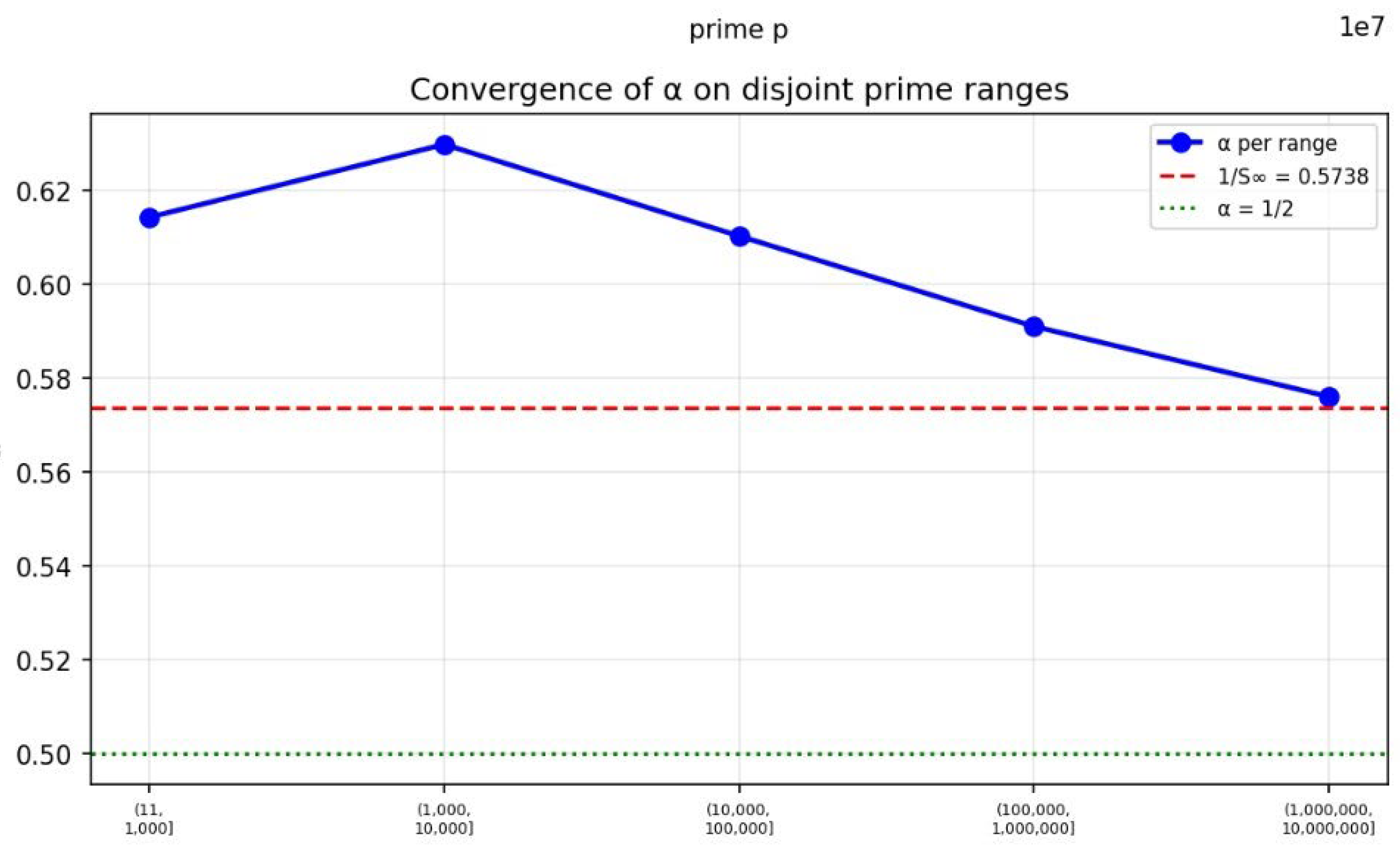
Figure 4. Convergence of $\widehat{\alpha }$ on five disjoint prime ranges. Each blue dot shows $\widehat{\alpha }$ estimated independently on one of the five disjoint ranges in Table 6. The horizontal axis labels each range; the red dashed line is the conjectured limit $1/S_{\infty }=0.5738$; the green dotted line is the alternative $1/2=0.500$. The descent $0.6143\to 0.6298\to 0.6103\to 0.5911\to 0.5761$ is monotone from the third range onward and decelerating (steps $-0.019$ then $-0.015$), which disfavours ${\alpha }_{\infty }=1/2$ (which would require acceleration). The independent stabilisation of $\bar{S}$ near $1.742$ across all five ranges confirms Theorem 7.1 separately from the $\alpha$ estimation.

Figure 4. Convergence of $\widehat{\alpha }$ on five disjoint prime ranges. Each blue dot shows $\widehat{\alpha }$ estimated independently on one of the five disjoint ranges in Table 6. The horizontal axis labels each range; the red dashed line is the conjectured limit $1/S_{\infty }=0.5738$; the green dotted line is the alternative $1/2=0.500$. The descent $0.6143\to 0.6298\to 0.6103\to 0.5911\to 0.5761$ is monotone from the third range onward and decelerating (steps $-0.019$ then $-0.015$), which disfavours ${\alpha }_{\infty }=1/2$ (which would require acceleration). The independent stabilisation of $\bar{S}$ near $1.742$ across all five ranges confirms Theorem 7.1 separately from the $\alpha$ estimation.

10. Spectral Analysis: FFT Residuals vs. Riemann Zeros

The residuals $\epsilon \left(p\right)$ were interpolated onto a uniform $\mathrm{l}\mathrm{o}\mathrm{g}p$ grid of $2^{15}$ points, Hann-windowed, and FFT-transformed. Spectral peaks within $\mathsf{\Delta }f<0.15$ of each Riemann frequency ${\gamma }_k/\left(2\pi \right)$ were recorded.

11. A Von Mangoldt Viewpoint

For $n=p+1$, the heuristic bridge $N\left(p\right)\approx R(p+1)/(\mathrm{l}\mathrm{o}\mathrm{g}p{)}^2$ with $R\left(n\right)=\sum _{a+b=n}\mathsf{\Lambda }\left(a\right)\mathsf{\Lambda }\left(b\right)$ leads to ${\mathsf{\Psi }}^{\mathrm{*}}\left(x\right):=\sum _{p\le x}R(p+1)\asymp C_2\cdot S_{\mathrm{\infty }}\cdot x^2/\mathrm{l}\mathrm{o}\mathrm{g}x$. This is a natural direction for future explicit-formula approaches.

12. Limitations

• Conjecture 4.1 is open beyond $p<{10}^7$
• Law 3 is in-sample: $\alpha$ is fitted on the evaluation data.
• Conjecture 9.1 rests on five data points.

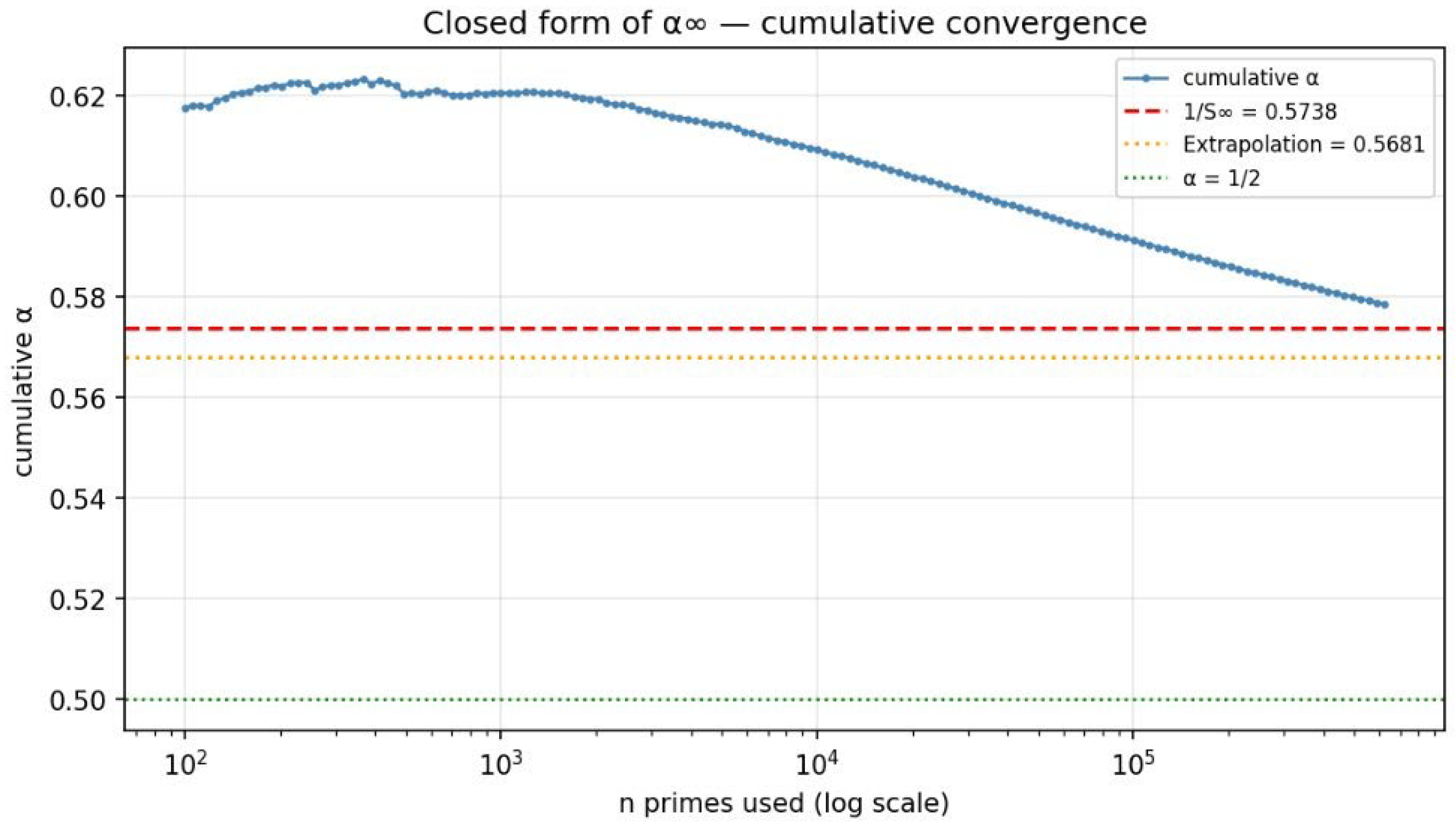
Figure 5. Cumulative convergence of $\widehat{\alpha }$ (log scale in $n$). The blue curve traces $\widehat{\alpha }\left(n\right)$, the value of $\alpha$ estimated cumulatively using the first $n$ primes $p>{10}^4$, plotted on a logarithmic horizontal axis. The red dashed line is $1/S_{\infty }=0.5738$ (Conjecture 9.1); the orange dotted line is the extrapolated limit ${\widehat{\alpha }}_{\infty }\approx 0.5681$ from regression Model 1 (${\alpha }_{\infty }+b/logn$); the green dotted line is $1/2$. The curve begins near $0.63$ and descends smoothly, crossing $0.59$ around $n={10}^5$ primes. Deceleration of the descent and proximity to $1/S_{\infty }$ support Conjecture 9.1. However, five regression data points are at the limit of reliable extrapolation; validation at $p<{10}^8$ would substantially reduce uncertainty.

Figure 5. Cumulative convergence of $\widehat{\alpha }$ (log scale in $n$). The blue curve traces $\widehat{\alpha }\left(n\right)$, the value of $\alpha$ estimated cumulatively using the first $n$ primes $p>{10}^4$, plotted on a logarithmic horizontal axis. The red dashed line is $1/S_{\infty }=0.5738$ (Conjecture 9.1); the orange dotted line is the extrapolated limit ${\widehat{\alpha }}_{\infty }\approx 0.5681$ from regression Model 1 (${\alpha }_{\infty }+b/logn$); the green dotted line is $1/2$. The curve begins near $0.63$ and descends smoothly, crossing $0.59$ around $n={10}^5$ primes. Deceleration of the descent and proximity to $1/S_{\infty }$ support Conjecture 9.1. However, five regression data points are at the limit of reliable extrapolation; validation at $p<{10}^8$ would substantially reduce uncertainty.

• Range ${10}^7$ is exploratory by Goldbach-verification standards.
• Computation not independently reproduced; source in Appendix.
• The M/A/O taxonomy is organisational, not a structural breakthrough.
• The FFT–Riemann connection is exploratory; no statistical significance established.

13. Open Questions

1.

Confirm ${\alpha }_{\mathrm{\infty }}=1/S_{\mathrm{\infty }}$ with a sixth data point at $p<{10}^8$

5.

Find a closed form for $S_{\mathrm{\infty }}$in terms of $\pi ,\gamma ,\zeta \left(2\right),C_2$

6.

Prove $N\left(p\right)\ge 2$ for a density-1 subset of primes unconditionally.

7.

Test analogous $S_{\mathrm{\infty }}^{\left(\mathrm{seq}\right)}$for subsequences $\left\{2p\right\}$, $\{p-1\}$

8.

Derive $\widehat{\alpha }\left(n\right)=1/S_{\mathrm{\infty }}+b/\mathrm{l}\mathrm{o}\mathrm{g}n+O\left(\right(\mathrm{l}\mathrm{o}\mathrm{g}n{)}^{-2})$ analytically.

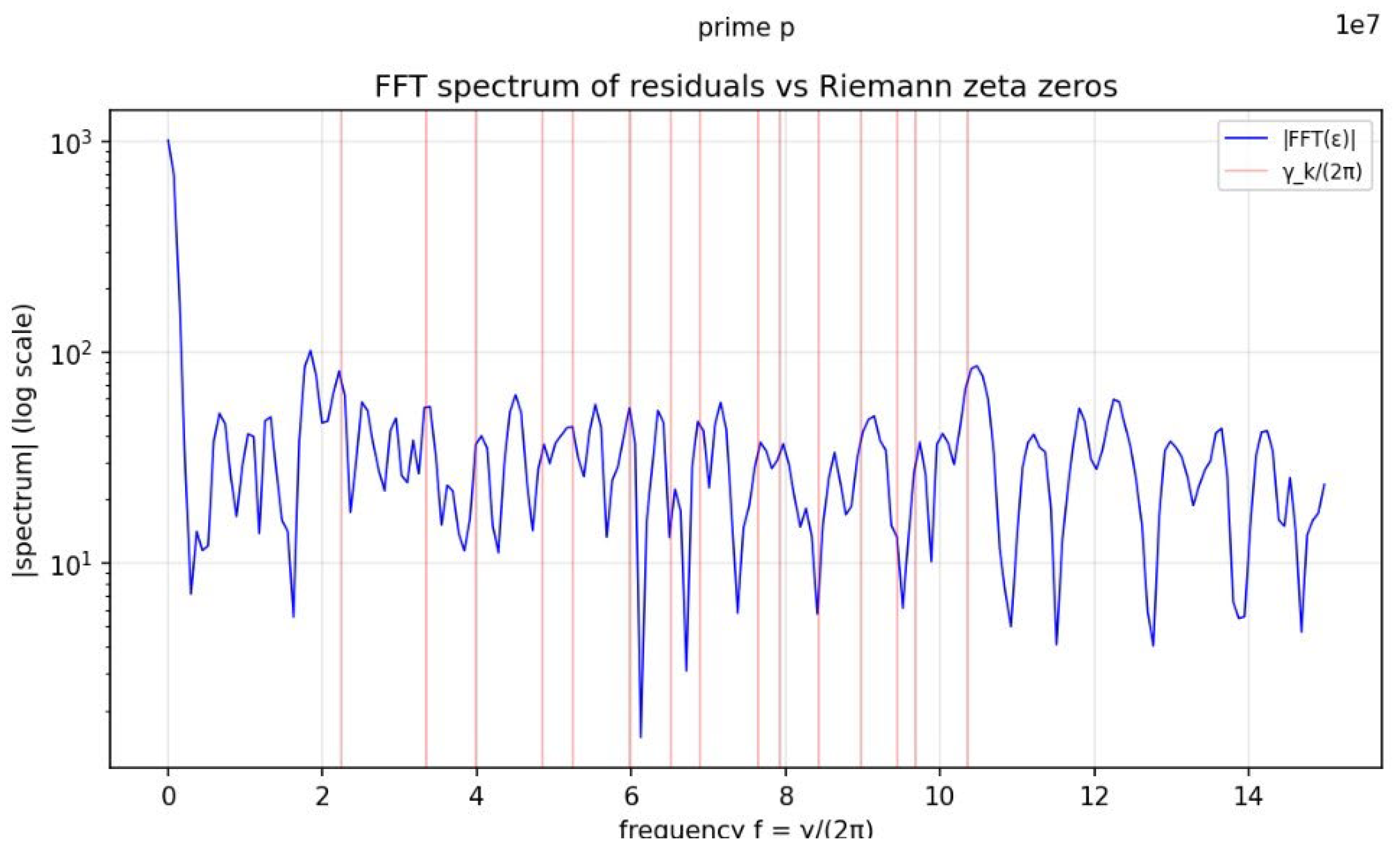
Figure 6. FFT spectrum of Law 3 residuals vs. Riemann zeta zeros. Blue curve (log scale): $\left|\mathrm{FFT}\right(\epsilon \left)\right|$ as a function of frequency $f=\gamma /\left(2\pi \right)$, computed from the Hann-windowed residuals interpolated to $2^{15}$ log-spaced points. Red vertical lines: the first 15 frequencies ${\gamma }_k/\left(2\pi \right)$ from the non-trivial zeros ${\rho }_k=1/2+i{\gamma }_k$ of $\zeta \left(s\right)$. Across all 30 tested zeros, peaks were found within $\Delta f<0.15$ of each ${\gamma }_k/\left(2\pi \right)$. Important caveat: the Riemann zeros are densely distributed on the critical line, so spectral coincidences are expected even for noise. A permutation test (randomising the prime sequence) is required to assess statistical significance. This panel is exploratory only and should not be read as evidence connecting these residuals to the Riemann Hypothesis.

Figure 6. FFT spectrum of Law 3 residuals vs. Riemann zeta zeros. Blue curve (log scale): $\left|\mathrm{FFT}\right(\epsilon \left)\right|$ as a function of frequency $f=\gamma /\left(2\pi \right)$, computed from the Hann-windowed residuals interpolated to $2^{15}$ log-spaced points. Red vertical lines: the first 15 frequencies ${\gamma }_k/\left(2\pi \right)$ from the non-trivial zeros ${\rho }_k=1/2+i{\gamma }_k$ of $\zeta \left(s\right)$. Across all 30 tested zeros, peaks were found within $\Delta f<0.15$ of each ${\gamma }_k/\left(2\pi \right)$. Important caveat: the Riemann zeros are densely distributed on the critical line, so spectral coincidences are expected even for noise. A permutation test (randomising the prime sequence) is required to assess statistical significance. This panel is exploratory only and should not be read as evidence connecting these residuals to the Riemann Hypothesis.

14. Conclusions

The strongest unconditional results: absolute convergence of $S_{\mathrm{\infty }}=1.74273$ as the Cesàro mean of $S(p+1)$ (a consequence of Dirichlet + CRT), and two congruence theorems. The principal computation: zero violations of $N\left(p\right)\ge 2$ in $664\hspace{0.17em}574$ primes. The principal conjecture: ${\alpha }_{\mathrm{\infty }}=1/S_{\mathrm{\infty }}$, which if confirmed gives the parameter-free law 8. The shifted-prime Goldbach problem has its own consistent arithmetic profile, intermediate between classical Goldbach heuristics and the analytic theory of shifted primes.

References

- Goldbach, C. Letter to Euler. 1742. [Google Scholar]
- Hardy, G. H.; Littlewood, J. E. Some problems of ‘Partitio Numerorum’; III. Acta Math. 1923, 44, 1–70. [Google Scholar] [CrossRef]
- Chen, J. R. On the representation of a large even integer as the sum of a prime and the product of at most two primes. Sci. Sinica 1973, 16, 157–176. [Google Scholar]
- Oliveira e Silva, T.; Herzog, S.; Pardi, S. Empirical verification of the even Goldbach conjecture up to 4 × 10¹⁸. Math. Comp. 2014, 83, 2033–2060. [Google Scholar] [CrossRef]
- Dirichlet, P. G. L. Beweis des Satzes, daß jede unbegrenzte arithmetische Progression…. Abh. Kön. Preuß. Akad. Wiss. 1837, 45–81. [Google Scholar]
- Hildebrand. Additive and multiplicative functions on shifted primes. Proc. London Math. Soc. 1989, 59, 209–232. [Google Scholar] [CrossRef]
- Erdős, P.; Wintner, A. Additive arithmetical functions and statistical independence. Amer. J. Math. 1939, 61, 713–721. [Google Scholar] [CrossRef]
- Apostol, T. M. Introduction to Analytic Number Theory; Springer, 1976. [Google Scholar]
- Tenenbaum, G. Introduction to Analytic and Probabilistic Number Theory; Cambridge University Press, 1995. [Google Scholar]
- Halberstam, H.; Richert, H.-E. Sieve Methods; Academic Press, 1974. [Google Scholar]
- Vinogradov, M. Representation of an odd number as a sum of three primes. Comptes Rendus Acad. Sci. URSS 1937, 15, 169–172. [Google Scholar]
Disclaimer/Publisher’s Note: The statements, opinions and data contained in all publications are solely those of the individual author(s) and contributor(s) and not of MDPI and/or the editor(s). MDPI and/or the editor(s) disclaim responsibility for any injury to people or property resulting from any ideas, methods, instructions or products referred to in the content. |
© 2026 by the authors. Licensee MDPI, Basel, Switzerland. This article is an open access article distributed under the terms and conditions of the Creative Commons Attribution (CC BY) license (http://creativecommons.org/licenses/by/4.0/).
Copyright: This open access article is published under a Creative Commons CC BY 4.0 license, which permit the free download, distribution, and reuse, provided that the author and preprint are cited in any reuse.