

Submitted:
09 March 2026
Posted:
09 March 2026
You are already at the latest version
Abstract
Metro Manila, one of the world’s most densely populated megacities, is highly vulnerable to sea-level rise due to its low-lying deltaic location, frequent tropical cyclones, and rapid anthropogenic subsidence from groundwater extraction. This study integrates historical PSMSL tide-gauge records from Manila Harbour with IPCC AR6 projections under Shared Socioeconomic Pathways, incorporating vertical land motion (VLM) and sea-level fingerprints to estimate local relative sea-level (RSL) changes. Assuming constant subsidence, cumulative VLM reaches –0.785 m by 2100 and –1.289 m by 2150. Including climatic contributions (amplified 10–20% by fingerprints, particularly under high-emission scenarios from far-field Antarctic ice loss in the western Pacific), projected RSL ranges from 1.09–1.42 m (SSP1-2.6) to 1.51–2.00 m (SSP5-8.5) by 2100, and from 1.70–2.28 m to 2.41–3.54 m by 2150. Results indicate 7.95–11.15 km² (1.2–1.8%) of land could face permanent ocean-connected inundation under high scenarios, mainly in Malabon (~18%), Navotas (~20%), and Manila (~7%). These conservative estimates (excluding aquaculture areas) are much lower than prior mid-century projections of up to 30%. Intensified chronic flooding, erosion, and saltwater intrusion threaten millions, requiring urgent integrated adaptation, groundwater regulation, and combined nature-based and engineered solutions.
Keywords:
sea-level rise
; subsidence
; Metro Manila
; IPCC projections
; coastal flooding
1. Introduction
Sea-level rise driven by climate change directly affects hundreds of millions of people living in low-elevation coastal cities. According to the IPCC Sixth Assessment Report (AR6), global mean sea level rose by 0.20 m between 1901 and 2018, at a rate of 3.7 mm/year from 2006 to 2018 [1]. Relative to the 1995–2014 baseline, projections for 2100 show likely rises of 0.28–0.55 m under SSP1-1.9 (very low emissions) and 0.63–1.01 m under SSP5-8.5 (high emissions). Due to uncertainties in some ice-sheet processes, higher values than those projected cannot be ruled out [1,2].
The main effects of sea-level rise include expanded coastal flooding, increased frequency and intensity of inundation events, accelerated coastal erosion, and saltwater intrusion [4]. The severity of these changes varies considerably at the local scale.
In some large coastal urban areas, relative sea-level rise stems not only from climatic factors but is also amplified by ground subsidence. Ground subsidence arises from various causes, some anthropogenic, such as groundwater extraction and urban loading.
The combination of sea-level rise and subsidence poses a particularly severe risk in river deltas and low-lying coastal areas. In some areas of Southeast Asia, subsidence rates frequently exceed absolute sea-level rise and constitute the most important local contribution to changes in relative sea level. More than 236 million people face heightened flood vulnerability due to subsidence combined with sea-level rise in coastal areas [5,6].
Sea-level modeling involves numerous components. Oceans, continental ice masses, glaciers, the atmosphere, and continental water storage—which operate at different spatial and temporal scales—influence these changes [7]. In general, sea-level change studies use two main data sources: tide-gauge records and satellite altimetry observations [3,8,9,10].
Regional heterogeneities of sea level must be considered when developing coastal projections, as global mean values may not fully capture this variability. Furthermore, the gravitational and rotational sea-level fingerprints induced by the redistribution of ice masses can amplify or reduce local sea-level rise, depending on the distance to the melting sources. Regions such as the western Pacific, where far-field responses to Antarctic ice loss tend to produce elevated changes in relative sea level, may be subject to an underestimation of risk when these effects are omitted [12,13].
However, satellite altimetry along coastlines at a global scale tends to underestimate the annual amplitude of sea level compared to tide-gauge records [14]. One implication is that extreme events associated with coastal flooding, expected every 20 years, could occur every 10 years in some places. Low-elevation tropical areas appear to be particularly sensitive to sea-level variability and coastal flooding [15], and the risk is amplified in areas with high population density [16]. In this regard, Metro Manila exemplifies many of the problems associated with the megalopolises of Southeast Asia. The metropolitan area hosts more than 15 million residents in a densely urbanized zone, where subsidence rates reach up to 109 mm/year [17,18]. Frequent exposure to tropical cyclones and storm surges, together with a high concentration of socioeconomically disadvantaged populations in low-elevation coastal areas, make Manila a key case for assessing sea-level rise impacts.
The study of sea level in Manila requires an approach that integrates both global mean sea-level (GMSL) projections and regional processes associated with gravitational regionalization and ocean dynamics, especially in the western Pacific, where amplifications of 10–20% have been documented [19]. Furthermore, the explicit incorporation of anthropogenic subsidence is key to estimating relative sea-level rise with greater precision.
Extending the temporal horizon beyond 2100 is relevant, given that AR6 projections indicate the persistence of sea-level rise associated with continental ice commitments during the next century [2].
This study integrates historical tide-gauge records from the Port of Manila (PSMSL, 2026; Holgate et al., 2013) with AR6 SSP projections, incorporating calibrated vertical land motion (VLM) and regional sea-level fingerprints. Based on this approach, we estimate local relative sea level up to 2150 and conduct vector spatial analysis using OpenStreetMap data to evaluate potential impacts on buildings, road infrastructure, and coastal ecosystems, as well as possible permanent flooding in Metro Manila in 2100 and 2150.
2. Methodology
This study integrates three key approaches: processing historical tide-gauge series to calibrate local subsidence, regionalization of the IPCC AR6 climate projections incorporating fingerprints, and spatial analysis of the effects on buildings, roads, and infrastructure in Metro Manila.
2.1. Study Area
Metro Manila (National Capital Region – NCR) is the political, economic, financial, and cultural hub of the Philippines. It comprises 16 highly urbanized cities and the municipality of Pateros (Figure 1), covering roughly 636 km² [20,21]. Although its official boundaries understate the true metropolitan extent, which spills into Central Luzon (Region III) and CALABARZON (Region IV-A) to form the Greater Manila Area, the NCR is delimited approximately between 14°20'N and 14°47'N latitude and between 120°56'E and 121°07'E longitude.
Administratively, the NCR is divided into four geographic districts grouping its 17 local government units:
Capital District (1st District): City of Manila.
Eastern Manila District (2nd District): Quezon City, Mandaluyong, Marikina, Pasig, San Juan.
Northern Manila District (3rd District or CAMANAVA): Caloocan, Malabon, Navotas, Valenzuela.
Southern Manila District (4th District): Las Piñas, Makati, Muntinlupa, Parañaque, Pasay, Taguig, and Pateros.
The region borders Bulacan to the north and west, Rizal and Laguna to the east, and Cavite to the south.
The 2024 Population Census recorded 14.00 million residents, up from 13.48 million in 2020 [21]. When accounting for daily commuters, floating population, and informal settlers, the effective figure likely ranges between 15 and 17 million. This yields average densities above 22,000 inhabitants/km², with peaks exceeding 50,000–60,000 inhabitants/km² in areas such as Tondo, central Manila, and parts of Quezon City [21,22].
Metro Manila occupies a low-lying (0–20 m a.s.l.) deltaic alluvial plain beside Manila Bay. Large areas are therefore vulnerable to fluvial, tidal, and storm-surge flooding. The climate follows PAGASA Type I: a distinct dry season from November to April and a long wet season from May to October, with annual rainfall of 2,000–2,500 mm. The region experiences 15–20 tropical cyclones per year, many producing significant storm surges and extreme sea levels [23,24].
The Pasig River links Laguna de Bay to Manila Bay and flows east to west across the metropolis. Its main tributary, the Marikina River, drains the eastern catchment and joins the Pasig in Pasig City. The entire Pasig-Marikina-Laguna de Bay basin (4,678 km²) drives most flooding in Metro Manila [51]. Laguna de Bay (900 km² lake; 3,820 km² watershed) normally buffers Marikina floods. However, high Manila Bay levels can reverse flow and worsen lower Pasig inundation [55]. Historical esteros, now heavily encroached and clogged by urbanization and waste, have lost their natural drainage capacity. They often amplify rather than mitigate flooding [54].
Beyond hydrometeorological risks, the 100-km West Valley Fault (WVF) poses a major seismic threat. It runs from Bulacan to Cavite and crosses Marikina, Quezon City, Makati, and Las Piñas [57]. Its southeastern segment shows accelerated aseismic creep, possibly linked to groundwater overexploitation, which may affect rupture timing [56]. A M7.2 rupture on the metropolitan segment could produce intensity VIII shaking across much of the NCR [53], with recent estimates projecting roughly 48,000 fatalities and $48 billion in economic losses given current exposure [61]. This combination of seismic, coastal, and flood hazards places Metro Manila among Southeast Asia’s most vulnerable metropolitan areas.
Coastal reclamation along Manila Bay has altered sediment dynamics and coastal morphology. PSInSAR data reveal subsidence rates of up to 6 cm/year in proposed reclamation zones and up to 9 cm/year in already developed coastal areas [59]. In these zones, seismic liquefaction risk in loose fills combines with ongoing subsidence from groundwater extraction and exposure to storm surges. The result is a particularly complex multi-hazard setting [52].
Socioeconomic patterns reinforce hazard exposure. Around 1.3 million people live in informal settlements, many concentrated in floodplains and coastal zones prone to repeated inundation [60]. From 1985 to 2015, flood-prone informal settlements grew over 50% faster than safer ones, while 85% of the NCR is now built-up [58]. These clusters are prominent along the Pasig and Marikina rivers, esteros, Tondo, and Navotas [51]. Meanwhile, high-income enclaves such as Makati and Bonifacio Global City drive income gradients that push lower-income groups toward riskier peripheries [50].
2.2. Ground Subsidence
The observed relative sea-level rise in Manila Bay is accelerated by anthropogenic ground subsidence. This process is largely driven by intensive and sustained groundwater extraction for domestic, industrial, and commercial use.
Subsidence rates range from 2 to 11 cm/year in broad coastal sectors [25]. Subsidence was particularly high in the CAMANAVA zone, north of the bay, and along the margins of Bulacan, with maxima of up to 10–15 cm/year from 2014 to 2020. These values far exceed the global mean rate of eustatic sea-level rise of approximately 3.7 mm/year [5,26].
Consequently, the effective relative rise reached approximately 2.6 cm/year or more in parts of Metro Manila. This contrasts with the historical rate of approximately 1.3 mm/year observed in the early 20th century [27,28].
Subsidence was projected assuming a constant rate, following the standard protocol adopted in previous comparative studies [5,26]. This approach constitutes a conservative “no intervention” scenario and allows for systematic comparisons between cities. However, the actual subsidence trajectory to 2100 will depend, among other factors, on the groundwater management policies that are ultimately implemented in the future.
2.3. Subsidence Sensitivity Analysis
A constant subsidence rate is a practical and methodologically acceptable assumption for a scenario without policy changes; however, it overlooks the nonlinear nature of subsidence in Metro Manila (due to soil compaction and groundwater extraction) that has accelerated in recent years.
Eco et al. (2020) [29], through radar interferometry (InSAR) for the period 2003–2011, reported rates of 20–42 mm/year in the CAMANAVA zone, values lower than the current maxima. Sulapas et al. (2024) [17], with data from 2014–2020, document extreme rates of up to 109 mm/year in Bulacan and northern bay areas, revealing a significant acceleration in the last decade associated with urban intensification and aquifer overexploitation.
Notably, the marked spatial heterogeneity of subsidence in the region is evident. The calibrated rate of ~10.1 mm/year corresponds to the specific point of the tide gauge at the tide-gauge location in Manila Harbor and reflects the conditions of the consolidated subsoil at the port front. The InSAR measurements of Sulapas et al. (2024) [17] reveal a well-documented north-south gradient: while the Port of Manila records conservative rates (~10 mm/year), the municipalities of the northern CAMANAVA zone (Malabon, Navotas, and Bulacan) present rates of 20–40 mm/year in their coastal sectors, with maxima of up to 109 mm/year in intensive extraction zones [17,18]. This difference in subsidence rates means that the projections based on the Port of Manila tide gauge represent conservative minimum estimates for the northern CAMANAVA area. In areas where subsidence is much higher (as shown by Sulapas et al., 2024), the actual relative sea-level rise may be substantially higher. In the future, using detailed subsidence maps (InSAR) at the municipal level will enable more precise, location-specific estimates.
Two recent studies provide specific data on reclaimed areas in northern Bulacan. Lomibao et al. (2024) [30], through PS-InSAR over the reclaimed zone of the Manila Bay Freeport Zone (Bay City) between 2018 and 2021, recorded a mean vertical deformation velocity of −2.06 ± 2.84 mm/year, indicating general relative stability. However, localized subsidence was detected in zones with differential settlement and adjacent constructions, reaching up to −17.52 mm/year at certain points. The authors concluded that deformation in reclaimed lands will probably continue; therefore systematic monitoring is essential as reclamation expands in the bay.
Similarly, Narca and Mabaquiao (2026) [31], applying PSI Sentinel-1 and spatial regression (OLS/GWR) in Hagonoy and Calumpit (Bulacan) for the period 2015–2021-Q1, reported subsidence rates of up to −124.5 mm/year in areas near intensive extraction points, with an average of −70.2 mm/year in a 500 m radius around pumping stations. This study confirms the statistical correlation between piezometric level, population density, and urban built volume as predictors of sinking, estimating that the annual extraction volume in Hagonoy (~9 × 10⁶ m³/year) could induce approximately 81 mm/year of subsidence.
Taken together, both studies highlight the need to account for the spatial heterogeneity of subsidence when evaluating coastal flood risk north of Manila Bay.
2.4. Data Sources
Local tide-gauge series (Manila Harbor)
The relative sea-level (RSL) records at the Port of Manila (Figure 2) were obtained from the Permanent Service for Mean Sea Level (PSMSL), a global database of tide gauges with information from approximately 2,000 stations [32,33]. Tide gauges measure the position of the sea surface relative to the terrestrial anchor point of the tide gauge itself; therefore their records integrate both oceanic variations and vertical ground movements at the observation point [34]. This is particularly relevant for actively subsiding sites like Manila, as it enables calibration of the non-climatic RSL component by differencing local and global absolute trends.
Global Mean Sea Level (GMSL) Series (1995–2014)
For the global climatic component, we used the NASA/JPL Global Mean Sea Level series from multi-mission satellite altimetry (Figure 3). This series combines observations from the TOPEX/Poseidon, Jason-1, Jason-2, Jason-3, and Sentinel-6 missions, providing global coverage of ocean topography since 1993 [9,35]. The mean rate of GMSL rise from 1993 to 2018 was 3.3 mm/year.
For the interval 1995–2014, which constitutes the IPCC AR6 reference baseline, the series is normalized to a mean of 0 mm by definition, with interannual variability of ±15–20 mm. This reference is influenced by ENSO and other climate variability.
As the global absolute sea-level (ASL) reference, we adopted the NOAA/NASA satellite altimetry series (1992–present) rather than the Church and White reconstruction (CSIRO, 2011). This choice rests on three methodological criteria.
Temporal coherence. The satellite altimetry period (1992–present) matches the temporal coverage of the Manila Harbor tide-gauge record (1992–2022), allowing direct comparison of trends over the same window. Using the 20th-century global trend from Church and White (~1.7–1.9 mm/year) would imply a lower eustatic rate typical of an earlier era, systematically overestimating VLM relative to current conditions.
Nature of measurement. Satellite altimetry directly measures ocean surface topography with quasi-global coverage without relying on spatial interpolations. In contrast, the Church and White reconstruction infers GMSL through EOF analysis from a network of tide gauges historically biased toward the North Atlantic and with limited representation in the western Pacific during the 20th century, adding uncertainty to the global reference estimate.
Representativeness of the recent subsidence. Subsidence in Manila accelerated notably from the 1960s owing to intensified groundwater extraction. Calibrating the downscaling model with the global trend from 1992–2022 (3.07 mm/year, NOAA) ensures that the estimated VLM rate (10.1 mm/year) reflects current conditions. Using a historical average would dilute the impact of recent decades of accelerated subsidence.
2.5. Sea Level Fingerprints
Regional sea-level changes are not uniform in response to global mean rise. The spatial patterns of these variations are known as sea-level fingerprints. These patterns arise from mass redistribution due to continental ice melting, which perturbs Earth’s gravitational field and causes geoid and crustal elastic deformations [36,37]. These effects, combined with Earth’s rotational response and ocean dynamics, generate regional deviations that can amplify or attenuate the eustatic rise by ±20–30% relative to the global mean [19].
The Philippine archipelago lies in the far field of Antarctic and Greenland ice-loss sources, which theoretically favors amplification of relative sea level in the western Pacific [13,38]. To quantify this effect, we applied a regional amplification factor Fr derived from the regionalized projections of Slangen et al. (2014) [19] and aligned with AR6 ocean dynamic anomaly patterns: RSLclim(t) = GMSL(t) × (1 + Fr), where RSLclim is the climatic component of RSL, GMSL is global mean rise (AR6), and Fr is the dimensionless regional fingerprint factor.
For the western tropical Pacific (5–15°N, 115–130°E), Slangen et al. (2014) [19] reported positive anomalies of 10–30% for Antarctic ice contributions, which dominate longer-term horizons. We adopted a conservative range of Fr = 0.10–0.20 for the climatic component, applied multiplicatively to the AR6 GMSL projections. This range incorporates:
- far-field gravitational effects (+5–15% from Antarctic mass loss; Mitrovica et al., 2011) [38],
- regional ocean dynamics (+5–10% from circulation variability in the western Pacific; Slangen et al., 2014; AR6 WGI) [19],
- and structural uncertainty (±5% associated with West Antarctic Ice Sheet stability).
Since gravitational fingerprint magnitude depends on ice mass lost (which increases with radiative forcing), the Fr range (0.10–0.20) is applied differentially across SSP scenarios: SSP1-2.6: 0.10–0.15; SSP2-4.5: 0.12–0.17; SSP5-8.5: 0.15–0.20. This reflects the proportionally larger Antarctic contribution to GMSL under high-emission scenarios, which intensifies far-field effects in the western Pacific [19,38].
The subranges were derived from Slangen et al. (2014)’s [19] decomposition by ice source. The Antarctic contribution (which produces the strongest far-field amplification) accounts for ~15–25% of GMSL under SSP1-2.6 but ~30–45% under SSP5-8.5, justifying higher Fr values in high-emission scenarios.
Applying this factor substantially increases the projections. For 2100 under SSP5-8.5, the climatic component rises from 0.63–1.01 m (GMSL) to 0.69–1.21 m (local RSLclim), adding 0.06–0.20 m of additional elevation. For 2150, amplification becomes more pronounced in high-emission scenarios, where Antarctic contributions grow in relative importance. This amplification, combined with persistent local subsidence, emphasizes the importance of accounting for regional geophysical heterogeneities in assessing Philippine coastal risks.
2.6. Formulation of the Integrated RSL Model
We calculate the local relative sea level (RSL) at the Port of Manila as the sum of three components: RSL(t) = GMSL_AR6(t) × (1 + Fr) + VLM(t), where
- GMSL_AR6(t) is the global mean sea-level rise projected by AR6 (m, relative to 1995–2014 baseline),
- Fr is the regional amplification factor from gravitational fingerprints and ocean dynamics (dimensionless, 0.10–0.20),
- VLM(t) is accumulated vertical land motion (m; negative = subsidence).
The regionalized climatic component is RSL_clim(t) = GMSL_AR6(t) × (1 + Fr), and the total RSL includes the non-climatic contribution: RSL_total(t) = RSL_clim(t) + VLM(t).
Uncertainty propagation is treated in a simplified analytical manner. The three main sources are: (i) uncertainty in AR6 GMSL projections, represented by the likely range (17–83 percentiles) for each SSP; (ii) uncertainty in the fingerprint factor Fr, defined by the range 0.10–0.20 from Slangen et al. (2014) [19]; (iii) uncertainty in the VLM rate, explored through three sensitivity scenarios (S1: 10.1 mm/year constant; S2: 5.03 mm/year, 50% reduction; S3: 15.06 mm/year, 50% increase).
Given that the sources of uncertainty are largely independent, the total RSL range is obtained by combining the extremes of each component. Specifically: RSL_min = GMSL_min × (1 + Fr_min) + VLM_S2, RSL_max = GMSL_max × (1 + Fr_max) + VLM_S3. This yields a deterministic envelope bounding plausible outcomes.
We converted RSL projections to permanent flood surfaces using a hydraulic connectivity flood model (ocean_flood = 1) on a ~30 m DEM (integer values in meters). The flood threshold is the median of the projected RSL range for each horizon. We evaluated DEM vertical uncertainty (±0.5 m) via envelope analysis (±0.5 m around the mean threshold), generating three spatial scenarios (conservative, medium, and optimistic) for each horizon. Intersections were computed in UTM zone 51N (EPSG:32651) to minimize areal distortion.
2.7. Climate Scenarios
Projections follow IPCC AR6 SSP scenarios [1,2], which represent different socioeconomic and emission pathways: SSP1-2.6 (low emissions, with warming below 2°C), SSP2-4.5 (intermediate emissions, ~2.7°C), and SSP5-8.5 (high emissions, >4.0°C).
The likely ranges (17–83 percentiles) of GMSL relative to the 1995–2014 baseline are:
- 0.28–0.55 m (SSP1-2.6), 0.44–0.76 m (SSP2-4.5), and 0.63–1.01 m (SSP5-8.5) for 2100;
- 0.37–0.86 m (SSP1-2.6) and 0.98–1.88 m (SSP5-8.5) for 2150.
SSP1-1.9 and SSP3-7.0 scenarios, although considered in the literature, were not included in the main analysis due to the lack of 2150 projections (SSP3-7.0) or redundancy with SSP1-2.6.
3. Results
3.1. Projections for 2100
Climate projections under moderate to high emission scenarios (SSP2-4.5 to SSP5-8.5) indicate significant impacts on Metro Manila’s coastal áreas (Table 1, Figure 4). Previous estimates from the National Adaptation Plan (2023–2050) indicate that up to 30% of the surface (~160–190 km²) could be affected by flooding between 2040 and 2050. However, our spatial análisis which exclusively considered permanent flooding with ocean connectivity and excluded already submerged zones—yields more conservative figures: 7.95 km² by 2100 and 11.15 km² by 2150 under SSP5-8.5 [27,28].
3.2. Projections for 2150
Extending projections to 2150 reveals a marked divergence between scenarios, with relative sea-level (RSL) rise at the Port of Manila reaching 1.70–2.28 m under SSP1-2.6 and 2.41–3.54 m under SSP5-8.5 (Table 2, Figure 5). Even under the low-emission pathway, RSL exceeds 1.4 m by 2150, driven primarily by the cumulative effect of land subsidence (1.289 m over 128 years at 10.1 mm/year).
3.3. Sensitivity to the Subsidence Rate
Table 3 summarizes the three subsidence scenarios. The total RSL projected for 2100 under SSP5-8.5 was as follows: S1 (constant rate, 10.1 mm/year): 1.51–2.00 m; S2 (50% reduction): 1.12–1.61 m (−0.39 m with respect to S1); and S3 (high rate, 15.1 mm/year): 1.90–2.39 m (+0.39 m with respect to S1).
Even under mitigation scenario S2, subsidence contributes 0.40–0.52 m (34–40% of total RSL), remaining the dominant risk factor. The variability between scenarios (±0.25–0.50 m) exceeded the uncertainty of the AR6 climate projections for the same temporal horizon, highlighting the weight of subsidence.
3.4. Spatial Analysis of Impacts
To evaluate the implications of the RSL projections on Metro Manila, zones of permanent flooding with hydraulic connectivity to the ocean (ocean_flood = 1) were delineated for the horizons 2100 and 2150 (SSP5-8.5 scenario) and overlaid with municipal boundaries and three OpenStreetMap vector layers [39]: buildings, natural areas, and linear infrastructure (roads, waterways, and railways). Already submerged aquaculture and open water zones in northwestern Malabon (~14.3 km²) were excluded from the flooded area calculation. Flood thresholds were set at ≤1.74 m for 2100 (median RSL from Table 1) and ≤2.72 m for 2150 (median from Table 2). Areas and lengths were calculated for geometries in EPSG:32651 (UTM zone 51N) projection.
3.4.1. Flooded Surface by Municipality
Malabon and Navotas are the most affected municipalities (Table 4). Navotas accounts for 17.2% of flooded area in 2100 and 19.9% in 2150 (Figure 6), while Malabon increases from 10.6% to 18.1%. In absolute terms, Malabon shows the largest impact (4.69 km² in 2150), followed by Manila (3.16 km²). The increase between horizons is most pronounced in Malabon (+1.94 km²), as the additional ~1 m rise expands flooding into the interior urban areas of the CAMANAVA zone. The southern municipalities (Las Piñas and Parañaque) exhibit lower absolute impact but significant relative increases (+44% and +41%, respectively).
3.4.2. Flooded Buildings
Intersecting building footprints with the flood zone identified 1,241 affected buildings, with a cumulative area of 41.70 ha. All buildings affected by 2150 lie below the 1.74 m threshold, meaning they would be permanently flooded already by 2100. Malabon has the highest number (483), mostly apartments, while Manila (Figure 7) has the largest flooded area (24.13 ha) due to larger average building size (524.5 m² vs. 159.4 m² in Malabon). Navotas ranks third with 207 buildings and 8.10 ha, predominantly residential. The southern municipalities (Las Piñas and Parañaque) show lower impact, confined to the lowest coastal strips (Table 5).
3.4.3. Flooded Natural Areas
We identified 32 affected natural areas totaling 125.29 ha. Most (104.20 ha) are water bodies (esteros, coastal rivers, drainage canals), concentrated in Navotas (64.31 ha) and Malabon (40.60 ha). Affected urban green areas comprise seven parks in Manila (5.38 ha) and two in Parañaque (0.40 ha). Affected coastal forests consist mainly of mangroves, implying direct loss of coastal protection ecosystem services. These forests cover 5.31 ha from Manila to Las Piñas (Table 6).
3.4.4. Flooded Linear Infrastructure
Unlike buildings and natural areas, linear infrastructure exhibits clear differences between 2100 and 2150. In 2100, the affected network included 1,289 segments and 106.14 km, rising to 1,567 segments and 139.22 km (31% increase) in 2150. Manila shows the largest absolute impact in both horizons (44.38 km in 2100, 53.65 km in 2150), representing 39% of the total. The increase in Manila occurs mainly in service and access streets, indicating that the additional ~1 m rise extends flooding into the interior urban fabric beyond the coastal front.
Malabon ranks second, with notable increase in waterways (+5.6 km) due to the CAMANAVA estero network. Las Piñas and Parañaque showed relative increases of 42% and 49%, respectively, with significant impact on the Manila–Cavite Expressway (CAVITEX; 5.67 km flooded in 2150). The affected railway (PNR South Main Line and LRT Line 1) totals 4.78 km in 2150. In contrast, Navotas exhibits only a marginal increase (+16%), suggesting most vulnerable infrastructure is already flooded by 2100 (Table 7).
4. Discussion
The results of this study confirm that subsidence is the dominant factor in relative sea-level rise in Metro Manila, accounting for 55–75% of total projected RSL across all analyzed scenarios. These findings align with Nicholls et al. (2021) [26] for global tropical deltas and with Shirzaei et al. (2021) [5], who identified subsidence as the primary local driver of relative sea-level change in coastal areas affecting over 236 million people. Subsidence has direct implications for adaptation policy: the primary lever for reducing short- to medium-term coastal risk is effective local groundwater management [6,40].
RSL projections for the Port of Manila (1.09–2.00 m in 2100; 2.41–3.54 m in 2150 under SSP5-8.5) are higher than regional climatic-only estimates (~0.5–1.0 m) from Becker et al. (2024) [41]. These differences arise from the explicit incorporation of locally calibrated VLM using PSMSL records [32,33] and gravitational fingerprints [19]. The projections also exceed AR6 GMSL likely ranges (0.63–1.01 m under SSP5-8.5 for 2100; [1,2]), highlighting the dominance of local and regional factors over global mean values [8,10].
In contrast, permanent flooding estimates here (7.95–11.15 km²) are much lower than the ~30% surface area projected by the National Adaptation Plan (2023–2050) and Philippine Climate Change Assessment (2024) [27,28]. This discrepancy reflects differing analytical thresholds rather than a contradiction: the National Plan quantifies exposure to recurrent extreme events with defined return periods, whereas this study focuses on permanent flooding with ocean connectivity and excludes already submerged aquaculture zones [39]. Both approaches are complementary and essential for a comprehensive coastal risk assessment [42].
Gravitational fingerprints amplify the climatic component of sea level by 10–20% in the western Pacific. This expected effect stems from the Philippine archipelago’s position in the far field of Antarctic and Greenland ice-loss sources [36,37,38]. Amplification is not constant and intensifies with increasing radiative forcing. Under high-emission scenarios, the Antarctic contribution to GMSL is proportionally greater (30–45% under SSP5-8.5 versus 15–25% under SSP1-2.6), intensifying far-field responses [12,19]. For 2100 under SSP5-8.5, the local climatic component rises from 0.63–1.01 m (GMSL) to 0.72–1.21 m after applying the amplification factor, adding 0.06–0.20 m of additional elevation.
Projections for Manila are more pronounced than those for other deltaic megacities in South Asia. Jakarta represents the most extreme case, with subsidence rates up to 25–28 cm/year in the north [40,43], contributing to the decision to relocate the capital to Nusantara. Manila’s estimated VLM rate (10.1 mm/year) is clearly lower than Jakarta’s maxima. In Bangkok, subsidence rates fell from 12 cm/year in the 1980s to 1–2 cm/year after regulating groundwater extraction [44]. In Ho Chi Minh City, current subsidence rates range from 1 to 8 cm/year [26,45]. In all three cities, subsidence exceeds the climatic eustatic component [5], confirming a common pattern in tropical deltas where groundwater extraction is a primary cause of sinking [6,40].
The sensitivity analysis supports this conclusion. Variability across subsidence scenarios S1–S3 (±0.39 m for 2100 under SSP5-8.5) exceeds the uncertainty in AR6 climate projections for the same horizon [2]. Even under the mitigation scenario S2 (50% reduction), subsidence contributes 0.40–0.52 m (34–40% of total RSL).
Spatial analysis highlights concentrated vulnerability. Malabon and Navotas reach 18% and 20% of their land surface permanently flooded by 2150, respectively, in zones where population density exceeds 22,000 inhabitants/km² [21,22]. The 1,241 vulnerable buildings lie below the 2100 threshold (≤1.74 m), indicating that permanent building flooding is a near-term (21st-century) reality. Linear infrastructure exhibits a 31% increase between 2100 and 2150, including 4.78 km of railway (PNR South Main Line and LRT Line 1) and 5.67 km of highway (CAVITEX) in 2150. The CAMANAVA zone contains 80% of vulnerable buildings and waterways, warranting priority in future land-use planning [18,24].
Projections are referenced to mean sea level and do not incorporate tidal or storm surges. In Manila Bay, the mixed semidiurnal tidal regime produces a mean range of 1.0–1.2 m [23], meaning actual water levels may exceed projected thresholds by 0.5–0.6 m during spring high tides.
The DEM’s vertical resolution (~30 m, integer values) imposes ±0.5 m uncertainty, comparable to the mean tidal range amplitude. The resulting envelope (4.2–12.4 km² by 2100) indicates that even in the most favorable scenario, >4 km² of urban fabric would be permanently flooded.
The methodology has several limitations. The linear subsidence projection, although standard in comparative literature [5,26], overlooks potential nonlinearities from progressive aquifer compaction or future extraction policy changes. The fingerprint factor is applied as a deterministic multiplier of GMSL [12]. OpenStreetMap layers [39] have limitations, particularly underrepresentation of informal settlements, which are often the most vulnerable. Thus, estimates for affected buildings and infrastructure are conservative. Finally, 2150 projections are subject to substantial uncertainty regarding West Antarctic Ice Sheet stability [46,47,48,49] and should be viewed as exploratory scenarios.
The results indicate that climate change adaptation in Metro Manila will require actions at multiple time scales. Immediate priorities include regulating groundwater extraction. Conservation and restoration of mangroves as nature-based coastal protection is gaining increasing importance [42]. Immediate priorities include proven local interventions feasible within urban planning timeframes [40,44]. However, the dominance of subsidence relative to the climatic component does not diminish the urgency of emission mitigation [1]. Metro Manila represents one of the clearest examples of compound climatic and anthropogenic risks in the Global South [5,26], where effective interventions are urgently needed.
5. Conclusions
This study integrates local tide-gauge records (PSMSL), IPCC AR6 climate projections regionalized through gravitational fingerprints, and spatial analysis of urban infrastructure in Metro Manila, extending the temporal horizon to 2150.
The results show that anthropogenic ground subsidence is the dominant factor in relative sea-level rise in Metro Manila, exceeding the climatic contribution in all analyzed scenarios.
Gravitational fingerprints and regional ocean dynamics amplify the climatic component of sea level in the western Pacific. These factors are essential in regional assessments to avoid underestimating coastal risks from climate change.
The spatial analysis reveals a clear concentration of vulnerability in the CAMANAVA municipalities—particularly Malabon and Navotas—and in Manila’s coastal districts. This pattern should guide the prioritization of adaptation strategies and land-use planning in these areas over the coming decades.
Metro Manila exemplifies the convergence of climatic and anthropogenic risks typical of deltaic megacities in the Global South. The findings suggest that adaptation strategies will require a combination of sustainable groundwater management, nature-based coastal protection solutions, and periodic updating of projections as new IPCC assessment cycles emerge. The dominance of subsidence over the climatic component in relative sea-level rise does not diminish the urgency of emissions mitigation.
Author Contributions
A.D.I.-M.: Conceptualization, Data curation, Formal analysis, Investigation, Methodology, Software, Visualization, Writing – original draft, Writing – review & editing; L.M.S.-M.: Formal analysis, Methodology, Software, Writing – review & editing; D.M.-C.: Methodology, Software, Writing – review & editing; F.B.-S.: Supervision, Writing – review & editing. All authors have read and agreed to the published version of the manuscript.
Funding
This research received no external funding.
Acknowledgments
The authors acknowledge the Permanent Service for Mean Sea Level (PSMSL) for providing tidal gauge data, OpenStreetMap (OSM) contributors for the open geographic data, and the QGIS Development Team for the open-source GIS software used in this study.
Conflicts of Interest
The authors declare no conflict of interest.
References
- IPCC. Climate Change 2021: The Physical Science Basis; Cambridge University Press: Cambridge, UK, 2021. [Google Scholar]
- Fox-Kemper, B.; Hewitt, H.T.; Xiao, C.; et al. Ocean, cryosphere and sea level change. In Climate Change 2021: The Physical Science Basis; Cambridge University Press: Cambridge, UK, 2021; pp. 1211–1362. [Google Scholar]
- IPCC. Climate Change 2022: Impacts, Adaptation and Vulnerability; Cambridge University Press: Cambridge, UK, 2022. [Google Scholar]
- Fraile-Jurado, P.; Álvarez-Francoso, J.I.; Guisado-Pintado, E.; Sánchez-Carnero, N.; Ojeda-Zújar, J.; Leatherman, S.P. Mapping inundation probability due to increasing sea level rise along El Puerto de Santa María (SW Spain). Nat. Hazards 2017, 87, 581–598. [Google Scholar] [CrossRef]
- Shirzaei, M.; Bürgmann, R.; Fielding, E.J.; Hensley, S.; Hudnut, K.; Lanari, R.; et al. Measuring, modelling, and projecting coastal land subsidence. Nat. Rev. Earth Environ. 2021, 2, 40–58. [Google Scholar]
- Minderhoud, P.S.J.; Middelkoop, H.; Erkens, G.; Stouthamer, E. Groundwater extraction may drown mega-delta. Environ. Res. Commun. 2020, 2, 011005. [Google Scholar] [CrossRef]
- Cazenave, A.; Llovel, W. Contemporary sea-level rise. Annu. Rev. Mar. Sci. 2010, 2, 145–173. [Google Scholar] [CrossRef]
- Dangendorf, S.; Marcos, M.; Wöppelmann, G.; Conrad, C.P.; Frederikse, T.; Riva, R. Reassessment of the 20th century global mean sea level rise. Proc. Natl. Acad. Sci. USA 2017, 114, 5946–5951. [Google Scholar] [CrossRef] [PubMed]
- Nerem, R.S.; et al. Climate-change-driven accelerated sea-level rise detected during the altimeter era. Proc. Natl. Acad. Sci. USA 2018, 115, 2022–2025. [Google Scholar] [CrossRef]
- Cazenave, A.; Le Cozannet, G. Sea-level rise and its coastal impacts. Earth’s Future 2018, 2, 15–34. [Google Scholar] [CrossRef]
- Church, J.A.; White, N.J. Sea-level rise from the late 19th to the early 21st century. Surv. Geophys. 2011, 32, 585–602. [Google Scholar] [CrossRef]
- Mitrovica, J.X.; Hay, C.C.; Kopp, R.E.; Harig, C.; Latychev, K. Quantifying the sensitivity of sea level change in coastal localities. J. Clim. 2018, 31, 3701–3709. [Google Scholar] [CrossRef]
- Hay, C.C.; Morrow, E.; Kopp, R.E.; Mitrovica, J.X. Probabilistic reanalysis of twentieth-century sea-level rise. Nature 2015, 517, 481–484. [Google Scholar] [CrossRef]
- Qu, Y.; Jevrejeva, S.; Jackson, L.P.; Moore, J.C. Coastal sea level rise around the China seas. Glob. Planet. Chang. 2019, 172, 454–463. [Google Scholar] [CrossRef]
- Jevrejeva, S.; Williams, J.; Vousdoukas, M.I.; et al. Future sea-level rise dominates the changes in the worst-case extreme sea levels along the global coastline by 2100. Environ. Res. Lett. 2023, 18, 024037. [Google Scholar] [CrossRef]
- Widlansky, M.J.; Long, X.Y.; Schloesser, F. The increase in sea-level variability with ocean warming is associated with the nonlinear thermal expansion of seawater. Commun. Earth Environ. 2020, 1, 9. [Google Scholar] [CrossRef]
- Sulapas, J.J.; Ybañez, A.A.; Marasigan, K.M.; Grageda, J.M.B.; Lagmay, A.M.F.A. Ground subsidence in major Philippine metropolitan cities from 2014 to 2020. Int. J. Appl. Earth Obs. Geoinf. 2024, 133, 104107. [Google Scholar] [CrossRef]
- Lagmay, A.M.F.A.; Santiago, J.T.; Mendoza, J.E. Mainstreaming climate and disaster risk assessment in the comprehensive land use plan. In Climate Emergency in the Philippines; Springer Singapore: Singapore, 2024; pp. 279–302. [Google Scholar] [CrossRef]
- Slangen, A.B.A.; Carson, M.; Katsman, C.A.; van de Wal, R.S.W.; Köhl, A.; Vermeersen, L.L.A.; Stammer, D. Projecting twenty-first-century regional sea-level changes. Clim. Chang. 2014, 124, 317–332. [Google Scholar] [CrossRef]
- MMDA. Metro Manila Development Authority Annual Report 2023; Metropolitan Manila Development Authority: Mandaluyong, Philippines, 2023. [Google Scholar]
- PSA. 2024 Census of Population and Housing; Philippine Statistics Authority: Quezon City, Philippines, 2025. [Google Scholar]
- World Bank. Philippines Urbanization Review: Fostering Competitive, Sustainable, and Inclusive Cities; World Bank Group: Washington, DC, USA, 2023. [Google Scholar]
- PAGASA. Climate and Agromet Data Section; Philippine Atmospheric, Geophysical and Astronomical Services Administration: Quezon City, Philippines, 2024. [Google Scholar]
- JICA. Roadmap for Transport Infrastructure Development for Metro Manila and Its Surrounding Areas; Japan International Cooperation Agency: Tokyo, Japan, 2022. [Google Scholar]
- Espiritu, K.W.; Reyes, C.J.; Benitez, T.M.; Tokita, R.C.; Galvez, L.J.; Ramirez, R. Sentinel-1 interferometric synthetic aperture radar (InSAR) reveals continued ground deformation in and around Metro Manila, Philippines. Nat. Hazards 2022, 114, 3139–3161. [Google Scholar] [CrossRef]
- Nicholls, R.J.; Lincke, D.; Hinkel, J.; Brown, S.; Vafeidis, A.T.; Meyssignac, B.; et al. A global analysis of subsidence, relative sea-level change, and coastal flood exposure. Nat. Clim. Chang. 2021, 11, 338–342. [Google Scholar] [CrossRef] [PubMed]
- National Adaptation Plan; Climate Change Commission: Manila, Philippines, 2023.
- Philippine Climate Change Assessment. In Physical Science Basis; Oscar M. Lopez Center, PAGASA, Climate Change Commission: Manila, Philippines, 2024.
- Eco, R.C.; Lagmay, A.M.F.; Largo, J.P. InSAR-derived land subsidence in Metro Manila, Philippines using ALOS PALSAR images. Philipp. J. Sci. 2020, 149, 87–97. [Google Scholar] [CrossRef]
- Lomibao, A.L.; Leal, G.A.; Mabaquiao, L.C.; Reyes, R.B. Ground deformation monitoring of reclaimed lands along Manila Bay Freeport Zone using PS-InSAR technique. Int. Arch. Photogramm. Remote Sens. Spat. Inf. Sci. 2024, XLVIII-4/W8-2023, 335–342. [Google Scholar] [CrossRef]
- Narca, A.M.Y.; Mabaquiao, L.C.S. Correlation of land subsidence with groundwater extraction and urbanization in Hagonoy and Calumpit, Bulacan from 2015 to 2021-Q1. Int. Arch. Photogramm. Remote Sens. Spat. Inf. Sci. 2026, XLVIII-5/W4-2025, [in press]. [Google Scholar]
- Holgate, S.J.; Matthews, A.; Woodworth, P.L.; Rickards, L.J.; Tamisiea, M.E.; Bradshaw, E.; et al. New data systems and products at the Permanent Service for the Mean Sea Level. J. Coast. Res. 2013, 29, 493–504. [Google Scholar] [CrossRef]
- Permanent Service for Mean Sea Level (PSMSL). Tide Gauge Data. Available online: http://www.psmsl.org/data/obtaining (accessed on 8 December 2025).
- Cazenave, A.; Remy, F. Sea level and climate: Measurements and causes of changes. WIREs Clim. Chang. 2011, 2, 647–662. [Google Scholar] [CrossRef]
- Beckley, B.D.; Callahan, P.S.; Hancock, D.W.; Mitchum, G.T.; Ray, R.D. On the “Cal-Mode” Correction to TOPEX Satellite Altimetry and Its Effect on the Global Mean Sea Level Time Series. J. Geophys. Res. Oceans 2017, 122, 8371–8384. [Google Scholar] [CrossRef]
- Mitrovica, J.X.; Tamisiea, M.E.; Davis, J.L.; Milne, G.A. Recent mass balance of polar ice sheets inferred from patterns of global sea-level change. Nature 2001, 409, 1026–1029. [Google Scholar] [CrossRef]
- Tamisiea, M.E.; Mitrovica, J.X.; Davis, J.L. A method for detecting rapid mass flux of small glaciers using local sea-level variations. Earth Planet. Sci. Lett. 2003, 216, 353–361. [Google Scholar] [CrossRef]
- Mitrovica, J.X.; Gomez, N.; Morrow, E.; Hay, C.; Latychev, K.; Tamisiea, M.E. On the robustness of the predictions of sea-level fingerprints. Geophys. J. Int. 2011, 187, 729–742. [Google Scholar] [CrossRef]
- OpenStreetMap Contributors. Planet Dump. Available online: https://planet.openstreetmap.org (accessed on 20 December 2024).
- Erkens, G.; Bucx, T.; Dam, R.; de Lange, G.; Lambert, J. Sinking coastal cities. Proc. IAHS 2015, 372, 189–198. [Google Scholar] [CrossRef]
- Becker, M.; Karpytchev, M.; Papa, F. Hotspots of relative sea-level rise in the Tropics. In Tropical and Subtropical Coastal Zones; Springer: Cham, Switzerland, 2024; pp. 203–231. [Google Scholar]
- Oppenheimer, M.; Glavovic, B.C.; Hinkel, J.; van de Wal, R.; Magnan, A.K.; Abd-Elgawad, A.; et al. Sea-level rise and its implications for low-lying islands, coasts, and communities. In IPCC Special Report on the Ocean and Cryosphere; Cambridge University Press: Cambridge, UK, 2019; pp. 321–445. [Google Scholar] [CrossRef]
- Abidin, H.Z.; Andreas, H.; Gumilar, I.; Fukuda, Y.; Pohan, Y.E.; Deguchi, T. Land subsidence of Jakarta (Indonesia) and its relation with urban development. Nat. Hazards 2011, 59, 1753–1771. [Google Scholar] [CrossRef]
- Phien-wej, N.; Giao, P.H.; Nutalaya, P. Land subsidence in Bangkok, Thailand. Eng. Geol. 2006, 82, 187–201. [Google Scholar] [CrossRef]
- Minderhoud, P.S.J.; Erkens, G.; Pham, V.H.; Bui, V.T.; Erban, L.; Kooi, H.; Stouthamer, E. Impacts of 25 years of groundwater extraction on subsidence in the Mekong delta, Vietnam. Environ. Res. Lett. 2017, 12, 064006. [Google Scholar] [CrossRef]
- DeConto, R.M.; Pollard, D. Contribution of Antarctica to past and future sea-level rise. Nature 2016, 531, 591–597. [Google Scholar] [CrossRef]
- DeConto, R.M.; Pollard, D.; Alley, R.B.; Velicogna, I.; Gasson, E.; Gomez, N.; et al. The Paris Climate Agreement and future sea-level rise from Antarctica. Nature 2021, 593, 83–89. [Google Scholar] [CrossRef] [PubMed]
- Edwards, T.L.; Brandon, M.A.; Durand, G.; Edwards, N.R.; Golledge, N.R.; Holden, P.B.; et al. Revisiting Antarctic ice loss due to marine ice-cliff instability. Nature 2019, 566, 58–64. [Google Scholar] [CrossRef]
- Edwards, T.L.; Nowicki, S.; Marzeion, B.; Hock, R.; Goelzer, H.; Seroussi, H.; et al. Projected land ice contributions to twenty-first-century sea level rise. Nature 2021, 593, 74–82. [Google Scholar] [CrossRef]
- Choi, N. Metro Manila through the gentrification lens: Disparities in urban planning and displacement risks. Urban Studies 2016, 53, 577–592. [Google Scholar] [CrossRef]
- Dulawan, J.M.T.; Imamura, Y.; Amaguchi, H. Integrating social vulnerability to flood risk assessment in Metro Manila. River 2024, 3, 373–388. [Google Scholar] [CrossRef]
- Eco, R.C.; Lagmay, A.M.F.; Punongbayan, R.S. Manila Bay reclamation and its impacts on the people and environment. AGU Fall Meeting Abstracts 2018, PA43E-1385. 2018.
- JICA/PHIVOLCS. Earthquake Impact Reduction Study for Metropolitan Manila; JICA: Tokyo, Japan, 2004. [Google Scholar]
- Lagmay, A.M.F.; Mendoza, J.; Cipriano, F.; Delmendo, P.A.; Lacsamana, M.N.; Moises, M.A.; Pellejera, N.; Punay, K.N.; Sabio, G.; Santos, L. Street floods in Metro Manila and possible solutions. J. Environ. Sci. 2017, 59, 39–47. [Google Scholar] [CrossRef] [PubMed]
- NAPHRS/JICA. The Hydrological and Geophysical Environment of Metro Manila; NIED: Tsukuba, Japan, 2009. [Google Scholar]
- Rimando, R.E.; Rimando, J.M.; Ong, P.J.L.; Aguilar, P.J.L.; Gojo Cruz, A.P.S. Spatial and temporal variation of aseismic creep along the West Valley Fault. Front. Earth Sci. 2022, 10, 935161. [Google Scholar] [CrossRef]
- Rimando, R.E.; et al. Earthquake history and rupture extents along the Valley Fault System. GeoHazards 2025, 6, 23. [Google Scholar] [CrossRef]
- Rivera, A.T.; et al. Social drivers of flood vulnerability in Metro Manila. Water 2024, 16, 799. [Google Scholar] [CrossRef]
- Rodolfo, K.S. On the geological hazards that threaten existing and proposed reclamations of Manila Bay. Sci. Eng. J. 2014, 7, 228–240. [Google Scholar]
- World Bank. Philippines Urbanization Review; World Bank: Washington, DC, USA, 2017. [Google Scholar]
- World Bank. Seismic Resilience in Metro Manila: Accessing Healthcare after a Catastrophic Earthquake; World Bank Blogs: Washington, DC, USA, 2024. [Google Scholar]
Figure 1.
Study area: Metro Manila (National Capital Region), Philippines. The map shows the 17 local government units.
Figure 1.
Study area: Metro Manila (National Capital Region), Philippines. The map shows the 17 local government units.
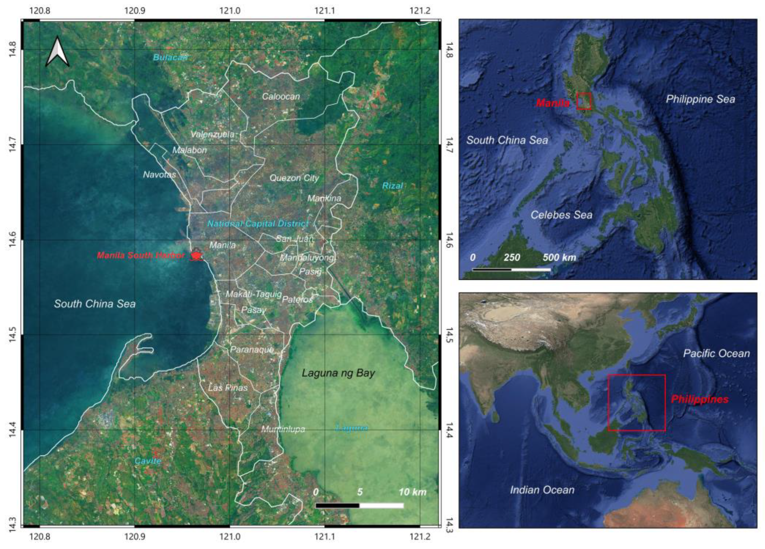
Figure 2.
Historical sea-level records at the Port of Manila. (a) Annual mean relative sea level (RSL) from the PSMSL tide-gauge record (1901–2022).
Figure 2.
Historical sea-level records at the Port of Manila. (a) Annual mean relative sea level (RSL) from the PSMSL tide-gauge record (1901–2022).
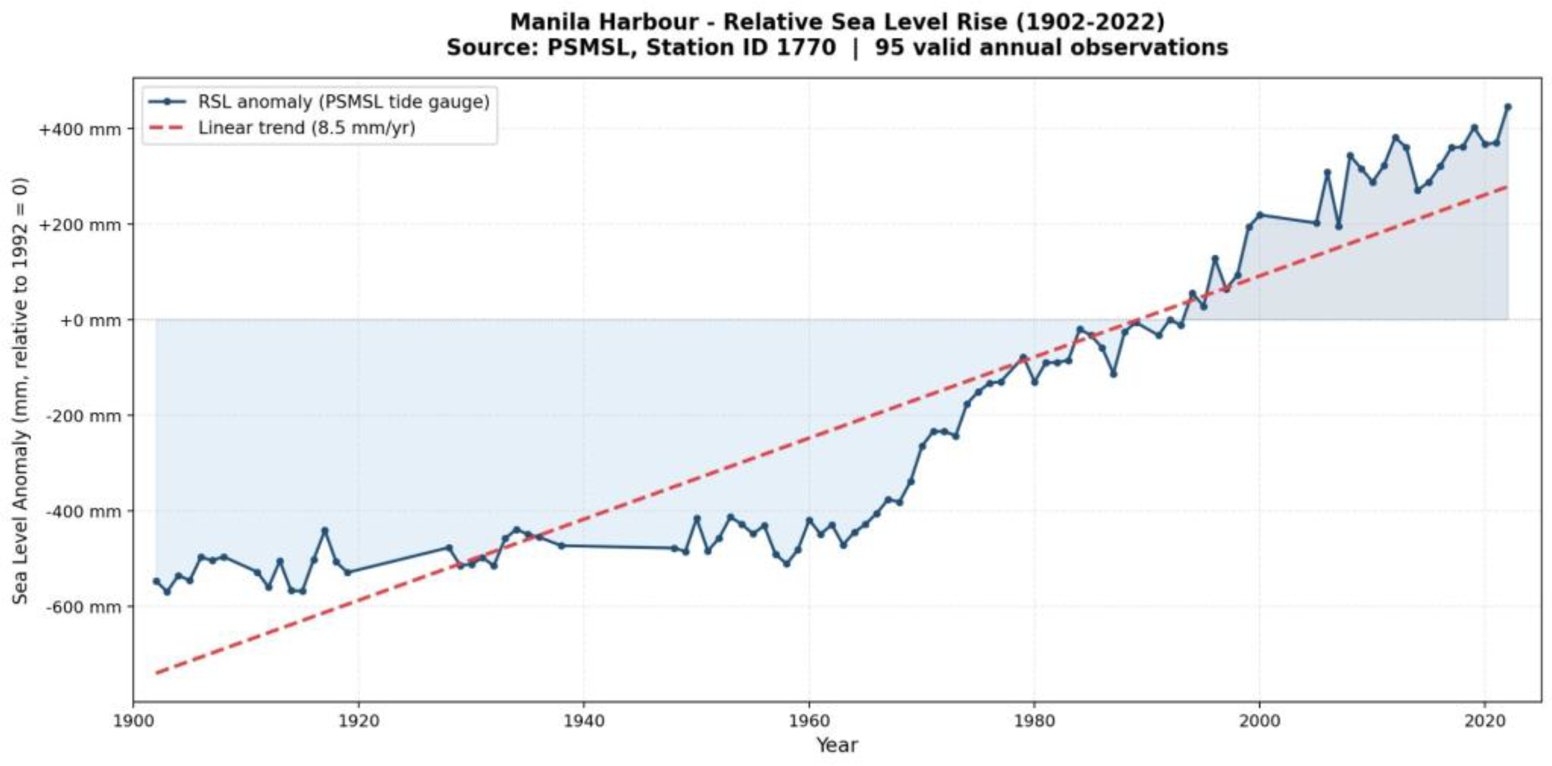
Figure 3.
Global mean sea level (GMSL) from multi-mission satellite altimetry (1993–2024), relative to 1992 baseline.
Figure 3.
Global mean sea level (GMSL) from multi-mission satellite altimetry (1993–2024), relative to 1992 baseline.
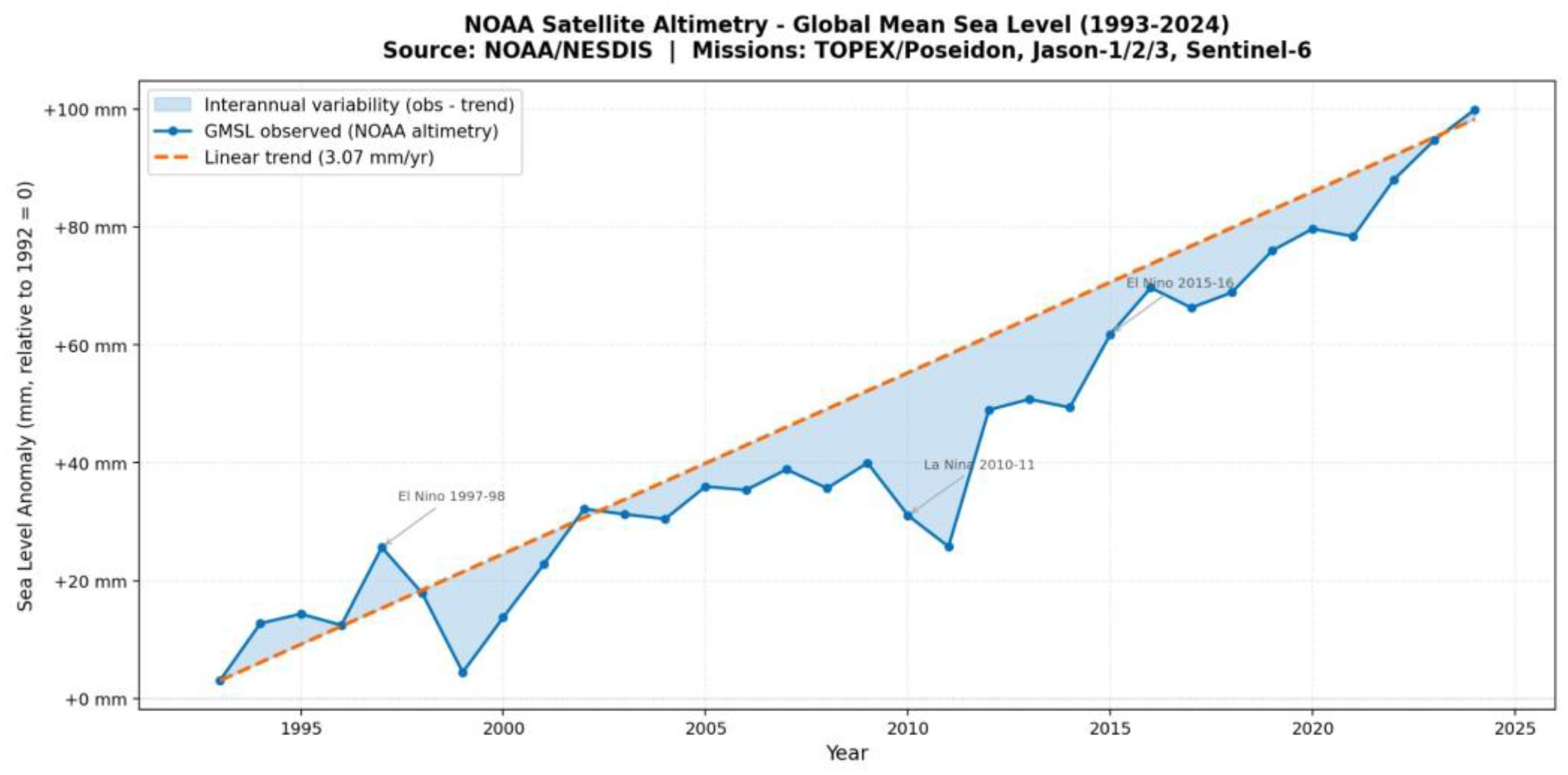
Figure 4.
Observed and projected relative sea level (RSL) at the Port of Manila to 2100 under SSP1-2.6, SSP2-4.5, and SSP5-8.5.
Figure 4.
Observed and projected relative sea level (RSL) at the Port of Manila to 2100 under SSP1-2.6, SSP2-4.5, and SSP5-8.5.
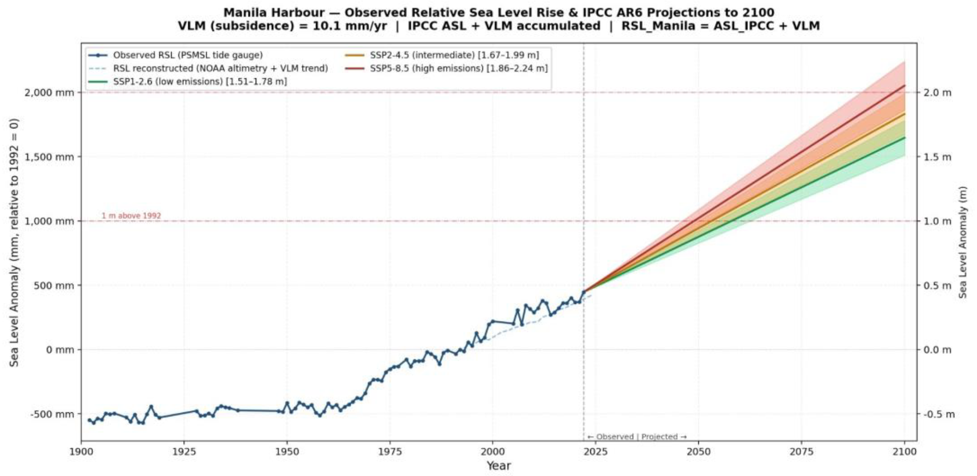
Figure 5.
Projected relative sea level (RSL) at the Port of Manila to 2150 under SSP1-2.6 and SSP5-8.5 (likely range). VLM: 10.1 mm/year.
Figure 5.
Projected relative sea level (RSL) at the Port of Manila to 2150 under SSP1-2.6 and SSP5-8.5 (likely range). VLM: 10.1 mm/year.
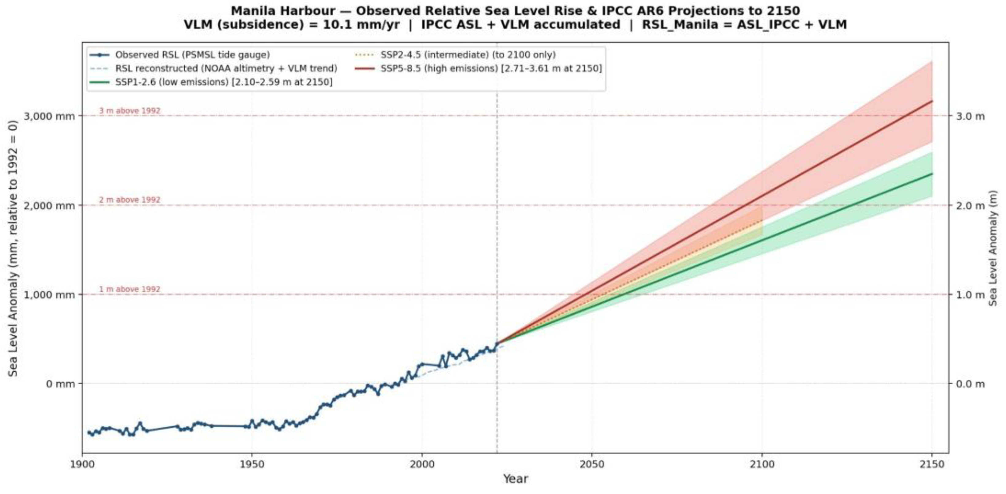
Figure 6.
Permanent flood zone (2150, SSP5-8.5) in the CAMANAVA district along the Tullahan River. Inset: location within Metro Manila.
Figure 6.
Permanent flood zone (2150, SSP5-8.5) in the CAMANAVA district along the Tullahan River. Inset: location within Metro Manila.
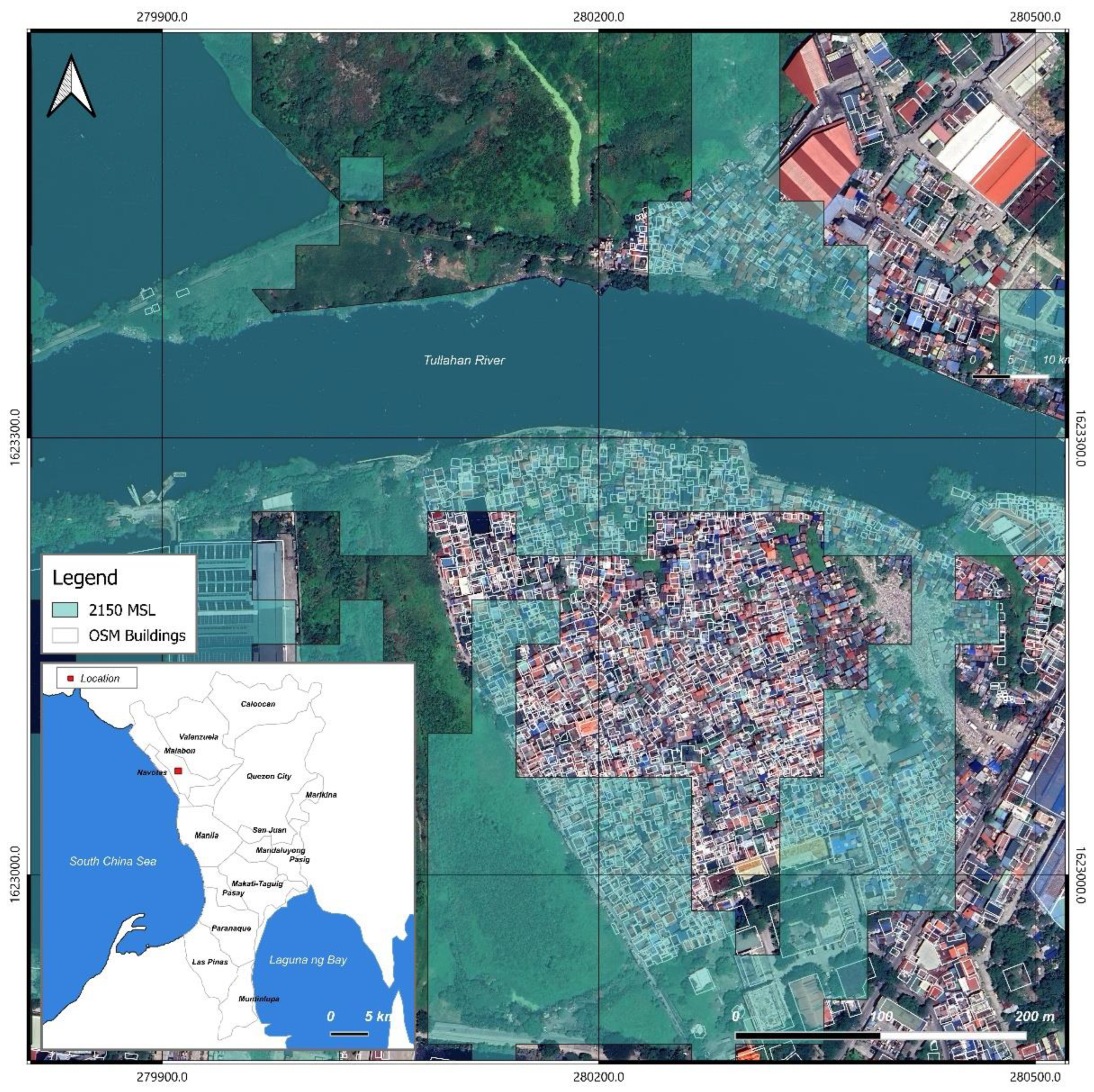
Figure 7.
Permanent flood zone (2150, SSP5-8.5) near the Port of Manila. Inset: location within Metro Manila.
Figure 7.
Permanent flood zone (2150, SSP5-8.5) near the Port of Manila. Inset: location within Metro Manila.
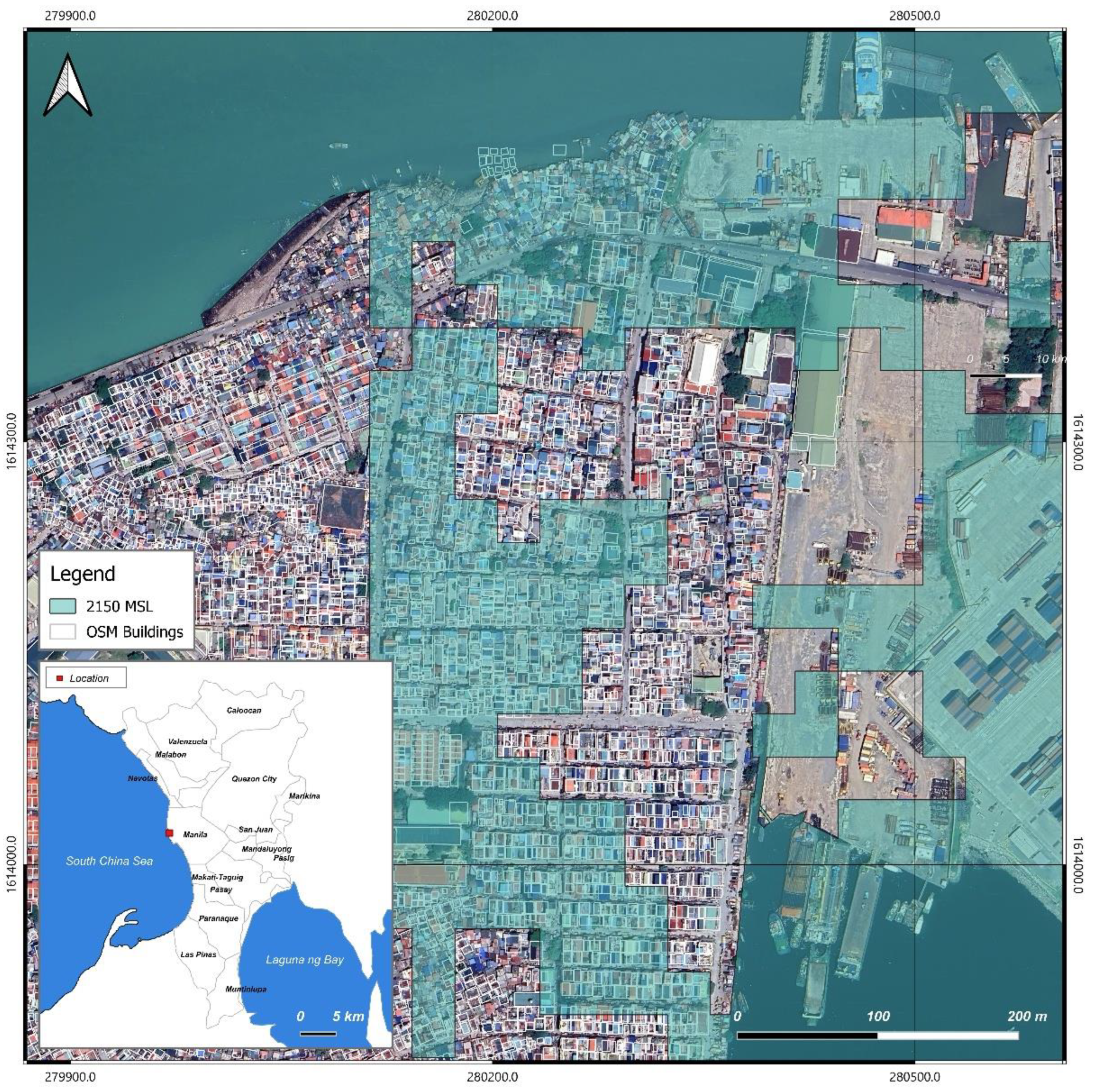

Table 1.
Relative sea level (RSL) projections for the Port of Manila by 2100. GMSL: global mean sea level rise (IPCC AR6, likely range p17–p83). Fr: regional amplification factor by gravitational fingerprints (global range 0.10–0.20, differentiated by SSP). VLM: accumulated vertical land motion (10.1 mm/year × 78 years = 0.785 m). RSL = GMSL × (1 + Fr) + VLM.
Table 1.
Relative sea level (RSL) projections for the Port of Manila by 2100. GMSL: global mean sea level rise (IPCC AR6, likely range p17–p83). Fr: regional amplification factor by gravitational fingerprints (global range 0.10–0.20, differentiated by SSP). VLM: accumulated vertical land motion (10.1 mm/year × 78 years = 0.785 m). RSL = GMSL × (1 + Fr) + VLM.
| Scenario | GMSL (IPCC) [m] | Fr | Local GMSL [m] | VLM accum. [m] | Total RSL [m] |
| SSP1-2.6 | 0.28–0.55 | 1.10–1.15 | 0.31–0.63 | 0.785 | 1.09–1.42 |
| SSP2-4.5 | 0.44–0.76 | 1.12–1.17 | 0.49–0.89 | 0.785 | 1.28–1.67 |
| SSP5-8.5 | 0.63–1.01 | 1.15–1.20 | 0.72–1.21 | 0.785 | 1.51–2.00 |
Table 2.
Relative sea level (RSL) projections for the Port of Manila in 2150. Only SSP1-2.6 and SSP5-8.5 had AR6 projections for 2150. VLM accumulated: 10.1 mm/year × 128 years = 1.289 m.
Table 2.
Relative sea level (RSL) projections for the Port of Manila in 2150. Only SSP1-2.6 and SSP5-8.5 had AR6 projections for 2150. VLM accumulated: 10.1 mm/year × 128 years = 1.289 m.
| Scenario | GMSL (IPCC) [m] | Fr | Local GMSL [m] | VLM accum. [m] | Total RSL [m] |
| SSP1-2.6 | 0.37–0.86 | 1.10–1.15 | 0.41–0.99 | 1.289 | 1.70–2.28 |
| SSP5-8.5 | 0.98–1.88 | 1.15–1.20 | 1.13–2.26 | 1.289 | 2.41–3.54 |
Table 3.
Subsidence sensitivity scenarios.
| Scenario | Description | Rate (mm/yr) | Justification |
| S1: Constant | Mean observed rate 2015–2023 | 10.1 | Baseline, “no intervention” |
| S2: Reduction | Mitigation through groundwater regulation | 5.03 (50% red.) | Sustainable management |
| S3: High | Continuation of accelerated trend | 15.1 | Current max. rates (Sulapas et al., 2024) |
Table 4.
Permanent flood surface by municipality (SSP5-8.5, ocean_flood = 1, excluding current open water).
Table 4.
Permanent flood surface by municipality (SSP5-8.5, ocean_flood = 1, excluding current open water).
| Municipality | 2100 (km²) | % mun. | 2150 (km²) | % mun. | Δ (km²) | Δ (%) | Pop. (2024) |
| Malabon | 2.75 | 10.6 | 4.69 | 18.1 | +1.94 | +71 | 389,929 |
| Manila | 2.63 | 5.8 | 3.16 | 7.0 | +0.53 | +20 | 1,902,590 |
| Navotas | 1.39 | 17.2 | 1.61 | 19.9 | +0.22 | +16 | 252,878 |
| Las Piñas | 0.81 | 1.9 | 1.17 | 2.8 | +0.36 | +44 | 615,549 |
| Parañaque | 0.37 | 0.8 | 0.52 | 1.2 | +0.15 | +41 | 703,245 |
| Total | 7.95 | — | 11.15 | — | +3.20 | +40 | 3,864,191 |
Table 5.
Flooded buildings by municipality (2100 scenario, class 1, ≤ 1.74 m).
| Municipality | No. buildings | Total surface (m²) | Surface (ha) | Predominant type |
| Malabon | 483 | 76,984 | 7.70 | apartments |
| Manila | 460 | 241,272 | 24.13 | service/public |
| Navotas | 207 | 81,038 | 8.10 | residential |
| Las Piñas | 54 | 8,628 | 0.86 | house/industrial |
| Parañaque | 35 | 9,012 | 0.90 | public/retail |
| Makati-Taguig | 1 | 72 | 0.01 | — |
| Pasay | 1 | 44 | 0.00 | house |
| Total | 1,241 | 417,050 | 41.70 |
Table 6.
Natural areas flooded by municipality and type (2100 scenario, class 1).
| Municipality | Type | No. features | Area (m²) | Area (ha) |
| Navotas | Water body | 3 | 643,050 | 64.31 |
| Malabon | Water body | 3 | 406,025 | 40.60 |
| Las Piñas | Water body | 6 | 49,604 | 4.96 |
| Manila | Park | 7 | 53,772 | 5.38 |
| Manila | Water body | 6 | 43,310 | 4.33 |
| Manila | Forest/mangrove | 4 | 36,413 | 3.64 |
| Las Piñas | Forest/mangrove | 1 | 16,740 | 1.67 |
| Parañaque | Park | 2 | 3,998 | 0.40 |
| Total | — | 32 | 1,252,912 | 125.29 |
Table 7.
Flooded linear infrastructure by municipality: comparison 2100 vs. 2150 (SSP5-8.5).
| Municipality | 2100 (km) | 2150 (km) | Δ (%) | Roads (km) | Waterways (km) | Railway (km) | No. segments 2150 |
| Manila | 44.38 | 53.65 | +21% | 43.73 | 8.84 | 1.08 | 767 |
| Malabon | 29.86 | 42.17 | +41% | 19.79 | 22.38 | — | 222 |
| Parañaque | 9.92 | 14.74 | +49% | 12.37 | 0.72 | 1.65 | 241 |
| Las Piñas | 11.94 | 16.97 | +42% | 12.60 | 2.33 | 2.04 | 199 |
| Navotas | 10.03 | 11.65 | +16% | 8.90 | 2.75 | — | 130 |
| Total | 106.14 | 139.18 | +31% | 97.39 | 37.02 | 4.77 | 1,559 |
Disclaimer/Publisher’s Note: The statements, opinions and data contained in all publications are solely those of the individual author(s) and contributor(s) and not of MDPI and/or the editor(s). MDPI and/or the editor(s) disclaim responsibility for any injury to people or property resulting from any ideas, methods, instructions or products referred to in the content. |
© 2026 by the authors. Licensee MDPI, Basel, Switzerland. This article is an open access article distributed under the terms and conditions of the Creative Commons Attribution (CC BY) license (http://creativecommons.org/licenses/by/4.0/).
Copyright: This open access article is published under a Creative Commons CC BY 4.0 license, which permit the free download, distribution, and reuse, provided that the author and preprint are cited in any reuse.


