

Submitted:
25 February 2026
Posted:
02 March 2026
Read the latest preprint version here
Abstract
Background: many wildfire models simulate fire spread by resolving the front-normal velocity (spread rate) as a function of the local environmental conditions and the orientation of the fire front. We study one such model, here called the wind-projected Rothermel model, which extends the Rothermel model to all front orientations by using the front-normal component of the midflame wind speed \( \vec{U} \): \( R(\vec{n}) = R_0 (1 + A \max(0, \vec{n} \cdot \vec{U})^B) \) Methods: we apply the mathematical methods recently developed by the authors to solve front propagation in spatially constant conditions. Results: as soon as wind is moderately high, the model undergoes heading fire collapse, i.e. the downwind-facing front collapses to a pointed shape, which then advances at a lower speed than predicted by the Rothermel model. Formulas are derived to compute the characteristic length and time scales of the collapse. The effect is more pronounced for finer fuels that have a higher wind exponent. Conclusions: the formulas provided here can facilitate model validation. Heading fire collapse is frequent in this model; this is a salient point for model validation, as it makes the model behavior drastically different from other Rothermel extensions, like those based on elliptical Huygens wavelets. This also threatens the validity of some numerical implementations.
Keywords:
wildland fire
; fire behavior model
; model verification
; rothermel model
1. Introduction
Fire spread models are mathematical models and numerical algorithms that aim to simulate the propagation and behavior of wildland fire fronts. Many fire spread models propagate the fire front by resolving the front-normal velocity (rate of spread) as a function of:
- 1.
- the local environmental conditions (fuel type, wind, terrain), and
- 2.
- the unit vector normal to the fire front.
The idea of the dependency on is that there is some direction, which we call the heading fire direction, in which the fire front advances fastest (typically, on flat terrain, the heading fire direction is the downwind direction).
In [1], the authors have called these speed-from-tangent models, and derived exact analytical formulas that calculate the evolution of the fire front under spatially constant conditions, provided that the initial fire front delineates a convex region. In the context of the Level-Set Method [2] and its Hamilton-Jacobi equation, these formulas yield the same fire progressions as the Hopf Formula [3,4], when applicable. These formulas are generally useful for understanding some implications of the fire spread model, and also for validating the precision of numerical simulation algorithms.
Furthermore, [1] has also shown that under certain conditions, the model will yield what we call heading fire collapse, where the heading fire front advances so fast compared to other front orientations that it collapses into a sharp pointed shape. After the collapse, the tip of the point advances more slowly than the heading fire spread rate one would intuitively expect. [1] shows that heading fire collapse occurs when the heading fire direction is sheltered by a concavity in the polar plot of , in which is the front-normal spread rate expressed as a function of an angle representing the front-normal azimuth. The existence of such a concavity is equivalent to the Hamiltonian being non-convex in the corresponding Hamilton-Jacobi equation, whereas a convex Hamiltonian corresponds to following Huygens’ Principle. Post-collapse, the asymptotic shape and speed of the point correspond to filling the concavity of said polar plot.
This paper applies the methods of [1] to study a particular case of speed-from-tangent model, which we will call the projected-wind Rothermel model, in which the front-normal spread rate is given by an equation of the form:
in which is the midflame wind speed vector, is the elevation gradient, is the no-wind no-slope spread rate, and are positive constants determined by the fuel type using Rothermel equations [5]. The Rothermel model [5] only calculates the spread rate in the heading fire direction when the upslope and downwind direction are aligned; the above equation provides an intuitive extension of the Rothermel model that calculates fire spread in all directions, through the use of dot products. The authors have encountered this model in the context of the WRF-Fire model [6]. This model was introduced by [7]; [8] recently proposed a high-resolution numerical scheme for implementing it.
This paper will study the conditions under which heading fire collapse occurs in the above model. For simplicity, we will restrict our attention to the case of flat terrain, i.e. . We will see that heading fire collapse occurs whenever the midflame wind speed U exceeds a critical threshold , which is quite low for most fuel types. We will also compute the asymptotic shape and speed of the post-collapse pointed fire front.
Without further ado, let us visualize how our model behaves. Figure 1 shows the evolution of the fire front over time, from an initial fire ignited as a line segment perpendicular to the wind direction. This fire progression was obtained not by simulation, but by direct application of the analytical formulas derived in [1]. We observe what [1] described as heading fire collapse: the heading fire starts by advancing in the downwind direction at the velocity predicted by Rothermel equations [5], becoming progressively narrower until it collapses into a pointed shape. Importantly, after the collapse, the fire advances more slowly in the downwind direction. We note that the observed fire shape is in qualitative agreement with the one obtained through simulations in [8].
Figure 1 has shown us one combination of fuel type and weather conditions that leads to heading fire collapse in the projected-wind Rothermel model (we used the same combination of wind speed, fuel type and non-wind-no-slope spread rate as in [6], yielding m/s, m/s, , m/s; a point of disagreement is that we obtained a slightly higher heading spread rate m/s, which drives us to question the calculations in [6]). So far, this is an anecdotal, qualitative finding, which naturally motivates us to study the phenomenon more systematically and quantitatively:
- 1.
- How often does heading fire collapse occur in the projected-wind Rothermel model? In other words, under what conditions does heading fire collapse occur? This is answered by Theorem 1.
- 2.
- What are the characteristic length and time scales of the collapse? This is answered by Theorem 2 and Equation 27.
- 3.
- How much slower is the forward fire spread after the collapse? This is answered by Theorem 1 and Equation 16.
This paper is organized as follows. Section 2.1 recalls the Rothermel model, and in particular its formula for the effect of wind speed on heading spread rate (Section 2.1.1), as well as how model parameters are derived from fuel characteristics (Section 2.1.2). Then, Section 2.2 recalls how the projected-wind Rothermel model extends the classical Rothermel model to all front orientations. Now the paper starts making original contributions: Section 2.3 uses the methods of [1] to solve fire spread from a point ignition, revealing that the model experiences heading fire collapse whenever the midflame wind speed exceeds a (relative low) threshold , and computes the asymptotic post-collapse velocity through what we call the asymptotic slowdown ratio - see Theorem 1. Then, Section 2.4 studies fire spread from a wind-perpendicular line segment, similarly to [6]: Section 2.4.1 specializes the formulas of [1] to calculate the analytical solution and produce Figure 1, which enables Section 2.4.2 to describe the length and time scales of the collapse, by computing what we call the distance-to-collapse and the time-to-collapse. Section 2.5 provides the mathematical proofs. Finally, Section 3 applies the above results to the concrete fuel models from [9].
No fire spread simulations are done in this analysis - all computations are based on exact mathematical formulas.
2. Materials and Methods
This section conducts the mathematical analysis from which the findings of this paper are derived. The main symbols and notation are summarized in Table 1.
2.1. The Classical Rothermel Model
This section introduces the classical Rothermel model [5], which predicts the velocity of the fire front only in the heading fire direction, i.e. the direction of maximum spread rate. The projected-wind Rothermel model that the present paper studies is an extension of the classical Rothermel model that predicts the velocity of the fire front in all directions.
2.1.1. Wind and Slope Dependency
The Rothermel model [5] calculates the heading fire spread rate (in m/s) as:
in which:
- 1.
- is the no-wind no-slope spread rate (m/s),
- 2.
- is the wind factor (unitless, typical range 0-100), and
- 3.
- is the slope factor (unitless, typical range 0-50).
Keep in mind that is the spread rate only in the heading fire direction, which is the downwind direction on flat terrain.
Most of the sophistication in the Rothermel model goes into calculating , which is a function of fuel type and fuel moisture variables, and will be largely irrelevant to the our analysis. The factor accounts for the effect of slope; we will disregard it because it is not our interest here.
The factor captures the fact that higher wind speeds cause fires to spread faster, and is calculated as a function of the midflame wind speed U. is traditionally expressed as the power law , which we find more insightful to rewrite as:
in which and B are positive constants that depend on the fuel model, with the following interpretation:
- 1.
- means that . Thus, is the midflame wind speed which causes a doubling in spread rate compared to a no-wind situation. typically ranges from 0.1 to 0.6 m/s.
- 2.
- B is the wind exponent, typically ranging from 1.1 to 1.5. B can be viewed as the elasticity of spread rate with respect to wind speed: a 1% increase in U leads to a B% increase in . If , then .
Thus, for a given midflame wind speed U, is a decreasing function of .
2.1.2. Fuel Model Dependency
This section recalls how the parameters and B are computed in the Rothermel model; it is included for context and reproducibility, and may safely be skipped by readers uninterested in those details.
and B are fully determined by the fuel model, regardless of weather conditions. More precisely, and B are fully determined by 2 quantities:
- 1.
- The Surface-Area to Volume (SAV) ration (typical range: 3,000 to 12,000 ), which quantifies fuel fineness.
- 2.
- The Relative Packing Ratio (unitless, typical range 0.15 to 6.5) which quantifies the compactness of the fuel bed (highest for litter, lowest for grass), and therefore the resistance to convective heat transfer.
See Figure 2 to visualize the variation of and B with and , along with the values taken for the Anderson and Scott & Burgan fuel model classifications [9]. Some comments:
- 1.
- B is an increasing function of , capturing the fact that finer fuels respond more "explosively" to increases in wind speed.
- 2.
- increases with : more compact fuel beds lead to smaller spread rates.
- 3.
- also increases with : for finer fuels, it takes a higher wind speed to start seeing a significant effect on spread rates.
Warning: U is the midflame wind speed, and is therefore different and lower than the 10m wind speed typically provided in weather datasets. A difficulty with the Rothermel model is that U is not a precisely defined quantity: fire behavior models typically compute it by discounting 10m wind speed by some factor that accounts for surface roughness.
As a sanity check, we computed fuel properties using the above formulas, for a sample of fuel models. The results are displayed in Table 2. This computes the same information as table 22 of [5]; skeptical readers are encouraged to compare both tables and verify that they contain the same values, which suggests that our calculations are error-free.
2.2. The Projected-Wind Rothermel Model
We now introduce what we call the projectd-wind Rothermel model, which is the object of the present study.
In order to generalize the classical Rothermel model (equation 2) to all orientations of the fire front, the projected-wind Rothermel model simply replaces the wind speed U by its front-normal component (or zero if the wind blows into the fire front). With our simplifying assumption that there is no slope, this yields:
We denote the angle between the front-normal direction and the heading fire direction (downwind), so that . Recalling that is the Rothermel wind factor , we can rewrite equation 8 as a function of :
Without loss of generality, we will study the normalized spread rate , which is the spread rate in the direction divided by the no-wind no-slope spread rate . We can therefore express as:
Thus is maximal at (the downwind direction), with value .
2.3. Conditions for Heading Fire Collapse
Having set the background, we now study in which conditions heading fire collapse occurs. We know from [1] that heading fire occurs when the polar plot of the inverse spread rate profile is non-convex, more precisely when the heading fire direction is sheltered by a concavity.
To make things concrete, let us visualize such polar plots on a few examples. Figure 3 shows the fire shape and inverse spread rate profile for various combinations of B, , and U. B and are chosen to be typical fuel values. The fire shape (in m/s) corresponds to letting the fire grow from a point ignition at the origin for a unit duration; it is computed using the methods in [1], that is by computing what the authors called the polar Legendre-Fenchel transform of the inverse spread rate profile i.e.:
To express this in more standard mathematical terminology from convex analysis [10] and Hamilton-Jacobi theory [4], the indicator function of the asymptotic fire shape is the convex conjugate of the system’s Hamiltonian (this is shown in [1]).
To be clear, is the correct fire shape that follows from the model when spreading from a point ignition under constant conditions (a key result of [1] is that this shape can be calculated analytically, using what the authors called the polar Hopf Formula.) It might seem contrived to use a point ignition instead of a larger initial perimeter, but note that is also the asymptotic fire shape when the fire front becomes much larger than the initial perimeter.
As explained in [1], several qualitative aspects of the fire shape can be predicted by examining the polar plot of . For example, has sharp corners at , which translate into straight line segments at the flanks of the fire perimeter. Furthermore, for high enough wind speeds, has a concavity sheltering (semitransparent green shading), which translates into a sharp pointed shape at the head of the fire (what we have been calling heading fire collapse), so that the fire front is shaped like a bullet. When that happens, we have : the fire front falls short of advancing at the heading spread rate, because of heading fire collapse.
The asymptotic slowdown ratio is of interest, because it quantifies how much asymptotically slower the fire advances compared to the Rothermel-predicted heading spread rate . Because corresponds to “filling” (by convex extrapolation) the concavity that shelters the heading fire direction, it is readily verified that this ratio can be expressed using the angle defined as the half-angle of this concavity:
We are now ready to characterize the conditions for heading fire collapse:
Theorem 1
(Wind speed threshold for Heading Fire Collapse). We assume σ is high enough that .
Heading fire collapse occurs if and only if , in which is a critical wind speed defined as:
This is equivalent to , in which is thecritical wind factordefined as:
Then, has a concavity sheltering , and the half-width of this concavity is given by the angle defined as:
Furthermore, the asymptotic slowdown ratio can be calculated as:
See Section 2.5 for a proof of Theorem 1. Note that Equation 15 is how we computed the angular ranges of concavities in Figure 3. Therefore, Figure 3 provides visual confirmation that Equation 15 is correct.
Also note that provided two equivalent formulations of the wind speed threshold: and . The equivalence between both formulations is made clearer by observing that:
Figure 4 shows how the asymptotic slowdown ratio varies with the wind factor . We see that the slowdown effect becomes stronger with higher wind factor (and therefore, higher wind speed), and also with higher wind exponent B.
2.4. Fire Growth from a Wind-Perpendicular Line Segment Ignition
The previous section only described asymptotic fire growth, or said equivalently, fire growth from a point ignition, which does not let us observe heading fire collapse (collapse is instantaneous when starting from a point ignition). Therefore, to derive the quantitative characteristics of heading fire collapse in our model, we will study fire growth not from a point ignition, but from an initial burned region which is a line segment perpendicular to the wind direction, as shown in Figure 1. Note that this is the same configuration as in [6].
We will call the initial line segment, and its half-length. We will use Cartesian coordinates , in which:
- the origin is at the midpoint of the initial line segment,
- the x-axis points downwind,
- the y-axis is perpendicular to the wind direction.
2.4.1. Solving for the Time-of-Arrival Function
We will first derive the exact expression for the fire spread, based on the formulas in [1]. We denote the time-of-arrival function, which describes the time since ignition at which the fire front reaches the location given by vector . Recall from [1] that the time-of-arrival function is given by:
in which denotes an inverse velocity vector, is the Hamiltonian of the system, and each is the time-of-arrival function of an infinite linear fire front advancing at inverse-velocity that has just burned past the initial perimeter at time :
in which is the indicator function of , and is its convex conjugate (see Appendix A), and therefore:
Let us specialize these formulas to our problem. Equation 20 maximizes a convex function over a convex polytope (the line segment ), and therefore the sup can be taken over the end points of the segment:
Furthermore, the sup in equation 18 can be taken over vectors such that , i.e. those that saturate the constraint . We parameterize them by polar coordinates: denoting the unit vector in direction , we define an inverse-velocity vector as:
This yields a new expression for the time-of-arrival function:
2.4.2. Quantifying Heading Fire Collapse
We are now ready to compute the quantitative characteristics of heading fire collapse: distance to collapse and time to collapse . What we call the distance to collapse corresponds to the x-axis coordinate where the tip of the point forms, i.e. where the heading fire direction () is no longer represented by the fire front. The time-to-collapse is simply the time at which that happens, i.e. the time of arrival at that location.
Theorem 2
(Distance-to-collapse from a cross-wind line segment). We assume and , so that the conditions for heading fire collapse are met.
We denote the helper function defined as:
Then, the distance to collapse is given by:
See Section 2.5 for a proof of Theorem 3. Note that the time-to-collapse can be calculated as , and therefore:
It is worth noting that the distance-to-collapse is independent of the no-wind-no-slope spread rate , thus factoring out much of the complexity of the Rothermel model.
Furthermore, when wind speed becomes high , the distance-to-collapse decreases to an asymptotic value that depends only on the wind exponent B:
Theorem 3
(High-wind asymptotics for distance-to-collapse).
This result is illustrated by Figure 5.
Theorem 3 is remarkably counter-intuitive: one might generally expect that higher wind speeds would cause more elongated fire shapes, yet the math shows that the opposite is happening: at higher wind speeds, heading fire collapse will happen sooner in time, but at shorter distances from the initial fire line.
2.5. Mathematical Proofs
This section proves the theorems stated in previous sections. The required background consists of the concepts from [1], along with basic univariate calculus and plane geometry.
Proof
(Proof of Theorem 1). In the polar plot of , the heading fire direction is sheltered by a concavity if and only if
for some . (To see it, note that is the x-axis coordinate of the curve at angle .) The above equation is equivalent to:
or, substituting the expression for , and simplifying:
Using the change of variable , we will therefore seek to find the value that minimizes the function:
for , then confirm that . Observe first that , and as .
Differentiating f, we get:
Setting , we get:
Thus, having a soluion implies that:
which requires that , i.e. as stated in the theorem. When that holds,
is indeed the unique minimum of on , because for and for . In particular, , as required.
Note that by definition of , ; this shows that is equivalent to .
All that remains to do is to calculate the asymptotic slowdown ratio . Observe that by definition of f, this ratio is equal to ; we then substitute and to get
which simplifies into equation 16. This completes the proof. □
Proof
(Proof of Theorem 2). Recall from Section 2.4.1 and [1] that the burned region at time t can be described as an intersection of half-planes, each delimited by an infinite “fire line” that advances at the spread rate predicted by the model; Equation 23 describes this interpretation in terms of time-of-arrival functions.
Denote the position on the x axis of the -oriented fire line at time t. By applying Equation 24 to solve for x, it is easily verified that can be expressed as:
Heading fire collapse occurs when the line corresponding to “escapes” from the region delineated by the other lines. Therefore, heading fire collapse has happened when
for some t and some . When that’s the case, and . In what follows, we will essentially be looking for the “smallest” , i.e. the that gets overcome first by the heading fire line at .
Substituting the expressions for and , we get:
Substituting (which implies ) and re-arranging, we obtain:
and finally:
It follows from the above that
We recognize the expression inside the inf in the definiton of in Equation 25. We further need to show that the infimum cannot be achieved for any . Indeed, if , denoting , there is always another with that achieves an x-axis velocity , but with a lower starting position , proving that .
3. Results
We applied Theorem 1 to the Rothermel fuel equations, i.e. to how the Rothermel model [5] predicts the model parameters and B (see Section 2.1.2). We computed the critical wind speed and the critical wind factor (see Theorem 1) for a typical range of fuel characteristics, as captured by the SAV ratio and the relative packing ratio . We also computed the high-wind asymptotic distance-to-collapse (equation 28). The results are plotted in Figure 6.
Figure 6 shows that heading fire collapse is not a rare phenomenon: it occurs whenever the wind has a moderate to strong influence, since we will have for most fuel types.
4. Discussion
This paper has demonstrated a strong prevalence of heading fire collapse in the projected-wind Rothermel model. Arguably, this has significant consequences.
To many users, the projected-wind Rothermel model might seem like an innocuous choice - one of many similar parameterizations of fire front kinetics that are consistent with Rothermel-predicted heading fire velocities. However, based on the above analysis, we argue that the projected-wind Rothermel model is drastically different from other Rothermel extensions like those FARSITE and Prometheus [11,12], which are based on ellipical Huygens wavelets. Indeed, Huygens wavelet models follow Huygens’ Principle, and therefore preserve the smoothness of the fire front [1] and advance at the Rothermel-predicted heading spread rate, whereas the projected-wind Rothermel model does not follow the Huygens principle, and is subject to heading fire collapse as shown in this paper. Therefore, we argue that it makes a critical difference to choose one approach or the other.
By the way, in our opinion, these findings put into question some of the conclusions of [6], namely that the new numerical methods adopted in [6] reduced the numerical error in their uniform velocity field experiment. From what we understand, [6] saw it as an improvement that the fire front took less of a “bow” shape and more of a rectangular shape. However, our results have now revealed that the original bow shape was closer to the theoretical solution than the rectangular shape expected in [6]. We suspect that the authors of [6] expected a roughly rectangular shape because they were essentially assuming that Huygens’ Principle would apply (i.e. that the final burned region could be obtained by applying a convolution of the initial burned region and some elongated shape); however, as shown in [1], the Huygens principle cannot apply when the Hamiltonian is non-convex.
In contrast, the fire shapes obtained by simulation in [8] seem to agree with the analytical solutions derived in the present paper. The analysis of [8] might improved by using this analytical solution as their reference, instead of relying on higher-resolution simulations.
As discussed in [1], heading fire collapse might be a real phenomenon. However, we have reasons to be wary of its prevalence in the model here studied. If we assume that heading fire collapse is an unrealistic model artifact, its occurrence in models leads to the following biases:
- 1.
- Underprediction of fire front velocity (the heading fire falls short of being simulated to its full speed, as we saw.)
- 2.
- Underprediction of fire line intensity, because fire intensity is typically computed from the front-normal spread rate, and heading fire collapse causes high-spread-rate front orientations to be unsustainable.
- 3.
- Therefore, underprediction of firefighting difficulty and ecological severity, as that’s typically derived from fire line intensity.
As mentioned in [1], pointed shapes can develop (in real or simulated fires) as a consequence of fire-atmosphere feedbacks; however, this is definitely not what is happening in the present paper. The pointed shapes we see are not a consequence of fire-atmosphere coupling: indeed, we have worked under the hypothesis of spatially constant wind inputs, which means that fire-atmosphere coupling is effectively turned off. The pointed shapes we see in this paper are purely a consequence of non-convex frontal kinetics, and the heading fire collapse mechanism we have described.
We humble admit that we do not know why the projected-wind Rothermel model is so popular among coupled fire-atmosphere models, as mentioned in [6]. It might be for good scientific reasons, i.e. that model authors have got evidence that it is realistic - the present paper does not claim to settle this question. However, it might also be adopted for bad reasons, e.g. because model authors find it to be a low-effort generalization of the Rothermel model, with a pleasingly simple formula, or because they prefer to focus on other modeling components like atmospheric physics. We encourage model authors to revisit this choice, based on the findings of this paper.
Supplementary Materials
The following supporting information can be downloaded at the website of this paper posted on Preprints.org. File front_propagation.py contains the Python code used to produce the figures in the paper.
Author Contributions
Conceptualization, V.W.; methodology, V.W.; software, V.W.; validation, V.W. and D.S.; formal analysis, V.W.; investigation, V.W.; resources, D.S.; data curation, V.W.; writing—original draft preparation, V.W.; writing—review and editing, V.W. and D.S.; visualization, V.W.; supervision, D.S.; project administration, D.S.; funding acquisition, D.S. All authors have read and agreed to the published version of the manuscript.
Funding
This research received no external funding.
Institutional Review Board Statement
Not applicable.
Informed Consent Statement
Not applicable.
Data Availability Statement
Data is contained within the article or supplementary material - see Python code in file front_propagation.py.
Conflicts of Interest
The authors declare no conflicts of interest.
Appendix A. Convex Analysis Background
We recall some concepts from convex analysis; see [10,13,14] for an introduction to convex analysis. We will use the same notations as in [10]. These concepts are also recalled in [1].
If A is a subset of , the indicator function of A is defined as:
is a convex function if and only if A is a convex set.
If f is a real-valued function of a vector-valued variable, its convex conjugate (also called its Legendre-Fenchel transform or its Fenchel transform), is defined as:
Some properties:
- is a convex function.
- if and only if f is convex.
- is the convex extrapolation of f, i.e. the smallest convex function that is no greater than f.
- if A is a set, then is 1-homogeneous, i.e. for all .
References
- Waeselynck, V.; Saah, D. Pointy-Headed Fires: On the Convex Duality Between Fire Shapes and Spread Rates in Fire Growth Models. Preprints 2026. [Google Scholar] [CrossRef]
- Sethian, J.A. A fast marching level set method for monotonically advancing fronts. proceedings of the National Academy of Sciences 1996, 93, 1591–1595. [Google Scholar] [CrossRef] [PubMed]
- Hopf, E. Generalized solutions of non-linear equations of first order. Journal of Mathematics and Mechanics 1965, 14, 951–973. [Google Scholar]
- Evans, L.C. Envelopes and nonconvex Hamilton–Jacobi equations. Calculus of Variations and Partial Differential Equations 2014, 50, 257–282. [Google Scholar] [CrossRef]
- Andrews, P.L. The Rothermel surface fire spread model and associated developments: a comprehensive explanation; 2018. [Google Scholar]
- Muñoz-Esparza, D.; Kosović, B.; Jiménez, P.A.; Coen, J.L. An accurate fire-spread algorithm in the Weather Research and Forecasting model using the level-set method. Journal of Advances in Modeling Earth Systems 2018, 10, 908–926. [Google Scholar] [CrossRef]
- Mallet, V.; Keyes, D.E.; Fendell, F. Modeling wildland fire propagation with level set methods. Computers & Mathematics with Applications 2009, 57, 1089–1101. [Google Scholar] [CrossRef]
- Mandikas, V.G.; Voulgarakis, A. High-Resolution Numerical Scheme for Simulating Wildland Fire Spread. Mathematics 2025, 13, 3721. [Google Scholar] [CrossRef]
- Scott, J.H.; Burgan, R.E. Standard fire behavior fuel models: a comprehensive set for use with Rothermel’s surface fire spread model. The Bark Beetles, Fuels, and Fire Bibliography 2005, 66. [Google Scholar]
- Tiel, J.v. Convex analysis: an introductory text. No Title 1984. [Google Scholar]
- Finney, M.A. FARSITE, Fire Area Simulator–model development and evaluation; The Station, 2004. [Google Scholar]
- Tymstra, C.; Bryce, R.; Wotton, B.; Taylor, S.; Armitage, O.; et al. Development and structure of Prometheus: the Canadian wildland fire growth simulation model. Natural Resources Canada, Canadian Forest Service, Northern Forestry Centre, Information Report NOR-X-417. (Edmonton, AB) 2010. [Google Scholar]
- Touchette, H. Legendre-Fenchel transforms in a nutshell. 2005, p. 25. Available online: http://www.maths.qmul.ac.uk/ht/archive/lfth2.pdf.
- Rockafellar, R.T. Convex analysis:(pms-28). 2015. [Google Scholar]
Figure 1.
Fire growth in the projected-wind Rothermel model under constant conditions that are conducive to heading fire collapse. The midflame wind blows eastward at speed m/s. The fire is started from a 1km-wide line segment perpendicular to the wind direction, and spreads on horizontal terrain with Anderson fuel model 1 (short grass). Solid black contour lines show the fire front every 5 minutes, computed exactly by the Hopf Formula for time-of-arrival functions. The grey solid line show the front at the time that the heading fire collapses into a pointed shape; the dashed grey lines show the front shortly before and after , thus showing that was computed accurately. The dashed red line marks the distance-to-collapse . and were computed using the model-specific formulas derived in the present paper; their agreement with the contour lines confirms that these formulas are correct.
Figure 1.
Fire growth in the projected-wind Rothermel model under constant conditions that are conducive to heading fire collapse. The midflame wind blows eastward at speed m/s. The fire is started from a 1km-wide line segment perpendicular to the wind direction, and spreads on horizontal terrain with Anderson fuel model 1 (short grass). Solid black contour lines show the fire front every 5 minutes, computed exactly by the Hopf Formula for time-of-arrival functions. The grey solid line show the front at the time that the heading fire collapses into a pointed shape; the dashed grey lines show the front shortly before and after , thus showing that was computed accurately. The dashed red line marks the distance-to-collapse . and were computed using the model-specific formulas derived in the present paper; their agreement with the contour lines confirms that these formulas are correct.
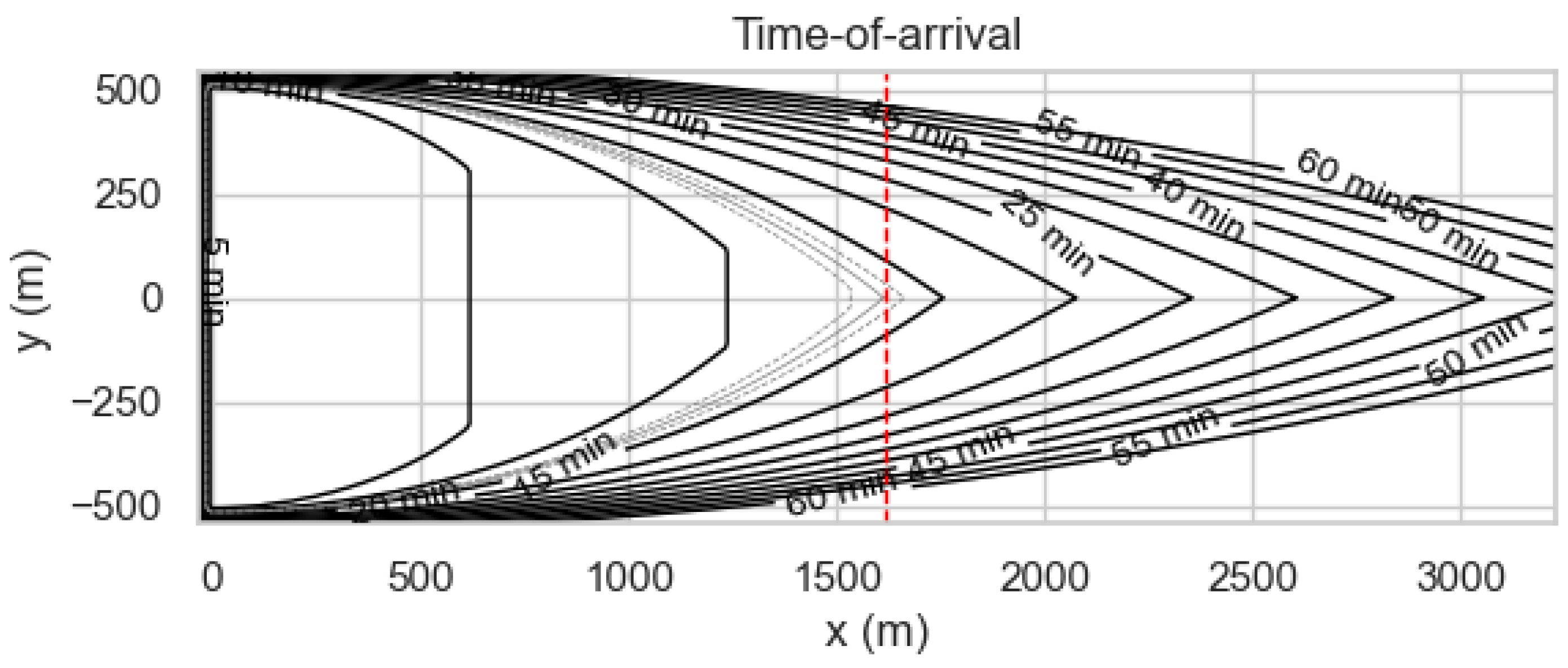
Figure 2.
Wind dependencies in the classical Rothermel model (, ). The top graph plots the wind exponent B: higher values mean a more superlinear response to increases in wind speed. Black contours in the bottom graph show , the midflame wind speed where , i.e. that doubles the heading fire spread rate compared to the no-wind no-slope case. The 53 Scott & Burgan fuel models are displayed as colored numbers; the Anderson fuel types are prefixed with ’A’. The x-axis is the Surface-Area to Volume (SAV) ratio (higher for finer fuels). The bottom y-axis (log scale) shows the relative packing ratio , quantifying fuel bed compactness (higher means more resistance to convective heat transfer).
Figure 2.
Wind dependencies in the classical Rothermel model (, ). The top graph plots the wind exponent B: higher values mean a more superlinear response to increases in wind speed. Black contours in the bottom graph show , the midflame wind speed where , i.e. that doubles the heading fire spread rate compared to the no-wind no-slope case. The 53 Scott & Burgan fuel models are displayed as colored numbers; the Anderson fuel types are prefixed with ’A’. The x-axis is the Surface-Area to Volume (SAV) ratio (higher for finer fuels). The bottom y-axis (log scale) shows the relative packing ratio , quantifying fuel bed compactness (higher means more resistance to convective heat transfer).
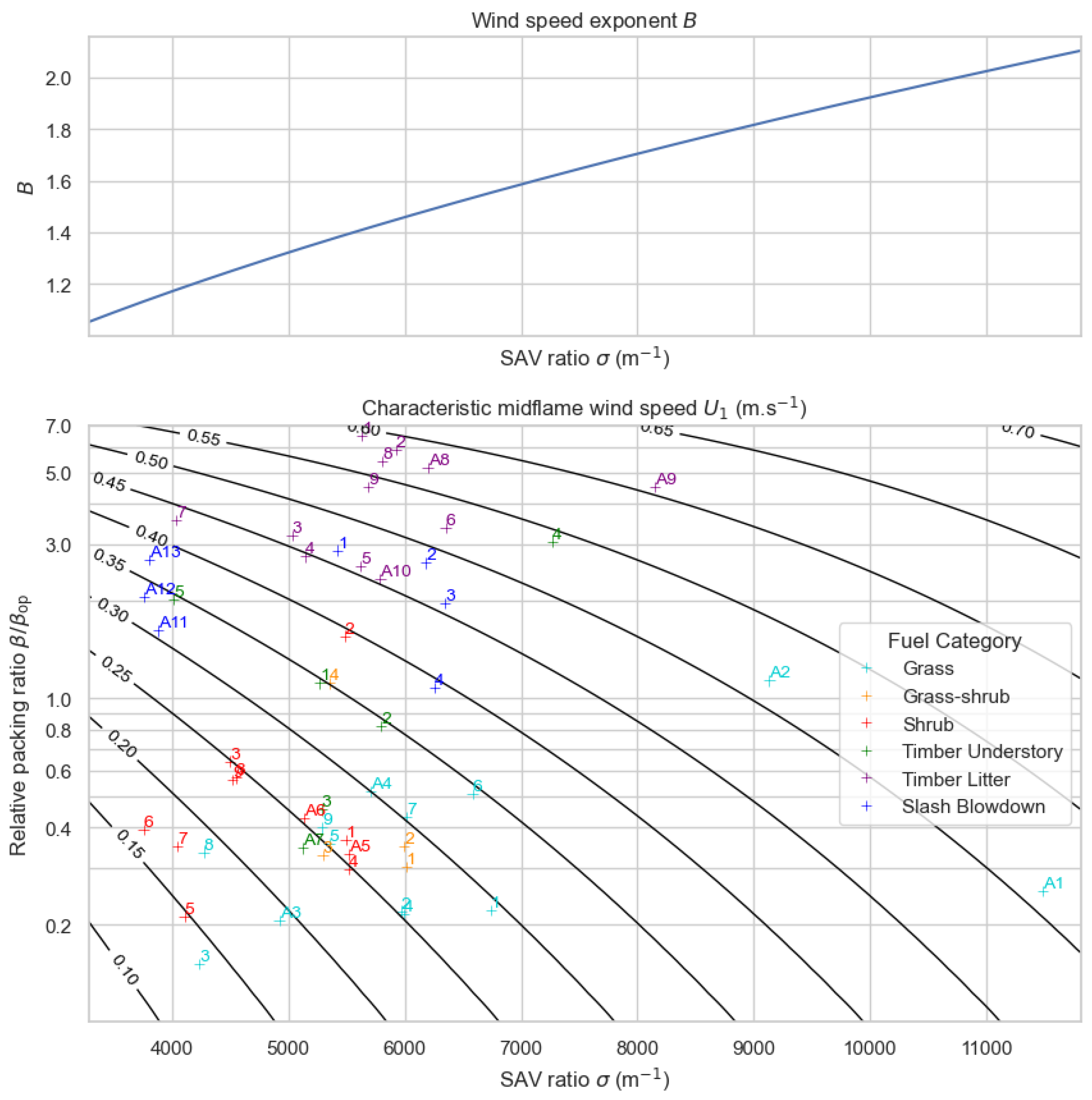
Figure 3.
Asymptotic fire shapes and inverse spread rate profiles in the projected-wind Rothermel model, for a fuel model with wind speed exponent and characteristic wind speed , at various midflame wind speeds: (a) , (b) , (c) , (d) . Heading fire collapse will occur whenever the heading direction is sheltered by a concavity. Such concavities are highlighted in semitransparent green. The half-angle of these concavities is denoted ; front-normal directions are unsustainable and therefore not represented in the fire shapes, making them pointed. It is shown in this paper that such concavities exist whenever U exceeds a threshold which can be expressed from and B, or equivalently when exceeds a critical threshold .
Figure 3.
Asymptotic fire shapes and inverse spread rate profiles in the projected-wind Rothermel model, for a fuel model with wind speed exponent and characteristic wind speed , at various midflame wind speeds: (a) , (b) , (c) , (d) . Heading fire collapse will occur whenever the heading direction is sheltered by a concavity. Such concavities are highlighted in semitransparent green. The half-angle of these concavities is denoted ; front-normal directions are unsustainable and therefore not represented in the fire shapes, making them pointed. It is shown in this paper that such concavities exist whenever U exceeds a threshold which can be expressed from and B, or equivalently when exceeds a critical threshold .
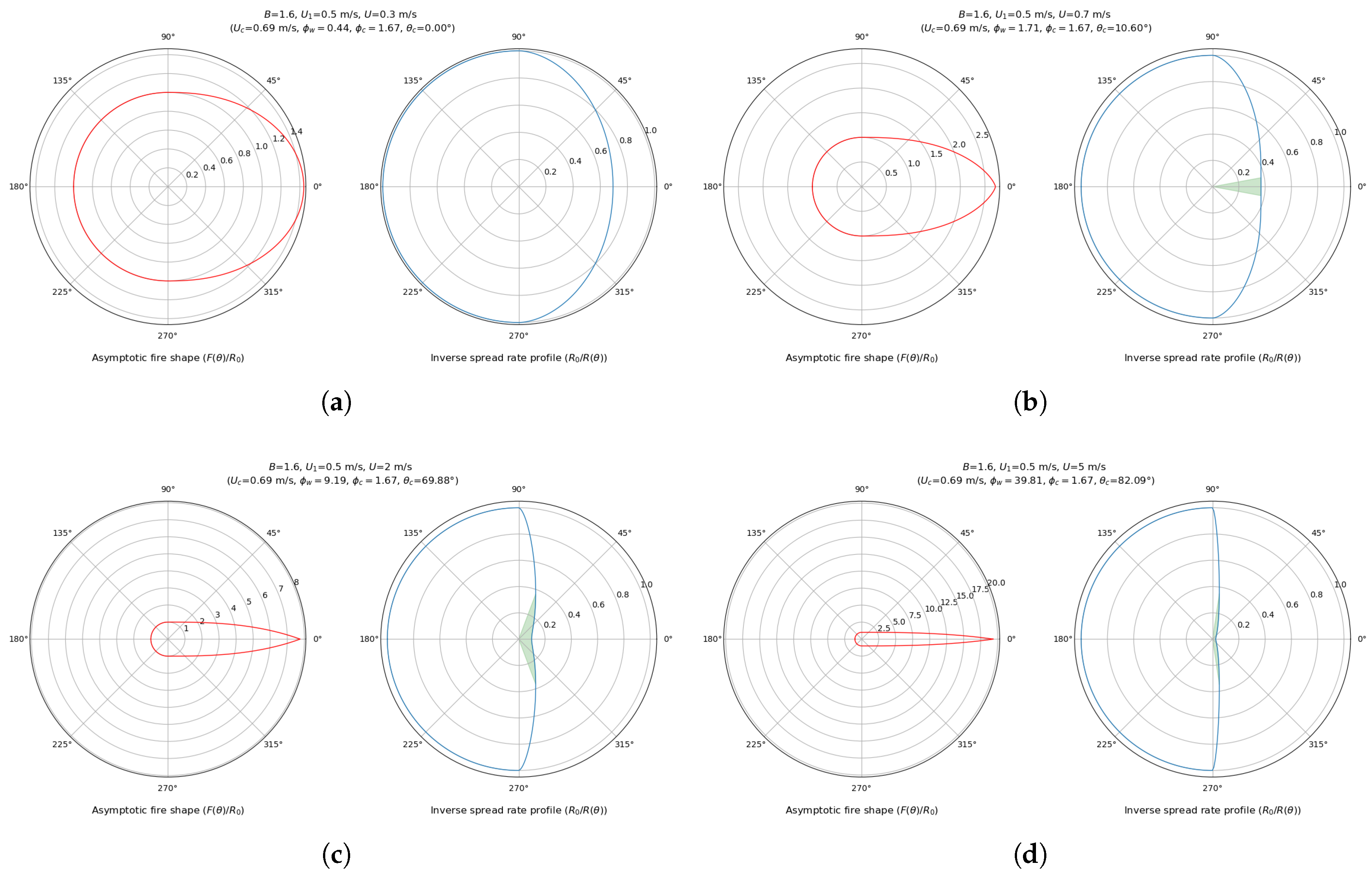
Figure 4.
Asymptotic slowdown ratio as a function of the wind factor and the wind exponent B.
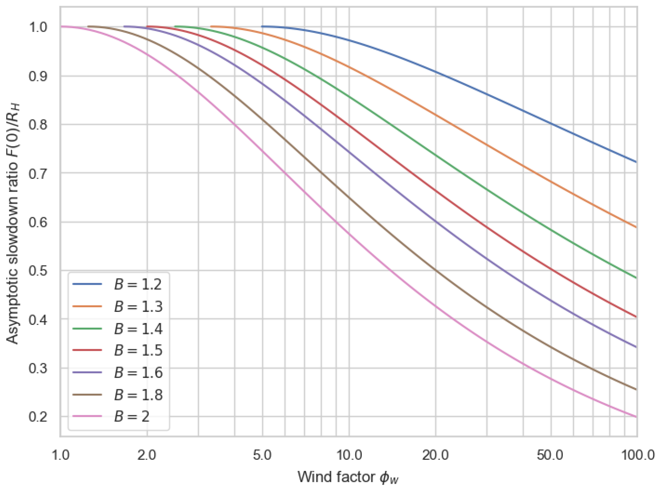
Figure 5.
Distance-to-collapse as a function of the wind factor and the wind exponent B., plotted as the ratio where H is the half-length of the initially ignited line segment.
Figure 5.
Distance-to-collapse as a function of the wind factor and the wind exponent B., plotted as the ratio where H is the half-length of the initially ignited line segment.
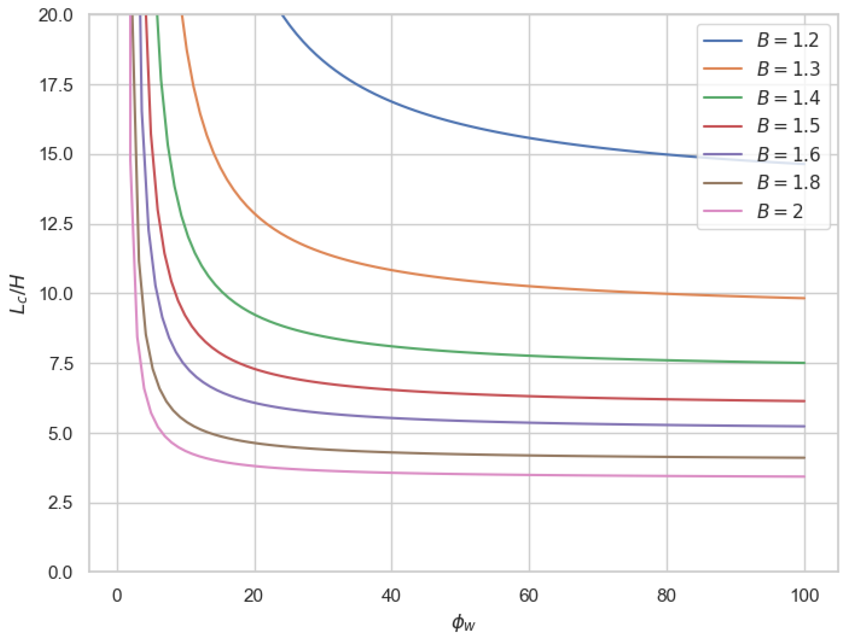
Figure 6.
Critical wind speed , critical wind factor , and high-wind asymptotic distance-to-collapse as a function of the SAV ratio and the relative packing ratio . Heading fire collapse occurs whenever the midflame wind speed U exceeds the fuel-dependent threshold . This is equivalent to > .The 53 Scott & Burgan fuel models are displayed as colored numbers; the Anderson fuel types are prefixed with ’A’. The x-axis is the Surface-Area to Volume (SAV) ratio (higher for finer fuels). The middle y-axis (log scale) shows the relative packing ratio , quantifying fuel bed compactness (higher means more resistance to convective heat transfer). is a characteristic length scale for heading fire collapse, defined as the distance at which the heading fire collapses to a pointed shape when ignited from a wind-perpendicular line segment of half-length H, in the limit of high wind speeds.
Figure 6.
Critical wind speed , critical wind factor , and high-wind asymptotic distance-to-collapse as a function of the SAV ratio and the relative packing ratio . Heading fire collapse occurs whenever the midflame wind speed U exceeds the fuel-dependent threshold . This is equivalent to > .The 53 Scott & Burgan fuel models are displayed as colored numbers; the Anderson fuel types are prefixed with ’A’. The x-axis is the Surface-Area to Volume (SAV) ratio (higher for finer fuels). The middle y-axis (log scale) shows the relative packing ratio , quantifying fuel bed compactness (higher means more resistance to convective heat transfer). is a characteristic length scale for heading fire collapse, defined as the distance at which the heading fire collapses to a pointed shape when ignited from a wind-perpendicular line segment of half-length H, in the limit of high wind speeds.
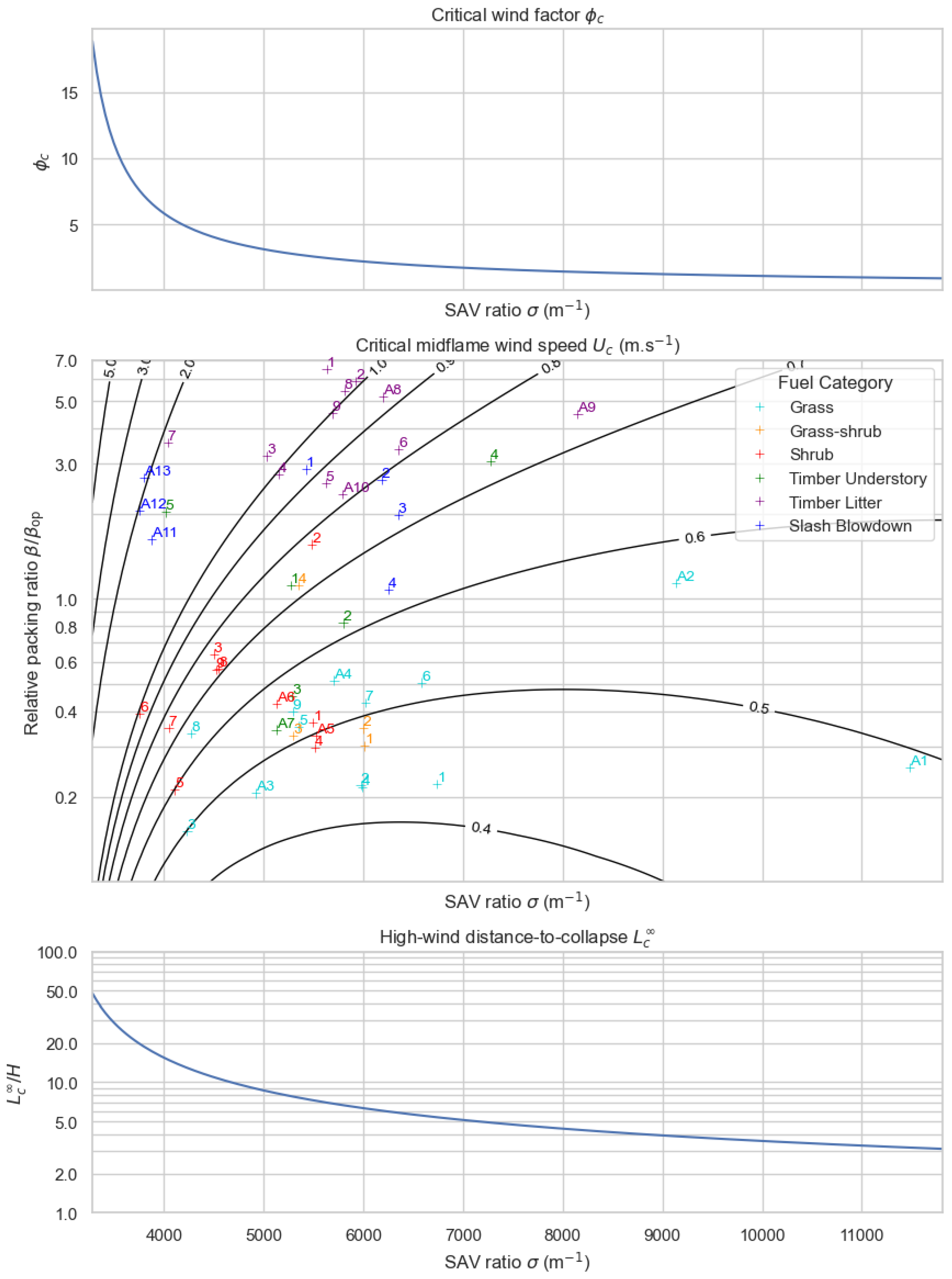

Table 1.
Main notation used in this paper.
| Symbol | Unit | Meaning |
|---|---|---|
| - | (front-normal) unit vector (2D vector) | |
| rad | Azimuth (typically, the angle from downwind to front-normal direction) | |
| m/s | Rothermel no-wind no-slope spread rate | |
| m/s | Rothermel heading fire spread rate: (equation 2) | |
| m/s | Front-normal spread rate (Equations 8 and 9) | |
| t | s | Time since ignition |
| U | m/s | Midflame wind speed |
| - | Rothermel wind factor (equation 3): | |
| B | - | Fuel property: wind exponent |
| m/s | Fuel property: characteristic wind speed | |
| - | Critical wind factor for heading fire collapse (Equation 14): | |
| m/s | Critical midflame wind speed for heading fire collapse (Equation 13) | |
| H | m | Half-length of the initially ignited line segment |
| m | Distance-to-collapse from cross-wind line segment (Equation 26) | |
| s | Time-to-collapse from cross-wind line segment (Equation 27) | |
| - | Supremum (≈ “maximum”) of a set A of real numbers | |
| - | Infimum (≈ “minimum”) of a set A of real numbers | |
| Magnitude of a vector | ||
| Dot product of vectors and | ||
| m | Position in the plane (2D vector) | |
| s/m | Inverse spread rate vector (2D vector) | |
| s | Time-of-Arrival function | |
| - | Indicator function of a set S (Equation A1) | |
| Convex conjugate of f (Equation A2) |
Table 2.
Fuel properties computed for a sample of fuel models.
| Fuel model number | class | SAV ratio | Relative packing ratio | ( | B | Wind factor, 6 mi/h | Wind factor, 12 mi/h |
|---|---|---|---|---|---|---|---|
| 2 | Grass | 9133.913 | 1.14 | 0.52 | 1.83 | 20.5 | 72.8 |
| 9 | Timber Litter | 8148.887 | 4.50 | 0.61 | 1.72 | 12.9 | 42.7 |
| 102 | Grass | 5971.257 | 0.22 | 0.25 | 1.46 | 31.1 | 85.3 |
| 165 | Timber Understory | 4014.454 | 2.03 | 0.34 | 1.17 | 11.1 | 25.1 |
| 188 | Timber Litter | 5807.777 | 5.42 | 0.57 | 1.43 | 9.2 | 25.0 |
Disclaimer/Publisher’s Note: The statements, opinions and data contained in all publications are solely those of the individual author(s) and contributor(s) and not of MDPI and/or the editor(s). MDPI and/or the editor(s) disclaim responsibility for any injury to people or property resulting from any ideas, methods, instructions or products referred to in the content. |
© 2026 by the authors. Licensee MDPI, Basel, Switzerland. This article is an open access article distributed under the terms and conditions of the Creative Commons Attribution (CC BY) license (http://creativecommons.org/licenses/by/4.0/).
Copyright: This open access article is published under a Creative Commons CC BY 4.0 license, which permit the free download, distribution, and reuse, provided that the author and preprint are cited in any reuse.