Submitted:
22 February 2026
Posted:
26 February 2026
You are already at the latest version
Abstract
Virtual Power Plants (VPPs) face significant challenges in managing the uncertainty and
variability of distributed energy resources (DERs), which can result in high trading risk
and deter investment. This paper proposes and evaluates two advanced optimisation
techniques—stochastic programming and robust optimisation—to derive risk-aware bidding
strategies for VPP participation in the day-ahead and balancing electricity markets. These
methods are benchmarked against a deterministic, expectation-based model. The novelty
of this work lies in the comparative application of stochastic and robust frameworks to VPP
bidding strategy design under real-world uncertainty, the introduction of scenario-based
wind and conventional generation models, and the integration of energy storage into the
optimisation framework to assess its impact on profitability and risk mitigation. Through
a series of simulations using actual market data from the UK (Elexon), we evaluate three
generation portfolio configurations—conventional, renewable, and aggregated. The results
show that while stochastic optimisation consistently achieves the highest expected profit, the
robust model ensures the highest minimum profit under worst-case conditions. Moreover,
combining DER types and integrating battery storage further enhances profitability and
reduces exposure to imbalance penalties. These findings provide valuable insights for the
development of intelligent, risk-aware trading strategies for VPP operators.
Keywords:
virtual power plant
; distributed generation
; electricity market
; optimisation
1. Introduction
Small, individual distributed energy resources (DERs) generally lack the financial capacity and risk management ability to engage directly in electricity markets. Their limited scale and exposure to significant production and market uncertainties make active participation difficult. This challenge is especially evident in markets where imbalances created by participants are penalised with charges that reflect the actual costs incurred. Due to forecast errors and dynamic changes in load and available energy resources, some imbalances inevitably occur during the real-time operation. By leveraging the concept of Virtual Power Plants (VPPs), distributed energy resources (DERs) can obtain access and visibility across various energy markets. Through the market intelligence provided by VPPs, these resources are able to strengthen their position and enhance opportunities for profit maximisation. At the same time, system operators benefit from the more efficient utilisation of available capacity and improved overall system performance. To ensure real-time balancing of supply and demand, operators typically maintain a certain level of reserves. These reserves are activated in case of imbalance between generation, production and demand [1]. To counteract these issues, small DER customers typically sell their electricity output, when it generates, at pre-agreed prices to an electricity supplier. Thus, it avoids exposure to imbalance cost. Since the supplier assumes the associated risks, the fixed contract prices are usually set below the true market value of the energy produced by DERs [2]. This work will investigate the optimisation approaches and the integration of individual DERs to manage the trading risk in energy markets and benefit from VPP market research intelligence to popularise their trading position and provide more opportunities to maximise the revenue. System operations can benefit from the optimal use of all available capacity and increased efficiency of the system. Coordination of distributed energy resources through VPP frameworks is increasingly facilitated by distributed optimisation techniques [3].
The purpose of grouping distributed energy resources (DERs) into a commercial Virtual Power Plant (VPP) is to allow them to participate in the market in a manner similar to conventional power stations. The chosen aggregation strategy should minimise imbalance risks compared to the operation of individual DERs, while at the same time enhancing the overall commercial prospects of the portfolio. This approach must also account for the uncertainties associated with the availability of each resource. To achieve this, the DER portfolio can be represented using stochastic programming, which determines the optimal quantities of electricity to commit in future markets so as to maximise the overall value of DER output [4].
This paper investigates the commercial framework and the aggregation on individual DERs to manage their risk and to maximise their capital returns. It provides the general strategy for offering energy on day-ahead and forward markets, by optimising the VPP portfolio and maximising the expected profit of VPPs. The paper is structured as follows: Section 2 describes the optimisation methodologies used throughout this paper. Section 3 introduces optimisation and risk management approaches including stochastic, expectation-based offer, robust and storage models. Section 3 also shows case studies and simulation results, followed by a discussion. Finally, Section 4 presents our conclusion.
2. Methodology
2.1. Stochastic Model
Stochastic programming is one of the techniques used to optimise decisions, taking uncertainty into consideration. These kinds of uncertainties usually evolve according to a multivariate stochastic process that can be estimated by a scenario tree.
The proposed model enables the participation of Combined Heat and Power–District Heating (CHP-DH) units and renewable energy sources (RESs) in the electricity market, while also allowing for the evaluation of different bidding strategies for Virtual Power Plants. By utilizing the operational flexibility of CHP-DH systems, the model can mitigate the uncertainties associated with day-ahead price fluctuations, imbalance costs, and renewable generation forecasts [14]. It is a mathematical computation tool that works to optimise marketing and production problems considering uncertainty [4]. The portfolio strategy is modelled to maximise or minimise the expectation of the function of decisions under the prevailing of uncertain variables. Several factors affecting the supply of electricity are evaluated using a mathematical formula that returns the most optimal combination of strategies [6].
The DER portfolio is faced with uncertainty in forecasting the required market output and the electricity prices. Our task is to come up with a strategy that will provide the maximum profit based on market evaluation and future predictions. Commercial aggregation of DERs with output uncertainty is now a reality in the power supply grid [6]. The system is facing uncertainty in its operations due to frequent power outages, the variability of the primary sources of energy and a functional pattern characterised by non-electricity output requirements. Stochastic programming helps to settle the imbalance using a system sell price for those who are willing to take a long-term engagement in the UK energy markets [7]. A commercial Virtual Power Plant (CVPP) consolidates the operational characteristics and cost structure of a distributed energy resource (DER) portfolio into an aggregated profile. Within the wholesale energy market, a CVPP facilitates trading, portfolio balancing, and service provision by submitting bids and offers to the system operator [8]. The CVPP operator—often an energy supplier or a third-party aggregator with market access—collects and integrates information such as marginal costs, metering records, load forecasts, operational parameters, market data, and locational inputs. This aggregation supports the formulation of forward contracts, system balancing activities, and the scheduling of distributed generation (DG), demand, and technical virtual power plant (TVPP) parameters [9].
One of the most widely used stochastic programming models is a two-stage linear program (Figure 1). In this model, the decision sets can be divided into two stages: In the first stage, the decision should be made based on a deterministic approach. These decisions are normally called “here and now decisions.” However, decisions at the second stage must be made after the random event occurs, and the decision from the first stage should be considered [10]. The approach applies a linear programming model that incorporates forecasted prices for both the spot and balancing markets, which are accessible to the portfolio operator. These forecasts provide the anticipated price trajectories for each half-hourly interval, including the minimum expected values at every time step [6].
A basic linear programming formulation, widely used for two-stage stochastic programming problems, is given below (1)–(4):
In this formulation, x denotes the first-stage decision variable, with the associated vectors and matrices s, b, and A. In the second stage, multiple random outcomes may occur. For each realisation of w, the parameters , , and are revealed, where q, h, and T represent random variables capturing the underlying uncertainty. The parameter is dependent on w and represents the mathematical expectation. The parameter is a second-stage decision which should be considered to determine the resource decisions. The is a second-stage objective expectation and is a deterministic term [10].
The second-stage function for a given w is formulated as (5):
The formulation of a deterministic linear programming approach is given below (6)–(8):
Generally speaking, stochastic optimisation provides better solutions in comparison to the expectation-based approach by considering random events. In most cases, the expected profit from the stochastic approach is higher than the deterministic one when all uncertainties are considered [6].
The proposed approach applied to the case studies to calculate the expected profit function is formulated as shown in (9):
where , , and are the market price (MP), system sell price (SSP), and system buy price (SBP), respectively. and are energy surplus and energy shortage, and and are the generation cost and output of the individual generator. The i, t, and s indicate the generator, time, and scenarios, respectively.
Equation (10) sets the upper bound of generation output:
The upper bounds of available capacity are also applied to intermittent renewable generators (e.g., wind), representing the available wind power output in scenario s. The relationships among energy surplus, shortage, generator outputs, and the offered quantities are defined by the energy balance constraint (11):
2.2. Expectation-Based Offer
Similar to the stochastic approach, the expectation-based offer can also be applied for calculation, with the difference that the expectation-based offer formulation does not contain scenario terms and the equation for surplus and energy. At the first stage, we calculated the expectation-based offer based on the pure deterministic model without considering imbalance prices or risks of full generator unavailability. Then in the second stage the stochastic model is applied, subject to uncertainty and generator unavailability to assess the performance of the offer against risk. The model uses the maximum value for the offer, which is the maximum available generation.
2.3. Robust Model
Robust optimisation (RO) has been widely employed to address profit-maximisation problems in areas such as electricity markets and portfolio management. By carefully tuning the control parameters, this method ensures feasibility across all possible realisations of uncertain variables within specified confidence bounds, while also guaranteeing optimality under their worst-case outcomes [14]. Furthermore, RO has been applied to various power system challenges, including the development of offering strategies under uncertainty [11]. In the proposed RO framework, different control parameters are introduced to represent the degree of conservatism in the solution, such that the optimisation focuses on the worst-case scenario corresponding to a chosen robustness level.
Using the standard robust model, we obtain the following model for the robust optimisation for the electricity market bidding strategy using wind generation as an example:
where is the day-ahead market price, is the offered quantity, and are imbalance prices for SSP and SBP, and are parameters to control the robustness of the model, and and are dual variables related to uncertainty in market prices and generation.
The objective function (12) is designed to maximise profit under the worst-case bidding scenario. To account for uncertainty in both prices and generation, the non-negative robustness parameters , , , and are introduced. These parameters capture deviations from the mean values of the corresponding uncertain variables. Specifically, , , and can take values within the interval , where 0 corresponds to a non-robust solution and to the most conservative one. In contrast, ranges between 0 and 1, thereby controlling the robustness level against renewable generation uncertainty.
The first three constraints (13)–(15) address the uncertainty in market prices that directly influence the objective function. The subsequent constraints (16)–(18) ensure that both wind and conventional generation remain within their available capacity limits, under the condition that no more than uncertain coefficients deviate from their mean values within the forecasted confidence interval.
2.4. Generic Storage Model
Energy storage can provide various benefits to the energy industry and services to support grid operation. Thus, the integration of energy storage technologies will increase the efficiency of the system and provide a level of adaptability against the uncertainty and variability characteristic to energy systems with a high integration of intermittent renewable generation and supplying demand at peak times to decrease generation costs [13]. Energy storage refers to types of technologies which can store electricity for later use. In addition to providing cost-effective usage of electricity, storage is also used to improve power reliability. Usually, the energy storage facilities are defined by three parameters: efficiency, rated capacity and charging/discharging power [14]. Below, the storage parameters used in this work are shown:
The main challenge of adding storage to the model is to decide how to choose an optimal bid for the day-ahead market, considering market price uncertainty, and how to plan the charging and discharging schedule for the storage. In our model, we are considering a generic energy storage facility which makes it possible to store energy at non-peak times and discharge at peak times—energy arbitrage as shown in Table 1. The operation of energy storage is modelled by the following constraints (19)–(21):
The objective function to be maximised is the expected profit that results from buying energy to charge the storage plant during low price periods and to later sell in periods with high market prices. A binary variable is used to model the charging () and discharging () state of the storage. The following constraints (22) and (23) are used to balance the stored energy in each period due to the charge and discharge actions and to bound the stored energy in each period to the capacity limit:
The roundtrip efficiency factor represents the energy losses during the conversion of energy in the storage plant during charging periods. To integrate the storage operation model into the existing model, we must consider that the offered quantity must now represent the injected power from the storage plant (24).
All models were simulated in the Fico Xpress-Mosel software, version 9.0.
3. Case Studies
3.1. Description
The developed methodologies have been applied to a range of case studies. In each case study, the optimisation of the aggregated DER portfolio is investigated, and the effect of different constraints on it, such as energy storage, is evaluated. The impact of having only conventional or intermittent generation and a combination of those two is investigated in the studies.
asIn Case A, only conventional generation, in which there is uncertainty regarding the accessibility of producing power, is considered. This uncertainty in generator output is characterised as two stages: either fully available or not fully available. For each generator, the specific availability probabilities are assigned. Case B, on the other hand, considers only renewable generation (wind generation) by having five wind generation levels with an assigned output, initial and final probabilities. Using linear interpolation, the specific probabilities for the scheduling period are calculated, considering that the wind forecast is more reliable for a shorter time and vice versa.
The last case is Case C, which is an aggregation of conventional and wind generations. The same parameters and assumptions are also applied in this case to compare the value of aggregated DERs with other cases.
3.2. Market Data
The half-hourly market, system sell and system buy prices considered in this study were obtained from the Elexon website for May 2008, considering only workdays [15]. As shown in Figure 2, the three median price forecasts were constructed based on Elexon data: market price (MP), system sell price (SSP) and system buy price (SBP). Additionally, for each of these prices, the high- and low-price series were derived, and it was assumed that the probability of median prices was 0.6 and the probability of high/low prices was 0.2 for each. The second plot in this figure presents a higher resolution of the first 14 time periods of the considered day.
Alongside with other assumptions introduced in the previous chapter, it is always assumed that the SBP is higher than the MP, while the SSP is lower than the MP throughout the day for price scenarios. Although the cost structure remains constant throughout the day, the variation between price scenarios depends on system actions. In the initial 6–7 h, market prices are relatively stable, ranging between 40 and 60 GBP/MWh. However, from point 15 onwards, prices exhibit significant fluctuations, with peaks such as 150 GBP/MWh at point 35. It is therefore essential to examine the relationship between day-ahead and imbalance prices. For example, at period 35 the gap between the market price (MP) and the system buy price (SBP) is considerably high. Under such conditions, submitting large energy bids becomes risky, as any shortage would result in steep imbalance costs due to the high SBP compared with the MP. Conversely, after point 43 the difference between the MP and SBP becomes small, which reduces the imbalance risk and enables the system to offer larger quantities of energy.
3.3. Generation Data
The system includes four conventional generators, each characterised by distinct capacity, generation cost, and availability, with a combined nominal output of 30 MW. When availability is taken into account, the expected total capacity reduces to 19 MW. Since each generator can exist in one of two states—either fully operational or unavailable—there are possible generation states used to represent all potential outcomes in each period. Each state is assigned a probability value based on the available data, as summarised in Table 2.
On the other hand, wind generators are defined by wind generation levels with power output and assigned probabilities. Specific probabilities for each period and wind generation levels were constructed using the linear interpretation of initial and final probabilities and the expected capacity of generation levels as shown in Table 3.
3.4. Results and Discussion
3.4.1. Models Without Storage
The following graphs show the optimal offer and expected profit from stochastic and robust optimisation techniques for all generation cases (conventional, renewable, and aggregated). All graphs are compared to each other and the purely expectation-based offer and profit. As shown in Figure 3, in the first periods, the stochastic offer is significantly high, since the difference between the SBP and MP is low. Consequently, the impact of shortage costs is low as well. From point 4, due to a decrease in the SBP, the stochastic offer starts to increase until point 6, from where all prices are stable with small fluctuations. It starts increasing from point 11, peaking at 15 when market price also increases while the SSP stays stable. When the SBP has its highest value (point 35), the stochastic offer decreases rapidly to avoid the risk of paying high SBP. The expectation-based and robust offers show a similar pattern as the optimisation models of these two are similar. However, as the robust model considers additional parameters to adjust the robustness of the system based on the worst-case scenario, in the periods where SBPs are high, the robust offer performs better as it considers the risks of the units not being available to generate in addition to high imbalance prices.
The stochastic and robust offers have different patterns, but the profit graphs look similar (Figure 4) since the robust bid presents a more conservative offer. Even though the offer is always lower, hence the market revenue being lower, this leads to a lower payment of shortage costs and generation costs, and also a higher surplus revenue. Table 4 presents a breakdown of the components of the expected profit for all offers. Stochastic profit outperforms mainly in two time periods, points 23 and 35. Despite the stochastic offer being quite low at these points, the high MP and SSP increase the profit. By the end of the day, the stochastic profit starts decreasing due to a decrease in market price, while the offer reaches the second peak at the same points (44–47) because the SBP at this point is almost the same as the MP, which means there is no risk of being penalised by energy shortage. In addition, at these points, the expectation-based and robust offers remain the same with a decrease in profit.
As mentioned in the previous case, the expectation-based offer and robust offer are fairly similar in shape but different in quantity, as they remain either constant (robust offer) or decrease slightly (expectation-based offer). For Case B, the offer (Figure 5) is a fixed amount of energy throughout the day, with the robust model offering almost half of the expectation-based offer. The robust model is highly dependent on the robustness parameters, which will be discussed later. From the offered pattern, it can be easily seen that the stochastic offer is very sensitive to changes in SBP. Throughout the day, the stochastic offer shows different trends, increasing when the SBP decreases and vice versa. During the period from points 12 to 18, the offer is fluctuating because of an increase in the SBP and the difference between the SBP and MP, while from point 19 it stays constant due to cost differences between the MP, SBP, and SSP. The same occurs with conventional generation; the lowest offer value is also at point 35, when we have the highest SBP, to avoid the payment of system shortage costs. Since the difference between the MP and SBP starts to increase from point 31 to 35, the stochastic offer significantly decreases due to the very high SBP. The offered quantity peaks again at periods 43–44 due to a sharp decrease in SBP (Figure 5).
An interesting observation is that throughout the day, the stochastic and robust offers show different trends. For instance, the stochastic offer fluctuates several times in a day while the robust offer is consistent all day long, but if we look at the profit curve, we can see fairly similar line shapes. The same principle for conventional generation is applied here. As the offer is significantly lower than the other two (on average 10 MW lower), the expected shortage costs are much lower while the surplus revenue is higher, thus reducing the difference between the curves (Figure 6).
As a result, the stochastic offer shows better performance in terms of adapting uncertainties, giving higher profit throughout a day. During the peak hours when the SBP is significantly high, the stochastic model offers a small amount of energy, avoiding the risk of paying the SBP. The robust offer can be considered as the worst-case offer/profit but with minimum risk. It takes into account all risks and uncertainties and offers an amount of energy with minimum risk (Figure 7 and Figure 8).
From the comparison shown in Figure 9, we can observe that in all cases the stochastic model gives higher profit in comparison with the robust and expectation-based offers, which is due to the better adaptability of a stochastic offer to uncertainties in market and imbalance prices. The stochastic offer is determined by modelling all scenarios and realisations and finding the offer and the recourse actions (payment of shortage costs or selling surplus energy) that lead to the highest profit. Through this optimisation, it is possible to know when to bid more than expected, i.e., when the probability of paying high shortage costs is lower, and when to bid lower, i.e., when the probability of paying high shortage costs is higher. This behaviour can be seen in Figure 7 for the periods 11–12, 13–20, and 43–48 where the stochastic offer is higher than the expectation-based approach, while in periods 32–37, it is lower. By knowing when to offer more or less, the stochastic offer presents a better performance against the risk of paying shortage costs.
3.4.2. Wind Forecast Uncertainties
The accuracy of wind forecasting significantly influences VPP performance and bid risk exposure [16]. To see the effect of wind forecast uncertainties on offered quantities, wind generation forecasts with different probabilities but the with same output were assessed. The Table 5 shows wind generation data that was used for the comparison:
As a result, only two comparison graphs (Figure 10 and Figure 11), stochastic and expectation-based, are shown below, since the changing in wind forecast does not affect the robust model offer which shows the same amount: a 13.75 MW offer in both cases. The expectation-based offer shows a slight decrease in the offered quantity and increases indifference compared to the first case’s offer. This behaviour reflects the difference in wind forecasts, as expected wind generation levels change due to the varying nature of probabilities.
Regarding the stochastic offer, there is a variation for some periods. For instance, during periods 5–7 and 16–19, the offer for Case B1 is higher than Case B2, which can be explained by uncertainties in different wind forecasts as well as the difference between market, system sell, and system buy prices for adjustments. Given the reduced expected wind generation levels for forecast B2, it is expected that the offer will be lower as it is more exposed to paying high shortage costs than forecast B1.
3.4.3. Best Case vs. Worst Case
The comparison shown in Table 6 presents the highest and lowest profits achieved by each type of offer and for each case study to determine the best and worst scenarios, respectively. These values were obtained by calculating the daily profit for each combination of price forecasts and generation state/level. It can be observed that the best profit is always achieved in a high-price scenario and when all conventional generators (CG state 16) and wind (WG level 5) generators are available for all periods. The worst profit occurs when none of the conventional generators are available and the wind generation is at level 1, the minimum, for all periods. As seen in the following table, for Cases A and C, all the worst profits are negative, while for renewable generation cases the profits are positive. The robust model gives the highest worst-case profit in comparison with other models, which is significantly high in Case B (GBP 5409), while the stochastic and expectation-based offers show worst-case profits of only GBP 66 and GBP 95, respectively. The high value in Case B can be explained due to the fact that the submitted offer (13.75 MW throughout the day) is much closer to the minimum wind generation level (5 MW) than the other two offers (which is translated into a difference of 8.75 MW for the robust offer, approximately 20 MW for the expectation-based offer, and a minimum of 15 MW and maximum 35 MW for the stochastic offer) and leads to the payment of lower shortage costs for the robust offer than the other two. The worst-case profits are negative for the robust optimisation models, as the robust parameter for the generator was considered to be 0.5. By considering a fully conservative optimisation, i.e., maximum robustness (all robust generation parameters are 1.0 and all robust price parameters are 48), it is expected that all energy sold in the market would be considered an excess from the offered quantity (either 0 MW for conventional generators or the minimum generation level for wind generation) and the expected profit would be mostly composed of surplus revenue and generation costs. In these conditions, it would be expected that the VPP would not have to pay shortage costs. In terms of the worst-case scenario, the robust model performs better than the other two models. The highest best-case profit comes from the stochastic model in all cases.
3.4.4. Models with Storage Constraints
The following graphs show the comparison of the offers given by stochastic and robust methods with and without storage. The results indicate that storage can improve the profitability of the VPP, due to the ability to store energy when prices are low and sell when they go up—energy arbitrage—and in the case of the stochastic model to manage energy shortages.
In Figure 12, Figure 13 and Figure 14, the charging and discharging time periods can be clearly seen. For example, in the robust model, full charging and discharging occurs once a day at the time periods between points 6 and 11 and between points 22 and 27, respectively, while in the stochastic model, both charging and discharging occur at different times during the day which can be seen from a comparison of graphs with and without storage. Following the stochastic nature, charging occurs when the prices are low (or the difference between the MP and SBP is low) and discharging when prices are high. It is worth noting that when the model with storage offers less energy than the model without storage, the storage plant is in the charging state and vice versa.
As storage technologies are used to improve the integration of distributed energy resources, the comparison of profits from different optimisation techniques was calculated. Table 6 shows the expected profit from the expectation-based, stochastic, and robust offers for each case study. As can be observed in Figure 15, the stochastic offer gives the highest profit in all cases, while the robust offer has the lowest profit.
3.4.5. Comparison of Different Storage Capacities
To incorporate electricity storage in this work, a simple generic storage model with a maximum charging/discharging rate and stored energy capacity was considered. The relation between different storage capacities, charging/discharging rates, and the VPP’s expected profit are studied in this section and compared. As shown in Table 6 and Figure 12, the expected profits for all cases increasingly align with the increase in storage capacity in almost the same manner, with the curves showing the same shape.
Using storage for aggregated systems is very beneficial in terms of profit. This can be seen from Figure 16, which shows the benefit of using aggregated generation and the effect of different storage capacities. It is very important to determine suitable storage capacity for the system.
As Table 7 demonstrates, it is more beneficial to have storage capacity at 5 MW for all optimisation models where it has the highest value, while it decreases significantly as capacity increases due to the need to procure energy to charge the battery.
3.4.6. Robust Level
The robust model has two types of coefficients to adjust the robustness of the system against uncertainties; one type is for prices (MP, SSP, SBP), and the second one is for generation (CG, WG). The parameters for prices and generation can take values between [0, 48] for the prices and [0, 1] per period for the generators. When both values are equal to 0, the model behaves in a non-robust way and does not consider risks associated with prices and other uncertainties for all periods. The model has the most robust results when both parameters take maximum values, 48 for the prices and 1 per each period for the generators. Figure 17 presents the comparison of profits for different robustness levels.
4. Conclusions
Stochastic optimisation techniques tend to adapt better to uncertainties, such as wind forecasts and imbalance prices. Therefore, it gives the highest profit for all evaluated models. However, this optimisation method highly depends on the quality of the scenarios considered to model generation and price uncertainties. On the other hand, robust optimisation can be considered for the worst-case optimisation of the VPP portfolio; in other words, it maximises the worst-case profits of the system, offering energy by taking the minimum risk associated with uncertainties. An important outcome from the results is the benefit of using aggregated generation. In all cases, profit from combined renewable and conventional generators is higher than the arithmetic sum of profits from an individual group of renewable and conventional generators. On the other hand, investing in energy storage can be beneficial for the system, as shown in the expected profit results (Table 6 and Table 7). The stored energy capacity and charging/discharging rate have a significant effect on the results and should be taken into account when deploying an energy storage system. The findings of the work can be summarised as follows:
- Robust optimisation will minimise the risk, especially if the worst condition occurs; this is facilitated by providing a sufficient amount of reserves to deal with uncertainty. However, this strategy also leads to less revenue from the day-ahead market and forward market due to the minimisation of risks.
- Due to its conservative nature, the robust model shows better adaptability to the risk profiles. This can be seen from Table 2, where the robust optimisation has the highest shortage and surplus revenue, even though the market price is lower in comparison to other approaches.
- Combining the portfolio of conventional and intermittent generation in the VPP portfolio increases the expected profit of the system. The robust approach especially gives significantly high revenue from the market (Table 8).
- The maximum profits from the market can be achieved from stochastic optimisation, which is most beneficial for all the case studies. However, it is less adaptable to risk profiles than a robust one.
- Investigating energy storage technologies is beneficial in terms of profit maximisation and choosing the best strategy to optimise the VPP portfolio. For the same capacity, the stochastic model has the highest profit for all case studies (Figure 7), but is the lowest in terms of aggregation benefit (Figure 8). However, it is important to choose the proper storage capacity to maximise the expected profit.
Author Contributions
Conceptualization, O.K. and D.P.; Methodology, O.K. and D.P.; Software, O.K.; Validation, O.K.; Formal analysis, O.K.; Investigation, O.K.; Writing—original draft, O.K.; Writing—review & editing, D.P.; Visualization, O.K. All authors have read and agreed to the published version of the manuscript.
Funding
This research received no external funding.
Data Availability Statement
The original contributions presented in this study are included in the article. Further inquiries can be directed to the corresponding author(s).
Conflicts of Interest
The authors declare no conflicts of interest.
Abbreviations
The following abbreviations are used in this manuscript:
| VPP | Virtual Power Plant |
| DERs | Distributed Energy Resources |
| CHP | Combined Heat and Power |
| TSO | Transmission System Operator |
| DG | Distributed Generation |
| DSO | Distribution System Operator |
| MAS | Multi-Agent System |
| DCVPP | Decentralised Virtual Power Plant |
| FDCVPP | Fully Decentralised Virtual Power Plant |
| CVPP | Commercial Virtual Power Plant |
| TVPP | Technical Virtual Power Plant |
| EMS | Energy Management System |
| LP | Linear Programming |
| CSP | Curtailment Service Provider |
| LSEs | Load Service Entities |
| UDC | Utility Distribution Company |
| ESP | Energy Service Provider |
| PBUC | Price-Based Unit Commitment |
| DA | Day-Ahead |
| CHP-DH | Combined Heat and Power–District Heating |
| WP | Wind Production |
| WPS | Wind Power System |
| LSVPP | Large-Scale Virtual Power Plant |
| DEMS | Distributed Energy Management System |
| PHEV | Plug-in Hybrid Electric Vehicle |
| RO | Robust Optimisation |
| SO | Stochastic Optimisation |
| MP | Market Price |
| SSP | System Sell Price |
| SBP | System Buy Price |
References
- Ruiz, N.; Cobelo, I.; Oyarzabal, J. A Direct Load Control Model for Virtual Power Plant Management. IEEE Trans. Power Syst 2009, 24, 959–966. [Google Scholar] [CrossRef]
- Pudjianto, D.; Ramsay, C.; Strbac, G. Virtual power plant and system integration of distributed energy resources. IET Renew. Power Gener. 2007, 1, 10–16. [Google Scholar] [CrossRef]
- Li, J.; Mo, H.; Sun, Q.; Wei, W.; Yin, K. Distributed Optimal Scheduling for Virtual Power Plant with High Penetration of Renewable Energy. Int. J. Electr. Power Energy Syst. 2024, 160, 110103. [Google Scholar] [CrossRef]
- Rahimi, F.; Ipakchi, A. Overview of Demand Response under the Smart Grid and Market paradigms. In Proceedings of the 2010 Innovative Smart Grid Technologies (ISGT), Gaithersburg, MD, USA, 19–21 January 2010. [Google Scholar]
- Liu, J.; Wu, J.; Lei, Z. Two-Stage Optimization Strategy for Market-Oriented Lease of Shared Energy Storage in Wind Farm Clusters. Energies 2025, 18(11), 2697. [Google Scholar] [CrossRef]
- Aunedi, M.; Strbac, G.; Pudjianto, D. Characterisation of portfolios of distributed energy resources under uncertainty. In Proceedings of the 20th International Conference and Exhibition on Electricity Distribution (CIRED 2009), Prague, Czech Republic, 8–11 June 2009. [Google Scholar]
- Rashidizadeh-Kermani, H.; Vahedipour-Dahraie, M.; Shafie-khah, M.; Siano, P. A Stochastic Short-Term Scheduling of Virtual Power Plants with Electric Vehicles under Competitive Markets. Electr. Power Syst. Res. 2021, 194, 107085. [Google Scholar] [CrossRef]
- Tarazona, C.; Muscholl, M.; Lopez, R.; Passelergue, J.C. Integration of distributed energy resources in the operation of energy management systems. In Proceedings of the 2009 IEEE PES/IAS Conference on Sustainable Alternative Energy (SAE), Valencia, Spain, 28–30 September 2009; pp. 1–5. [Google Scholar]
- Garcia-Gonzalez, J.; de la Muela, R.; Santos, L.; Gonzalez, A. Stochastic Joint Optimisation of Wind Generation and Pumped-Storage Units in an Electricity Market. IEEE Trans. Power Syst. 2008, 23, 460–468. [Google Scholar] [CrossRef]
- Wilson, J.; Birge, J.; Louveaux, F. Stochastic Programming. J. Oper. Res. Soc. 1998, 49, 897. [Google Scholar] [PubMed]
- Rahimiyan, M.; Baringo, L. Strategic Bidding for a Virtual Power Plant in the Day-Ahead and Real-Time Markets: A Price-Taker Robust Optimization Approach. IEEE Trans. Power Syst. 2016, 31, 2676–2687. [Google Scholar] [CrossRef]
- Bertsimas, D.; Sim, M. The Price of Robustness. Oper. Res. 2004, 52, 35–53. [Google Scholar] [CrossRef]
- Lever, A.; Sanders, D.; Lehmann, N.; Ravishankar, M.; Ashcroft, M.; Strbac, G.; Aunedi, M.; Teng, F.; Pudjianto, D. Can storage help reduce the cost of a future UK electricity system? Technical Report; Carbon Trust & Imperial College London, 2016. [Google Scholar] [CrossRef]
- Liu, Y.; Zhang, X.; Ma, Z.; Ren, W.; Xiao, Y.; Xu, X.; Liu, Y.; Liu, J. Risk-Aware Scheduling for Maximizing Renewable Energy Utilization in a Cascade Hydro–PV Complementary System. Energies 2025, 18(12), 3109. [Google Scholar] [CrossRef]
- Elexon.co.uk. Market Domain Data—ELEXON. 2016. Available online: https://www.elexon.co.uk/reference/technical-operations/market-domain-data/ (accessed on 31 August 2016).
- Jin, Y.; Gao, C. Market Applications and Uncertainty Handling for Virtual Power Plants. Energies 2025, 18(14), 3743. [Google Scholar] [CrossRef]
Figure 1.
Representation of the two-stage linear stochastic program [9].
Figure 1.
Representation of the two-stage linear stochastic program [9].
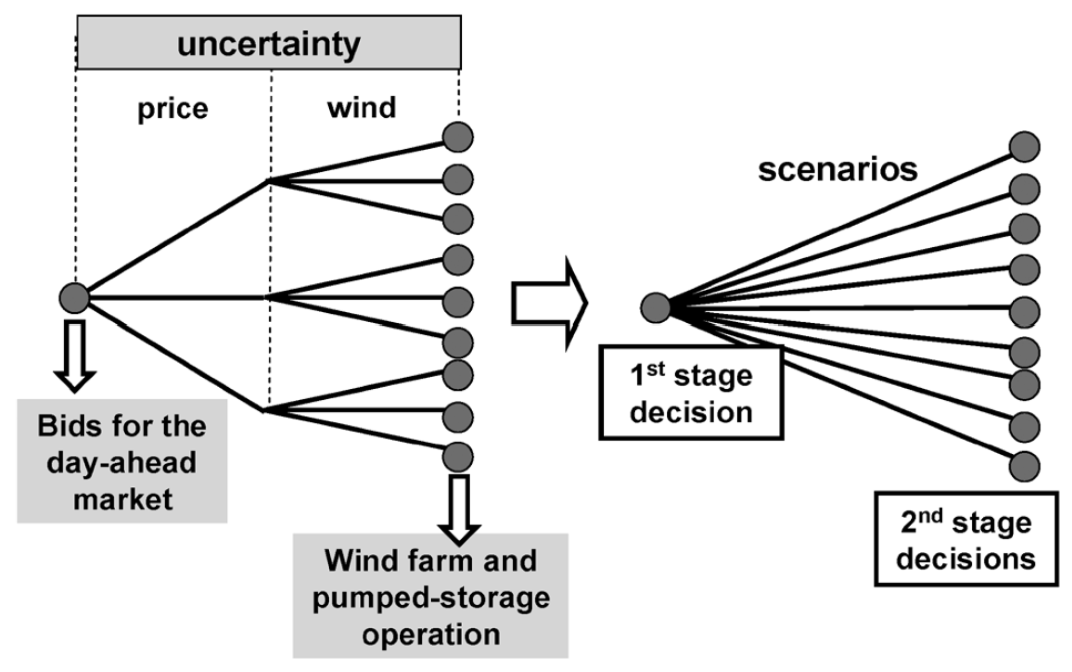
Figure 2.
Day-ahead market and imbalance price forecasts.
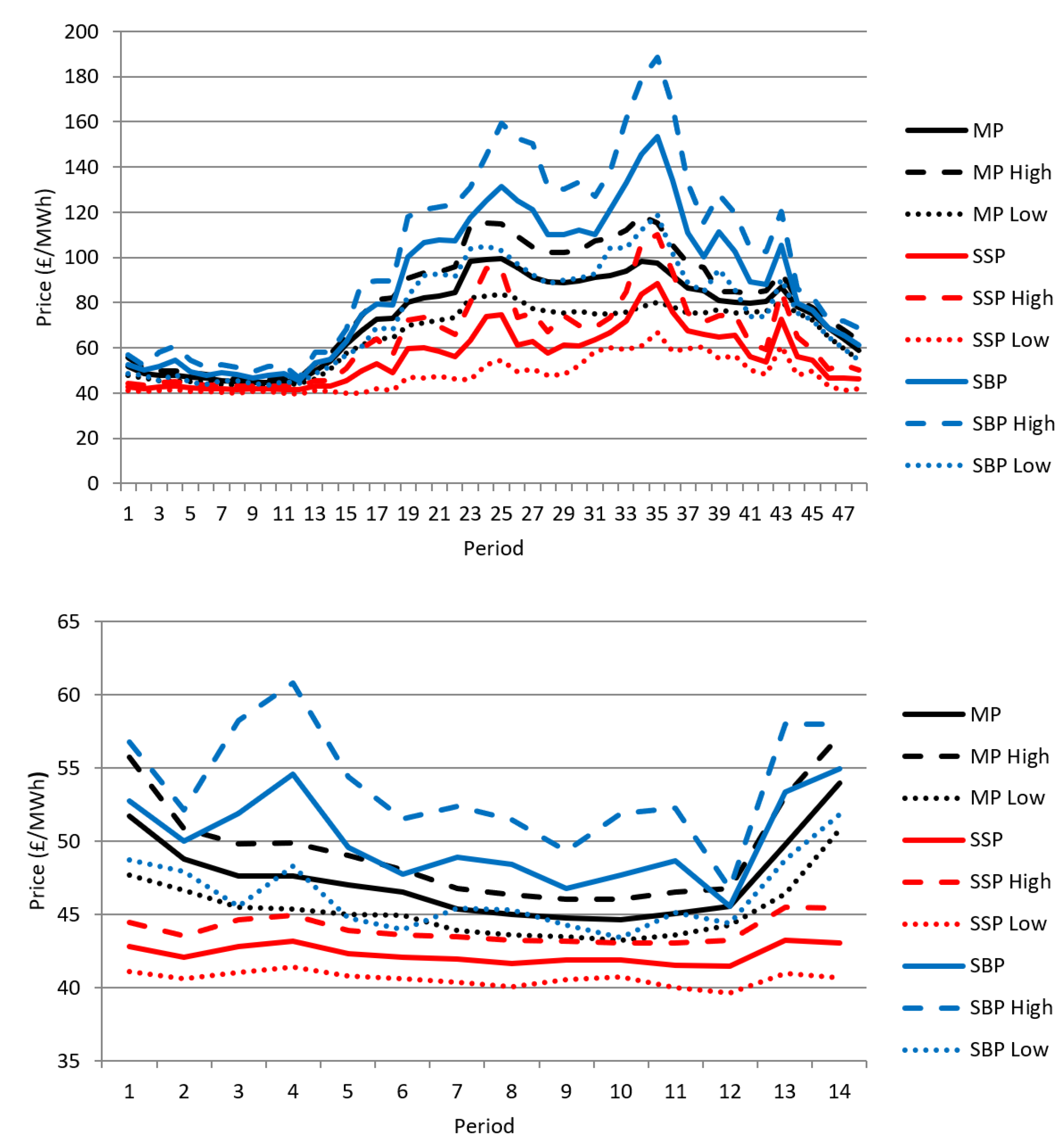
Figure 3.
Offered quantity for Case A.
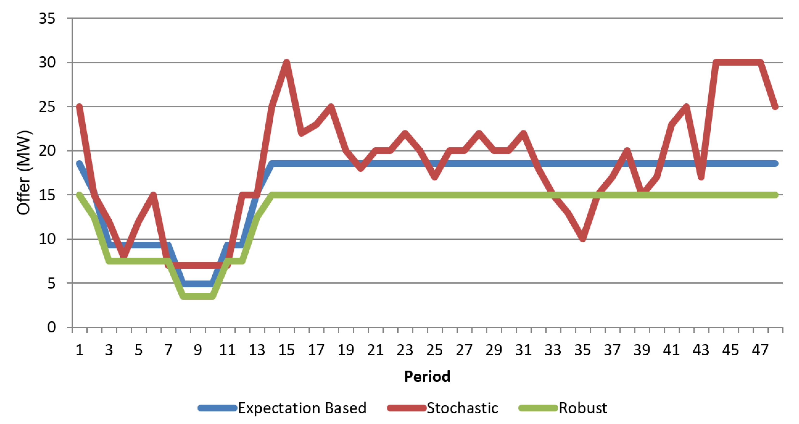
Figure 4.
Expected profit for Case A.
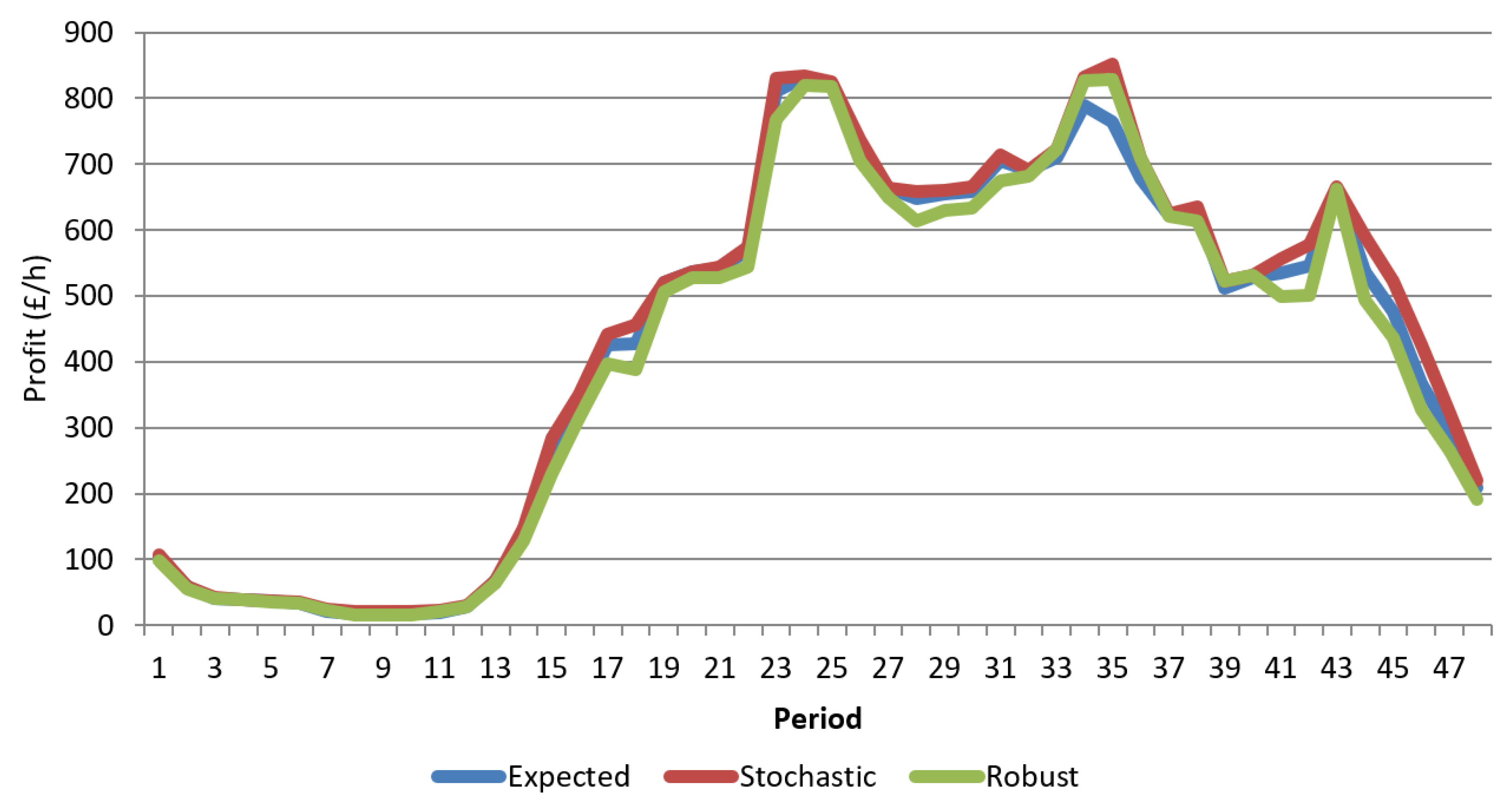
Figure 5.
Offered quantity for Case B.
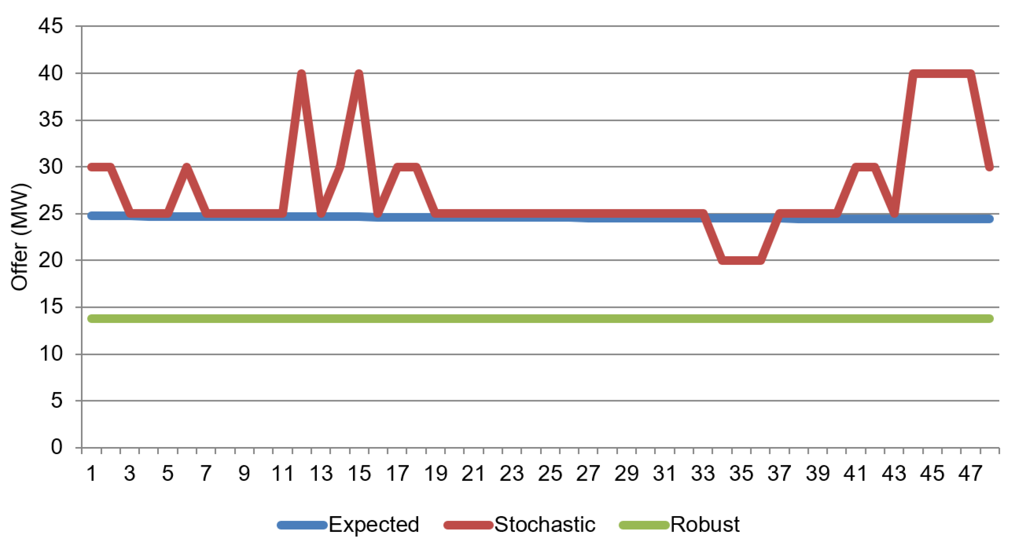
Figure 6.
Expected profit for Case B.
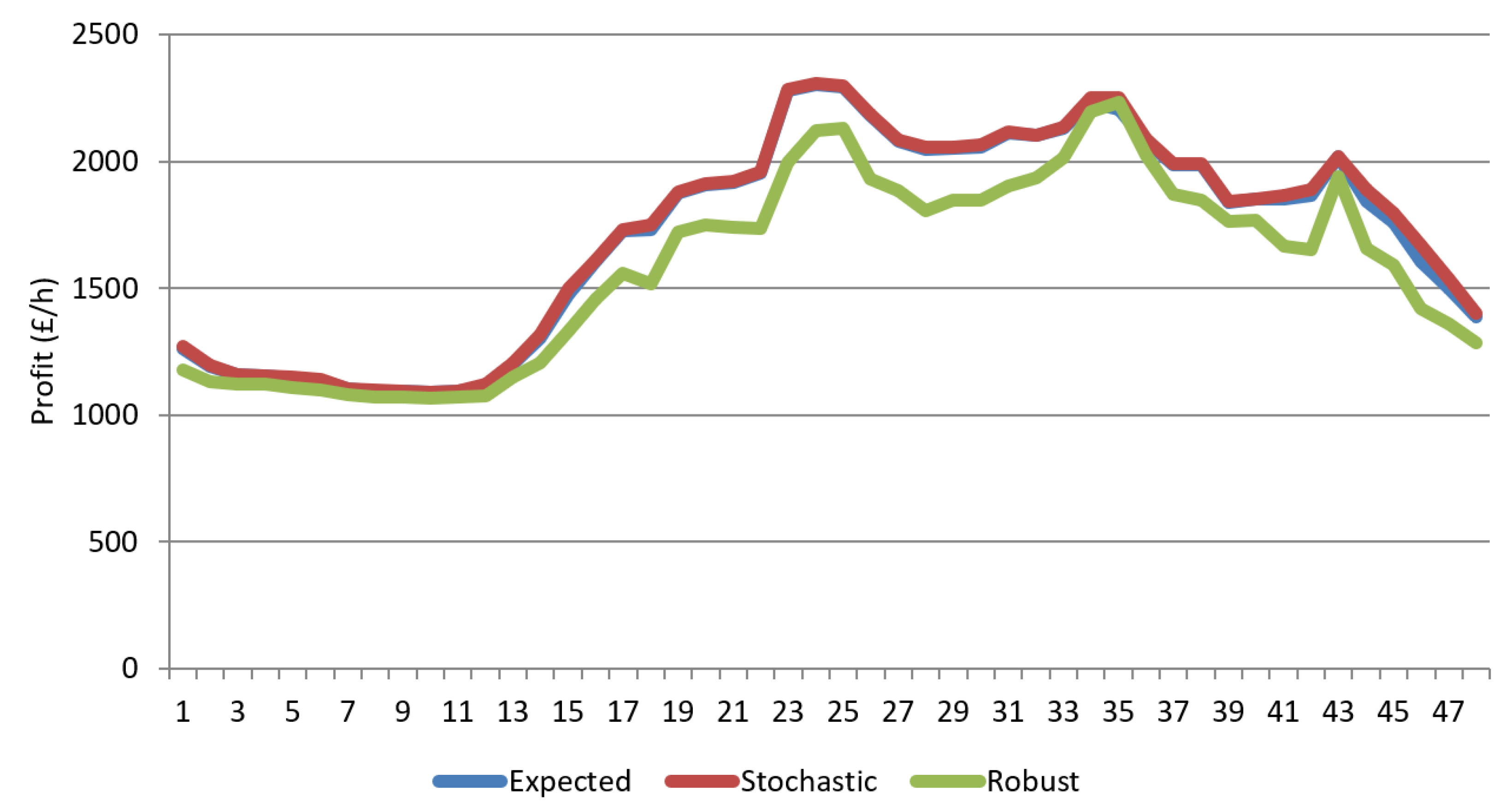
Figure 7.
Offered quantity for Case C.
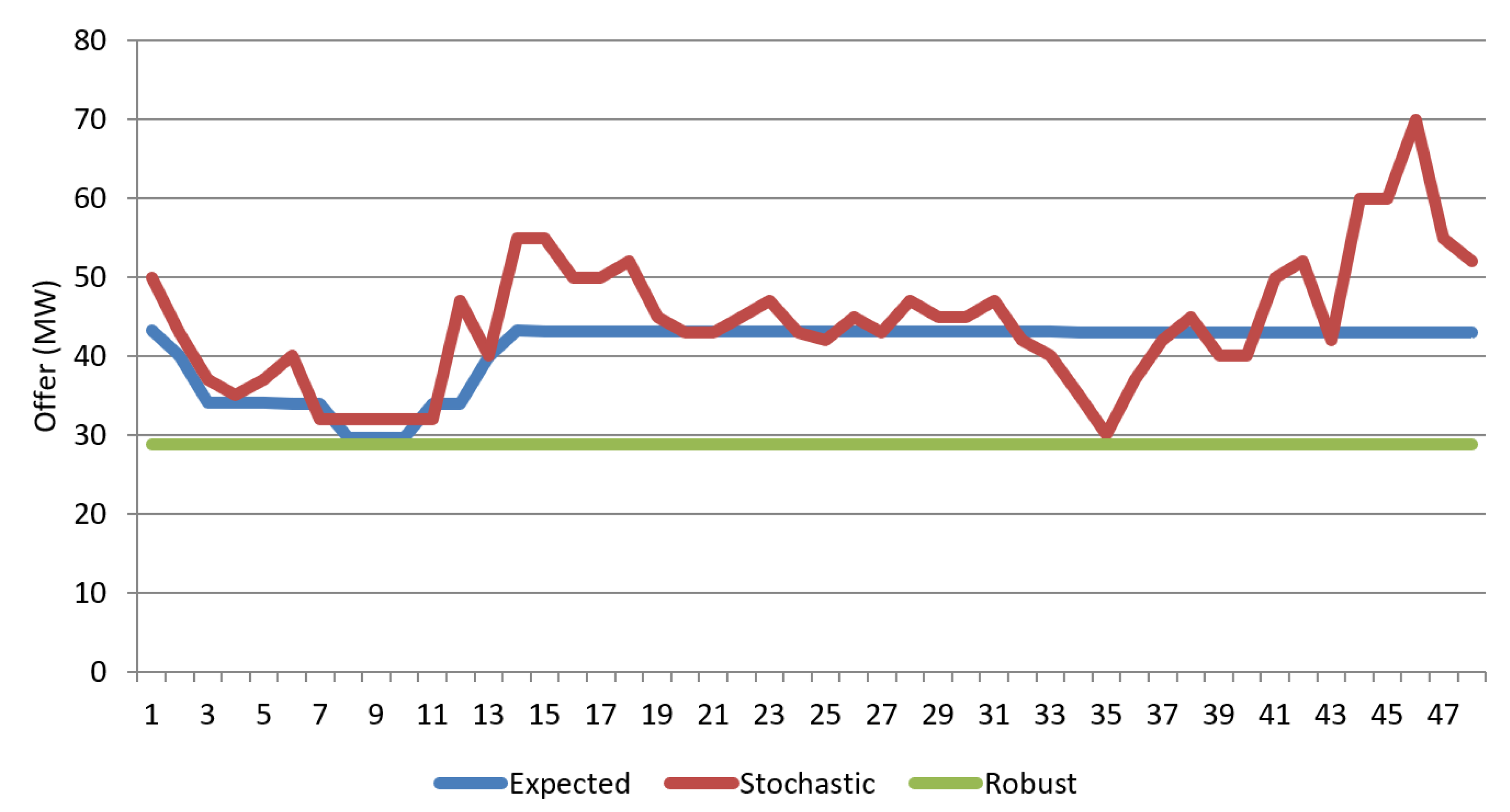
Figure 8.
Expected profit for Case C.
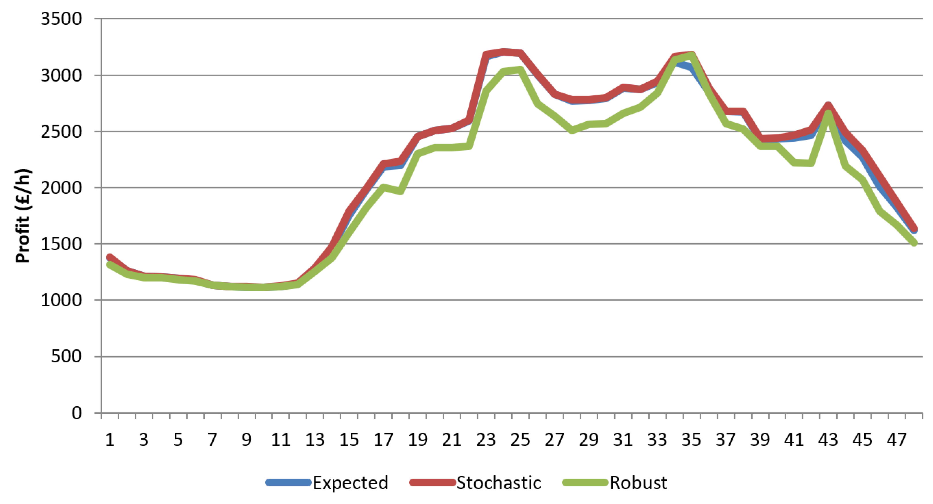
Figure 9.
Comparison of the expected profits for different cases.
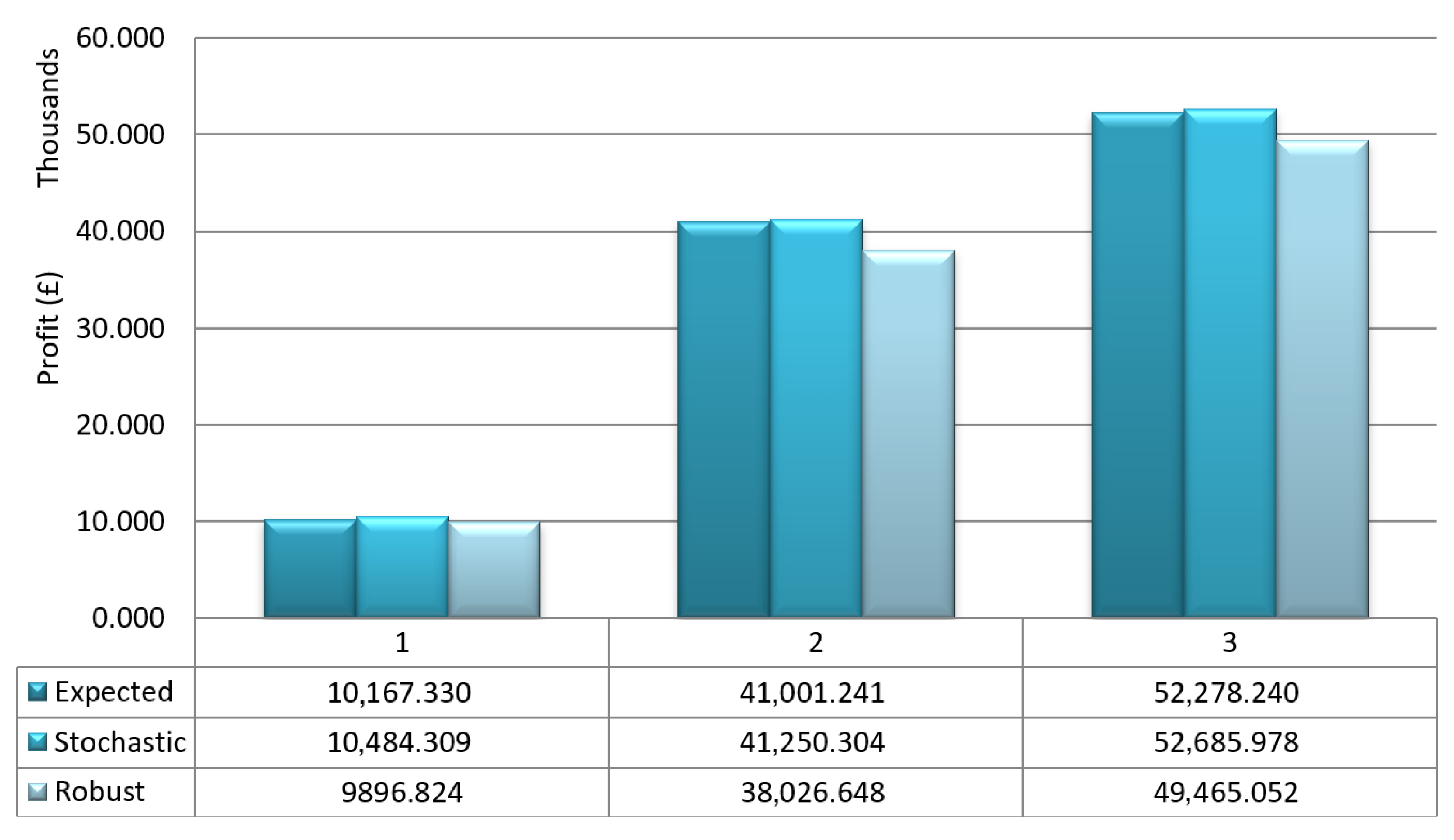
Figure 10.
Comparison of expectation-based offers for Case B1 and Case B2.
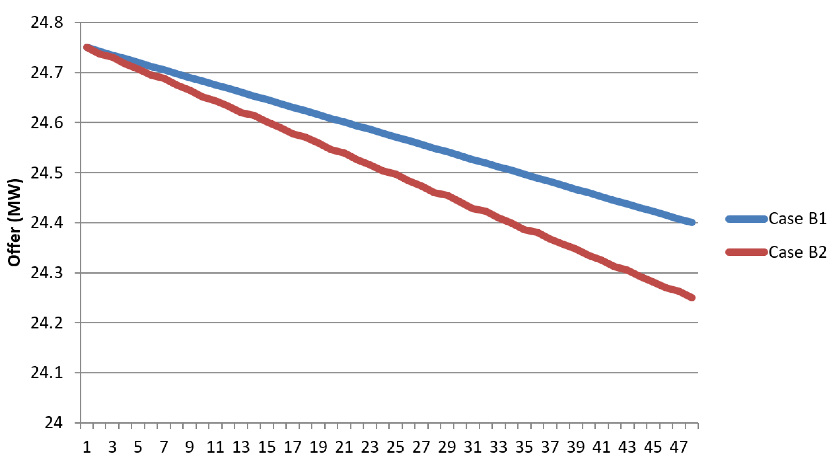
Figure 11.
Comparison of stochastic offers for Case B1 and Case B2.
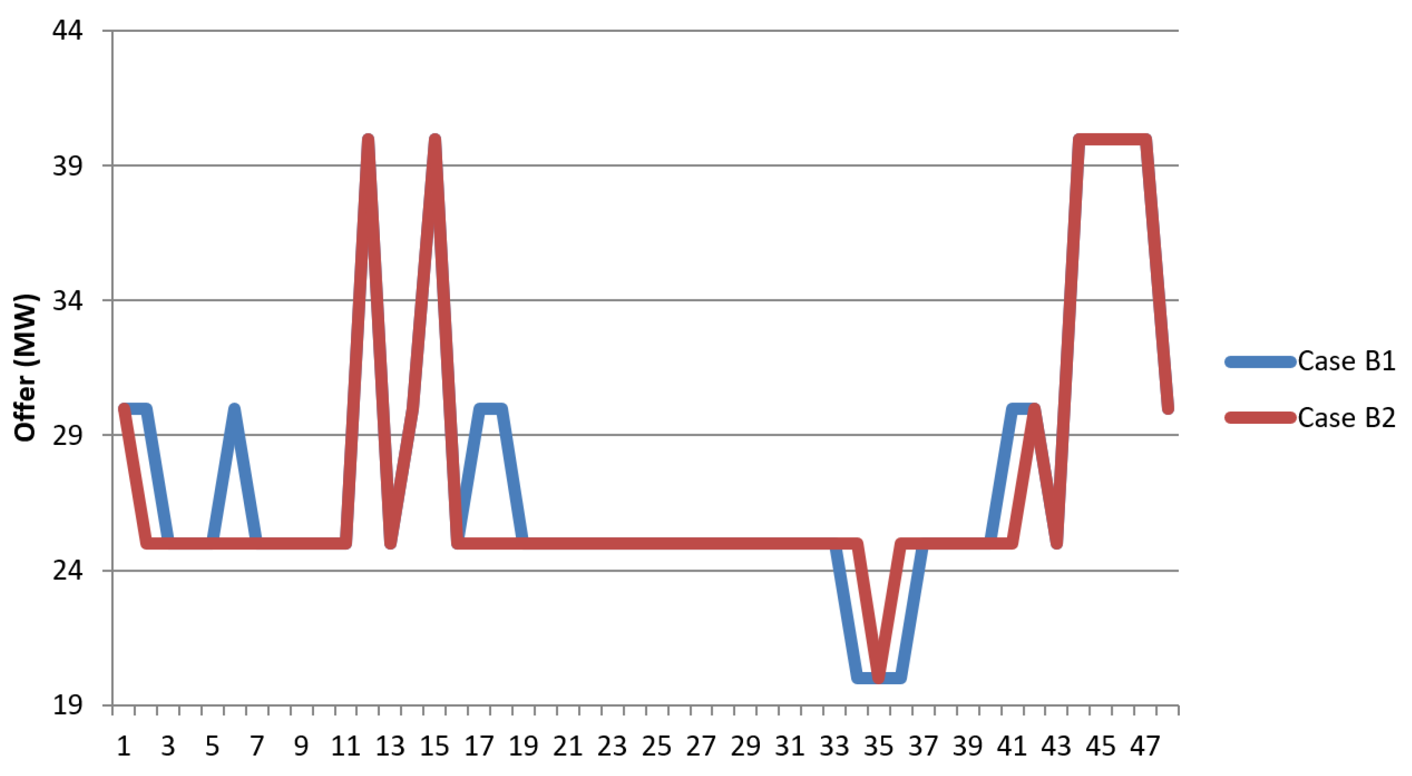
Figure 12.
Offered quantity for Case A.
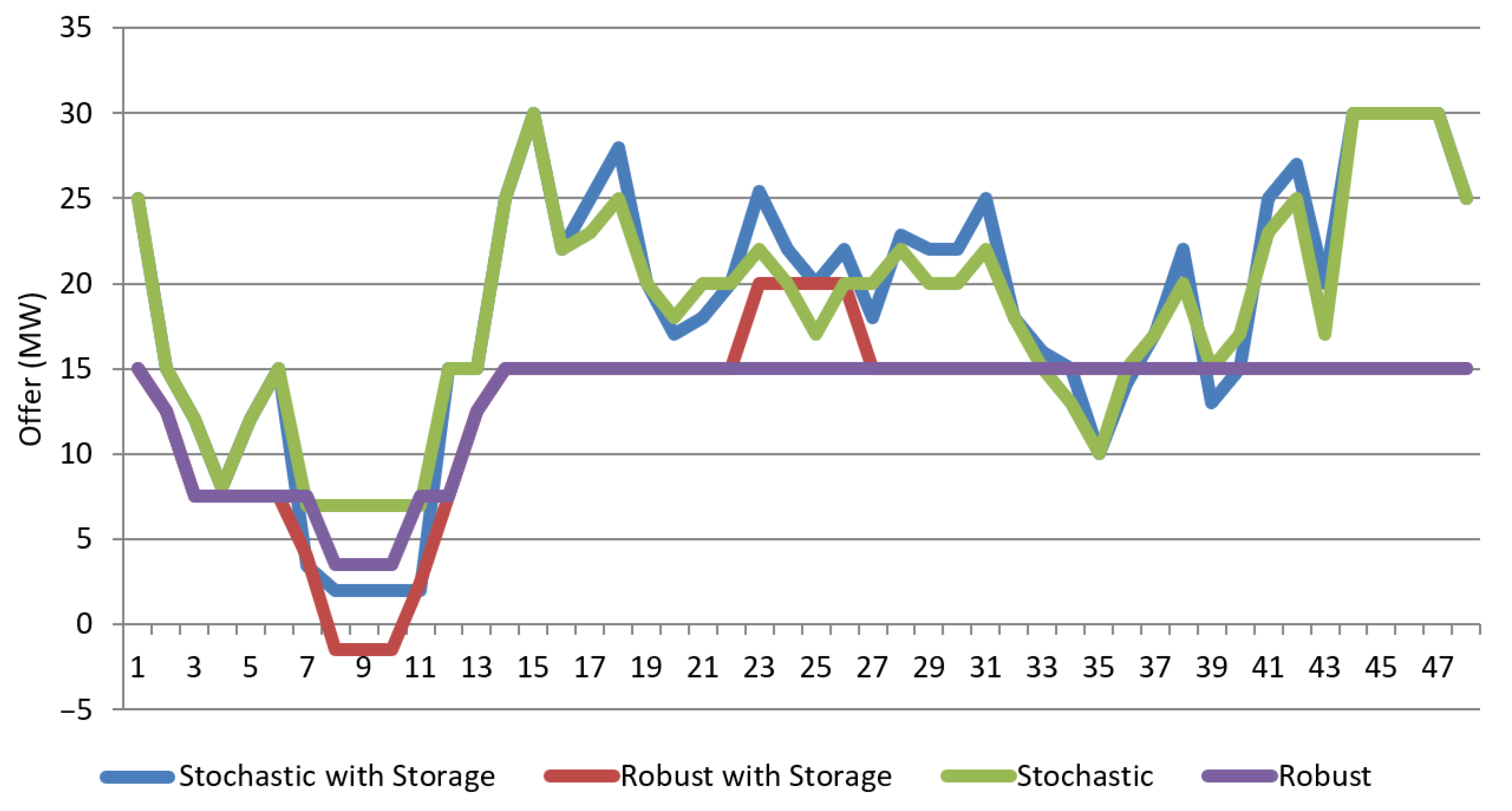
Figure 13.
Offered quantity for Case B.
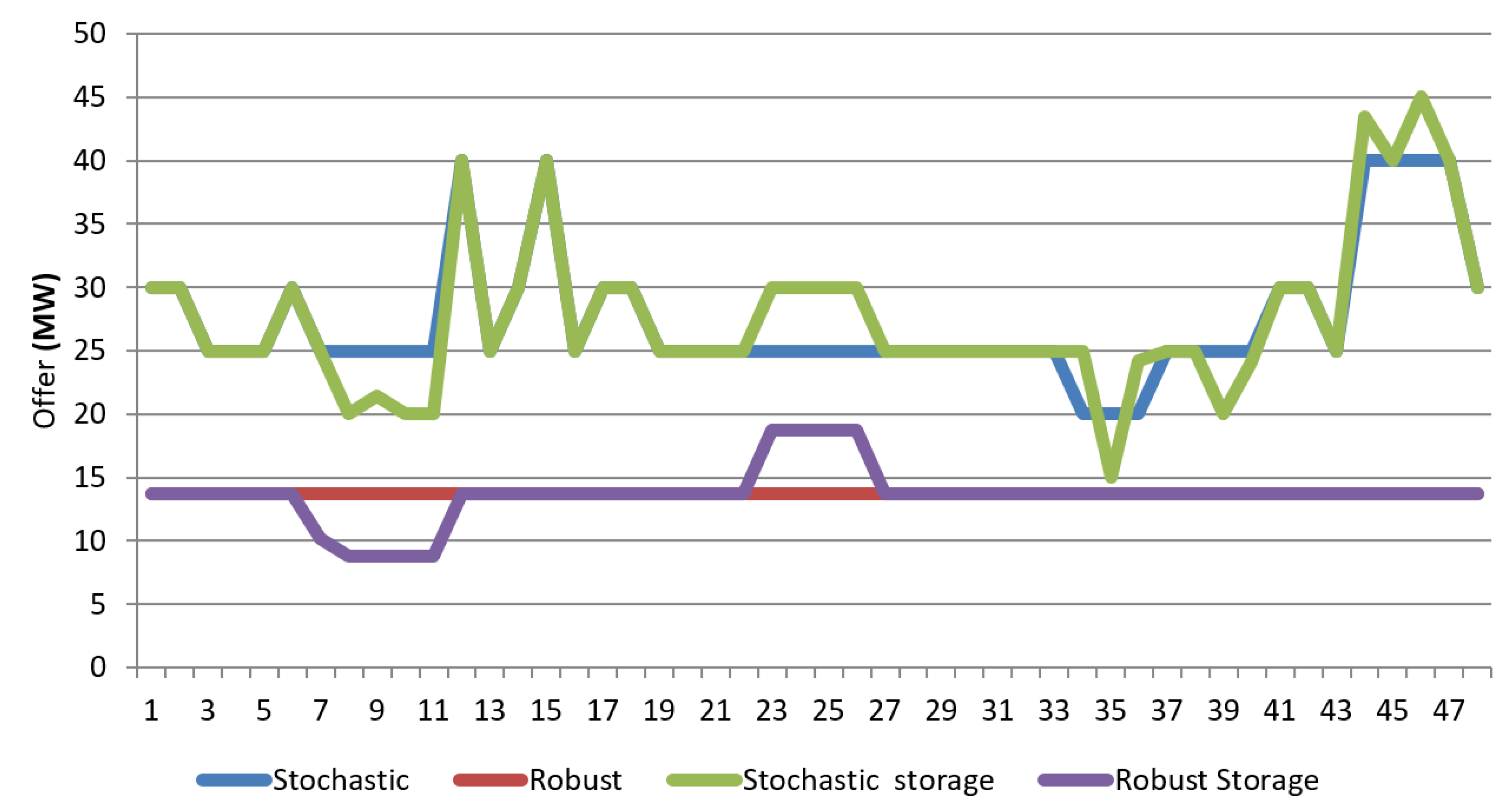
Figure 14.
Offered quantity for Case C.
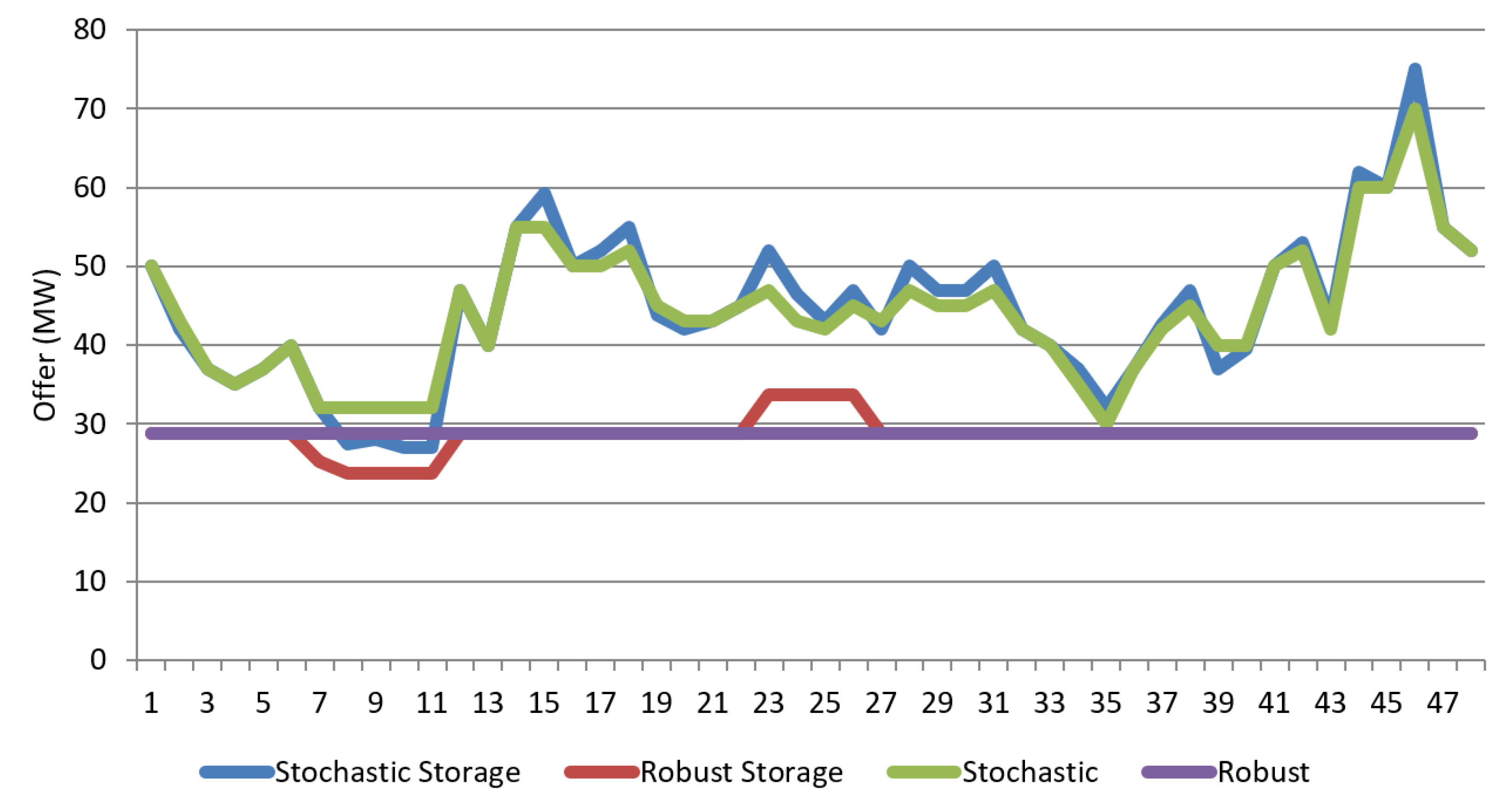
Figure 15.
Comparison of expected profits for different cases with storage constraints.
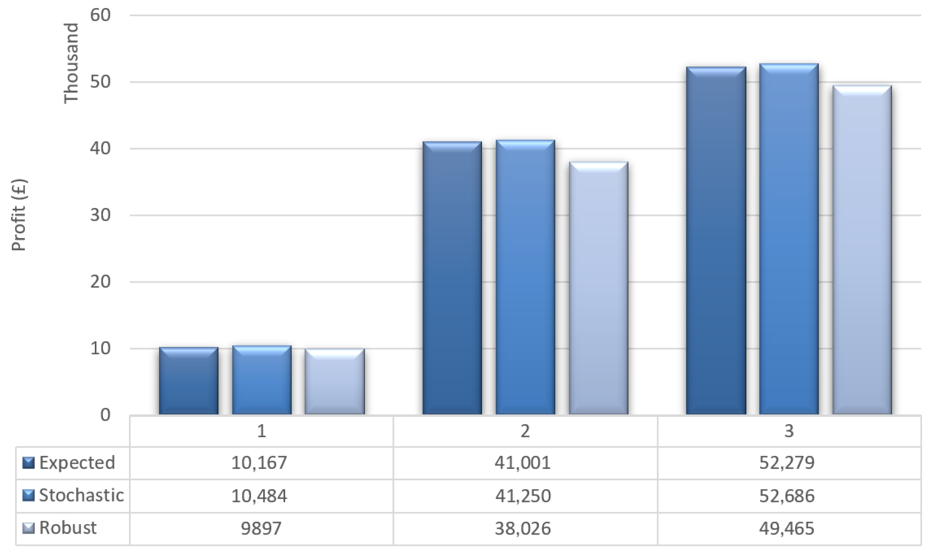
Figure 16.
Comparison of expected profits for different storage parameters for all optimisation methods—expectation-based (blue), stochastic (green), and robust (red).
Figure 16.
Comparison of expected profits for different storage parameters for all optimisation methods—expectation-based (blue), stochastic (green), and robust (red).
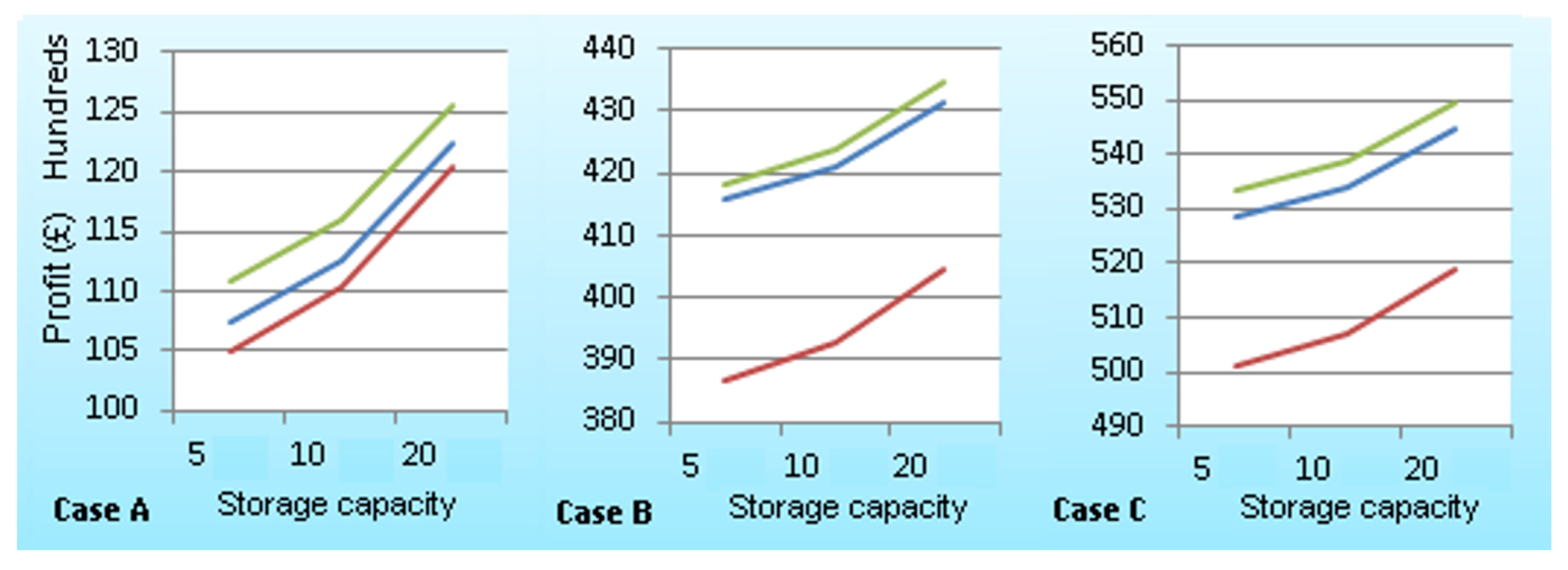
Figure 17.
Comparison of robust offers for different robustness levels.
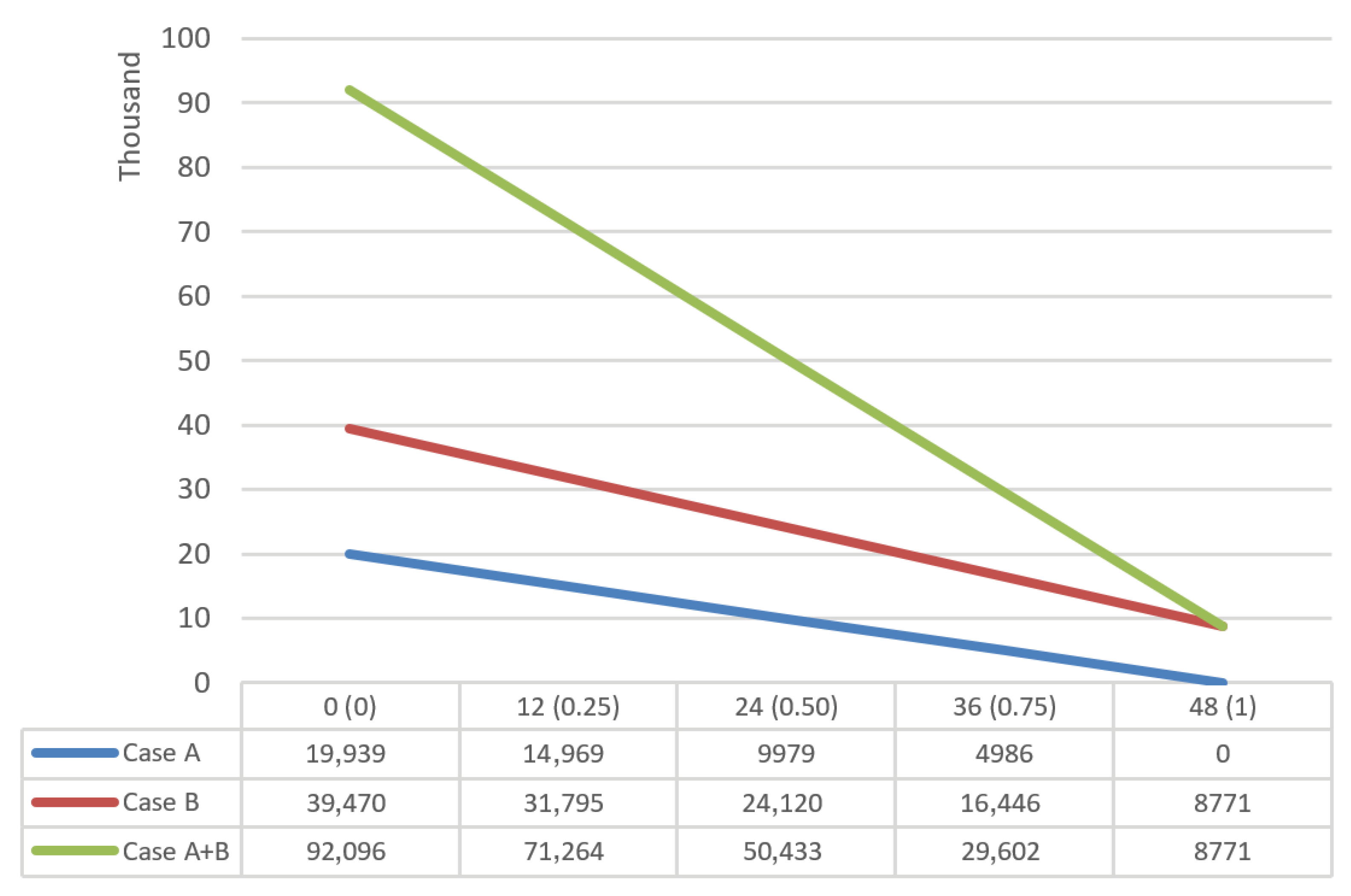

Table 1.
Battery storage parameters.
| Efficiency [p.u.] | Charging Power Limit [MW] | Discharging Power Limit [MW] | Maximum Charge [MWh] |
|---|---|---|---|
| 0.85 | 5 | 5 | 10 |
Table 2.
Input data for conventional generation.
| No. | Capacity [MW] | Gen. Cost [GBP/MWh] | Availability [p.u.] | Expected Capacity [MW] |
|---|---|---|---|---|
| CG1 | 5 | 50 | 0.65 | 3.25 |
| CG2 | 10 | 40 | 0.70 | 7.00 |
| CG3 | 8 | 45 | 0.55 | 4.40 |
| CG4 | 7 | 48 | 0.60 | 4.20 |
| Total | 30 | - | - | 18.85 |
Table 3.
Input data for wind generation.
| No. | Output [MW] | Initial Probability [p.u.] | Final Probability [p.u.] |
|---|---|---|---|
| WG1 | 5 | 0.05 | 0.12 |
| WG2 | 20 | 0.20 | 0.20 |
| WG3 | 25 | 0.50 | 0.36 |
| WG4 | 30 | 0.20 | 0.20 |
| WG5 | 40 | 0.05 | 0.12 |
Table 4.
Breakdown of the expected profit for all three offers (Case 1).
| Offer | Market Revenue (GBP) | Surplus Revenue (GBP) | Shortage Cost (GBP) | Generation Cost (GBP) | Profit (GBP) |
|---|---|---|---|---|---|
| Stochastic | 34,534 | 2764 | −8609 | −17,616 | 11,073 |
| Robust | 24,544 | 5293 | −2971 | −16,450 | 10,416 |
| Expectation | 30,901 | 2890 | −6005 | −17,032 | 10,755 |
Table 5.
Wind generator output and probability comparisons.
| Generator | Output [MW] | Initial Prob. [p.u.] | Final Prob. [p.u.] |
|---|---|---|---|
| WG1 | 5 | 0.05 | 0.12 |
| WG2 | 20 | 0.2 | 0.2 |
| WG3 | 25 | 0.5 | 0.36 |
| WG4 | 30 | 0.2 | 0.2 |
| WG5 | 40 | 0.05 | 0.12 |
| Generator | Output [MW] | Initial Prob. [p.u.] | Final Prob. [p.u.] |
| WG1 | 5 | 0.05 | 0.15 |
| WG2 | 20 | 0.1 | 0.1 |
| WG3 | 25 | 0.7 | 0.5 |
| WG4 | 30 | 0.1 | 0.1 |
| WG5 | 40 | 0.05 | 0.15 |
Table 6.
Financial analysis for various cases and scenarios.
| Scenario | Case A | Case B | Case C | |||
|---|---|---|---|---|---|---|
| Worst Case (£) | Best Case (£) | Worst Case (£) | Best Case (£) | Worst Case (£) | Best Case (£) | |
| Stochastic | −8596 | 49,192 | 66 | 72,601 | −833 | 94,124 |
| High, CG1 | High, CG16 | High, WG1 | High, WG5 | High, CG1, WG1 | High, CG16, WG5 | |
| Robust | −7151 | 45,695 | 5409 | 67,078 | −1980 | 86,971 |
| High, CG1 | High, CG16 | High, WG1 | High, WG5 | High, CG1, WG1 | High, CG16, WG5 | |
| Expectation-Based | −8848 | 21,083 | 95 | 71,469 | −8753 | 92,581 |
| High, CG1 | High, CG16 | High, WG1 | High, WG5 | High, CG1, WG1 | High, CG16, WG5 | |
Table 7.
Comparison of expected profits for different storage parameters.
| Scenario | Case A | Case B | Case A + B | ||||||
|---|---|---|---|---|---|---|---|---|---|
| C/D rate MW (Energy MWh) | 5 (10) | 10 (20) | 20 (40) | 5 (10) | 10 (20) | 20 (40) | 5 (10) | 10 (20) | 20 (40) |
| Expectation-Based | 10,733 | 11,259 | 12,243 | 41,575 | 42,111 | 43,155 | 52,862 | 53,419 | 54,477 |
| Stochastic | 11,076 | 11,596 | 12,548 | 4183 | 42,386 | 43,447 | 53,323 | 53,884 | 54,941 |
| Robust | 10,490 | 11,041 | 12,038 | 38,672 | 39,301 | 40,438 | 50,099 | 50,709 | 51,866 |
Table 8.
Aggregation benefits for different storage parameters.
| Capacity, MW (C/D Rate, MWh) | C-(A + B) | ||
|---|---|---|---|
| 5 (10) | 10 (20) | 20 (40) | |
| Expectation-Based | 554 | 50 | −921 |
| Stochastic | 414 | −98 | −1054 |
| Robust | 937 | 367 | −609 |
Disclaimer/Publisher’s Note: The statements, opinions and data contained in all publications are solely those of the individual author(s) and contributor(s) and not of MDPI and/or the editor(s). MDPI and/or the editor(s) disclaim responsibility for any injury to people or property resulting from any ideas, methods, instructions or products referred to in the content. |
© 2025 by the authors. Licensee MDPI, Basel, Switzerland. This article is an open access article distributed under the terms and conditions of the Creative Commons Attribution (CC BY) license.
Copyright: This open access article is published under a Creative Commons CC BY 4.0 license, which permit the free download, distribution, and reuse, provided that the author and preprint are cited in any reuse.


