
Submitted:
25 February 2026
Posted:
26 February 2026
You are already at the latest version
Abstract
Purpose: To develop a fully automated 2D nnU-Net pipeline for multi-class skeletal muscle segmentation (psoas, paraspinal, and abdominal wall) at the third lumbar (L3) vertebral level, and to quantitatively evaluate its diagnostic performance and reliability compared to manual segmentation.
Materials and Methods: A 2D nnU‑Net was trained on 164 axial L3 CT slices from the multi-institutional AMOS22 dataset, spanning diverse abdominal pathologies and multivendor imaging. To assess generalizability under severe anatomical distortion, independent external validation was performed in 50 consecutive patients with advanced liver disease from a single institution (January–December 2025; mean age, 63 ± 15 years; 32 women, 18 men), of whom 88% had moderate-to-severe ascites. Model stability was examined by comparing a five‑fold ensemble with the best‑performing single‑fold model. Intra‑observer reliability of the manual reference standard was evaluated in a random subset of 30 cases. Performance metrics included the Dice Similarity Coefficient (DSC), Pearson correlation coefficient (r), and Bland–Altman analysis for cross‑sectional areas and mean attenuation. The inference workflow was deployed via a custom Streamlit‑based graphical user interface (GUI).
Results: In this anatomically complex external validation cohort, the 5-fold ensemble 2D nnU-Net achieved an overall mean DSC of 0.937 ± 0.043, with 80% of cases achieving a mean DSC ≥ 0.90. While the mean DSC was statistically comparable to the best single-fold model (0.937, p = 0.736), the ensemble strategy increased the minimum observed DSC (worst-case performance) from 0.720 to 0.822. Comparison between the ensemble model and manual segmentation yielded a Pearson correlation of r = 0.955 (p < 0.001) for total skeletal muscle area, with a mean bias of +7.17 cm². Intra-observer agreement for the manual reference standard demonstrated a correlation of r = 0.995 for total area. The automated pipeline required 3-5 seconds per case for inference and quantitative reporting, compared to 3-5 minutes for manual segmentation.
Conclusion: In patients with advanced liver disease and substantial anatomical distortion from ascites, an ensemble-based 2D nnU‑Net provides quantitative accuracy and measurement agreement comparable to manual L3 skeletal muscle segmentation, while mitigating lower-bound (worst-case) errors relative to single-fold models. Integration with a dedicated GUI enables substantial time savings and supports scalable clinical body composition analysis.
Keywords:
sarcopenia
; skeletal muscle segmentation
; computed tomography
; deep learning
; liver cirrhosis
1. Introduction
Sarcopenia, a term initially proposed by Irwin H. Rosenberg to describe age-related muscle loss, has become a critical focal point across diverse medical disciplines [1]. The European Working Group on Sarcopenia in Older People (EWGSOP) formally defines sarcopenia as a syndrome characterized by the generalized and progressive loss of skeletal muscle mass and strength, which is associated with adverse outcomes, including reduced quality of life and increased mortality [2,3,4,5,6,7,8]. While sarcopenia is estimated to affect 5 to 10% of the population over the age of 65 years in the context of primary geriatric frailty, opportunistic body composition analysis has demonstrated its broader clinical significance [2,9,10,11,12,13,14]. Reduced skeletal muscle mass is now recognized as an independent predictor of adverse clinical outcomes across diverse patient populations, leading to increased rates of surgical complications, higher chemotherapy toxicity, prolonged hospital length of stay, and decreased overall survival in patients with malignancies, end-stage liver disease, and major vascular conditions [15,16,17,18,19,20,21,22,23].
The quantitative assessment of sarcopenia is most commonly performed using cross-sectional imaging, specifically computed tomography (CT) [16,17,24,25,26,27,28,29]. The skeletal muscle cross-sectional area (SMA) measured at the level of the third lumbar vertebra (L3) serves as the established reference standard, as it exhibits a high linear correlation with total body skeletal muscle volume [3,12,26,30,31,32,33]. At this anatomical landmark, the target musculature comprises three distinct groups: the psoas, the paraspinal (erector spinae and quadratus lumborum), and the abdominal wall muscles (transversus abdominis, internal and external obliques, and rectus abdominis) [26,31,33,34]. Despite the proven prognostic value of L3 skeletal muscle quantification, its integration into routine clinical practice remains limited by methodological bottlenecks [4,5,35]. The current reference standard for extracting these metrics relies on manual or semi-automated segmentation using third-party analytical software (e.g., Slice-O-Matic, ImageJ, or Horos) [36,37,38]. These conventional tools primarily utilize Hounsfield Unit (HU) thresholding—typically applying a predefined window of -29 to +150 HU—to isolate skeletal muscle from surrounding adipose tissue and viscera [4,27].
While HU thresholding is effective in healthy anatomies, it frequently fails in complex clinical scenarios [39,40]. In patients with sarcopenia, the abdominal wall muscles often become severely thinned and undergo myosteatosis (fatty infiltration), which alters their radiodensity [26,33,34,41]. Furthermore, the presence of abdominal wall edema, ascites, or closely apposed bowel loops creates anatomical interfaces with attenuation values that overlap those of skeletal muscle [39,42,43]. In these instances, thresholding algorithms cannot accurately delineate the peritoneal boundary, necessitating extensive manual correction by a human reader [39]. This manual tracing process is highly labor-intensive, often requiring 3 to 5 minutes per axial slice, thereby introducing inter-observer variability and precluding large-scale, population-level opportunistic screening [44,45,46]. To address the limitations of manual segmentation, deep learning (DL) algorithms, particularly convolutional neural networks (CNN) based on the U-Net architecture, have been increasingly applied to medical image segmentation [35,44,45,46,47,48]. The nnU-Net framework, a self-configuring architecture, currently represents the state of the art for such tasks, automating hyperparameter tuning and preprocessing to achieve high spatial accuracy [49,50,51,52,53].
However, translating these high-performing theoretical models into reliable clinical tools presents ongoing challenges [54,55,56]. A review of current literature indicates that many published DL models for body composition are trained and validated on relatively homogenous, single-center datasets or heavily index toward healthy outpatient populations [39,45,47,57,58]. When deployed on external datasets containing high-acuity pathologies—such as massive tumors, postoperative anatomical distortion, or severe fluid shifts—these models are susceptible to severe segmentation failures [40,45,59,60]. In a clinical quality and safety context, these unpredictable lower-bound errors limit the trustworthiness of fully automated pipelines [60,61]. Most existing DL approaches utilize a single-fold model architecture, which lacks a consensus mechanism to resolve anatomical ambiguity at the muscle-peritoneum interface [49,62,63].
To bridge the gap between technical DL performance and safe clinical deployment, robust segmentation pipelines must be validated on complex, multi-vendor clinical data. Furthermore, to achieve efficient workflow integration, these technical pipelines must be accessible through intuitive software interfaces. Therefore, this study was initiated to develop and independently validate a fully automated 2D nnU-Net pipeline for L3 skeletal muscle segmentation. To maximize model generalizability, the training phase utilized a heterogeneous, multi-institutional dataset containing diverse abdominal pathologies. Additionally, to rigorously test algorithmic stability under severe anatomical distortions, external validation was conducted on a challenging clinical cohort of patients with advanced liver disease. To address unpredictable segmentation failures, we implemented a 5-fold ensemble inference strategy to stabilize boundary predictions. Finally, we integrated this ensemble model into a custom graphical user interface (GUI) to evaluate its impact on measurement reliability and workflow efficiency compared to the conventional manual reference standard.
2. Materials and Methods
2.1. Study Design and Patient Cohorts
This retrospective study used two distinct datasets for model development and independent external validation. For model training and internal cross-validation, 164 axial CT slices at the L3 vertebral level were extracted from the AMOS22 (Abdominal Multi-Organ Segmentation) dataset, a multi-institutional, multivendor resource. Metadata analysis of the training pool showed a diverse distribution of scanner manufacturers (Toshiba, Siemens, GE, and Philips) and a mean patient age of 53.7 ± 16.3 years. To promote robustness to anatomical distortion, we purposefully selected cases representing a heterogeneous spectrum of abdominal pathologies, including ascites, primary and metastatic hepatic malignancies, renal tumors, and peritoneal carcinomatosis.
The independent external validation cohort (n = 50) was retrospectively identified from an existing Institutional Review Board–approved study evaluating predictors of transjugular intrahepatic portosystemic shunt (TIPS) revision in patients with advanced liver disease (Table 1). As a result, clinical indications for imaging were clustered around chronic hepatic pathology; the most common were liver cirrhosis (22%), routine TIPS evaluation (20%), and refractory ascites (18%). From an algorithmic perspective, this cohort was designed to stress-test the segmentation pipeline: patients with end-stage liver disease frequently exhibit compounding anatomical distortions—severe macroscopic sarcopenia, massive ascites, subcutaneous abdominal edema, and altered fascial planes—that pose challenging edge cases for both manual tracing and automated boundary delineation.
Exclusion criteria for the external validation cohort were:
- CT examinations in which the L3 axial slice did not encompass complete abdominal coverage,
- DICOM studies that could not be exported due to PACS technical issues,
- Absence of abdominal CT (abdominal MRI only), and
- Ineligibility related to the source database (patients who did not undergo a TIPS procedure).
2.2. Image Preprocessing and Reference Standard Generation
To mitigate inter-reader variability and standardize the segmentation workflow, a custom GUI was developed using the Streamlit framework (version 1.30.0, https://streamlit.io/) in Python. All L3 axial CT images were loaded into the GUI and preprocessed using a standard soft-tissue window (window width: 400 HU; window level: 50 HU) to optimize the visualization of muscle-adipose interfaces. A board-certified radiologist (HY) generated manual reference standards utilizing a custom brush-based annotation interface within the Streamlit application. Three distinct target classes were sequentially delineated and consolidated into a unified label map: the psoas muscle (class 1), the paraspinal muscles (class 2), and the abdominal wall muscles (class 3), with the background designated as class 0.
Upon completion of each case, the application automatically exported and archived the original CT slice and the corresponding final label map as a pair of Neuroimaging Informatics Technology Initiative (NIfTI) files (*-image.nii.gz and *-label.nii.gz). This standardized nomenclature and label identification protocol ensured direct compatibility for subsequent dataset curation and model training. Concurrent with mask generation, case-level quantitative logs—including total and class-specific cross-sectional area (cm²), mean attenuation (HU), and attenuation standard deviation—were extracted to serve as the reference standard.
To establish the stability of this manual reference standard and mitigate recall bias, intra-observer reliability was quantitatively assessed. The same board-certified radiologist performed a second, independent manual segmentation round on a random subset of 30 cases from the initial AMOS22 training dataset. This second annotation session was conducted after a minimum 14-day washout period, and the rater was strictly blinded to the initial segmentation results and clinical metadata.
2.3. Model Architecture and Training Protocol
An automated segmentation model was developed using the 2D configuration of the nnU-Net v2 framework. The nnU-Net utilizes a self-configuring U-Net encoder-decoder architecture that automatically dynamically adapts image preprocessing, network topology, and training hyperparameters based on the heuristic properties of the training dataset.
Model training was executed on a local workstation equipped with an NVIDIA GeForce RTX 4090 graphics processing unit (24 GB VRAM). Training was conducted using a 5-fold cross-validation strategy. To implement this, the 164-case training dataset was partitioned into five non-overlapping subsets (folds). The network was trained five times; in each iteration, four folds (80% of the data) were used for active training, while the remaining fold (20%) was held out for internal validation.
This rotational sampling ensures that every image in the dataset is used exactly once as unseen validation data, thereby mitigating the risk of overfitting and providing a robust, unbiased estimate of internal segmentation accuracy. Each fold was trained for 1,000 epochs, requiring an average computational time of 7.3 to 7.7 hours per fold (average epoch duration of approximately 26 seconds).
The network was optimized using a batch size of 6, an image patch size of 640 x 640 pixels, and a resampled in-plane voxel spacing of 0.782 x 0.782 mm. Image intensities were standardized utilizing the framework’s dedicated CT normalization scheme (CTNormalization), which automatically clips Hounsfield Unit (HU) values based on the global foreground statistics of the training cohort. Standardized data augmentation techniques, including random rotations, scaling, and Gaussian noise addition, were applied during training to enhance the model’s resilience to variations in scanner protocols and image reconstruction algorithms.
Following the cross-validation phase, an ensemble inference strategy was employed to process the external validation cohort. Instead of relying on a single network hierarchy, the output probability maps generated by all five independently trained folds were mathematically averaged. This approach subsequently yielded a final, stable label map for each unseen clinical case, thereby mitigating the risk of localized boundary failures associated with single-model predictions.
2.4. Automated Inference Workflow and User Interface
To facilitate clinical evaluation and streamline future dataset curation, the trained 2D nnU-Net models were deployed within the local Streamlit application. This end-to-end clinical workflow consists of four primary functions: (1) direct importation of unannotated single-slice CT images; (2) manual multi-class segmentation with brush-based editing capabilities; (3) on-demand execution of automated 2D nnU-Net inference, allowing the user to select either the best-performing single-fold network or the 5-fold ensemble architecture to generate initial predictive or comparison masks; and (4) real-time review of quantitative outputs. During model testing, the application automatically computes spatial overlap metrics when a reference mask is present, alongside immediate area and attenuation summaries. For each completed case, the application exports the original image and final label map as a paired NIfTI set (*-image.nii.gz, *-label.nii.gz) with consistent naming and label IDs, enabling direct reuse of outputs for dataset curation and iterative model testing.
2.5. Statistical Analysis
Quantitative evaluation of spatial overlap between the automated segmentations and the manual reference standard was performed using the Dice Score and Dice Similarity Coefficient (DSC). The Dice Score between the predicted mask and the reference mask was defined as:
where represents the predicted segmentation, represents the manual ground truth, denotes the number of voxels shared by both masks, and and correspond to the number of voxels labeled positive in the predicted and manual masks, respectively.
The equivalent formulation in terms of classification performance was also computed:
where , , and indicate the number of true-positive, false-positive, and false-negative voxels, respectively. Performance was analyzed for each individual muscle class as well as the overall mean across all foreground classes.
Clinical utility was assessed by extracting the total cross-sectional area (cm²) and mean attenuation (HU) from the generated label maps. The agreement between the 2D nnU-Net measurements and the manual reference measurements was evaluated using the Pearson correlation coefficient (r) and Mean Absolute Error (MAE). Bland-Altman analysis was conducted to determine the mean bias and the 95% limits of agreement between the two methods.
To quantify the benefit of the ensemble architecture, a paired t-test was used to compare the mean DSC of the 5-fold ensemble model with that of the single best-performing fold from the cross-validation phase. Statistical significance was defined as a p-value < 0.05.
Quantitative metrics were extracted from NIfTI label maps using custom Python scripts, employing the nibabel library (version 5.3.2) for medical image input/output and numpy (version 2.4.2) for numerical array operations. All subsequent tabular data aggregation and statistical analyses were conducted utilizing pandas (version 2.2.3) and scipy.stats module within the scipy library (version 1.17.0). Graphical visualizations, including box plots, correlation plots, and Bland-Altman plots, were generated using the matplotlib (version 3.9.1) and seaborn (version 0.13.2) libraries.
3. Results
3.1. Internal Cross-Validation Performance
During the initial development phase, the 2D nnU-Net model demonstrated high internal consistency across the 164-case training cohort. In the 5-fold cross-validation, the overall mean foreground Dice similarity coefficient (DSC) was 0.931 ± 0.010 (Table 2). Spatial overlap was highest for the paraspinal muscle group (DSC: 0.948 ± 0.010), followed by the psoas muscles (DSC: 0.937 ± 0.008), and the anatomically complex abdominal wall muscles (DSC: 0.908 ± 0.012). These internal validation metrics established a robust baseline for subsequent external testing (Figure 1).
3.2. External Validation and Ensemble Efficacy
Independent external validation was conducted on the 50-case clinical cohort. The 5-fold ensemble 2D nnU-Net model achieved an overall mean DSC of 0.937 ± 0.043 across all muscle classes, demonstrating high generalizability to multi-vendor, unseen data (Figure 2). Performance remained stratified by anatomical complexity: paraspinal DSC was 0.960, psoas DSC was 0.941, and abdominal wall DSC was 0.911 (Table 3).
To evaluate the utility of the ensemble architecture, performance was compared against the single best-performing fold from the internal validation phase (Fold 4). While the overall mean DSC between the best single fold and the 5-fold ensemble was statistically comparable (0.937 vs. 0.937, p = 0.736), the ensemble strategy demonstrated a measurable impact on segmentation stability in challenging cases (Table 3). Specifically, the ensemble approach increased the minimum observed DSC within the cohort—representing the “worst-case” segmentation—from 0.720 (single fold) to 0.822 (ensemble).
To further characterize the clinical reliability of the automated pipeline, the proportion of cases achieving a high-performance threshold (DSC ≥ 0.90) was evaluated. For the 5-fold ensemble model, 80% (40/50) of cases achieved an overall mean DSC ≥ 0.90 (sub-threshold mean: 0.868, n=10). At the class level, performance was most robust in the paraspinal musculature, where 98% (49/50) of cases exceeded the threshold; the single sub-threshold case maintained a high baseline DSC of 0.893. The psoas group achieved a DSC ≥ 0.90 in 84% (42/50) of cases (sub-threshold mean: 0.857, n=8). The abdominal wall presented the greatest anatomical challenge, exceeding the 0.90 threshold in 68% (34/50) of cases, though the 16 sub-threshold cases still maintained a clinically acceptable mean DSC of 0.836.
3.3. Clinical Agreement and Bias Analysis
Quantitative clinical metrics derived from the ensemble 2D nnU-Net predictions were compared against the manual reference standard. For total skeletal muscle cross-sectional area, Pearson correlation analysis demonstrated high agreement (r = 0.955, p < 0.001) with a mean absolute error (MAE) of 8.00 cm² (Table 4) (Figure 3). Bland-Altman analysis for total muscle area revealed a mean bias of +7.17 cm² (2D nnU-Net minus Manual), indicating a systematic, marginal increase in area quantification by the automated pipeline compared to the human rater (Figure 4).
Analysis of mean muscle attenuation (Hounsfield Units) also yielded high agreement between the automated model and the manual reference (r = 0.968), with an MAE of 2.33 HU and a minimal mean bias of -1.67 HU (Figure 5).
3.4. Intra-Observer Reliability and Time Efficiency
The stability of the manual reference standard was confirmed via intra-observer analysis on a random subset of 30 cases. Agreement between the two independent rounds of manual segmentation, separated by the 14-day washout period, demonstrated a consistency for total muscle area (r = 0.995, p < 0.001) (Figure 6), with an MAE of 1.98 cm² and a mean bias of -1.31 cm² (Table 5) (Figure 7).
Regarding workflow efficiency, the manual segmentation process required 3 to 5 minutes of active human interaction per axial slice. In contrast, the automated 2D nnU-Net pipeline, executed via the custom Streamlit GUI, performed end-to-end inference, label map generation, and quantitative metric extraction in 3-5 seconds per case.
3.5. Qualitative Assessment and Error Analysis
Visual inspection of the generated label maps aligned with the quantitative findings. In standard cross-sectional anatomies, the ensemble model demonstrated high anatomical fidelity, accurately delineating all three muscle compartments without encroaching on adjacent viscera (Figure 8).
However, a qualitative review of subthreshold cases in the advanced liver disease cohort revealed specific patterns of anatomical ambiguity. In non-contrast scans of patients with severe ascites, localized boundary failures occurred due to the inclusion of isodense structures, such as the kidney or adjacent peritoneum (Figure 9). Furthermore, profound subcutaneous edema occasionally altered normal soft-tissue density gradients, leading to localized over-segmentation of edematous tissue or under-segmentation of the oblique musculature (Figure 10).
4. Discussion
This study demonstrates that a fully automated, ensemble-based 2D nnU-Net pipeline can achieve high quantitative accuracy and clinical reliability for L3 skeletal muscle segmentation. Validated against a highly stable, expert-derived reference standard (intra-observer r = 0.995), the ensemble model demonstrated high spatial overlap (mean DSC 0.937) and measurement agreement (r = 0.955 for total area) on a diverse, high-acuity external clinical cohort. Crucially, the implementation of a 5-fold ensemble inference strategy provided a measurable fail-safe in anatomically complex cases, significantly raising the minimum performance threshold compared to single-fold architectures.
A notable finding of this study is the high generalizability of the ensemble model, which was trained on a relatively constrained cohort of 164 cases and successfully validated on a highly complex external cohort. In deep learning, model robustness is traditionally associated with large-scale datasets comprising thousands of annotated studies. However, our results demonstrate that the quantity of raw data can be effectively offset by dataset heterogeneity and an optimized network architecture. The selected AMOS22 training pool exhibited broad pathological diversity and technical variance across four distinct scanner manufacturers. By employing extensive, dynamic data augmentation during training, the nnU-Net framework forces the network to learn fundamental anatomical features rather than overfitting scanner-specific artifacts [49].
The efficacy of this training strategy was explicitly demonstrated in the external validation cohort, which comprised patients with advanced liver disease. A recent meta-analysis reported a pooled DSC of 0.941 for AI-based skeletal muscle segmentation across various studies [58]. While several contemporary deep learning models report higher spatial overlap metrics—such as DSCs of 0.97—these architectures are predominantly trained and validated on routine health check-up populations or general outpatients [64,65]. When automated pipelines are deployed on anatomically complex or diseased cohorts, performance predictably degrades. For instance, a previous U-Net model demonstrated a muscle DSC of 0.96 on a standard test set, which subsequently dropped to 0.92 when applied to a hepatocellular carcinoma cohort [39]. The external validation cohort in the present study, burdened by massive fluid shifts and profound soft-tissue edema, served as an intentional ‘stress test.’ By maintaining an overall mean DSC of 0.937 across unpredictable anatomical presentations (Figure 8), the 5-fold ensemble model demonstrates resilience against catastrophic boundary failures, proving its deployability in high-acuity clinical scenarios.
A critical objective of this study was to define the technical boundaries of the 2D nnU-Net. While the ensemble model achieved high average accuracy, threshold analysis (DSC ≥ 0.90) revealed distinct, class-specific anatomical vulnerabilities. The paraspinal musculature demonstrated high algorithmic resilience (98% of cases ≥ 0.90), likely because it is spatially anchored by rigid osseous landmarks (the vertebral body and transverse processes) that remain identifiable despite soft-tissue distortion. Conversely, the abdominal wall proved the most challenging target, falling below the 0.90 threshold in 32% of cases. This class-specific performance gradient is corroborated by previous body composition studies, which consistently identify the anterolateral abdominal wall as the most anatomically vulnerable compartment due to its natively thin muscular composition, highly variable fascial boundaries, and susceptibility to severe myosteatosis [45].
Qualitative analysis of sub-optimal predictions (Figure 9) indicates that these relative failures are rarely arbitrary; rather, they are driven by severe, patient-specific pathological alterations. In patients with profound sarcopenia, the rectus abdominis and oblique muscles become extremely thin, causing the automated boundary to inadvertently capture adjacent peritoneal layers. Similarly, severe subcutaneous edema disrupts normal tissue gradients, prompting the algorithm to over-segment into the infiltrated adipose tissue (Figure 10). The psoas muscle exhibited localized vulnerabilities (16% of cases < 0.90) primarily on unenhanced imaging, particularly when combined with third-spacing fluid. As demonstrated in Figure 9, the presence of ascites on non-contrast CT renders the left psoas completely isodense with the adjacent left kidney, leading to a false-positive algorithmic bridging between the structures.
Despite these complex localized failures, the sub-threshold cases for the abdominal wall and psoas still maintained mean DSCs of 0.836 and 0.857, respectively, proving that the ensemble architecture reliably prevents catastrophic, whole-image segmentation collapse even in severely distorted anatomies. Bland-Altman analysis revealed a systematic positive mean bias of 7.17 cm² in total muscle area when comparing the ensemble model with the manual reference. In the context of cross-sectional macroscopic anatomy, this marginal overestimation is a positive indicator of algorithmic consistency. The 2D nnU-Net reliably includes thin fascial planes and muscle-peritoneum interfaces that a human rater—acting with necessary caution to avoid inadvertently including visceral fat or bowel—might conservatively omit during manual tracing. This finding aligns with validation studies of fully automated body composition pipelines, which frequently report a high correlation combined with a slight positive volumetric bias, reflecting the AI’s persistent inclusion of intermuscular tissue that human readers tend to under-segment [48].
The transition from conventional semi-automated thresholding to this fully automated DL pipeline addresses the primary bottleneck in body composition research. Threshold-based tools require extensive manual correction when HU values are distorted by myosteatosis or adjacent pathology. By providing a semantic understanding of the anatomy, the 2D nnU-Net distinguishes between adjacent structures regardless of HU overlap. Integrated into a custom Streamlit GUI, this pipeline reduced the time required for complete segmentation, metric extraction, and reporting from 3 to 5 minutes to merely 3 to 5 seconds per case. This processing speed strictly aligns with the performance of recently implemented fully automated AI screening systems, which report mean processing times of approximately 4 seconds from CT acquisition to final report generation [65]. This magnitude of efficiency gain is a prerequisite for transitioning sarcopenia evaluation from a niche research endeavor to routine, population-level opportunistic screening.
This study has several limitations. First, despite a multi-institutional training source, the sample size—164 training slices and 50 external validation cases—is modest relative to population-scale DL studies with thousands of annotated exams [64]. Although augmentation and an ensemble strategy improved performance, generalizability should be confirmed in larger, multicenter, high-acuity cohorts. Second, the external validation cohort was intentionally enriched for advanced liver disease to stress-test performance under severe anatomical distortion (e.g., ascites, edema), introducing spectrum bias and limiting applicability to routine opportunistic screening. Future validation should include broader clinical indications, disease severities, and body habitus across institutions. Third, the pipeline operates on a single 2D axial L3 slice. While L3 is a validated surrogate for whole-body muscle mass, single-slice analysis is an approximation and sensitive to inter-individual anatomic variability; 3D volumetric and/or multi-slice approaches merit evaluation [48]. Fourth, reported processing times for manual versus automated workflows are observational estimates rather than outputs of a formal time–motion study; prospective measurement should quantify mean time savings, variability, and cost/throughput effects in high-volume settings. Finally, the retrospective, single-institution design limits inferences about effects on clinical decision-making and patient outcomes. Prospective deployment studies are needed to assess real-time impact and patient-centered outcomes.
5. Conclusions
The developed ensemble-based 2D nnU-Net pipeline provides an accurate, reliable, and time-efficient solution for L3 skeletal muscle segmentation. By training on a heterogeneous dataset and employing a 5-fold ensemble strategy, the model effectively mitigates catastrophic segmentation failures in anatomically complex patients. Integrated with a custom GUI, this automated tool eliminates the labor-intensive bottlenecks of manual segmentation, enabling the scalable, opportunistic assessment of sarcopenia and body composition in routine clinical practice.
Funding
This research received no external funding.
Institutional Review Board Statement
The study was conducted in accordance with the Declaration of Helsinki and was approved by the Institutional Review Board (IRB) of the UNC School of Medicine (protocol 25-2145).
Informed Consent Statement
The IRB waived the requirement for informed consent because no direct patient contact occurred.
Data Availability Statement
The AMOS22 multi-institutional dataset used for model training is publicly available at: https://amos22.grand-challenge.org/. The custom Streamlit application template for image annotation, end-to-end model inference, and quantitative reporting is open source at: https://github.com/hyeonyu-IR/segmentation-label-app. Patient-level segmentation data generated from institutional CT studies for external validation are available from the corresponding author upon reasonable request, but are not publicly shared due to privacy and institutional ethical restrictions.
Conflicts of Interest
The author declares no conflicts of interest.
References
- Rosenberg, I.H. Sarcopenia: origins and clinical relevance. J Nutr 1997, 127, 990S–1S. [Google Scholar] [CrossRef] [PubMed]
- Ribeiro, S.M.; Kehayias, J.J. Sarcopenia and the analysis of body composition. Adv Nutr 2014, 5, 260–267. [Google Scholar] [CrossRef] [PubMed]
- Derstine, B.A.; Holcombe, S.A.; Ross, B.E.; Wang, N.C.; Su, G.L.; Wang, S.C. Skeletal muscle cutoff values for sarcopenia diagnosis using T10 to L5 measurements in a healthy US population. Sci Rep 2018, 8, 11369. [Google Scholar] [CrossRef]
- Prado, C.M.; Lieffers, J.R.; McCargar, L.J.; Reiman, T.; Sawyer, M.B.; Martin, L.; Baracos, V.E. Prevalence and clinical implications of sarcopenic obesity in patients with solid tumours of the respiratory and gastrointestinal tracts: a population-based study. Lancet Oncol 2008, 9, 629–635. [Google Scholar] [CrossRef] [PubMed]
- Prado, C.M.; Baracos, V.E.; McCargar, L.J.; Reiman, T.; Mourtzakis, M.; Tonkin, K.; Mackey, J.R.; Koski, S.; Pituskin, E.; Sawyer, M.B. Sarcopenia as a determinant of chemotherapy toxicity and time to tumor progression in metastatic breast cancer patients receiving capecitabine treatment. Clin Cancer Res 2009, 15, 2920–2926. [Google Scholar] [CrossRef]
- Martin, L.; Birdsell, L.; Macdonald, N.; Reiman, T.; Clandinin, M.T.; McCargar, L.J.; Murphy, R.; Ghosh, S.; Sawyer, M.B.; Baracos, V.E. Cancer cachexia in the age of obesity: skeletal muscle depletion is a powerful prognostic factor, independent of body mass index. J Clin Oncol 2013, 31, 1539–1547. [Google Scholar] [CrossRef]
- Prado, C.M.; Heymsfield, S.B. Lean tissue imaging: a new era for nutritional assessment and intervention. JPEN J Parenter Enteral Nutr 2014, 38, 940–953. [Google Scholar] [CrossRef]
- Cruz-Jentoft, A.J.; Baeyens, J.P.; Bauer, J.M.; Boirie, Y.; Cederholm, T.; Landi, F.; Martin, F.C.; Michel, J.P.; Rolland, Y.; Schneider, S.M.; et al. Sarcopenia: European consensus on definition and diagnosis: Report of the European Working Group on Sarcopenia in Older People. Age Ageing 2010, 39, 412–423. [Google Scholar] [CrossRef]
- Wilson, M.M.; Morley, J.E. Invited review: Aging and energy balance. J Appl Physiol (1985) 2003, 95, 1728–1736. [Google Scholar] [CrossRef]
- Bauer, J.M.; Sieber, C.C. Sarcopenia and frailty: a clinician’s controversial point of view. Exp Gerontol 2008, 43, 674–678. [Google Scholar] [CrossRef]
- Baumgartner, R.N.; Koehler, K.M.; Gallagher, D.; Romero, L.; Heymsfield, S.B.; Ross, R.R.; Garry, P.J.; Lindeman, R.D. Epidemiology of sarcopenia among the elderly in New Mexico. Am J Epidemiol 1998, 147, 755–763. [Google Scholar] [CrossRef] [PubMed]
- Goodpaster, B.H.; Carlson, C.L.; Visser, M.; Kelley, D.E.; Scherzinger, A.; Harris, T.B.; Stamm, E.; Newman, A.B. Attenuation of skeletal muscle and strength in the elderly: The Health ABC Study. J Appl Physiol (1985) 2001, 90, 2157–2165. [Google Scholar] [CrossRef]
- Gewandter, J.S.; Dale, W.; Magnuson, A.; Pandya, C.; Heckler, C.E.; Lemelman, T.; Roussel, B.; Ifthikhar, R.; Dolan, J.; Noyes, K.; et al. Associations between a patient-reported outcome (PRO) measure of sarcopenia and falls, functional status, and physical performance in older patients with cancer. J Geriatr Oncol 2015, 6, 433–441. [Google Scholar] [CrossRef]
- Kim, T.N.; Choi, K.M. Sarcopenia: definition, epidemiology, and pathophysiology. J Bone Metab 2013, 20, 1–10. [Google Scholar] [CrossRef]
- Reisinger, K.W.; van Vugt, J.L.; Tegels, J.J.; Snijders, C.; Hulsewe, K.W.; Hoofwijk, A.G.; Stoot, J.H.; Von Meyenfeldt, M.F.; Beets, G.L.; Derikx, J.P.; et al. Functional compromise reflected by sarcopenia, frailty, and nutritional depletion predicts adverse postoperative outcome after colorectal cancer surgery. Ann Surg 2015, 261, 345–352. [Google Scholar] [CrossRef]
- Yip, C.; Dinkel, C.; Mahajan, A.; Siddique, M.; Cook, G.J.; Goh, V. Imaging body composition in cancer patients: visceral obesity, sarcopenia and sarcopenic obesity may impact on clinical outcome. Insights Imaging 2015, 6, 489–497. [Google Scholar] [CrossRef]
- Grotenhuis, B.A.; Shapiro, J.; van Adrichem, S.; de Vries, M.; Koek, M.; Wijnhoven, B.P.; van Lanschot, J.J. Sarcopenia/Muscle Mass is not a Prognostic Factor for Short- and Long-Term Outcome After Esophagectomy for Cancer. World J Surg 2016, 40, 2698–2704. [Google Scholar] [CrossRef]
- Tamandl, D.; Paireder, M.; Asari, R.; Baltzer, P.A.; Schoppmann, S.F.; Ba-Ssalamah, A. Markers of sarcopenia quantified by computed tomography predict adverse long-term outcome in patients with resected oesophageal or gastro-oesophageal junction cancer. Eur Radiol 2016, 26, 1359–1367. [Google Scholar] [CrossRef] [PubMed]
- Mukund, A.; Bhardwaj, V.; Jindal, A.; Patidar, Y.; Sarin, S.K. Transjugular Intrahepatic Portosystemic Shunt Related Hepatic Encephalopathy in Cirrhotics With Refractory Ascites: Incidence and Correlation With TIPS Stent Diameter and Pre-TIPS Sarcopenia. J Clin Exp Hepatol 2026, 16, 103125. [Google Scholar] [CrossRef]
- Zhou, B.; Song, Y.; Chen, C.; Chen, X.; Tao, T. Preoperative Prediction of Sarcopenia in Patients Scheduled for Gastric and Colorectal Cancer Surgery. J Gastrointest Cancer 2025, 56, 82. [Google Scholar] [CrossRef] [PubMed]
- Liao, Y. Sarcopenia with muscle wasting in hepatic cancer predicts therapeutic outcome after hepatic artery intervention. Int J Clin Pharmacol Ther 2025, 63, 70–76. [Google Scholar] [CrossRef]
- Kesby, N.; Chia, P.; Yang, J.; Chapuis, P.H.; Ng, K.S. Sarcopenia kinetics and colorectal cancer outcomes: Post-operative development of sarcopenia is a poor prognostic indicator of survival following colorectal cancer surgery. Colorectal Dis 2025, 27, e70258. [Google Scholar] [CrossRef]
- Kim, T.Y.; Kim, M.Y.; Sohn, J.H.; Kim, S.M.; Ryu, J.A.; Lim, S.; Kim, Y. Sarcopenia as a useful predictor for long-term mortality in cirrhotic patients with ascites. J Korean Med Sci 2014, 29, 1253–1259. [Google Scholar] [CrossRef]
- Taha, A.A.; Hanbury, A. Metrics for evaluating 3D medical image segmentation: analysis, selection, and tool. BMC Med Imaging 2015, 15, 29. [Google Scholar] [CrossRef]
- Hamaguchi, Y.; Kaido, T.; Okumura, S.; Kobayashi, A.; Hammad, A.; Tamai, Y.; Inagaki, N.; Uemoto, S. Proposal for new diagnostic criteria for low skeletal muscle mass based on computed tomography imaging in Asian adults. Nutrition 2016, 32, 1200–1205. [Google Scholar] [CrossRef]
- van der Werf, A.; Langius, J.A.E.; de van der Schueren, M.A.E.; Nurmohamed, S.A.; van der Pant, K.; Blauwhoff-Buskermolen, S.; Wierdsma, NJ. Percentiles for skeletal muscle index, area and radiation attenuation based on computed tomography imaging in a healthy Caucasian population. Eur J Clin Nutr 2018, 72, 288–296. [Google Scholar] [CrossRef] [PubMed]
- Mitsiopoulos, N.; Baumgartner, R.N.; Heymsfield, S.B.; Lyons, W.; Gallagher, D.; Ross, R. Cadaver validation of skeletal muscle measurement by magnetic resonance imaging and computerized tomography. J Appl Physiol (1985) 1998, 85, 115–122. [Google Scholar] [CrossRef]
- Mourtzakis, M.; Prado, C.M.; Lieffers, J.R.; Reiman, T.; McCargar, L.J.; Baracos, V.E. A practical and precise approach to quantification of body composition in cancer patients using computed tomography images acquired during routine care. Appl Physiol Nutr Metab 2008, 33, 997–1006. [Google Scholar] [CrossRef] [PubMed]
- Goodpaster, B.H.; Kelley, D.E.; Thaete, F.L.; He, J.; Ross, R. Skeletal muscle attenuation determined by computed tomography is associated with skeletal muscle lipid content. J Appl Physiol (1985) 2000, 89, 104–110. [Google Scholar] [CrossRef] [PubMed]
- Portal, D.; Hofstetter, L.; Eshed, I.; Dan-Lantsman, C.; Sella, T.; Urban, D.; Onn, A.; Bar, J.; Segal, G. L3 skeletal muscle index (L3SMI) is a surrogate marker of sarcopenia and frailty in non-small cell lung cancer patients. Cancer Manag Res 2019, 11, 2579–2588. [Google Scholar] [CrossRef]
- Ji, W.; Liu, X.; Zhang, Y.; Zhao, Y.; He, Y.; Cui, J.; Li, W. Development of Formulas for Calculating L3 Skeletal Muscle Mass Index and Visceral Fat Area Based on Anthropometric Parameters. Front Nutr 2022, 9, 910771. [Google Scholar] [CrossRef]
- Derstine, B.A.; Holcombe, S.A.; Goulson, R.L.; Ross, B.E.; Wang, N.C.; Sullivan, J.A.; Su, G.L.; Wang, S.C. Quantifying Sarcopenia Reference Values Using Lumbar and Thoracic Muscle Areas in a Healthy Population. J Nutr Health Aging 2017, 21, 180–185. [Google Scholar] [CrossRef]
- van der Werf, A.; Dekker, I.M.; Meijerink, M.R.; Wierdsma, N.J.; de van der Schueren, M.A.E.; Langius, JAE. Skeletal muscle analyses: agreement between non-contrast and contrast CT scan measurements of skeletal muscle area and mean muscle attenuation. Clin Physiol Funct Imaging 2018, 38, 366–372. [Google Scholar] [CrossRef] [PubMed]
- Rollins, K.E.; Gopinath, A.; Awwad, A.; Macdonald, I.A.; Lobo, D.N. Computed tomography-based psoas skeletal muscle area and radiodensity are poor sentinels for whole L3 skeletal muscle values. Clin Nutr 2020, 39, 2227–2232. [Google Scholar] [CrossRef]
- Onishi, S.; Kuwahara, T.; Tajika, M.; Tanaka, T.; Yamada, K.; Shimizu, M.; Niwa, Y.; Yamaguchi, R. Artificial intelligence for body composition assessment focusing on sarcopenia. Sci Rep 2025, 15, 1324. [Google Scholar] [CrossRef]
- Gomez-Perez, S.L.; Haus, J.M.; Sheean, P.; Patel, B.; Mar, W.; Chaudhry, V.; McKeever, L.; Braunschweig, C. Measuring Abdominal Circumference and Skeletal Muscle From a Single Cross-Sectional Computed Tomography Image: A Step-by-Step Guide for Clinicians Using National Institutes of Health ImageJ. JPEN J Parenter Enteral Nutr 2016, 40, 308–318. [Google Scholar] [CrossRef]
- Irving, B.A.; Weltman, J.Y.; Brock, D.W.; Davis, C.K.; Gaesser, G.A.; Weltman, A. NIH ImageJ and Slice-O-Matic computed tomography imaging software to quantify soft tissue. Obesity (Silver Spring) 2007, 15, 370–376. [Google Scholar] [CrossRef]
- Steele, S.; Lin, F.; Le, T.L.; Medline, A.; Higgins, M.; Sandberg, A.; Evans, S.; Hong, G.; Williams, M.A.; Bilen, M.A.; et al. Segmentation and Linear Measurement for Body Composition Analysis using Slice-O-Matic and Horos. J Vis Exp 2021. [Google Scholar] [CrossRef]
- Weston, A.D.; Korfiatis, P.; Kline, T.L.; Philbrick, K.A.; Kostandy, P.; Sakinis, T.; Sugimoto, M.; Takahashi, N.; Erickson, B.J. Automated Abdominal Segmentation of CT Scans for Body Composition Analysis Using Deep Learning. Radiology 2019, 290, 669–679. [Google Scholar] [CrossRef] [PubMed]
- Ackermans, L.; Volmer, L.; Wee, L.; Brecheisen, R.; Sanchez-Gonzalez, P.; Seiffert, A.P.; Gomez, E.J.; Dekker, A.; Ten Bosch, J.A.; Olde Damink, S.M.W.; et al. Deep Learning Automated Segmentation for Muscle and Adipose Tissue from Abdominal Computed Tomography in Polytrauma Patients. Sensors (Basel) 2021, 21. [Google Scholar] [CrossRef] [PubMed]
- Lin, J.; Zhang, W.; Chen, W.; Huang, Y.; Wu, R.; Chen, X.; Shen, X.; Zhu, G. Muscle Mass, Density, and Strength Are Necessary to Diagnose Sarcopenia in Patients With Gastric Cancer. J Surg Res 2019, 241, 141–148. [Google Scholar] [CrossRef]
- Woodward, A.J.; Wallen, M.P.; Ryan, J.; Ward, L.C.; Coombes, J.S.; Macdonald, G.A. Evaluation of techniques used to assess skeletal muscle quantity in patients with cirrhosis. Clin Nutr ESPEN 2021, 44, 287–296. [Google Scholar] [CrossRef]
- Kikuchi, N.; Uojima, H.; Hidaka, H.; Iwasaki, S.; Wada, N.; Kubota, K.; Nakazawa, T.; Shibuya, A.; Kako, M.; Take, A.; et al. Evaluation of Skeletal Muscle Mass in Patients with Chronic Liver Disease Shows Different Results Based on Bioelectric Impedance Analysis and Computed Tomography. Ann Nutr Metab 2022, 78, 336–344. [Google Scholar] [CrossRef]
- Ying, T.; Borrelli, P.; Edenbrandt, L.; Enqvist, O.; Kaboteh, R.; Tragardh, E.; Ulen, J.; Kjolhede, H. AI-based fully automatic image analysis: Optimal abdominal and thoracic segmentation volumes for estimating total muscle volume on computed tomography scans. Osteoporos Sarcopenia 2024, 10, 78–83. [Google Scholar] [CrossRef] [PubMed]
- van Dijk, D.P.J.; Volmer, L.F.; Brecheisen, R.; Martens, B.; Dolan, R.D.; Bryce, A.S.; Chang, D.K.; McMillan, D.C.; Stoot, J.; West, M.A.; et al. External validation of a deep learning model for automatic segmentation of skeletal muscle and adipose tissue on abdominal CT images. Br J Radiol 2024, 97, 2015–2023. [Google Scholar] [CrossRef] [PubMed]
- Lee, Y.S.; Hong, N.; Witanto, J.N.; Choi, Y.R.; Park, J.; Decazes, P.; Eude, F.; Kim, C.O.; Chang Kim, H.; Goo, J.M.; et al. Deep neural network for automatic volumetric segmentation of whole-body CT images for body composition assessment. Clin Nutr 2021, 40, 5038–5046. [Google Scholar] [CrossRef] [PubMed]
- Nachit, M.; Horsmans, Y.; Summers, R.M.; Leclercq, I.A.; Pickhardt, P.J. AI-based CT Body Composition Identifies Myosteatosis as Key Mortality Predictor in Asymptomatic Adults. Radiology 2023, 307, e222008. [Google Scholar] [CrossRef]
- Koitka, S.; Kroll, L.; Malamutmann, E.; Oezcelik, A.; Nensa, F. Fully automated body composition analysis in routine CT imaging using 3D semantic segmentation convolutional neural networks. Eur Radiol 2021, 31, 1795–1804. [Google Scholar] [CrossRef]
- Isensee, F.; Jaeger, P.F.; Kohl, S.A.A.; Petersen, J.; Maier-Hein, K.H. nnU-Net: a self-configuring method for deep learning-based biomedical image segmentation. Nat Methods 2021, 18, 203–211. [Google Scholar] [CrossRef]
- Antonelli, M.; Reinke, A.; Bakas, S.; Farahani, K.; Kopp-Schneider, A.; Landman, B.A.; Litjens, G.; Menze, B.; Ronneberger, O.; Summers, R.M.; et al. The Medical Segmentation Decathlon. Nat Commun 2022, 13, 4128. [Google Scholar] [CrossRef]
- Zhang, G.; Yang, Z.; Huo, B.; Chai, S.; Jiang, S. Multiorgan segmentation from partially labeled datasets with conditional nnU-Net. Comput Biol Med 2021, 136, 104658. [Google Scholar] [CrossRef]
- Wasserthal, J.; Breit, H.C.; Meyer, M.T.; Pradella, M.; Hinck, D.; Sauter, A.W.; Heye, T.; Boll, D.T.; Cyriac, J.; Yang, S.; et al. TotalSegmentator: Robust Segmentation of 104 Anatomic Structures in CT Images. Radiol Artif Intell 2023, 5, e230024. [Google Scholar] [CrossRef]
- Hesamian, M.H.; Jia, W.; He, X.; Kennedy, P. Deep Learning Techniques for Medical Image Segmentation: Achievements and Challenges. J Digit Imaging 2019, 32, 582–596. [Google Scholar] [CrossRef]
- Kelly, C.J.; Karthikesalingam, A.; Suleyman, M.; Corrado, G.; King, D. Key challenges for delivering clinical impact with artificial intelligence. BMC Med 2019, 17, 195. [Google Scholar] [CrossRef]
- Bae, K.T. Intravenous contrast medium administration and scan timing at CT: considerations and approaches. Radiology 2010, 256, 32–61. [Google Scholar] [CrossRef] [PubMed]
- Lell, M.M.; Wildberger, J.E.; Alkadhi, H.; Damilakis, J.; Kachelriess, M. Evolution in Computed Tomography: The Battle for Speed and Dose. Invest Radiol 2015, 50, 629–644. [Google Scholar] [CrossRef]
- Willemink, M.J.; Koszek, W.A.; Hardell, C.; Wu, J.; Fleischmann, D.; Harvey, H.; Folio, L.R.; Summers, R.M.; Rubin, D.L.; Lungren, M.P. Preparing Medical Imaging Data for Machine Learning. Radiology 2020, 295, 4–15. [Google Scholar] [CrossRef]
- Bedrikovetski, S.; Seow, W.; Kroon, H.M.; Traeger, L.; Moore, J.W.; Sammour, T. Artificial intelligence for body composition and sarcopenia evaluation on computed tomography: A systematic review and meta-analysis. Eur J Radiol 2022, 149, 110218. [Google Scholar] [CrossRef]
- Zech, J.R.; Badgeley, M.A.; Liu, M.; Costa, A.B.; Titano, J.J.; Oermann, E.K. Variable generalization performance of a deep learning model to detect pneumonia in chest radiographs: A cross-sectional study. PLoS Med 2018, 15, e1002683. [Google Scholar] [CrossRef] [PubMed]
- Ha, J.; Park, T.; Kim, H.K.; Shin, Y.; Ko, Y.; Kim, D.W.; Sung, Y.S.; Lee, J.; Ham, S.J.; Khang, S.; et al. Development of a fully automatic deep learning system for L3 selection and body composition assessment on computed tomography. Sci Rep 2021, 11, 21656. [Google Scholar] [CrossRef] [PubMed]
- Finlayson, S.G.; Subbaswamy, A.; Singh, K.; Bowers, J.; Kupke, A.; Zittrain, J.; Kohane, I.S.; Saria, S. The Clinician and Dataset Shift in Artificial Intelligence. N Engl J Med 2021, 385, 283–286. [Google Scholar] [CrossRef] [PubMed]
- Borrelli, P.; Kaboteh, R.; Enqvist, O.; Ulen, J.; Tragardh, E.; Kjolhede, H.; Edenbrandt, L. Artificial intelligence-aided CT segmentation for body composition analysis: a validation study. Eur Radiol Exp 2021, 5, 11. [Google Scholar] [CrossRef] [PubMed]
- Greco, F.; Mallio, C.A. Artificial intelligence and abdominal adipose tissue analysis: a literature review. Quant Imaging Med Surg 2021, 11, 4461–4474. [Google Scholar] [CrossRef] [PubMed]
- Magudia, K.; Bridge, C.P.; Bay, C.P.; Babic, A.; Fintelmann, F.J.; Troschel, F.M.; Miskin, N.; Wrobel, W.C.; Brais, L.K.; Andriole, K.P.; et al. Population-Scale CT-based Body Composition Analysis of a Large Outpatient Population Using Deep Learning to Derive Age-, Sex-, and Race-specific Reference Curves. Radiology 2021, 298, 319–329. [Google Scholar] [CrossRef]
- Urooj, B.; Ko, Y.; Na, S.; Kim, I.O.; Lee, E.H.; Cho, S.; Jeong, H.; Khang, S.; Lee, J.; Kim, K.W. Implementation of Fully Automated AI-Integrated System for Body Composition Assessment on Computed Tomography for Opportunistic Sarcopenia Screening: Multicenter Prospective Study. JMIR Form Res 2025, 9, e69940. [Google Scholar] [CrossRef]
Figure 1.
Training convergence and internal cross-validation performance of the 2D nnU-Net. (A) Training and validation loss progression over 1,000 epochs for a representative cross-validation partition (Fold 4). Both loss curves exhibit steady minimization and parallel plateauing, indicating optimal convergence and the absence of model overfitting. (B) Progression of the validation pseudo-Dice Similarity Coefficient (DSC) evaluated at the end of each epoch for the same representative fold. The curves detail the independent stabilization of the individual target classes—psoas (class 1), paraspinal (class 2), and abdominal wall (class 3)—alongside the overall 3-class mean. (C) Final internal validation DSC evaluated across all five independent partitions (Folds 0–4) from the cross-validation phase. The line plot illustrates the performance consistency of the network architecture across different subsets of the dataset. Spatial overlap for individual anatomical classes and the overall mean remains stable across all folds, with Fold 4 achieving the highest internal validation performance prior to external testing.
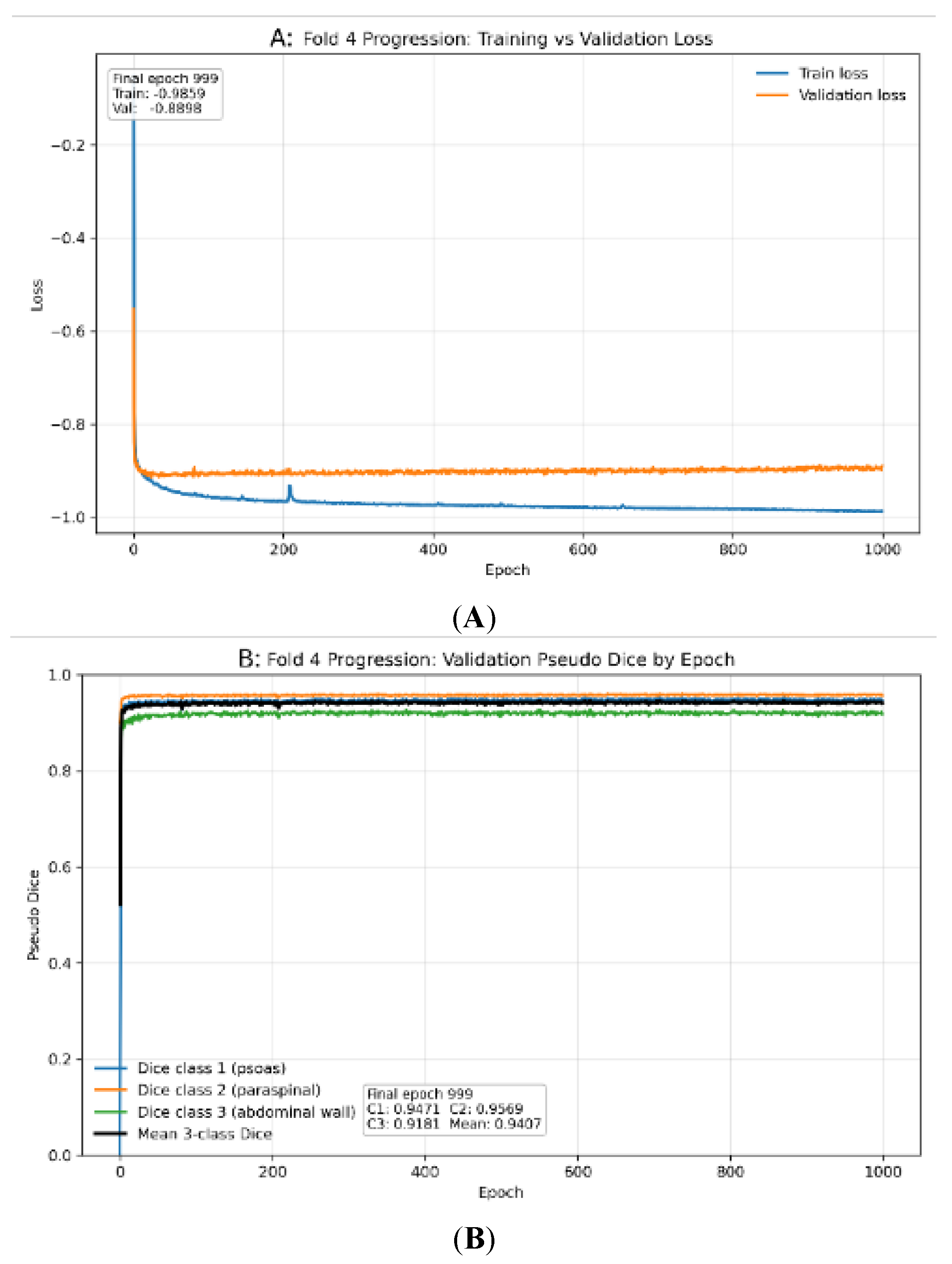
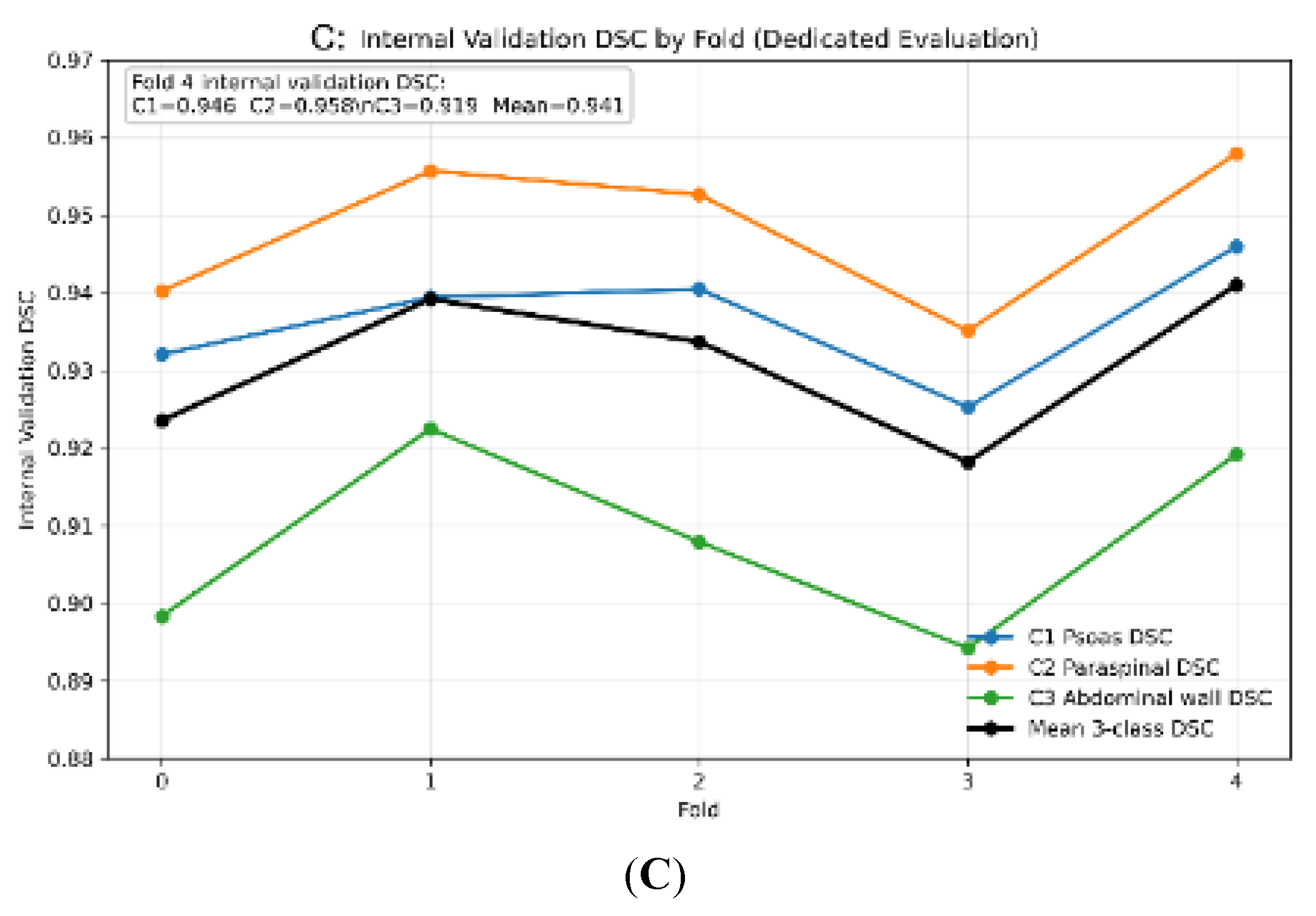
Figure 2.
The box-and-whisker plot illustrates the segmentation accuracy of the 5-fold ensemble 2D nnU-Net across 50 consecutive clinical cases. Horizontal lines denote the median Dice Similarity Coefficient (DSC), boxes represent the interquartile range (IQR), and whiskers extend to 1.5 times the IQR. The high median performance across all three muscle classes establishes the model’s generalizability to high-acuity, multi-vendor data.
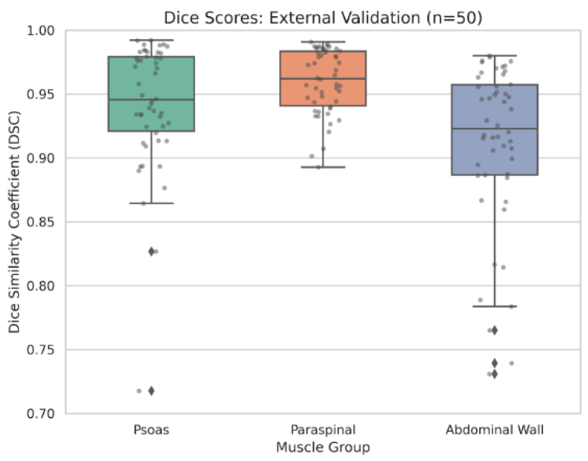
Figure 3.
The scatter plot with linear regression (solid line) shows the correlation between total cross-sectional area (cm²) of the abdominal muscle, quantified by the 5-fold ensemble 2D nnU-Net, and the manual reference standard. The high Pearson correlation coefficient (r = 0.955) confirms the clinical interchangeability of the automated volumetric muscle assessment pipeline.
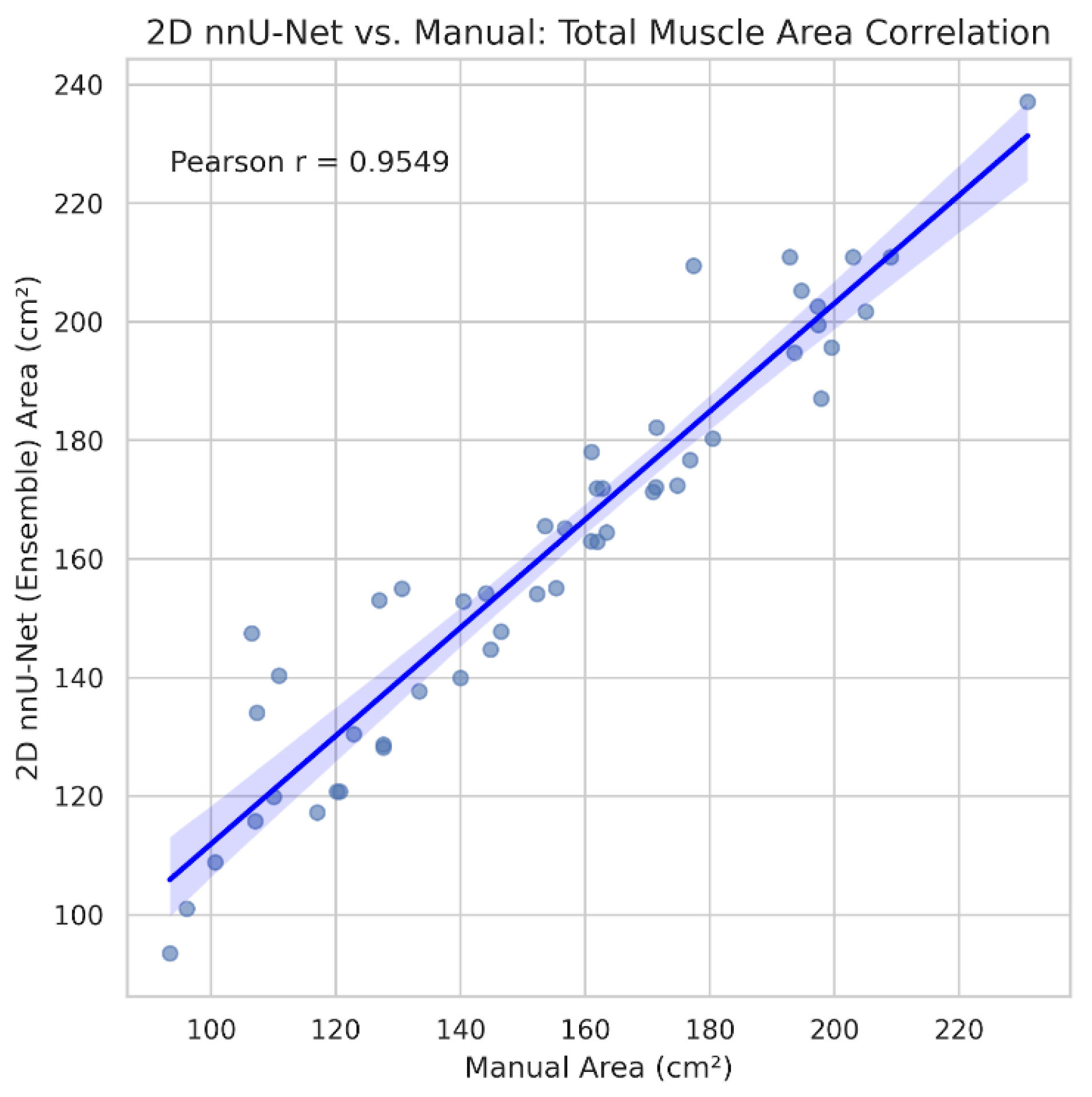
Figure 4.
The Bland-Altman plot assesses the measurement bias between the automated pipeline (5-fold ensemble 2D nnU-Net) and manual segmentation. The black dashed horizontal line indicates the mean bias (+7.17 cm²), while dashed red lines represent the 95% limits of agreement. The marginal positive bias reflects the automated model’s systematic inclusion of thin fascial planes at the muscle-peritoneum interface.
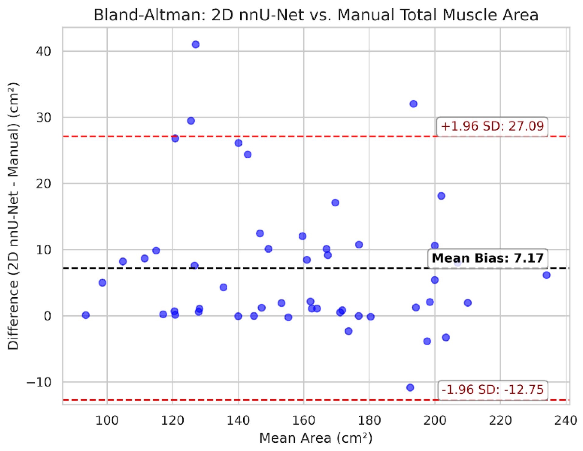
Figure 5.
The scatter plot illustrates the high correlation (r = 0.968) between the 5-fold ensemble 2D nnU-Net and manual reference for mean muscle density (HU). Accurate automated HU extraction is critical for the downstream evaluation of myosteatosis.
Figure 5.
The scatter plot illustrates the high correlation (r = 0.968) between the 5-fold ensemble 2D nnU-Net and manual reference for mean muscle density (HU). Accurate automated HU extraction is critical for the downstream evaluation of myosteatosis.
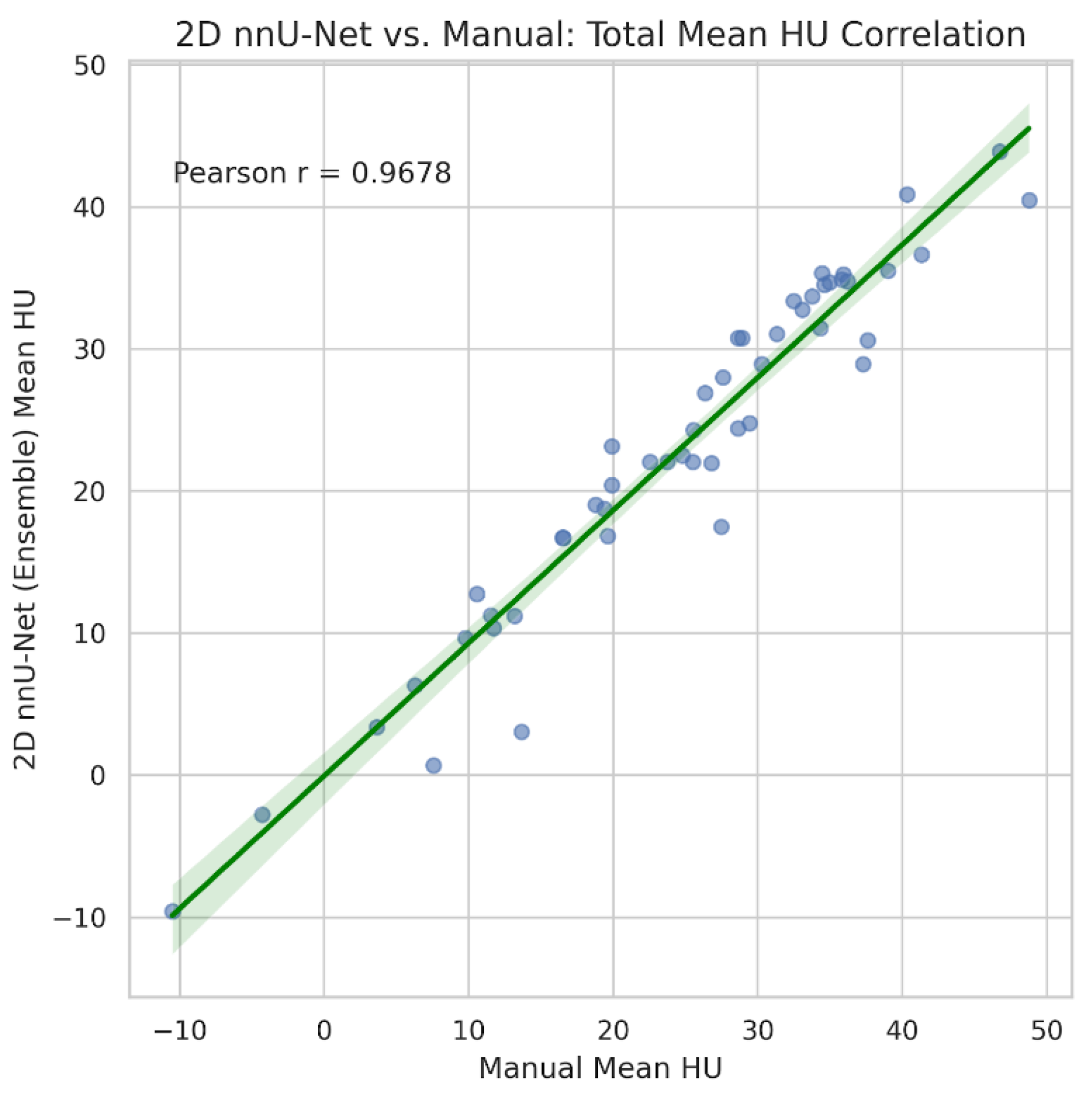
Figure 6.
The scatter plot assesses the reproducibility of the manual segmentations (n=30). The high Pearson correlation coefficient (r = 0.995) validates the stability of the reference standard utilized for external model evaluation.
Figure 6.
The scatter plot assesses the reproducibility of the manual segmentations (n=30). The high Pearson correlation coefficient (r = 0.995) validates the stability of the reference standard utilized for external model evaluation.
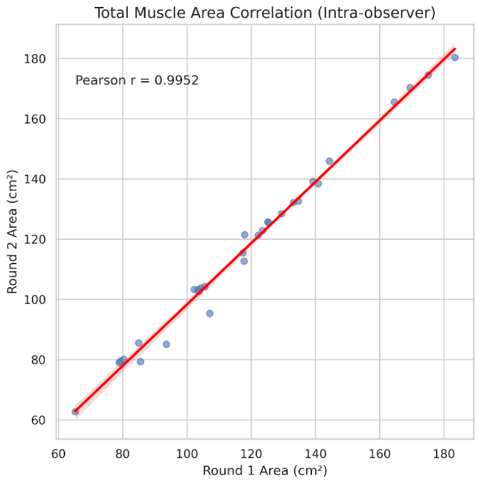
Figure 7.
Bland-Altman plot for intra-observer total muscle area. The minimal mean bias (-1.31 cm²) and narrow limits of agreement indicate consistent performance by the human reader following a 14-day washout period, establishing a stringent performance ceiling.
Figure 7.
Bland-Altman plot for intra-observer total muscle area. The minimal mean bias (-1.31 cm²) and narrow limits of agreement indicate consistent performance by the human reader following a 14-day washout period, establishing a stringent performance ceiling.
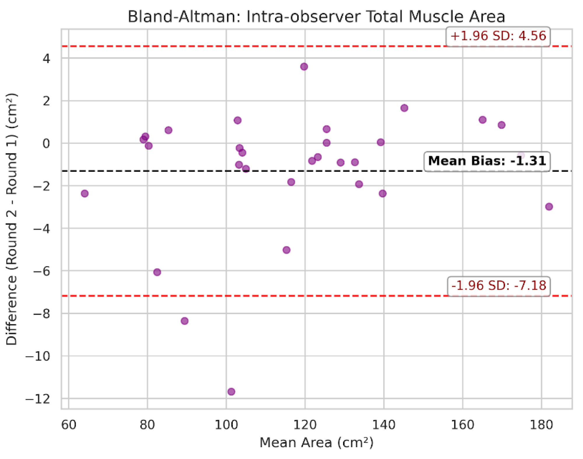
Figure 8.
Upper-bound segmentation performance. Representative axial L3 CT slice from the external validation cohort demonstrating optimal model performance in standard cross-sectional anatomy. Panels display the unannotated axial CT (A), manual reference standard (B), and automated ensemble prediction (C). Target classes are color-coded (red = psoas, green = paraspinal, blue = abdominal wall). The overall mean DSC was 0.988. High spatial overlap was achieved across all individual classes: psoas (DSC: 0.992), paraspinal (DSC: 0.991), and abdominal wall (DSC: 0.980). The automated prediction closely aligns with the manual reference standard, without erroneously including adjacent tissues.
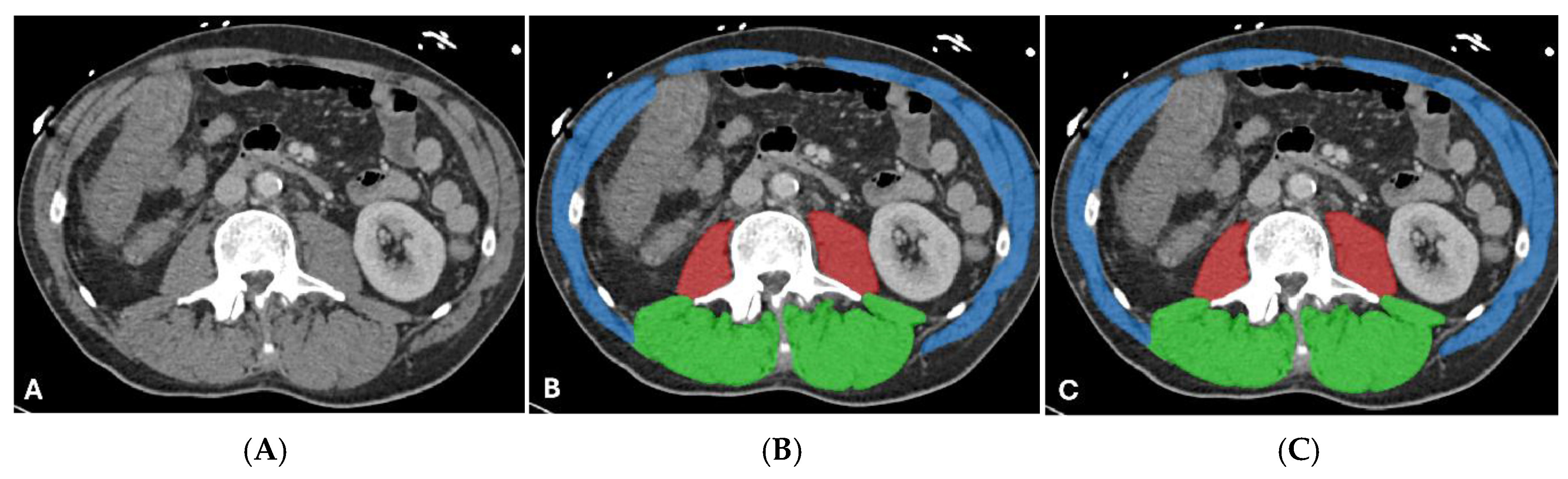
Figure 9.
Lower-bound segmentation performance in complex anatomy. Representative axial L3 CT slice from the external validation cohort demonstrating limited model performance in a patient with ascites. Panels display the unannotated non-contrast CT (A), manual reference standard (B), and automated ensemble prediction (C). Target classes are color-coded (red = psoas, green = paraspinal, blue = abdominal wall). The overall mean DSC was 0.822. Psoas segmentation (DSC: 0.718) was limited by the inclusion of the isodense left kidney (double arrows) on unenhanced imaging. Abdominal wall segmentation (DSC: 0.817) included portions of the peritoneum adjacent to the atrophic rectus abdominis (single arrow). The paraspinal muscle group maintained a higher spatial overlap (DSC: 0.933).
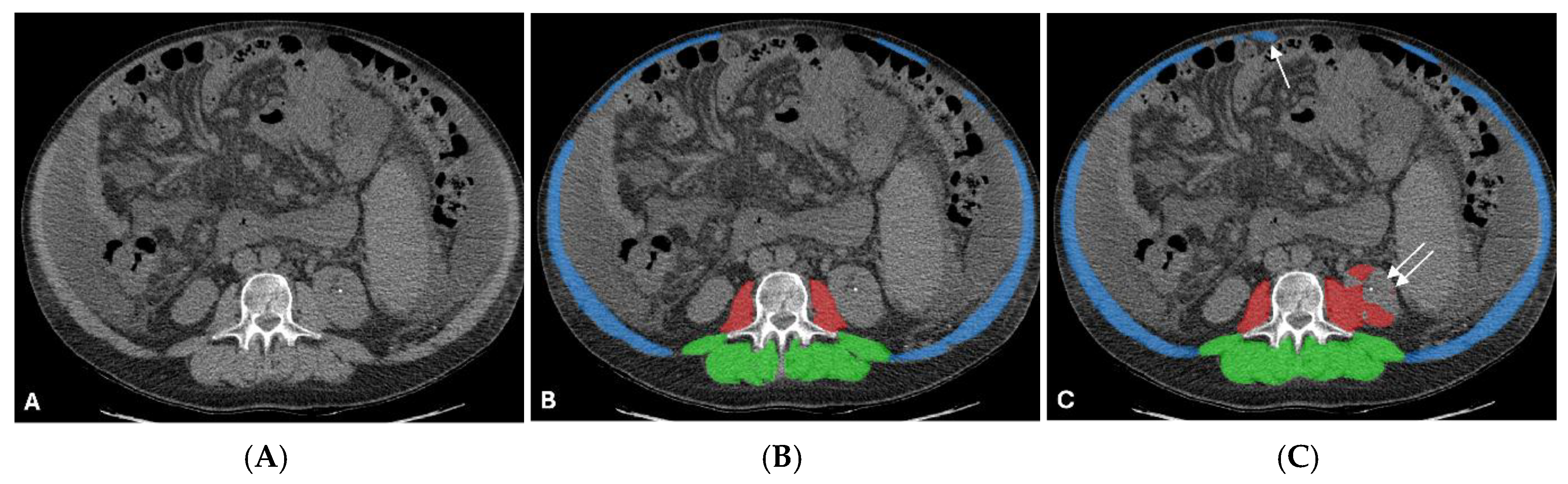
Figure 10.
Algorithmic misclassification associated with subcutaneous edema. Representative axial L3 CT slice from the internal training dataset demonstrating localized boundary failures in a patient with altered soft tissue density. Panels display the unannotated CT (A), manual reference standard (B), and automated prediction (C). Target classes are color-coded (red = psoas, green = paraspinal, blue = abdominal wall). Spatial overlap was reduced across all classes, psoas (DSC: 0.655), paraspinal (DSC: 0.648), and abdominal wall (DSC: 0.744). The psoas prediction undersegments the left psoas (single red arrow) and bridges into the left paraspinal compartment (single long white arrow). The paraspinal boundary extends into the posterior subcutaneous edema (double short white arrows). The abdominal wall boundary undersegments the bilateral oblique muscles (*) and includes a focal region of left posterior edema (double short red arrows) and the right posterior skin (white arrow).
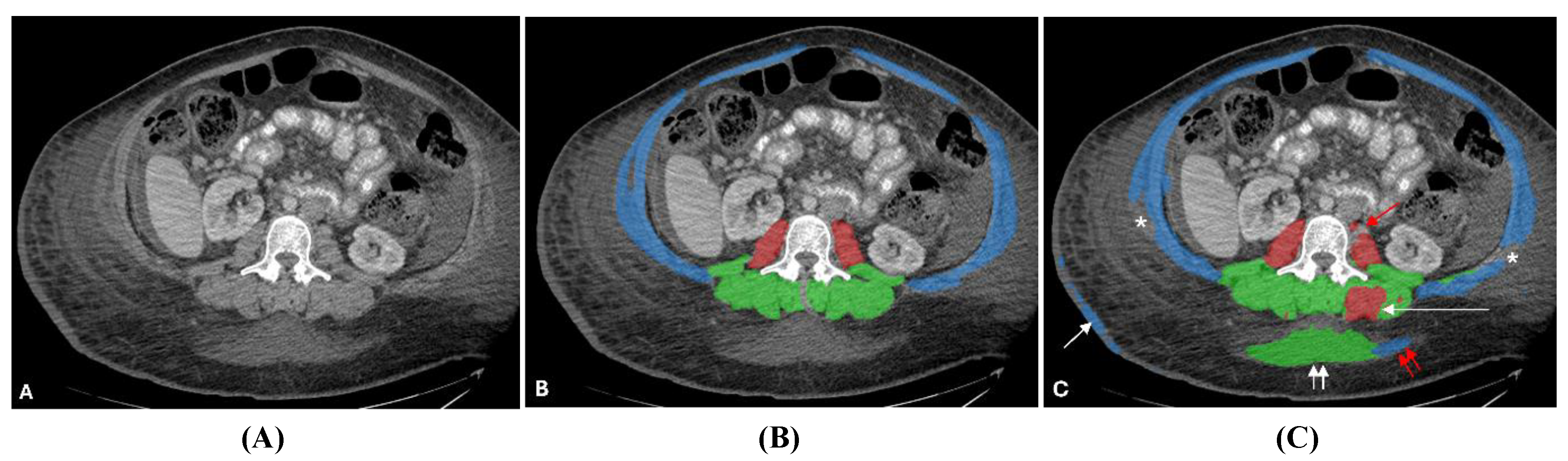

Table 1.
Demographics and clinical characteristics of the external validation cohort.
| Characteristic | Value |
|---|---|
| Total Cases (n) | 50 |
| Age (years) | 63 ± 15 |
| Sex (Male : Female) | 18 : 32 |
| Primary Clinical Indications (n, %) | |
| Liver cirrhosis | 11 (22%) |
| Routine evaluation for TIPS | 10 (20%) |
| Refractory ascites | 9 (18%) |
| Hepatocellular carcinoma | 8 (16%) |
| Portosystemic shunt | 6 (12%) |
| PV thrombosis evaluation | 5 (10%) |
| Hepatic hydrothorax | 3 (6%) |
| Axial CT Findings at L3 | |
| Ascites | 44 (88%) |
| Subcutaneous edema | 3 (6%) |
| Liver masses | 1 (2%) |
| No ascites | 6 (12%) |
Table 2.
Internal 5-Fold Cross-Validation Segmentation Performance.
| Fold | Psoas | Paraspinal | Abdominal wall | Mean DSC |
|---|---|---|---|---|
| 0 | 0.932 | 0.940 | 0.898 | 0.924 |
| 1 | 0.939 | 0.956 | 0.923 | 0.939 |
| 2 | 0.941 | 0.952 | 0.908 | 0.934 |
| 3 | 0.925 | 0.935 | 0.894 | 0.918 |
| 4 | 0.946 | 0.958 | 0.919 | 0.941 |
| Mean | 0.937 | 0.948 | 0.908 | 0.931 ± 0.010 |
DSC = Dice similarity coefficient.
Table 3.
External validation: single-fold vs. 5-fold ensemble architecture:.
| Metric | Single fold (Fold 4) | 5-fold ensemble | P-value |
|---|---|---|---|
| Overall mean DSC | 0.937 | 0.937 | 0.736 |
| Psoas DSC | 0.939 | 0.941 | 0.448 |
| Paraspinal DSC | 0.960 | 0.960 | 0.810 |
| Abdominal wall DSC | 0.912 | 0.911 | 0.858 |
| Minimum observed DSC | 0.720 | 0.822 | — |
Table 4.
Clinical measurement agreement: 2D nnU-Net vs. manual reference:.
| Metric | Pearson r | MAE | Mean bias (nnU-Net - manual) |
|---|---|---|---|
| Total muscle area (cm²) | 0.955 | 8.00 | +7.17 |
| Total mean attenuation (HU) | 0.968 | 2.33 | -1.67 |
Table 5.
Intra-observer reliability for the manual reference standard.
| Metric | Pearson r | MAE | Mean bias (round 2 - round 1) |
|---|---|---|---|
| Total muscle area (cm²) | 0.995 | 1.98 | -1.31 |
| Total mean attenuation (HU) | 0.995 | 0.74 | +0.56 |
Disclaimer/Publisher’s Note: The statements, opinions and data contained in all publications are solely those of the individual author(s) and contributor(s) and not of MDPI and/or the editor(s). MDPI and/or the editor(s) disclaim responsibility for any injury to people or property resulting from any ideas, methods, instructions or products referred to in the content. |
© 2026 by the authors. Licensee MDPI, Basel, Switzerland. This article is an open access article distributed under the terms and conditions of the Creative Commons Attribution (CC BY) license (http://creativecommons.org/licenses/by/4.0/).
Copyright: This open access article is published under a Creative Commons CC BY 4.0 license, which permit the free download, distribution, and reuse, provided that the author and preprint are cited in any reuse.


