Submitted:
18 February 2026
Posted:
26 February 2026
You are already at the latest version
Abstract
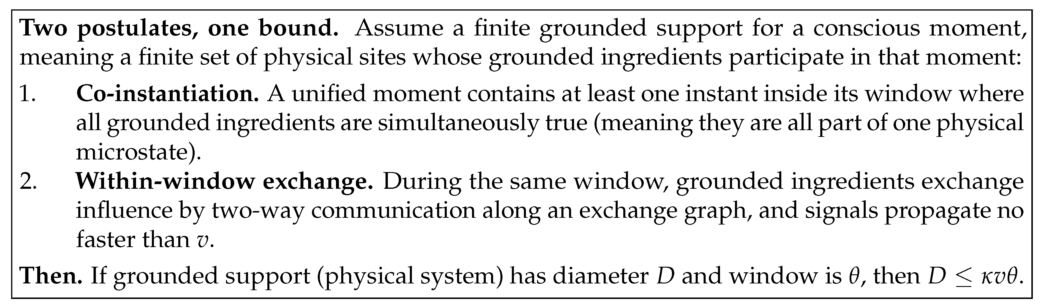
A conscious moment feels instantaneous, yet its ingredients are spread out in space, so signals take time to travel and integration must occur within a window of duration θ. In Stack Theory, Occurrence means each ingredient is true at least once within the window, while CoInstantiation means all are true together at some time. The Temporal Gap is Occurrence without CoInstantiation. Here, I show that if unity requires CoInstantiation and ingredients must exchange causal influence within window under a signal speed ceiling v, then the system diameter D satisfies D ≤ κvθ, with κ = 1 for hub exchange and κ = 1/2 for all-to-all exchange. A minimal message passing model shows fragmentation at these thresholds. Primate corpus callosum data imply size lower bounds on θ. This may rule out co-instantiated consciousness for liquid brains like ant colonies, AI on contemporary hardware, and it implies size constraints for proposed human–AI hybrids.
Keywords:
consciousness
; cognition
; stack theory
; unity
; conscious binding
Introduction
A conscious moment feels like a unified scene. An instant of time. Yet brains are spatially extended and coordination takes time. This raises the question of how an experienced “instant” works in relation to the objective progression of physical events in time.
To deal with this, many accounts of consciousness posit a temporal integration window of duration . Within this window the system is allowed to gather and bind a set of ingredient facts (sense, feeling, thought etc to which one has reportable conscious access [1]). An ingredient is a grounded physical fact, meaning a property of the underlying microstate rather than a purely internal label. Microstate here means the full physical state at the resolution where the ingredients live. At the neuronal scale, for example, it could mean the full pattern of spikes, membrane potentials, and synaptic states. This windowing idea is widespread. For example it appears in global workspace accounts [2,3], recurrent processing theories [4], dynamical synchrony [5,6,7], integrated information [8] and stack theoretic proposals [9,10,11,12]. In Stack Theory, meaning is ontological. The meaning of a statement is its truth set, which is the set of microstates that satisfy it. It also appears in classic philosophical discussions of subjective timing [13]. Empirically, psychophysics supports integration on the order of tens to hundreds of milliseconds, with task-dependent structure [14,15,16,17].
A window may be necessary, but it is not sufficient for literal co-presence [12]. Each ingredient can occur somewhere inside the window even when there is no instant at which they are all true together in the underlying physical state. I call that mismatch the Temporal Gap. In this paper Occurrence means every ingredient becomes true at least once during the window. CoInstantiation means there exists an instant during the same window when all ingredients are true together. Occurrence is like ticking each checkbox at least once somewhere in the window. CoInstantiation is like there being a moment when every checkbox is ticked at once. In what follows, I treat CoInstantiation as the requirement for a unified moment in the strong sense studied here. Occurrence is the weaker alternative. It only requires that each ingredient appears at least once somewhere in the window. Formal definitions appear in Definitions 2 and 3.
This paper does three things.
- 1.
- It extends Stack Theory to time semantics of Occurrence versus CoInstantiation (extending this workshop paper [12]).
- 2.
- It adds a minimal within-window causal exchange postulate and derives a spacetime diameter bound for one unified moment.
- 3.
- It builds a falsification pipeline, validates it with stress tests, and anchors the bound using a reanalysis with no new data collection of published primate corpus callosum microstructure.
Everything that follows is conditional. If the CoInstantiation requirement is wrong, or if within-window exchange is not required, the diameter bound does not apply.
Notation preview.
A candidate moment is a time window . D is the diameter of the grounded support, meaning the largest distance across the physical sites that carry the grounded ingredients. v is an upper bound on causal propagation speed in the relevant substrate. is an architecture factor determined by which sites must exchange messages within one window.
Supplementary Note 0 in the SI is a glossary and figure reading guide for the technical terms and plots. If you are coming from another discipline, start there.
Temporal integration windows are not new. The novelty here is turning the CoInstantiation requirement plus a minimal within-window exchange requirement into a falsifiable spatial inequality with an explicit architecture factor. If a moment must be causally knitted together within its own window, then unity has a speed limit. That speed limit converts into a size limit. To put it provocatively, a conscious mind can only be so big for a given signal speed.
Figure 1.
To get a big unified moment, you pay for it using time, speed, or architecture.
Results
Windowing Is Weaker Than Simultaneity
I represent the content of a candidate moment using a Stack Theory abstraction layer [18]. An abstraction layer is built from an environment and a finite vocabulary . I define these objects next. The key modelling choice is extensional semantics. It treats each ingredient as a physical constraint and it treats meaning as the set of microstates that satisfy that constraint.
Definition 1
(Environment, programs, statements, and truth sets). An environment is a nonempty set Φ of mutually exclusive microstates. For any set X, write for its power set, meaning the set of all subsets of X. A program is any set . Write for the set of all programs. A vocabulary is a finite set of programs that a system can implement. The induced embodied language is
Elements are called statements. The truth set of a statement is
Narrative interpretation.
A microstate is one fully specified physical configuration. A program is a yes or no property of microstates, represented by the set of microstates where it holds. In Stack Theory, the word program does not mean executable code. It means a physically implementable predicate. The notation means all subsets of . It is the set of all possible programs you could define. A vocabulary is the particular finite menu of programs this system can actually implement. A statement ℓ is a bundle of programs that can all be true together. Because the vocabulary is finite, every statement is automatically a finite bundle. Its truth set is the set of physical states where the whole bundle is true at once. In this paper an ingredient is one program . The vocabulary is finite because an embodied system has finite information capacity [19,20]. The Bekenstein bound is one concrete physics limit of this kind. It upper bounds how much information a finite region can store. You do not need to accept the Bekenstein bound in particular. Any finite physical memory implies a finite menu of physically distinguishable conditions at a chosen resolution. That is why treating vocabularies as finite is a reasonable modelling default. In Stack Theory, the pair plus its induced language is the abstraction layer used in this manuscript. Supplementary Note 2 restates the Stack Theory definitions used here.
Temporal binding introduces a window of duration . Let denote the underlying microstate at objective time . I call a program grounded when it is evaluated directly on in the base environment , rather than inside a separate internal label space [12].
Definition 2
(Occurrence and co-instantiation). Fix a statement and a time window . Ingredient-wise occurrence holds when each ingredient becomes true at least once somewhere inside the window.
Co-instantiation holds when there exists at least one instant inside the window at which all grounded ingredients are simultaneously true.
Definition 3
(Temporal Gap). Fix a statement and a time window . The Temporal Gap event is when every ingredient occurs somewhere inside the window, but there is no instant inside the window when they are all true together.
Narrative interpretation.
The symbol is just shorthand for the window . Occurrence says each ingredient shows up at least once somewhere inside the window. CoInstantiation says there is at least one instant when the ingredients overlap in the underlying physical state. CoInstantiation automatically implies Occurrence. If all ingredients are true together at one instant, then each ingredient occurs at that instant. Occurrence is therefore a weaker criterion than CoInstantiation. The Temporal Gap is the mismatch where Occurrence holds but CoInstantiation fails. It is illustrated in Figure 2.
This gap matters because if consciousness requires an instant at which the ingredients are all grounded together, then the theory needs a synchrony condition, not just a set of events that happen separately within a shared clock interval.
Diameter Bound
I add a within-window causal exchange postulate. If ingredients are jointly instantiated, then the sites that host those ingredients must be able to exchange causal influence within the same window.
Assumption A1
(Within-window causal exchange). Let be the physical substrate equipped with a metric ρ. Let be a finite grounded support for a moment, meaning a finite set of physical sites whose grounded ingredients participate in that moment. Define its diameter by
Assume there exists a connected undirected exchange graph . For every required edge there are causal travel times such that a round trip fits inside the window
Signals propagate no faster than v. Equivalently, each one-way travel time must satisfy and .
Narrative interpretation.
v is a speed limit (not to be confused with the embodied vocabulary symbol ). A metric is just a rule for distance that behaves like ordinary distance and obeys the triangle inequality. Triangle inequality means going from a to c directly is never longer than going from a to b to c. Connected means you can reach any site from any other site by hopping along required exchange edges. If the exchange graph is not connected, your candidate moment is already fragmented into components, so apply the bound component by component. Pick the physical sites that are supposed to contribute grounded ingredients to the moment. A site can be a neuron, a cortical column, a brain region, or any other spatial unit that makes sense for the modelling scale. Draw an edge between two sites if your theory says those two sites must be able to influence each other within one window. The travel times and are the message times in each direction. The inequality says there is time for a signal to go out and for an acknowledgement to come back within the same moment. The speed bound v says these travel times cannot be arbitrarily small because no signal can outrun v. Together with the round trip budget, this implies that every required edge can span at most of physical distance.
Pick the distance rule and the speed bound v as a matched pair. If you measure as straight line distance, then v should be an effective speed that already includes wiring detours. If you measure as path length along fibres or wires, then v can be a more direct conduction speed along that path.
The exchange graph specifies who has to talk to whom within one subjective moment. The round trip condition is the minimal way of cashing out the idea that a moment is causally stitched together rather than merely co-timed.
In the limits the architecture can be a hub, an all-to-all mesh, or a general graph. Each architecture determines a geometric constant that converts time into diameter. The formal graph definition of and the proof are in Supplementary Note 3.
Theorem 1
(Spacetime diameter bound). Under Assumption A1, the grounded support diameter satisfies
For hub exchange, meaning a star graph, . For all-to-all exchange, meaning a complete graph, . In general, let be the length in edges of a shortest path between u and in G. Define the hop diameter
Then .
Narrative interpretation.
A star graph is a hub and spokes. A complete graph connects every pair directly. The hop distance counts how many required handoffs a message must make to get from u to . The hop diameter is the worst case hop count across the whole support. The constant is therefore a pure architecture factor. Each hop can span at most of physical distance because a round trip must fit inside the window. So the bound says the diameter is at most hops worth of distance, which is exactly .
Units reminder.
D is a distance. v is distance per time. is time. So is a distance and is dimensionless.
Worked example.
Suppose and . Then . Under hub exchange, meaning , the bound gives . Under all-to-all exchange, meaning , the bound gives . These are order of magnitude numbers. The point is that a time budget becomes a size budget.
In other words, if the window is too short for causal exchange across the support, there is no way to knit the ingredients into one co-instantiated state. See Figure 3 for a basic illustration.
Fragmentation Transition
Theorem 1 is a worst case bound. To see whether the same geometry shows up in a concrete mechanism, I build a minimal message-passing model.
There are N sites arranged on a circle of diameter D. A moment is a window of duration . Signals propagate at speed at most v, so a one-way message over distance d has baseline travel time . On top of this baseline each directed message receives an independent exponential jitter term with mean . Exponential here means most messages are close to their baseline travel time but a few run very late. It is a simple way to model rare but consequential delays. Here j is dimensionless and can be read as the expected fraction of the window lost to random delays.
I evaluate two exchange graphs. Hub exchange means a star graph. All-to-all exchange means a complete graph. The model declares the moment integrated only if every required edge completes a two-way exchange within the same window. This yields an exact success probability. Success probability is the chance, over the random jitter, that the window meets this integration requirement. Supplementary Note 4 gives the derivation.
To present results compactly, define the dimensionless size ratio
This ratio is the fraction of the window needed to traverse the diameter at speed v.
Narrative interpretation.
x is a unitless tightness score. It compares the best case time to cross the support once, , to the time you have, . Small x means plenty of slack. Large x means you are spending most of the window just moving signals around. A run of the mechanistic model counts as a success only if every required two-way exchange finishes before the window ends. Figure 4a plots this success probability as a function of x. The curves stay close to 1 for a while and then drop rapidly toward 0. That rapid drop is what I mean by collapse here. It is the point where the window becomes too tight for within-window exchange. Hub exchange drops near . All-to-all exchange drops near .
Figure 4b is a robustness sweep. A sweep means rerunning the same model many times while changing input parameters. Here I vary two nuisance parameters, the number of sites N and the jitter level j. j is the mean random extra delay per message written as a fraction of the window. For each setting I summarise the transition by , the value of x where the success probability is . Across and I obtain
The key point is that stays close to the theoretical thresholds. This suggests the transition is not a fragile artifact of one particular choice of N and j.
Primate Scaling Anchor
How does this bound manifest in the real world? To glean some insight into this, I anchor it using an existing primate dataset that is already published and does not require new experiments.
The corpus callosum is the major fibre tract connecting the two cerebral hemispheres. Any moment that requires causal exchange between hemispheres cannot complete faster than the relevant callosal conduction time.
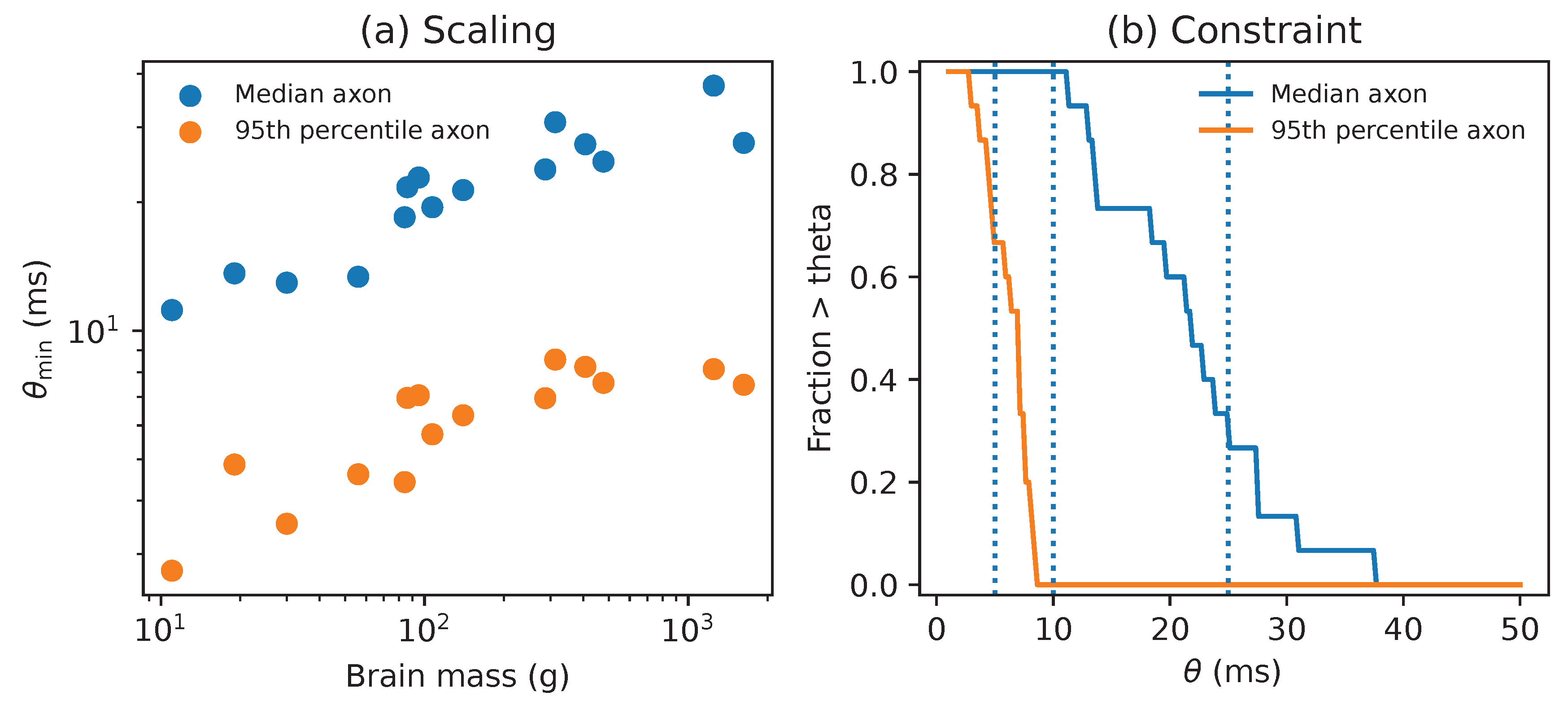
Phillips et al measured callosal axon diameter distributions across primates and reported implied one-way interhemispheric conduction times for two fibre proxies [21,22]. The corrected Table 1 contains individual primates across 14 primate species. The scaling fits below are descriptive. They are not a phylogeny-aware comparative analysis that corrects for shared ancestry. One proxy uses the median axon diameter. The other uses the 95th percentile axon diameter as a fast fibre proxy. I use these implied conduction times as reported in the corrected Table 1, rather than recomputing them. These one-way delays are hard floors on any integration window that needs information to cross between hemispheres. Under the stronger two-way exchange postulate used elsewhere in this paper, a round trip constraint would be roughly twice these values. The scaling pattern is unchanged because the factor is constant. This does not claim that callosal delay alone determines consciousness. It only supplies a physically grounded timescale that any bilateral moment must at least accommodate. It is an illustration using real world data. Interhemispheric conduction delay has long been proposed as a constraint on integration and hemispheric specialisation, and it scales with brain size [23,24,25]. Figure 5a plots the implied lower bound versus brain mass. On a log-log fit, the median axon proxy scales with exponent with bootstrap interval and . A bootstrap interval is an uncertainty interval computed by resampling the data. is the usual fraction of variance explained by the fit. Supplementary Note 6 describes the regression and bootstrap procedure used to compute these values. It also explains how to read the primate plots. The fast axon proxy scales with exponent with interval and . Across the sample, brain mass spans a factor 148 while spans factors and for median and fast proxies.
Figure 5b converts the same data into a direct constraint. For any candidate window , it reports the fraction of individuals whose reported conduction time exceeds . For example, of median proxy times exceed 25 ms, while of fast proxy times exceed 5 ms.
Falsification and Stress Tests
Claims like are only scientifically useful if they can be falsified. Given data, the natural falsification target is the margin
Here is a diameter estimate for the candidate support, is the candidate window duration, and is an estimate of the fastest relevant causal propagation speed. A violation corresponds to .
Testing protocol.
To test this bound:
- 1.
- Pick a candidate unity marker and a window duration .
- 2.
- For each window, estimate the support diameter and collect fast-propagation samples to estimate .
- 3.
- Compute the margin .
- 4.
- If windows overlap heavily, thin them by keeping every kth window.
- 5.
- Test whether the mean margin is greater than zero using a one sided t test.
The fiddly part is . If you underestimate the true speed ceiling, you can manufacture violations. To stay conservative, I treat v as a sampled quantity and estimate using a high quantile, specifically the 95th percentile of the within-window samples. The 95th percentile is the value below which of the samples fall. Call this the q95 rule. q95 ignores the slow bulk and asks how fast the system can plausibly go.
I then test whether the mean margin across windows is positive using a one sided t test. This asks whether the average violation is reliably above zero, given sampling noise. Windows can be statistically dependent. To avoid overstating certainty, I control dependence by thinning. Thinning means keeping only every kth window so that the remaining windows are closer to independent. For example, if you slide a 50 ms window forward in 1 ms steps, then adjacent windows share almost all of their data. Keeping every 50th window removes that overlap. Thinning pretty much means making the overlap smaller. Supplementary Note 5 gives the full protocol. It also explains how to read each stress test plot. I validate the full pipeline using Monte Carlo based stress tests. I simulate windowed data where the true ratio is known, run the same falsification procedure, and measure false refutations and power. Power here means the probability of detecting a true violation. The stress tests support three takeaways.
- 1.
- The false refutation rate is controlled at or below the nominal level when v is conservatively estimated. Under the default q95 rule used here I observe no false refutations at ratio 1.00 in 2500 replications.
- 2.
- Power rises rapidly once the true ratio exceeds one. In these Monte Carlo tests I set as a units choice, so the x axis should be read as in general. With the conservative default quantile estimator used here and windows, the rise begins once the true ratio exceeds one by only a few percent.
- 3.
- Naive estimators that underestimate the relevant speed bound, especially low end choices like taking the minimum within-window sample, can manufacture violations and inflate false refutation dramatically.
All simulation code and source data are included.
Discussion
The inequality is a conditional claim about what a physically unified moment requires. It follows from two modelling commitments. The first commitment is the CoInstantiation requirement [12]. Unity requires not just that ingredients occur somewhere in a window, but that there exists an instant of objective time when the grounded ingredients are jointly true. This rules out the Temporal Gap. Stack Theory formalises this by making the joint truth condition membership in a joint truth set [12]. The second commitment is within-window causal exchange. If the ingredients are supposed to be one moment rather than a list, then they must be able to constrain each other by two-way communication within the same window. This turns a time budget into a spatial budget. If either commitment is false for the relevant notion of consciousness, then the bound does not apply as intended.
The mechanistic model shows that even a toy integration mechanism exhibits a sharp fragmentation transition near the theoretical thresholds. The primate reanalysis is a sanity check on scale. Callosal conduction time is one concrete example of latency that any bilateral moment must at least accommodate. The lower bound scales with brain size, consistent with the idea that larger brains either integrate more slowly, integrate more locally, or change architecture in a way that reduces .
Implications for Populations and Human-AI Hybrids
Hybrid cognition comes in progressive categories [26]. At one extreme, an AI is a prosthesis. It extends human agency but it does not participate as a grounded ingredient in the human moment. It fails when the system becomes too much for a human to directly control. Further along, humans, AIs and prosthetic human-AI hybrids can all be distinct agents that coordinate across time. This yields a cooperative hybrid, which fails when the goals of the AI and humans involved drift out of alignment [18]. Finally there can be integrated hybrids, where human and AI contributions are meant to participate in one co-instantiated moment, extending the conscious agency of a human further into a system of AIs. An integrated hybrid can facilitate larger prosthetic and co-operative hybrids, because human agency and alignment can extend further [26].
The spacetime bound constrains this last, strongest notion of integration. If the hybrid must co-instantiate grounded ingredients and complete within-window causal exchange, then the full hybrid support must fit inside the same latency budget. If any critical part of the control loop sits behind a high latency channel, the system cannot form one unified moment at that scale. What you get instead is two unified systems taking turns across moments, not one enlarged mind.
In this sense, integrated hybrids have an integration radius. Beyond that radius you do not get a bigger mind. You get a bigger committee.
This connects to the liquid brain versus solid brain distinction [27]. Solid brains have persistent high bandwidth wiring that can support tight within-window exchange across many sites. Liquid brains, such as ant colonies, compute through movement and have no persistent structure. They can solve problems through slow interactions between agents, but they do not have the bandwidth to support co-instantiated unity at the colony scale. On the present definition, they are not conscious in the strong co-instantiated sense. Finally, traditional computer architectures do not facilitate the sort of two way causal exchange or temporal co-instantiation I’ve talked about. This suggests contemporary computers cannot host consciousness.
Predictions and Falsifiers
Each falsifier targets a different modelling commitment.
- 1.
- Temporal Gap falsifier. Take any high time resolution recording where you can define a set of grounded ingredients ℓ and a candidate unity marker over windows of duration . A unity marker is any measurable variable that is supposed to indicate that one unified moment occurred, such as a phase synchrony measure or a behavioural report. For each window , compute and for the same ℓ. Then focus on windows where holds but fails. If the unity marker still behaves as if a single moment occurred in those windows, then the CoInstantiation requirement is wrong for that marker.
- 2.
- Latency budget violation. Pick any substrate where you can estimate a support diameter and a propagation ceiling for the same candidate unity marker. Write for a conservative lower bound on diameter, and write and for conservative upper bounds on speed and window duration. Compute the conservative margin . If is significantly positive across windows under the protocol in Supplementary Note 5, then either the within-window exchange postulate is false or the marker is not a unified moment.
- 3.
- Architecture factor shift. Hold the same nodes, the same geometry, and the same window definition. Change only the exchange graph. For engineered systems this means swapping between hub exchange, all-to-all exchange, and a chosen sparse graph. For the same measured v and , the largest diameter that still supports integration should scale in direct proportion to . If the transition does not move when moves, then the architecture factor model is wrong.
These are just sense checks on timestamps, distances, and who must talk to whom. A unified moment is the set of sites that can mutually exchange causal influence within a window of duration . Its spatial diameter cannot exceed . If you want a bigger subjective moment, you must either have more time for integration (somehow), propagate faster, or change the exchange architecture.
Methods
Stack Theory Objects and Temporal Lift
Definitions 1 and 2 give the formal objects used in the Results. I repeat the core pieces here for convenience.
An environment is a nonempty set of mutually exclusive microstates. A program is a set . A finite vocabulary is the set of programs a system can implement. The induced embodied language is
For , the truth set is , with .
To lift truth to time, let be the microstate trajectory. Occurrence, CoInstantiation, and the related synchrony conditions are defined in Definitions 2 and 3. Grounded means that the programs are evaluated directly on in the base environment.
Architecture Factor and Proof Idea
Supplementary Note 3 defines where is the hop diameter of an exchange graph G on the grounded support. In other words, counts the worst case number of message handoffs needed to connect the two most separated sites, given the required exchange edges.
Theorem 1 follows from one inequality. Assume each edge can complete a round trip within the window so . Then at least one direction has travel time at most . With propagation speed bounded by v this implies the metric distance between u and w is at most .
Any pair of sites is connected by a path of at most hops. The triangle inequality says the direct distance between two sites is at most the sum of distances along any path between them. So their separation is at most .
Mechanistic Integration Model
The mechanistic model places N contributor sites uniformly on a circle of diameter D. For all-to-all exchange I require a completed round trip for every unordered pair of sites, using the Euclidean chord distance on the circle. Chord distance is the straight line distance between two points on the circle. For hub exchange I model a central mediator at the circle centre, so each contributor must complete a round trip via the hub.
A directed message time is , where d is the one-way Euclidean distance and is exponential jitter with mean . A round trip time is therefore . Under the independence assumptions, overall success probability factorises over required exchanges.
Because is the sum of two independent exponential random variables, it has a Gamma distribution. I therefore evaluate success probability exactly using the closed form Gamma cumulative distribution function. In other words, this is just the probability that the random delay stays below the remaining time budget.
Primate Literature Extraction
The primate dataset is extracted from Phillips et al Table 1 [21] plus the published correction [22]. The corrected Table 1 contains individuals across 14 species. I include the extracted values in ttgs_phillips2015_table1.csv. I treat the reported interhemispheric conduction times as proxies for moments requiring bilateral exchange.
Monte Carlo Stress Tests
I simulate a measurement pipeline where D, , and v are observed with noise. For each simulated run I form the margin across windows and test whether its mean is positive with a one sided t test. In other words, this asks whether the average margin is reliably above zero given sampling noise.
I treat v as a sampled quantity and compare estimators. I also simulate dependence across windows with an AR(1) model. AR(1) means a first order autoregressive process, where each window is correlated with the previous one. I show that thinning controls false refutations. Thinning means keeping only every kth window so that the remaining windows are closer to independent. For example, if you slide a 50 ms window forward in 1 ms steps, then adjacent windows share almost all of their data. Keeping every 50th window removes that overlap.
Supplementary Materials
The following supporting information can be downloaded at the website of this paper posted on Preprints.org.
Author Contributions
The author conceived the study, developed the theory, performed the analyses, and wrote the manuscript.
Data Availability Statement
All simulation outputs and source data tables are generated by ttgs_simulation.py and written into the ttgs_source_data directory. The primate dataset extracted from published literature is included as ttgs_phillips2015_table1.csv. Source data are provided with this paper.
Code Availability
All code required to reproduce the figures and tables is provided in ttgs_simulation.py. Running python ttgs_simulation.py regenerates every figure, LaTeX macro file, and source data CSV used by this manuscript. The same run writes ttgs_provenance.json, a machine readable record of every literature derived numeric input and its stable identifier. A one page reproducibility and data provenance checklist is provided as TTGS80_ReproChecklist.pdf.
Acknowledgments
The author thanks colleagues and early readers for feedback that improved the manuscript.
Conflicts of Interest
The author declares no competing interests.
References
- Block, N. On a confusion about a function of consciousness. Behavioral and Brain Sciences 1995, 18, 227–247. [Google Scholar] [CrossRef]
- Baars, B.J. A Cognitive Theory of Consciousness; Cambridge University Press: Cambridge, 1988. [Google Scholar]
- Dehaene, S.; Naccache, L. Towards a cognitive neuroscience of consciousness: basic evidence and a workspace framework. Cognition 2001, 79, 1–37. [Google Scholar] [CrossRef]
- Lamme, V. Towards a True Neural Stance On Consciousness. Trends in cognitive sciences 2006, 10, 494–501. [Google Scholar] [CrossRef] [PubMed]
- Varela, F.J.; Lachaux, J.P.; Rodriguez, E.; Martinerie, J. The brainweb: phase synchronization and large-scale integration. Nature Reviews Neuroscience 2001, 2, 229–239. [Google Scholar] [CrossRef] [PubMed]
- Singer, W.; Gray, C.M. Visual feature integration and the temporal correlation hypothesis. Annual Review of Neuroscience 1995, 18, 555–586. [Google Scholar] [CrossRef] [PubMed]
- Fries, P. A mechanism for cognitive dynamics: neuronal communication through neuronal coherence. Trends in Cognitive Sciences 2005, 9, 474–480. [Google Scholar] [CrossRef]
- Tononi, G. An information integration theory of consciousness. BMC Neuroscience 2004, 5, 42. [Google Scholar] [CrossRef]
- Bennett, M.T. Emergent Causality and the Foundation of Consciousness. In Proceedings of the 16th International Conference on Artificial General Intelligence Lecture Notes in Computer Science; Springer; OUCI metadata page, 2023; pp. 52–61. Available online: https://ouci.dntb.gov.ua/en/works/7BoXJMW4/.
- Bennett, M.T.; Welsh, S.; Ciaunica, A. Why Is Anything Conscious? Preprint 2024, arXiv:cs. [Google Scholar] [CrossRef]
- Bennett, M.T. How To Build Conscious Machines. PhD thesis, The Australian National University, 2025. [Google Scholar] [CrossRef]
- Bennett, M.T. A Mind Cannot Be Smeared Across Time. arXiv 2026, arXiv:cs. [Google Scholar] [CrossRef]
- Dennett, D.C.; Kinsbourne, M. Time and the observer: the where and when of consciousness in the brain. Behavioral and Brain Sciences 1992, 15, 183–201. [Google Scholar] [CrossRef]
- Eagleman, D.M.; Sejnowski, T.J. Motion integration and postdiction in visual awareness. Science 2000, 287, 2036–2038. [Google Scholar] [CrossRef] [PubMed]
- Pöppel, E. A hierarchical model of temporal perception. Trends in Cognitive Sciences 1997, 1, 56–61. [Google Scholar] [CrossRef] [PubMed]
- Vroomen, J.; Keetels, M. Perception of intersensory synchrony: a tutorial review. Attention, Perception, & Psychophysics 2010, 72, 871–884. [Google Scholar] [CrossRef] [PubMed]
- Wallace, M.T.; Stevenson, R.A. The construct of the multisensory temporal binding window and its dysregulation in developmental disabilities. Neuropsychologia 2014, 64, 105–123. [Google Scholar] [CrossRef]
- Bennett, M.T. Are Biological Systems More Intelligent Than Artificial Intelligence? Philosophical Transactions of the Royal Society B: Biological Sciences. Special issue on Hybrid agencies: crossing borders between biological and artificial worlds 2024, arXiv:cs. [Google Scholar] [CrossRef]
- Bekenstein, J.D. Universal upper bound on the entropy-to-energy ratio for bounded systems. Phys. Rev. D 1981, 23, 287–298. [Google Scholar] [CrossRef]
- Bennett, M.T. Is Complexity an Illusion? In Proceedings of the 17th International Conference on Artificial General Intelligence, 2024; Springer; Lecture Notes in Computer Science. [Google Scholar] [CrossRef]
- Phillips, K.A.; Stimpson, C.D.; Smaers, J.B.; Raghanti, M.A.; Jacobs, B.; Popratiloff, A.; Hof, P.R.; Sherwood, C.C. The corpus callosum in primates: processing speed of axons and the evolution of hemispheric asymmetry. Proceedings of the Royal Society B: Biological Sciences 2015, 282, 20151535. [Google Scholar] [CrossRef]
- Phillips, K.A.; Stimpson, C.D.; Smaers, J.B.; Raghanti, M.A.; Jacobs, B.; Popratiloff, A.; Hof, P.R.; Sherwood, C.C. Correction to The corpus callosum in primates: processing speed of axons and the evolution of hemispheric asymmetry. Proceedings of the Royal Society B: Biological Sciences 2015, 282, 20152620. [Google Scholar] [CrossRef]
- Ringo, J.L.; Doty, R.W.; Demeter, S.; Simard, P.Y. Time is of the essence: a conjecture that hemispheric specialization arises from interhemispheric conduction delay. Cerebral Cortex 1994, 4, 331–343. [Google Scholar] [CrossRef]
- Caminiti, R.; Ghaziri, H.; Galuske, R.A.W.; Hof, P.R.; Innocenti, G.M. Evolution amplified processing with temporally dispersed slow neuronal connectivity in primates. Proceedings of the National Academy of Sciences of the United States of America 2009, 106, 19551–19556. [Google Scholar] [CrossRef]
- Innocenti, G.M.; Vahlsing, I.; Caminiti, R. The functional characterization of callosal connections. Progress in Neurobiology 2022, 208, 102186. [Google Scholar] [CrossRef]
- Solé, R.; Seoane, L.F.; Pla-Mauri, J.; Bennett, M.T.; Hochberg, M.E.; Levin, M. Cognition spaces: natural, artificial, and hybrid. 2026, 2601.12837. [Google Scholar] [CrossRef]
- Solé, R.; Moses, M.; Forrest, S. Liquid brains, solid brains. Philosophical Transactions of the Royal Society B: Biological Sciences 2019, 374, 20190040. Available online: https://royalsocietypublishing.org/doi/pdf/10.1098/rstb.2019.0040. [CrossRef]
Figure 2.
Both occur in the window, but never at the same instant. This is the Temporal Gap. Occurrence can hold without co-instantiation.
Figure 2.
Both occur in the window, but never at the same instant. This is the Temporal Gap. Occurrence can hold without co-instantiation.
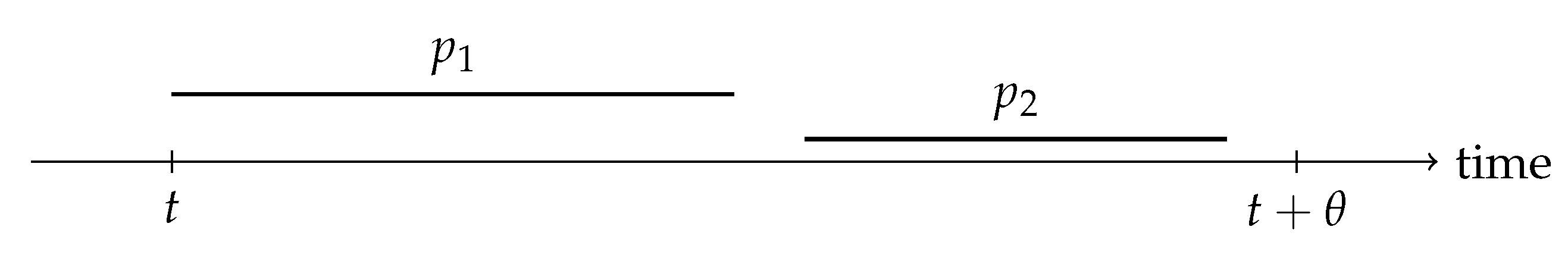
Figure 3.
Geometry underlying the bound. It is a worst case. In a star architecture, the farthest pair of contributors communicates in two hops via the hub, so each hop must fit inside half the window and the overall diameter budget is . In a complete architecture, the farthest pair must complete a round trip over distance D within the window, giving the tighter budget .
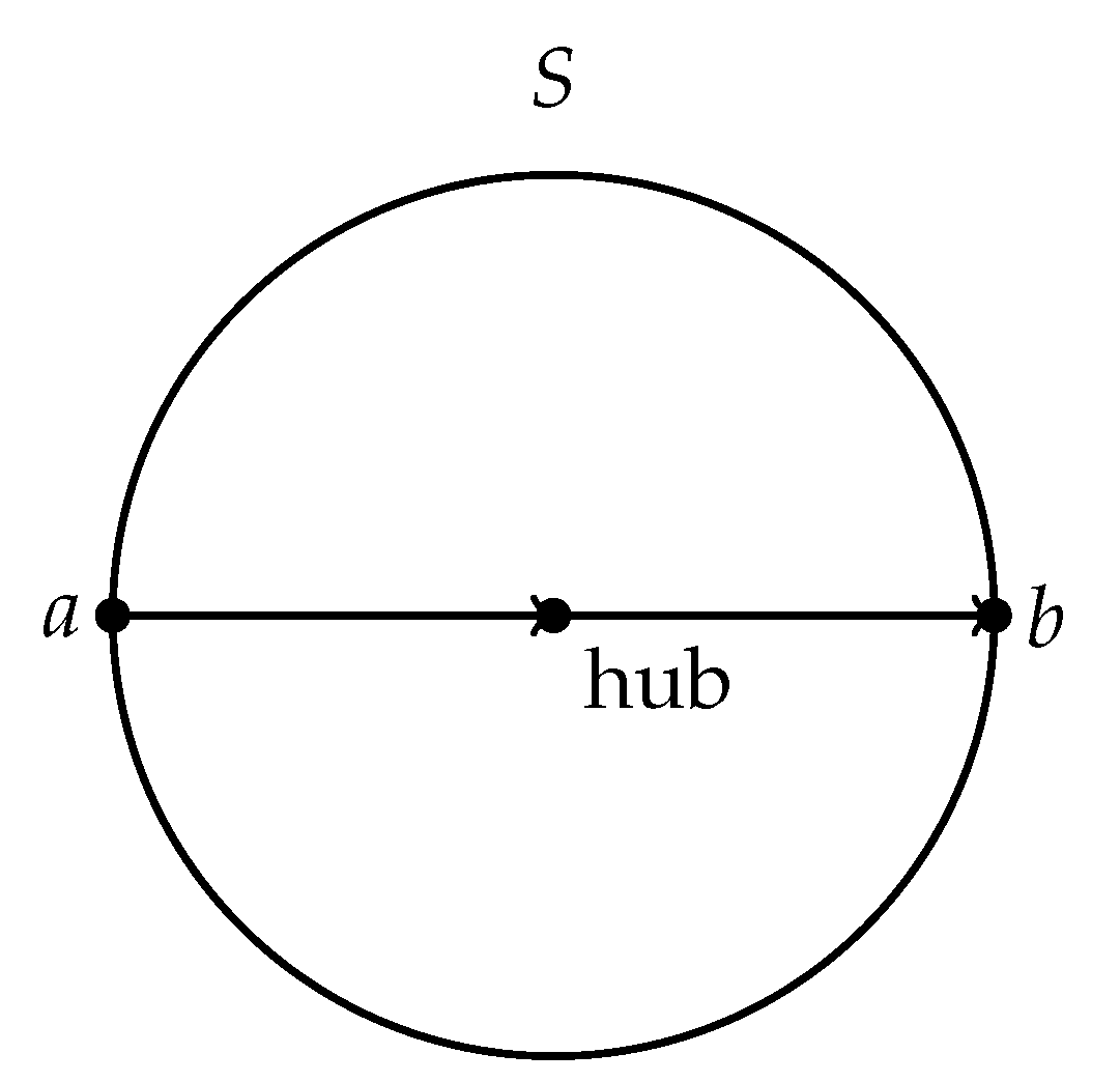
Figure 4.
Mechanistic integration model. Panel (a) shows the probability that a window is successful, meaning every required two-way exchange finishes before the window ends. The horizontal axis is , the ratio of best-case diameter-crossing time to the available window. Panel (b) is a robustness sweep. It repeats the same calculation while varying the number of sites N and the jitter level j. Here j is the mean random extra delay per message as a fraction of the window. It reports , the value of x where success probability is . Reference lines mark the theoretical thresholds for hub exchange and for all-to-all exchange.
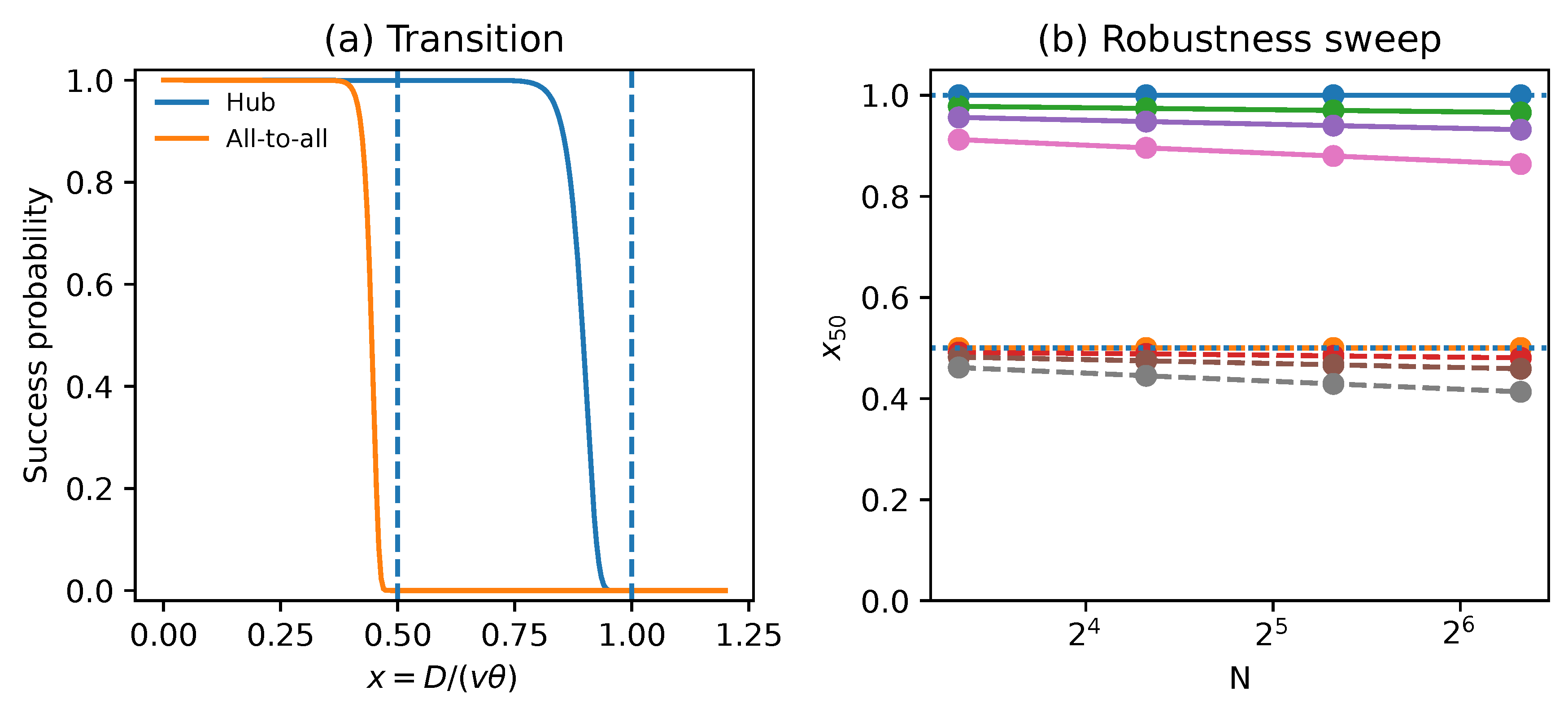
Figure 5.
Primate literature anchor. Dataset contains individuals from the corrected Phillips et al Table 1 [22]. Panel a shows the implied lower bound from published interhemispheric conduction time proxies (median and fast fibres) versus brain mass. Panel b shows, for a candidate window , the fraction of individuals whose reported conduction time would exceed that window.
Disclaimer/Publisher’s Note: The statements, opinions and data contained in all publications are solely those of the individual author(s) and contributor(s) and not of MDPI and/or the editor(s). MDPI and/or the editor(s) disclaim responsibility for any injury to people or property resulting from any ideas, methods, instructions or products referred to in the content. |
© 2026 by the author. Licensee MDPI, Basel, Switzerland. This article is an open access article distributed under the terms and conditions of the Creative Commons Attribution (CC BY) license.
Copyright: This open access article is published under a Creative Commons CC BY 4.0 license, which permit the free download, distribution, and reuse, provided that the author and preprint are cited in any reuse.


