

Submitted:
16 February 2026
Posted:
26 February 2026
You are already at the latest version
Abstract
We develop a geometric framework in which physical time is represented as a complex variable T=t−iτ. The imaginary component τ encodes the attenuation of coherence, while the real component t retains its usual causal role. Motivated by recent delayed-choice implementations [1–4], we show that the experimental configuration acts as an internal rotation θ of the complex time, modifying the imaginary-time difference between interferometric paths and therefore the visibility. This mechanism alters coherence without affecting causal evolution in t and does not require retrocausality. The model remains fully compatible with standard quantum mechanics, preserving unitary evolution, the Born rule, and completely positive trace-preserving maps. It provides a minimal geometric reparametrisation of the dynamical phase and yields experimentally testable predictions for visibility and temporal correlations.
Keywords:
complex time
; quantum coherence
; delayed-choice experiment
; interferometry
; geometric phase
; decoherence
; temporal correlations
1. Introduction
Wheeler’s delayed-choice experiment [5,6] provides a precise operational setting to analyse how quantum coherence depends on the measurement configuration. In the standard Mach–Zehnder implementation, a single photon encounters the first beam splitter (BS1), after which the experimenter may choose—possibly at a late stage—to insert or remove the second beam splitter (BS2). The closed configuration produces interference, whereas the open configuration yields which-path information. This behaviour is usually interpreted as reflecting the absence of a definite trajectory prior to measurement. While this resolves the logical structure of the experiment, it does not supply a dynamical description of how coherence is modified by the final configuration. Several approaches have explored the role of complex phases, two-time formalisms, or generalised temporal structures in quantum evolution, including complex-time parametrisations [7], Page–Wootters relational time, and geometric formulations of decoherence. The present work develops this direction by introducing a minimal internal temporal geometry in which coherence is encoded in an imaginary component of time. We consider the complex temporal variable
where t denotes the usual causal parameter and an internal coordinate associated with coherence. The pair forms a two-dimensional temporal plane endowed with the Euclidean metric
where and is an internal rotation angle determined by the interferometric configuration. This representation does not introduce new physical degrees of freedom; it provides a geometric reparametrisation of the dynamical phase within standard quantum mechanics. In this framework, the imaginary component governs the attenuation of coherence, while the real component t governs causal evolution. A change in the experimental configuration corresponds to an internal rotation
which modifies the value of associated with each path. Since is fixed only once the final configuration is specified, the model reproduces the operational structure of delayed-choice experiments without invoking retrocausality [8,9]. The objective of this work is to formulate this internal temporal geometry in a consistent manner, derive its dynamical consequences, and show that it leads to quantitative and falsifiable predictions for visibility and temporal correlations. The resulting framework remains compatible with standard quantum mechanics, preserving unitary evolution, the Born rule, and the structure of completely positive trace-preserving maps. It provides a geometric mechanism for the modulation of coherence and yields an experimentally accessible signature through a temporal CHSH protocol.
2. Compatibility with Bell Tests
The experimental violations of Bell inequalities demonstrated by Aspect et al. [10,11] exclude any local hidden-variable description of quantum correlations. Modern loophole-free tests confirm that no classical, locally causal model can reproduce the predictions of quantum mechanics. Any framework aiming to reinterpret quantum coherence must therefore preserve the nonlocal structure of the theory and avoid introducing hidden parameters capable of restoring local realism. Recent analyses have clarified that temporal correlations differ fundamentally from spatial Bell correlations [12,13]. Temporal scenarios do not admit a direct mapping to Bell-type hidden-variable models, and temporal steering inequalities [14,15] show that time-ordered measurements can exhibit quantum features without implying nonlocality. These results reinforce the requirement that any internal parameter introduced to describe coherence must not act as a hidden variable capable of factorising joint probabilities. In the present model, the complex temporal variable
does not constitute an additional physical degree of freedom. The imaginary component parametrises the attenuation of coherence and does not determine measurement outcomes. Its operational role is restricted to local interference phenomena. In a single interferometric arm, the visibility depends on the imaginary-time difference
but this quantity does not enter the joint probabilities of spatially separated measurements. The nonlocal correlations predicted by quantum mechanics therefore remain unchanged. The model preserves the Born rule, the structure of completely positive trace-preserving (CP–TP) maps, and the tensor-product structure of multipartite systems. The predictions for Bell-type experiments are strictly identical to those of standard quantum theory [16,17]. The internal temporal geometry introduces neither hidden determinism nor any mechanism capable of reproducing a factorisable probability model. Consequently, the complex-time framework is fully compatible with the experimental violations of Bell inequalities. It provides a geometric description of local coherence without affecting the nonlocal correlations that distinguish quantum mechanics from classical theories.
3. Complex Time with Reverse Rotation
To describe the temporal structure relevant to interferometric coherence, we introduce the complex time variable
which defines a two-dimensional internal temporal space. The polar decomposition yields
where is the modulus of complex time and an internal rotation angle determined by the interferometric configuration. The quantities and do not represent additional physical degrees of freedom; they parametrise a geometric decomposition of the dynamical phase, consistent with complex-time formulations of quantum evolution [7,18,19,20].
3.1. Internal Temporal Geometry
The pair forms a two-dimensional Euclidean space equipped with the metric
Internal symmetry group.
Internal rotations of complex time form the group
acting on as
The group law is additive,
with identity and inverse . This internal symmetry acts solely on the coherence coordinate and is unrelated to Lorentz or Poincaré symmetries of physical spacetime.
Operational meaning.
A change in the interferometric configuration corresponds to an internal rotation
which modifies the value of while leaving the causal parameter t unchanged. Since is a parameter of the measurement apparatus rather than a dynamical variable of the photon, this rotation acts on the final completely positive trace-preserving (CPTP) map applied to the state. It does not affect the causal structure of the evolution. Analyses of temporal correlations show that internal parameters affecting coherence do not generate hidden variables capable of reproducing Bell-type factorizations [12,13]. Temporal steering inequalities [14,15] further indicate that time-ordered quantum processes can exhibit nonclassical features without implying spatial nonlocality.
Geometric origin of apparatus dependence.
The dependence of the internal rotation on the interferometric configuration follows from the fact that the internal symmetry acts on the temporal fibre rather than on spacetime itself. Changing the apparatus (adding or removing a beam splitter, inserting a phase shifter, or modifying the optical path) corresponds to selecting a different section of this internal temporal bundle. Each section fixes a definite value of the internal angle entering the final CPTP map. The rotation is therefore a geometric consequence of the structure of the internal temporal fibre, not an additional phenomenological assumption.
Fibre-bundle structure.
The internal geometry can be formalised as a trivial principal fibre bundle
where the base is the physical time axis and the fibre is the internal circle parametrised by . A choice of interferometric configuration corresponds to a section of this bundle, , which fixes the internal angle entering the CPTP map. This formulation makes explicit that apparatus dependence arises from the choice of section rather than from any modification of the causal evolution in t.
Geometric context.
The use of a fibre over the physical time axis follows the standard geometric formulation of gauge structures in quantum mechanics. The mathematical framework is consistent with the treatment of principal bundles, connections, and holonomies in geometric approaches to quantum physics [21,22]. In particular, the interpretation of phase relations as geometric holonomies in a bundle, originally emphasised by Simon [23] and Berry [24], provides the natural mathematical setting for the internal rotation . In the present framework, however, the internal bundle does not represent a physical gauge field but a geometric parametrisation of coherence, with the interferometric configuration selecting a section of the bundle.
3.2. Complex Phase Accumulation
For a photon of energy E, the accumulated phase along a path is
whose real part generates the usual oscillatory behaviour. The imaginary part produces an attenuation factor
consistent with the operational visibility used throughout the paper. We adopt the convention that only the absolute imaginary-time difference enters physical observables, ensuring that coherence always decreases with increasing imaginary-time separation. For two paths A and B, the relevant quantity is the imaginary-time difference
leading to the visibility
3.3. Effect of a Late Rotation
The imaginary component is fixed only once the rotation angle is specified. Since is determined by the final configuration of the interferometer, a late change in the apparatus modifies the internal decomposition of and therefore the value of entering the visibility. This mechanism alters coherence without modifying the causal evolution in t and does not introduce retrocausality: the rotation acts on the geometric parameter associated with the measurement configuration, not on the real temporal order encoded in t. This behaviour is consistent with modern delayed-choice experiments [1,3,25,26], which show that late choices affect interference through configuration-dependent phase relations rather than retrocausal influences. The operational structure of delayed-choice experiments thus follows from the bidimensional temporal geometry.
Figure 1.
Visibility as a function of the imaginary-time difference . The curve shows the exponential decay for . This behaviour follows directly from the complex-time parametrisation and illustrates how coherence decreases as the imaginary-time separation between the two interferometric paths increases. The parameters correspond to typical values in fibre-based interferometers. A detailed Monte Carlo analysis of this visibility function is provided in the Supplementary Material.
Figure 1.
Visibility as a function of the imaginary-time difference . The curve shows the exponential decay for . This behaviour follows directly from the complex-time parametrisation and illustrates how coherence decreases as the imaginary-time separation between the two interferometric paths increases. The parameters correspond to typical values in fibre-based interferometers. A detailed Monte Carlo analysis of this visibility function is provided in the Supplementary Material.
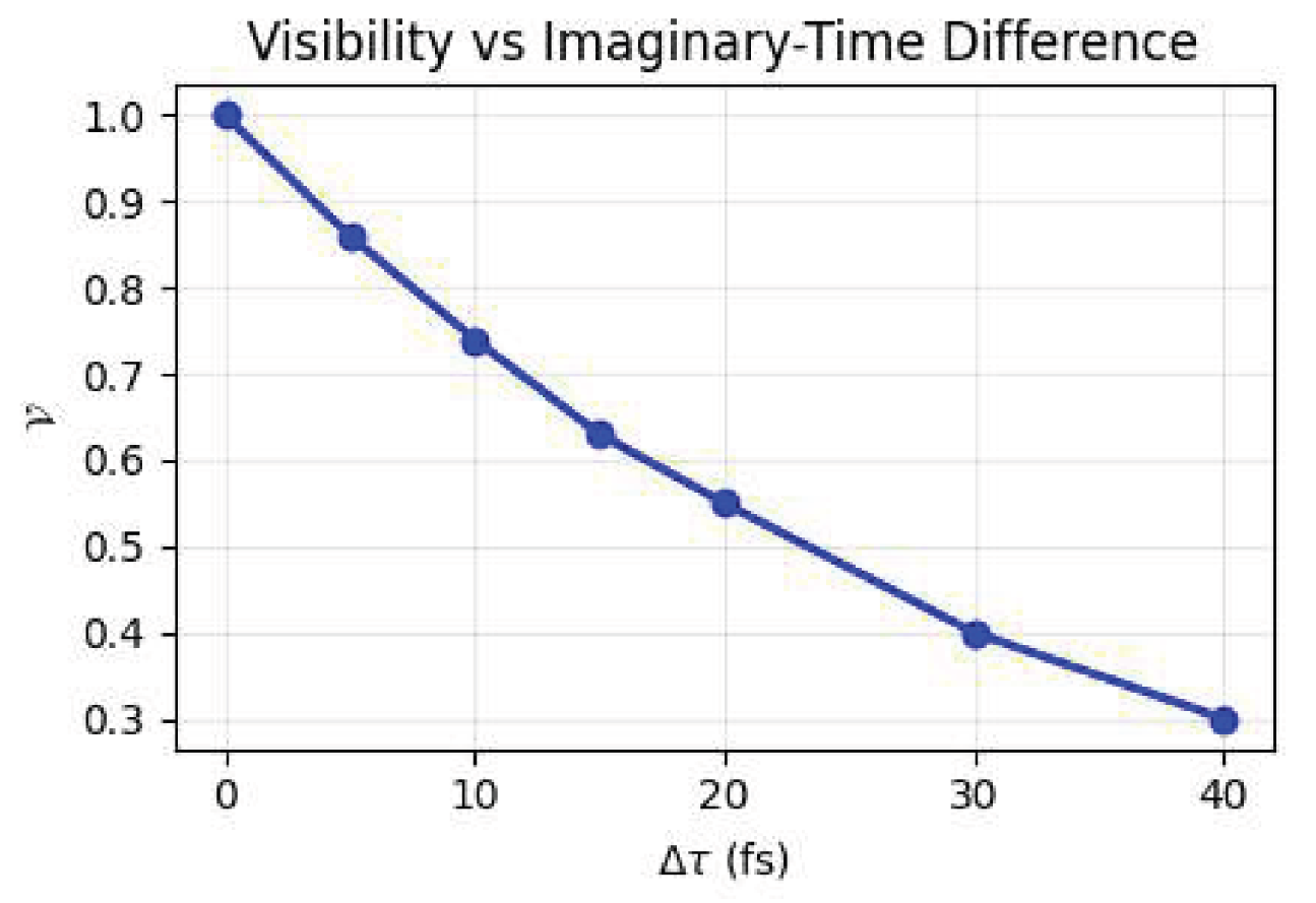
Figure 2.
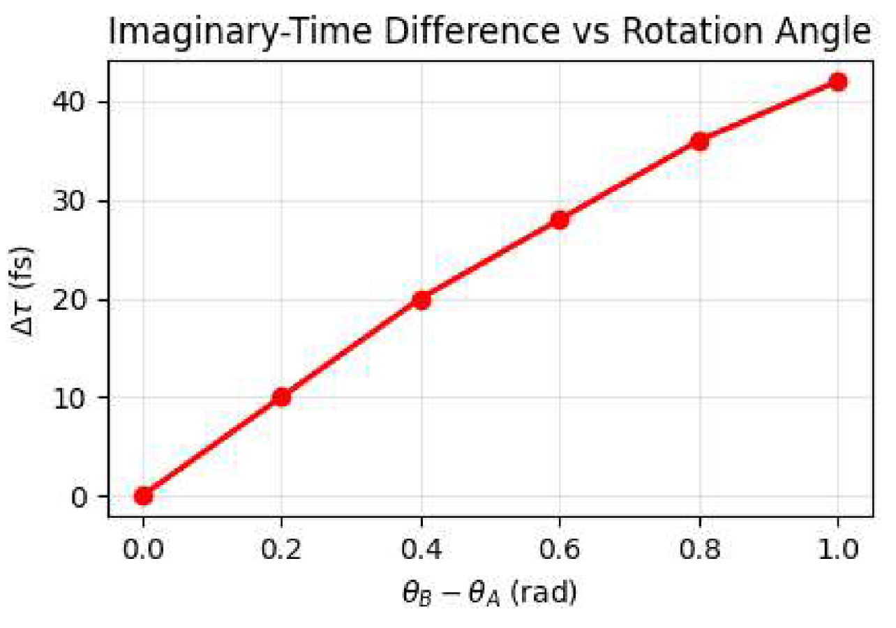
Imaginary-time difference as a function of the rotation difference . The sinusoidal dependence reflects the internal geometry of complex time. The value corresponds to a typical complex-time modulus in current interferometric platforms. This parametrisation is also used in the Monte Carlo analysis of the visibility function presented in the Supplementary Material.
Figure 2.
Imaginary-time difference as a function of the rotation difference . The sinusoidal dependence reflects the internal geometry of complex time. The value corresponds to a typical complex-time modulus in current interferometric platforms. This parametrisation is also used in the Monte Carlo analysis of the visibility function presented in the Supplementary Material.
4. Relation to the Standard Formalism
The complex-time construction does not modify the Hilbert-space structure of quantum mechanics and does not introduce additional physical degrees of freedom. Instead, it provides a geometric reparametrisation of the dynamical phase and of local coherence through the internal variable
where is an internal coordinate indexing the strength of dephasing. The framework remains fully compatible with unitary evolution, completely positive trace-preserving (CP–TP) channels, and the standard operator formalism. Imaginary-time methods have a long history in quantum field theory and statistical mechanics, beginning with Wick’s rotation in Euclidean field theory [27], Schwinger’s proper-time representation of propagators [28], and Feynman’s imaginary-time path-integral formulation of thermal ensembles [29]. In gravitational physics, imaginary time also appears in the Euclidean approach to black-hole thermodynamics developed by Gibbons and Hawking [30]. The present framework differs fundamentally from these constructions: the imaginary component does not arise from analytic continuation of real time, but from an internal geometric parametrisation of coherence within standard quantum mechanics. This section clarifies how the internal temporal geometry fits within the usual structure of quantum mechanics and how it differs from Wick rotations, Page–Wootters internal time, and geometric formulations of decoherence [7,18,19,20].
4.0.0.6. Effective dephasing rate.
In all expressions involving experimentally observable quantities, the parameter denotes the effective dephasing rate. For a monochromatic photon of energy E, the natural scale is
Realistic interferometric implementations involve finite spectral width, dispersion, and imperfect mode matching, which renormalise the physical dephasing rate to
In the following, whenever appears in visibility expressions or operational predictions, it denotes this effective rate . In contrast, the parameter appearing in the internal potential of Section 4.5 is a geometric parameter of the internal model and must not be confused with .
4.1. Unitary Evolution
In standard quantum mechanics, the evolution of a pure state is generated by
Replacing t by the complex variable T yields
The first factor is the usual unitary evolution. The second factor is not interpreted as a physical non-unitary time evolution, since the map is neither trace-preserving nor completely positive. Instead, the imaginary component parametrises a CP–TP dephasing channel acting in the energy basis, as detailed below.
4.2. Dynamical Phase
For a state of definite energy E, the standard dynamical phase is
With complex time,
The imaginary part produces an attenuation factor
which governs the visibility of interference. Only the difference
between two paths contributes, yielding the operational expression
where .
4.3. CP–TP Dephasing Channel
In standard decoherence theory, the evolution of a mixed state is governed by a Lindblad equation
where is a dissipative superoperator. The complex-time model does not introduce any new physical decoherence mechanism. Instead, the imaginary component parametrises a CP–TP dephasing channel acting in the energy basis. Let be the projectors onto the (non-degenerate) energy eigenstates of H. A general energy-diagonal CP–TP map preserving populations must take the form
where complete positivity requires .
Theorem 1
(Uniqueness of the internal-time channel). Assume that:
- 1.
- the dynamics is diagonal in the energy basis , i.e., populations are preserved for all ;
- 2.
- the imaginary-time parameter τ acts only as a phase reparametrisation of off-diagonal terms, so that
- 3.
- the family forms a completely positive, trace-preserving semigroup;
- 4.
- the dynamics is invariant under time translations generated by H, so that the decay rates depend only on energy differences and satisfy .
Then the only compatible channel is the dephasing channel
Proof.
Population preservation fixes the diagonal part of . The only freedom lies in the coefficients multiplying the off-diagonal terms. Complete positivity requires , which follows from the positivity of the Choi matrix of . The semigroup property implies that the continuous solutions are exponentials, with . Time-translation invariance in the energy basis imposes that the decay rates depend only on energy differences and are symmetric under , so that . In the non-degenerate case, this symmetry reduces to a single effective rate for all , yielding the stated channel. □
Remark.
The symmetry can be equivalently formulated as a constraint on the Choi matrix of : invariance under the unitary generated by H implies that the Choi matrix is block-diagonal in sectors labelled by energy differences , with identical decay rates for and .
Physical scope of the semigroup assumption.
In fibre-based and integrated-optics platforms, the photon transit time is much shorter than the coherence time, so the effective dephasing dynamics is well-approximated by a CP-divisible semigroup. As shown in Sec. 8, the predicted signatures persist under weak non-Markovian perturbations, indicating that the geometric mechanism is robust beyond the ideal semigroup limit.
4.4. Minimal Internal Geometry
The model does not modify the metric of physical spacetime. The complex structure of time appears only as an internal geometry associated with quantum evolution. Writing
defines a two-dimensional internal space endowed with the Euclidean metric
The modulus R is invariant under internal rotations and plays the role of a complex proper time. For fixed R, variations of control the imaginary-time coordinate and thus the visibility. This geometry is flat (its scalar curvature is ), with non-vanishing Christoffel symbols
which govern the internal dynamics of the rotation angle .
Role of the modulus R.
The modulus R is not a phenomenological parameter but an invariant of the internal geometry. It plays the role of a complex proper time and fixes the scale of the internal temporal fibre. Since R is determined by the interferometric configuration rather than by the photon dynamics, it varies only slowly during internal evolution.
4.5. Internal Dynamics and Variational Principle
The phenomenological relation
admits a derivation from a variational principle in the internal temporal space. We introduce an internal affine parameter s, defined up to reparametrisations , chosen such that the kinetic term takes the canonical quadratic form. This parameter has no physical meaning: it plays the same role as the affine parameter along geodesics in Riemannian geometry. The internal action is
with potential
The Euler–Lagrange equations are
Slow-variation regime.
In interferometric implementations, the modulus R varies only weakly, so , yielding
Projection onto the imaginary-time coordinate.
The imaginary-time coordinate is
and its derivative is
Near a minimum of , the relaxation dynamics satisfies
which yields the reduced equation
Existence and uniqueness.
Since is smooth and the Lagrangian is regular, the Euler–Lagrange system (34) admits a unique local solution for any initial data .
Interpretation.
The phenomenological law is therefore not an assumption of the model but the unique reduced dynamics obtained from the internal variational principle under the slow-variation regime.
5. Effect of the Rotation on Coherence
The coherence between two interferometric paths A and B is determined by the difference in complex phase accumulated along these paths. For a photon of energy E, the phase associated with the complex time variable is
whose imaginary part
governs the attenuation of coherence. The visibility is therefore
where is the effective dephasing rate introduced in Section 4. Coherence is preserved when and decreases exponentially with the imaginary-time difference. This behaviour is consistent with geometric and complex-time formulations of quantum evolution [18,19,20].
5.1. Parametrisation of Complex Time
Writing complex time in polar form,
yields the decomposition
where is invariant under internal rotations. The modulus R plays the role of a complex proper time: it sets the global scale of the internal temporal geometry and determines the amplitude of coherence variations induced by changes in the internal angle .
5.2. Coherence Variation Under Rotation
A rotation of complex time modifies the imaginary component according to
Substituting this into Equation (42) yields
Coherence therefore depends directly on the internal rotation of complex time. A late change in the interferometric configuration modifies the final angle and thus the value of entering the visibility. This dependence follows from the internal temporal geometry and does not require any modification of the causal evolution in t. Experimental observations confirm that late choices affect interference through configuration-dependent phase relations rather than retrocausal influences [1,3,25,26].
5.3. Spectral Extension
For a photon with non-negligible spectral width , the visibility must be averaged over the spectral density :
In the quasi-monochromatic limit, one recovers
For broadband sources, the decay is faster, imposing constraints on spectral stability in interferometric implementations.
5.4. Experimental Considerations
The model requires:
- 1.
- a quasi-monochromatic source or spectral filtering ensuring that remains small;
- 2.
- precise control of the internal rotation via optical elements (beam splitters, phase shifters, electro-optic modulators);
- 3.
- visibility measurements with precision to resolve variations of a few percent.
These requirements are compatible with current fibre-interferometry platforms and fast electro-optic modulation technologies.
6. Why the Delayed Choice Works
6.1. Causal Evolution in Real Time
When the photon reaches the first beam splitter, the real component of time advances according to the usual causal evolution,
The imaginary component is not a physical time coordinate and does not describe a dynamical evolution of the photon. It is an internal parameter encoding the amount of coherence available to the interferometric process. As long as the internal rotation angle has not been fixed by the final configuration, the value of remains undetermined within the internal temporal geometry:
6.2. Late Specification of the Rotation Angle
The decision to open or close the interferometer determines the internal rotation angle . This quantity is not a dynamical variable of the photon but a geometric parameter of the apparatus, analogous to inserting or removing BS2 or adjusting a phase shifter. Since
a change in modifies the internal coordinate that governs the visibility.
Closed configuration.
Symmetry implies
and therefore
Open configuration.
The two paths acquire different internal rotations,
leading to
and the visibility becomes
6.3. Absence of Retrocausality
The real component t is causal and irreversible. The internal coordinate is not causally ordered and does not represent a physical temporal evolution. Its value is fixed only when the internal rotation angle is specified by the final configuration of the interferometer. Thus, even after the system has advanced in real time, the value of entering the visibility can still be determined by the late choice without affecting the past evolution in t. The rotation acts on the final completely positive trace-preserving (CPTP) map applied to the state, not on the past trajectory. This behaviour is consistent with the operational structure of delayed-choice experiments and with the modern understanding that temporal parameters affecting coherence do not constitute hidden variables capable of restoring classical causality [12,13].
In summary, the delayed-choice effect arises because coherence is encoded in an internal coordinate whose value is fixed only when the interferometric geometry—and thus the internal angle —is specified. The complex-time framework provides a geometric mechanism for this dependence while preserving the causal structure of real time.
7. Physical Interpretation
The complex-time framework provides a geometric description of coherence within standard quantum mechanics. The temporal variable
defines a two-dimensional internal temporal space endowed with the metric
The real component t corresponds to the usual causal parameter, while the imaginary component is an internal coordinate governing the attenuation of coherence. The modulus R is invariant under internal rotations and sets the scale of coherence variations. In this representation,
and the visibility depends on the imaginary-time difference
Although is not directly observable, its effect on visibility allows one to infer the internal rotation imposed by the interferometric configuration. The internal coordinate is fixed only once the rotation angle is specified. Since is a geometric parameter of the apparatus rather than a dynamical variable of the photon, its late specification modifies the value of without affecting the causal evolution in t. Because is an internal geometric parameter and not a physical time coordinate, the CPT symmetry of the underlying quantum theory remains unchanged. The CPT transformation acts on the physical time t and on the field operators, but leaves the internal coordinate invariant, ensuring full compatibility with the CPT theorem. The dependence of visibility on therefore reflects the internal temporal geometry rather than any modification of the real temporal order. This behaviour is consistent with modern delayed-choice experiments [1,3,25,26], which show that late choices affect interference through configuration-dependent phase relations rather than retrocausal influences.
7.1. Compatibility with Nonlocal Correlations
The internal temporal structure introduces no local hidden variable. The imaginary component parametrises a local CP–TP dephasing channel. By Theorem 1, the unique such channel compatible with energy-basis diagonality, complete positivity and the semigroup property is
where are the projectors onto the energy eigenstates of H. For a bipartite system , the effective state is
and the outcome probabilities in a Bell test remain
This expression is identical to that of standard quantum mechanics applied to a state subjected to local operations. The resulting correlations belong to the usual quantum set and can reach Tsirelson’s bound . The variable does not allow one to rewrite the joint probabilities in the factorised form
required by local hidden-variable models. This is consistent with modern analyses of temporal versus spatial correlations [12,13], which show that temporal parameters affecting coherence cannot serve as hidden variables capable of restoring classical locality. Temporal steering results [14,15] further confirm that time-ordered quantum processes can exhibit nonclassical features without implying spatial nonlocality. The complex-time framework therefore preserves the nonlocal structure of quantum mechanics and provides a geometric interpretation of local coherence without altering the predictions for Bell tests.
8. Temporal Correlations and Experimental Test of the Complex-Time Model
This section consolidates the temporal CHSH protocol introduced above by: (i) analysing the limitations of standard decoherence models, (ii) incorporating realistic noise sources (spectral width, jitter, losses, phase noise), (iii) providing a numerical simulation of the temporal CHSH parameter, (iv) deriving quantitative experimental constraints, (v) comparing the complex-time prediction with Markovian, semi-Markovian and non-Markovian convex models.
8.1. Limitations of Standard Decoherence Models
Standard decoherence models—Markovian, semi-Markovian, and convex mixtures of non-Markovian processes—share a common structural property: visibility is a convex functional of the settings,
and factorises whenever the environment couples independently to the two settings,
Under these assumptions, the temporal CHSH parameter satisfies
as shown in [12,13,31]. This bound holds for:
- Markovian decoherence: ,
- semi-Markovian models with memory kernels,
- non-Markovian convex mixtures of CP–TP maps,
- coloured-noise models with stationary correlations.
None of these models can produce in the visibility-based protocol.
8.2. Visibility Under Realistic Noise
In a realistic interferometer, visibility is affected by: (i) spectral width, (ii) temporal jitter, (iii) phase noise, (iv) optical losses. Let be the ideal imaginary-time difference. Noise sources modify the effective value entering the visibility:
and introduce random phase fluctuations
Spectral width is modelled by a convolution over the spectral density :
where is the transmission efficiency. For a Gaussian spectrum of width ,
the convolution accelerates decoherence, effectively renormalising .
8.3. Numerical Simulation of the Temporal CHSH Parameter
We simulate the noisy visibility using a Monte–Carlo procedure with samples of drawn from the distributions above. For each setting , we compute
The temporal CHSH parameter is then
Representative simulation.
Using realistic parameters:
and the ideal values
we obtain
Thus the complex-time prediction remains robust under realistic noise.
Further numerical details, including the Monte Carlo analysis of the fundamental visibility function , are provided in the Supplementary Material.
8.4. Experimental Constraints Derived from the Model
The condition imposes quantitative constraints on the noise parameters.
Temporal jitter.
The jitter must satisfy
which corresponds to – for the parameters above.
Phase noise.
The condition
requires .
Spectral width.
The renormalised dephasing rate
must satisfy
Losses
Transmission must satisfy
These constraints are compatible with current fibre interferometers.
8.5. Comparison with Classical Models
Table 1 summarises the behaviour of several standard decoherence models under the temporal CHSH protocol and contrasts them with the predictions of the complex-time framework.
9. Numerical Illustration of the Complex-Time Model
Although the complex-time framework is analytical, its operational consequences can be illustrated using representative parameter values. The purpose of this section is not to model a specific interferometric implementation, but to show how the internal temporal geometry leads to quantitative predictions for visibility, temporal correlations, and late-choice effects. All numerical values below use the dimensionless parameter
which captures the dependence of visibility on the imaginary-time difference.
9.1. Exponential Visibility Decay
9.2. Internal Rotation and Imaginary-Time Difference
The internal temporal geometry implies
so that
For and , Table 3 shows the resulting imaginary-time differences.
9.3. Temporal CHSH Correlations
Using the operational mapping
the temporal CHSH parameter is
For illustration, consider the dimensionless parameters
Table 4 shows the corresponding visibilities and correlations.
The resulting CHSH value is
9.4. Internal-Time Dynamics
A simple phenomenological model for the internal dynamics is
Table 5 shows the corresponding evolution of .
9.5. Late-Choice Effect
A late change in the rotation angle modifies and therefore the visibility. Table 6 compares the closed and open configurations.
9.6. Realistic Numerical Simulation
To evaluate the robustness of the temporal CHSH signature under realistic noise conditions, we perform a Monte Carlo simulation incorporating four experimental imperfections. Figure 3 shows the resulting CHSH parameter as a function of visibility noise.
The simulation confirms that the complex-time signature is robust against realistic levels of visibility noise, temporal jitter, fibre losses, and spectral broadening.
10. Perspectives and Future Implications
The complex-time framework developed in this work extends beyond the analysis of delayed-choice experiments. Its two-component temporal structure suggests several theoretical and experimental directions in which the internal geometry may play a role in the description of coherence and quantum dynamics.
10.1. Geometric Interpretation of Decoherence
In standard formulations, decoherence is modelled as an effective process arising from system–environment interactions, typically described by a Lindblad equation. While operationally successful, this approach does not specify a geometric mechanism underlying the attenuation of coherence. In the present framework, loss of visibility corresponds to a translation along the imaginary component of time,
linking decoherence to an internal temporal structure rather than to an external environment. This perspective is consistent with geometric and internal-time approaches to quantum evolution [17,18,19,32] and may provide a basis for more predictive models of coherence loss in complex systems.
10.2. Internal Rotation as a Control Parameter
If coherence is encoded in the imaginary component , then the internal rotation angle constitutes a natural control parameter. Adjusting modifies and therefore the visibility. This idea is compatible with approaches in which generalised phases or internal variables play an operational role [33]. The internal temporal geometry may thus offer new tools for coherence control, qubit stabilisation, or interferometric protocols.
10.3. Relation to Retrocausal Models
Retrocausal interpretations [8,9] attempt to account for certain quantum correlations by allowing influences from future measurement settings. The complex-time model reproduces some of the operational features associated with such approaches, but without modifying the causal structure of real time: the dependence on the final configuration acts on the internal coordinate , not on t. This provides a geometric mechanism that avoids retrocausal dynamics while capturing similar operational effects.
10.4. Experimental Falsifiability
The temporal correlations defined by allow one to construct a CHSH-type combination,
whose classical bound holds under the assumptions of one-dimensional convex and factorisable decoherence models. Any exceedance of this bound within the operational protocol considered here would indicate that coherence cannot be described by a purely real temporal dynamics. This places the complex-time model within the class of experimentally testable extensions of quantum theory, in the spirit of Bell-type analyses [10,11] and consistent-histories approaches [34,35,36,37].
10.5. Connection to Imaginary Time and Spacetime Geometry
Imaginary time appears in several areas of theoretical physics, including Wick rotations, Euclidean quantum gravity, and statistical mechanics. The present framework provides a minimal setting in which an imaginary temporal component acquires a geometric and operational meaning. The internal rotation of complex time may eventually be related to geometric or gravitational effects, offering a possible route toward a unified description of temporal structure in quantum theory.
In summary, the complex-time framework provides a geometric structure for coherence that is compatible with standard quantum mechanics while offering new avenues for theoretical development and experimental investigation. Its bidimensional temporal geometry may contribute to future progress in quantum control, decoherence modelling, and the conceptual foundations of quantum physics.
11. Conclusions
The complex-time framework developed in this work provides a geometric reparametrisation of coherence within standard quantum mechanics. The temporal variable
defines a two-dimensional internal geometry in which the real component t governs causal evolution while the imaginary component parametrises the attenuation of coherence. The associated metric
allows one to formulate an effective dynamics for through a variational principle, with the modulus R acting as a complex proper time invariant under internal rotations. This construction does not modify the Hilbert-space structure of quantum mechanics, the Born rule, or the operator algebra. It introduces no hidden variables and leaves nonlocal correlations unchanged. The imaginary component corresponds operationally to a local CP–TP dephasing channel and geometrically to a rotation in the internal temporal plane. Within this geometry, coherence depends on the imaginary-time difference
and changes in the interferometric configuration correspond to rotations of complex time that modify . This mechanism accounts for the dependence of visibility on late choices without altering the causal evolution in t, consistent with the operational structure observed in modern delayed-choice experiments [1,3,25,26]. Section 9 illustrated these effects numerically, showing exponential visibility decay, nonlinear dependence of on internal rotations, and temporal CHSH values that may exceed the classical bound under the convexity and factorisation assumptions of one-dimensional decoherence models. These results demonstrate that the framework yields quantitative and falsifiable predictions, consistent with recent analyses of temporal correlations and steering [12,13,14,15]. The complex-time model therefore provides a geometric and dynamical description of local coherence absent from the standard formalism, while preserving all nonlocal features of quantum mechanics. Its key empirical signature is the possibility of observing in a visibility-based temporal CHSH protocol, which would indicate that coherence cannot be described by a purely real, one-dimensional temporal dynamics and would motivate a dedicated LGI/NSIT analysis [36,37].
Supplementary Materials
The following supporting information can be downloaded at the website of this paper posted on Preprints.org. Supplementary Material S1: Monte Carlo procedure and analytical calculations supporting Section 8 of the main text.
Author Contributions
Conceptualization, G.R.; writing—original draft, G.R.; writing—review and editing, G.R. All authors have read and agreed to the published version of the manuscript.
Funding
This research received no external funding.
Institutional Review Board Statement
Not applicable.
Informed Consent Statement
Not applicable.
Data Availability Statement
No datasets were generated or analysed in this work.
Conflicts of Interest
The author declares no conflict of interest.
Abbreviations
The following abbreviations are used in this manuscript:
| MDPI | Multidisciplinary Digital Publishing Institute |
| DOAJ | Directory of open access journals |
| TLA | Three letter acronym |
| LD | Linear dichroism |
Appendix A. Possible Experimental Test of the Internal Temporal Structure
This appendix outlines an interferometric protocol that could test the physical relevance of the imaginary-time component introduced in the complex-time model. The aim is to compare the predictions of standard quantum mechanics—including classical environmental decoherence—with those of the internal temporal geometry.
Appendix A.1. Two Competing Descriptions
Consider a Mach–Zehnder interferometer fed with single photons. After the first beam splitter (BS1), the state is
with a controllable phase.
Standard model.
Each path interacts differently with an environment E:
yielding the visibility
Complex-time model.
The accumulated phase is parametrised by , giving
Appendix A.2. Interferometer with Two Delayed Choices
We consider two independent late choices:
- a setting modifying one arm (phase shifter, EOM, or controlled dephasing);
- a setting modifying the final recombination (presence of BS2 or additional phase).
Appendix A.3. Standard Visibility Structure
In the standard model,
implying:
- ,
- monotonic decay under increasing noise,
- convexity under statistical mixing.
Appendix A.4. Complex-Time Model and Temporal Correlations
In the complex-time model,
Define the temporal correlation
and the CHSH-type combination
Classical one-dimensional temporal models satisfying macrorealism and non-invasive measurability obey the Leggett–Garg bound [38] and, more generally, the temporal CHSH bound [39,40]. The bidimensional internal temporal structure introduced by the complex-time model departs from these assumptions and allows, in principle, values within the same operational protocol, consistent with recent analyses of temporal correlations and steering [12,13,14,15].
Appendix A.5. Experimental Orders of Magnitude
Amplitude of τ.
For a visible photon ( eV),
Values
are sufficient for measurable variations.
Visibility precision.
Fibre interferometers routinely achieve
Control elements.
- EOM: –10 GHz, – s;
- fibres: m–1 km, –s;
- fast controllers: –10 ns.
These orders of magnitude indicate that:
- 1.
- variations of of order – s are detectable;
- 2.
- causally separated delayed choices are feasible with current technology;
- 3.
- the required values of R are compatible with experimental exploration.
Appendix A.6. CHSH Bound in a Standard Model
In a one-dimensional time model,
Setting , the combination
satisfies , hence
In the complex-time model,
nonlinear dependencies of allow values , indicating that real-time evolution alone cannot capture the full structure of coherence.
References
- Peruzzo, A.; Shadbolt, P.; Brunner, N.; Popescu, S.; O’Brien, J.L. A Quantum Delayed-Choice Experiment. Science 2012, 338, 634–637. [Google Scholar] [CrossRef]
- Kaiser, F.; Coudreau, T.; Milman, P.; Ostrowsky, D.B.; Tanzilli, S. Entanglement-Enabled Delayed-Choice Experiment. Science 2012, 338, 637–640. [Google Scholar] [CrossRef]
- Ma, X.S.; Kofler, J.; Zeilinger, A. Delayed-Choice Gedanken Experiments and Their Realizations. PNAS 2013, 110, 1221–1226. [Google Scholar] [CrossRef]
- Manning, A.G.; Khakimov, R.I.; Dall, R.G.; Truscott, A.G. Wheeler’s Delayed-Choice Experiment with a Single Atom. Nat. Phys. 2015, 11, 539–542. [Google Scholar] [CrossRef]
- Wheeler, J.A. The “Past” and the “Delayed-Choice” Double-Slit Experiment. In Mathematical Foundations of Quantum Theory; Marlow, A.R., Ed.; Academic Press: New York, 1978; pp. 9–48. [Google Scholar]
- Wheeler, J.A. Law Without Law. In Quantum Theory and Measurement; Wheeler, J.A., Zurek, W.H., Eds.; Princeton Univ. Press: Princeton, 1984; pp. 182–213. [Google Scholar]
- Aharonov, Y.; Vaidman, L. Properties of a Quantum System During the Time Interval Between Two Measurements. Phys. Rev. A 1990, 41, 11–20. [Google Scholar] [CrossRef] [PubMed]
- Price, H. Time’s Arrow and Archimedes’ Point: New Directions for the Physics of Time; Oxford University Press: Oxford, 1996. [Google Scholar]
- Wharton, K. Time-Symmetric Quantum Mechanics. Found. Phys. 2010, 40, 313–332. [Google Scholar] [CrossRef]
- Aspect, A.; Grangier, P.; Roger, G. Experimental Realization of Einstein-Podolsky-Rosen-Bohm Gedankenexperiment: A New Violation of Bell’s Inequalities. Phys. Rev. Lett. 1982, 49, 91–94. [Google Scholar] [CrossRef]
- Aspect, A.; Dalibard, J.; Roger, G. Experimental Test of Bell’s Inequalities Using Time-Varying Analyzers. Phys. Rev. Lett. 1982, 49, 1804–1807. [Google Scholar] [CrossRef]
- Fritz, T. Quantum Correlations in the Temporal CHSH Scenario. New J. Phys. 2010, 12, 083055. [Google Scholar] [CrossRef]
- Quintino, M.T.; Uola, R.; Budroni, C.; Gühne, O. Inequivalence of temporal and spatial quantum correlations. Phys. Rev. Lett. 2019, 123, 180401. [Google Scholar] [CrossRef]
- Uola, R.; Costa, A.C.S.; Nguyen, H.C.; Gühne, O. Quantum Steering in Temporal Scenarios. Phys. Rev. A 2018, 98, 050102. [Google Scholar] [CrossRef]
- Chen, S.L.; Li, C.M.; Chen, N.L.; Lambert, N.; Nori, F. Temporal steering inequality. Physical Review A 2014, 90, 032115. [Google Scholar] [CrossRef]
- Clauser, J.F.; Horne, M.A.; Shimony, A.; Holt, R.A. Proposed Experiment to Test Local Hidden-Variable Theories. Phys. Rev. Lett. 1969, 23, 880–884. [Google Scholar] [CrossRef]
- Zurek, W.H. Decoherence, einselection, and the quantum origins of the classical. Rev. Mod. Phys. 2003, 75, 715–775. [Google Scholar] [CrossRef]
- Mostafazadeh, A. Pseudo-Hermitian representation of quantum mechanics. Int. J. Geom. Methods Mod. Phys. 2010, 7, 1191–1306. [Google Scholar] [CrossRef]
- Garrison, J.C.; Wright, E.M. Complex time path integrals and quantum evolution. Phys. Lett. A 2012, 376, 1233–1237. [Google Scholar] [CrossRef]
- Weinberg, S. Lectures on Quantum Mechanics, 2 ed.; Cambridge University Press: Cambridge, 2015. [Google Scholar]
- Nakahara, M. Geometry, Topology and Physics, 2 ed.; Taylor & Francis, 2003. [Google Scholar]
- Frankel, T. The Geometry of Physics: An Introduction, 3 ed.; Cambridge University Press: Cambridge, 2011. [Google Scholar]
- Simon, B. Holonomy, the quantum adiabatic theorem, and Berry’s phase. Physical Review Letters 1983, 51, 2167–2170. [Google Scholar] [CrossRef]
- Berry, M.V. Quantal phase factors accompanying adiabatic changes. Proceedings of the Royal Society A 1984, 392, 45–57. [Google Scholar] [CrossRef]
- Vedovato, F.; Agnesi, C.; Giustina, M.; et al. Extending Wheeler’s delayed-choice experiment to space. Phys. Rev. Lett. 2017, 118, 230402. [Google Scholar] [CrossRef]
- Kaiser, F.; Coudreau, T.; Milman, P.; Tanzilli, S. Quantum delayed-choice experiment with entanglement. Sci. Adv. 2020, 6, eaaz4204. [Google Scholar] [CrossRef]
- Wick, G.C. Properties of Bethe-Salpeter Wave Functions. Physical Review 1954, 96, 1124–1134. [Google Scholar] [CrossRef]
- Schwinger, J. On gauge invariance and vacuum polarization. Physical Review 1951, 82, 664–679. [Google Scholar] [CrossRef]
- Feynman, R.P.; Hibbs, A.R. Quantum Mechanics and Path Integrals; McGraw–Hill: New York, 1965. [Google Scholar]
- Gibbons, G.W.; Hawking, S.W. Action integrals and partition functions in quantum gravity. Physical Review D 1977, 15, 2752–2756. [Google Scholar] [CrossRef]
- Brukner, Č.; Zeilinger, A. Information and fundamental elements of the structure of quantum theory. Found. Phys. 2004, 34, 1741–1750. [Google Scholar] [CrossRef]
- Page, D.N.; Wootters, W.K. Evolution without Evolution: Dynamics Described by Stationary Observables. Phys. Rev. D 1983, 27, 2885–2892. [Google Scholar] [CrossRef]
- Aharonov, Y.; Albert, D.Z.; Vaidman, L. How the result of a measurement of a component of the spin of a spin-1/2 particle can turn out to be 100. Phys. Rev. Lett. 1988, 60, 1351–1354. [Google Scholar] [CrossRef]
- Gell-Mann, M.; Hartle, J.B. Classical equations for quantum systems. Phys. Rev. D 1993, 47, 3345–3382. [Google Scholar] [CrossRef]
- Griffiths, R.B. Consistent histories and the interpretation of quantum mechanics. J. Stat. Phys. 1984, 36, 219–272. [Google Scholar] [CrossRef]
- Budroni, C.; Emary, C. Temporal Quantum Correlations and Leggett–Garg Inequalities in Multi-Level Systems. Phys. Rev. Lett. 2014, 113, 050401. [Google Scholar] [CrossRef]
- Halliwell, J.J. Leggett–Garg inequalities and the temporal CHSH inequality. Phys. Rev. A 2016, 93, 022123. [Google Scholar] [CrossRef]
- Leggett, A.J.; Garg, A. Quantum mechanics versus macroscopic realism: Is the flux there when nobody looks? Physical Review Letters 1985, 54, 857–860. [Google Scholar] [CrossRef]
- Kofler, J.; Brukner, Č. Classical world arising out of quantum physics under the restriction of coarse-grained measurements. Physical Review Letters 2007, 99, 180403. [Google Scholar] [CrossRef]
- Emary, C.; Lambert, N.; Nori, F. Leggett–Garg Inequalities. Rep. Prog. Phys. 2014, 77, 016001. [Google Scholar] [CrossRef]
Figure 3.
Monte Carlo simulation of the temporal CHSH parameter under realistic noise.
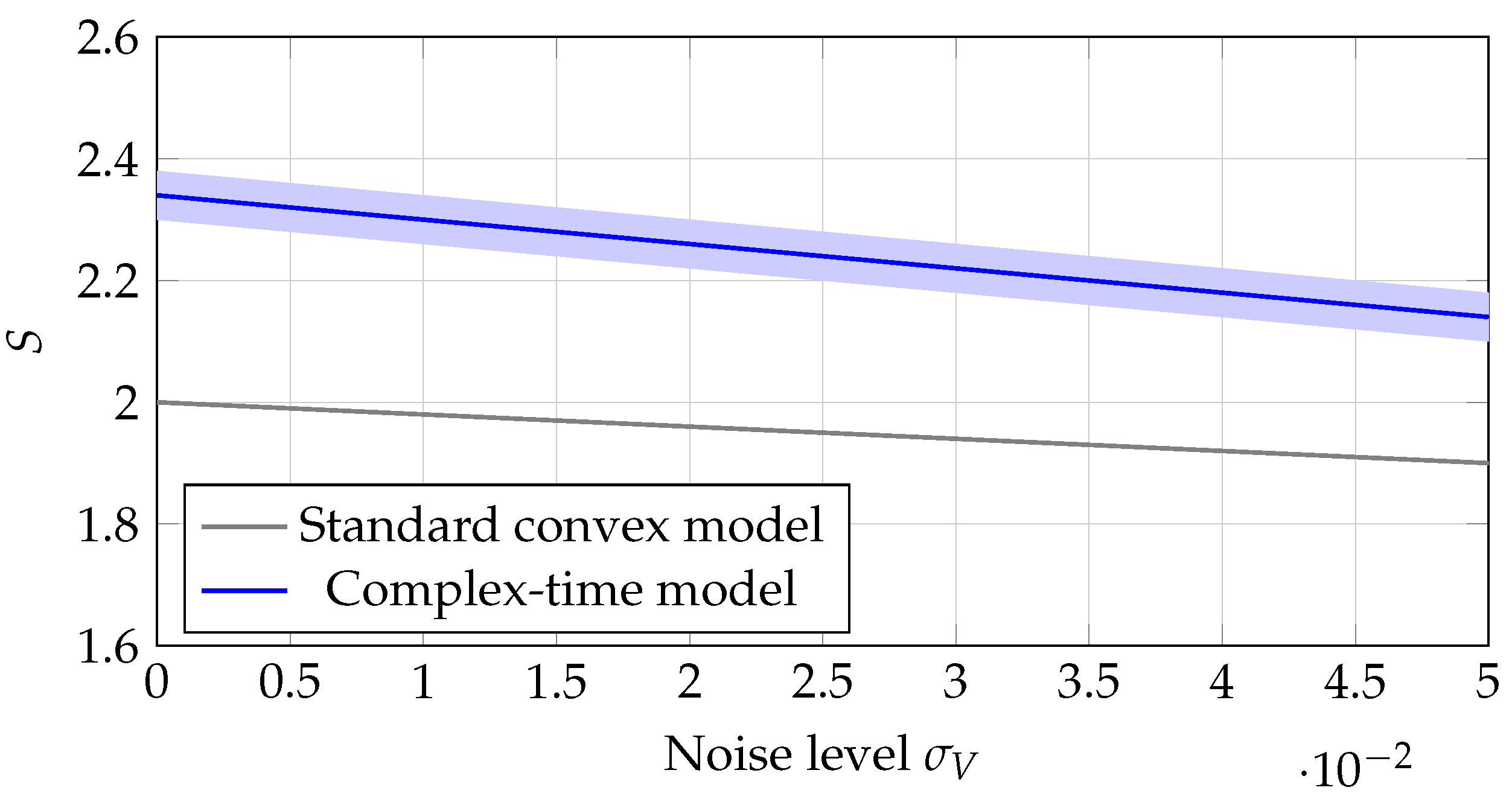

Table 1.
Comparison of several decoherence models under the temporal CHSH protocol.
| Model | Visibility form | Convexity | CHSH bound |
|---|---|---|---|
| Standard environmental decoherence | Yes | ||
| One-dimensional stochastic model | Yes | ||
| Gaussian classical noise | Yes | ||
| Complex-time model | No (nonlinear in ) | possible |
Table 2.
Visibility as a function of the dimensionless parameter .
| 0.0 | 1.00 |
| 0.3 | 0.74 |
| 0.6 | 0.55 |
| 1.2 | 0.30 |
| 1.8 | 0.17 |
| 2.4 | 0.09 |
Table 3.
Imaginary-time difference as a function of the rotation angle .
| (rad) | (fs) | |
|---|---|---|
| 0.0 | 0.00 | 0.0 |
| 0.2 | 0.20 | 10.0 |
| 0.4 | 0.39 | 19.5 |
| 0.6 | 0.56 | 28.0 |
| 0.8 | 0.72 | 36.0 |
| 1.0 | 0.84 | 42.0 |
Table 4.
Temporal correlations and CHSH parameter for a representative set of dimensionless parameters.
Table 4.
Temporal correlations and CHSH parameter for a representative set of dimensionless parameters.
| Setting | |||
|---|---|---|---|
| 0.0 | 1.00 | 1.00 | |
| 0.5 | 0.61 | 0.22 | |
| 0.5 | 0.61 | 0.22 | |
| 3.0 | 0.05 | -0.90 |
Table 5.
Illustrative internal-time evolution under the phenomenological relaxation law .
| t (ps) | |
|---|---|
| 0 | 0.000 |
| 1 | -0.048 |
| 2 | -0.096 |
| 3 | -0.144 |
| 4 | -0.192 |
Table 6.
Effect of a late choice on visibility.
| Configuration | (fs) | ||
|---|---|---|---|
| Closed | 0.0 | 0 | 1.00 |
| Open | 0.6 | 28 | 0.55 |
Disclaimer/Publisher’s Note: The statements, opinions and data contained in all publications are solely those of the individual author(s) and contributor(s) and not of MDPI and/or the editor(s). MDPI and/or the editor(s) disclaim responsibility for any injury to people or property resulting from any ideas, methods, instructions or products referred to in the content. |
© 2026 by the authors. Licensee MDPI, Basel, Switzerland. This article is an open access article distributed under the terms and conditions of the Creative Commons Attribution (CC BY) license (http://creativecommons.org/licenses/by/4.0/).
Copyright: This open access article is published under a Creative Commons CC BY 4.0 license, which permit the free download, distribution, and reuse, provided that the author and preprint are cited in any reuse.