Submitted:
22 February 2026
Posted:
26 February 2026
You are already at the latest version
Abstract
One of the main tools in Statistical Process Control (SPC) for monitoring quality is the control chart. Simultaneous multivariate control charts are widely used to monitor shifts in the process mean and variability at the same time. One Shewhart-type simul-taneous multivariate chart is the Max-Half-Mchart, which can detect both small and large shifts in the mean and variability. However, outliers can distort the estimation of process parameters used to set control limits. In addition, outliers can cause two related problems, namely the masking effect and the swamping effect. Recent studies have highlighted the importance of cellwise outliers. Previous studies have shown that cellwise contamination can trigger outlier propagation. Therefore, casewise-based ro-bust estimators become less relevant under such conditions. CellMCD is a robust method for estimating location and covariance by integrating cellwise outlier detection into a single objective function. This study aims to develop a robust Max-Half-M chart based on cellMCD. Based on simulation studies under different correlation levels and contamination proportions, the proposed chart shows more stable performance than the conventional chart and the robust Fast-MCD–based version, as indicated by higher AUC values and lower FN rates. The ARL analysis also suggests that the cellMCD-based chart tends to detect small to moderate shifts faster. In the real-data application, the cellMCD-based chart successfully detects seven out-of-control signals, which is more than the comparison charts.
Keywords:
simultaneous multivariate control charts
; Max-Half-Mchart
; cellwise contamination
; cellMCD
1. Introduction
Statistical Process Control (SPC) is an important approach to monitor product quality and keep a production process consistent. SPC monitors the process mean and variability across several quality characteristics, so process problems can be detected early before products go beyond specification limits [1]. One of the main SPC tools is the control chart, introduced by Walter A. Shewhart in 1924 to distinguish common cause variation from special cause variation in a process [2]. Based on the number of quality characteristics, control charts are classified into univariate and multivariate charts. Univariate charts monitor one characteristic at a time, while multivariate control charts monitor two or more correlated characteristics at the same time.
A wide range of multivariate control charts has been developed in the literature. Hotelling’s chart extends the -test and the chart to detect shifts in the process mean vector [3]. To better detect small mean shifts, MCUSUM and MEWMA charts have been proposed [4,5]. For monitoring changes in multivariate variability, the generalized variance chart uses the determinant of the sample covariance matrix [1]. For individual observations, a successive difference approach has also been introduced [6]. Other variability measures include IGV, vector variance, and methods that combine generalized variance with the trace of the covariance matrix [7,8,9]. In addition, some charts focus on changes in the correlation structure [10], and the chart has been proposed for subgroup data [11].
Simultaneous control charts have also been developed to monitor the process mean and variability at the same time. A Shewhart type simultaneous chart was first introduced using a modified boxplot for subgroup data [12]. Later, the Max Chart was proposed by combining the chart and the chart [13]. For the bivariate case, a Max-Chart based on Hotelling’s statistic and the generalized variance was developed for subgroup data [14]. This idea was then extended to the multivariate setting and became known as the Max-Mchart [15]. Further work includes the Max-Mchart Chart with a gamma distribution transformation [16]. In addition, the Max-Mchart and the Max Half-Mchart have been developed for individual observations using standard normal and half normal transformations, and they have also been studied for subgroup data [17,18].
However, conventional control charts are known to be sensitive to outliers. Outliers can affect the estimation of process parameters used to set control limits, which may result in wider or stretched control limits [19]. A key weakness of classical estimators is their vulnerability to masking and swamping effects. Masking refers to a loss of detection power when the true number of outliers is larger than assumed, so extreme outliers may not be detected, leading to false negatives [20]. In contrast, swamping occurs when normal observations are incorrectly flagged as outliers, leading to false positives [21].
Several studies have been developed to address the problem of casewise outliers. Robust estimators such as the Minimum Volume Ellipsoid (MVE) and the Minimum Covariance Determinant (MCD) were introduced as outlier resistant estimators of location and covariance. MVE searches for the minimum volume ellipsoid covering at least observations, while MCD selects an -subset with the smallest covariance determinant [22]. To reduce computational cost, the Fast MCD algorithm was proposed [23]. The efficiency of MCD was later improved by reweighting, leading to RMCD [24], and a deterministic version was introduced as Det MCD [25]. For fat or high dimensional data, the Minimum Regularized Covariance Determinant (MRCD) was proposed to stabilize robust covariance estimation [26]. MRCD was further extended through a kernel approach, known as Kernel MRCD, to provide more flexibility for non-elliptical data [27].
More recently, attention has shifted to cellwise outliers [28]. Cellwise contamination may cause outlier propagation: even if only a small fraction of cells is contaminated, many rows can become contaminated because a single outlying cell is enough to affect an entire observation. The expected proportion of contaminated rows is , where is the fraction of contaminated cells and is the number of variables [28]. In high dimensional settings, a small can therefore lead to a large fraction of contaminated rows, which may reduce the accuracy of casewise robust methods. A widely used method for cellwise detection is Detecting Deviating Data Cells (DDC), which predicts each cell and flags cells that deviate strongly from their predictions [29]. Several approaches have also been proposed to obtain covariance estimators that are robust under cellwise contamination, for example using rank-based correlations, robust pairwise correlations, or wrapping transformations to produce a positive semidefinite covariance matrix [30,31,33]. However, these methods follow a two steps strategy, where outlier detection is separated from parameter estimation. To overcome this limitation, the cellMCD estimator was introduced to jointly estimate location and covariance while detecting cellwise outliers, using an observed likelihood framework for incomplete data and a penalty term that limits the number of flagged cells [34]. This estimator is robust under cellwise contamination, efficient for clean data, and implemented with C steps to ensure improvement of the objective function at each iteration.
Based on these considerations, this study proposes a simultaneous control chart, namely Max Half-Mchart based on cellMCD estimators, which is robust to cellwise outlier contamination. To demonstrate the suitability of the proposed chart, its performance is compared with the conventional Max Half-Mchart and the Max Half-Mchart based on Fast-MCD estimators. The remainder of this paper is organized as follows. Section 2 introduces the proposed cellMCD based-Max Half-Mchart. Section 3 describes the methodology and implementation procedures. Section 4 evaluates the chart performance in detecting outliers and process shifts. Section 5 presents applications to simulated and real data. Finally, Section 6 provides conclusions and directions for future research.
2. Materials and Methods
2.1. Max-Half-Mchart
The Max-Mchart is known to have limitations in providing accurate results due to its use of transformations based on the standard normal distribution. This limitation motivates an alternative approach to avoid negative-domain issues when computing quantiles. One proposed solution is to use the half-normal distribution, which has a positive support from to . This idea forms the basis for developing the Max-Half-Mchart.
The Max-Half-Mchart is constructed using the same combined framework as the The Max-Mchart, namely Hotelling’s and the successive difference approach. The simultaneous statistics for monitoring the process mean and variability in the Max-Half-Mchart for individual observations are defined as follows [17]:
and
where denotes the cumulative distribution function of the standard half normal distribution and denotes the cumulative distribution function of the chi square distribution with degrees of freedom. Because the half normal transformation produces statistics on a positive support, the absolute value is no longer required. The Max Half M chart statistic is then defined by
𝑍𝑖𝐼𝐻=Q−1𝐻𝑝𝐱𝑖−𝛍0′𝚺0−1𝒙𝑖−𝛍0,
The Max Half M chart uses only an upper control limit, since . Because the distribution of is not available in closed form and is typically skewed. The upper control limit is estimated using a nonparametric procedure such as bootstrap approach [17].
2.2. Cellwise Minimum Covariance Determinant (CellMCD)
The Minimum Covariance Determinant (MCD) estimator is theoretically defined by selecting an -subset of observations that minimizes the determinant of the covariance matrix. MCD is a robust estimator designed mainly for casewise outliers, where entire rows are atypical. However, in several practical applications, contamination is cellwise. Only some entries in a row are outlying, while the remaining cells still contain valid information. Under dominant cellwise contamination, discarding whole rows may remove useful information and reduce efficiency. To address this issue, cellMCD was developed as a cellwise extension of MCD [34].
CellMCD introduces a binary weight matrix , where if cell is kept as clean and if the cell is flagged as an outlier or missing value. The notation , , , and follows the observed likelihood framework for incomplete data [35]. The squared distance term is defined as the partial Mahalanobis distance computed on the observed cells [36]. The matrix is not specified in advance but is estimated jointly with the model parameters. The trimming level is applied to the number of unflagged cells per column rather than to the number of unflagged cases. The cellMCD objective function is defined as follows [34].
under the constrains The penalty parameter is computed as
where denotes the -quantile of the chi-square distribution with one degree of freedom. The term is the conditional variance of variable based on the initial covariance estimate , defined by . The value is recommended because it leads to more efficient estimates [34].
In the first stage, the data are robustly standardized columnwise using (Rousseeuw). Next, initial estimates are obtained using the DDCW estimator [37]. The algorithm then applies the C-step (Part A), which updates the weight matrix at iteration while keeping and fixed. For each cell, the update is based on the change in the objective function when setting versus , defined by
where and are the conditional mean and conditional variance given the currently unflagged (observed) cells in row (indexed by ). If holds for at least indices in column , the objective is minimized by setting for those cells and for the remaining cells. Otherwise, the minimum is attained by setting for the observations with the smallest values and for the others. After cycling through all columns, the updated weight matrix is obtained.
After obtaining from the C-step (Part A), the C-step (Part B) updates and using an EM-type framework for incomplete data, where flagged cells are treated as missing. For each observation , the index set of retained (observed) cells is defined as and with and . The data vector , mean , and covariance matrix are partitioned into observed and missing blocks, which allows structured imputation and parameter updating.
In the E-step, for rows with missing cells , the missing block is imputed by the conditional mean given the observed block,
and the corresponding conditional covariance is computed to correct for the variance contribution of imputation,
These quantities define the imputed matrix , where for observed cells and for flagged cells.
In the M-step, the mean estimator is updated as the average of the imputed observations,
and the covariance estimator is obtained from the sample covariance of plus a bias-correction matrix . The matrix aggregates the contributions of on the missing blocks for each row and is averaged across all observations. The updated covariance is therefore
To keep the covariance matrix well-conditioned, the constraint is enforced with by truncating small eigenvalues, and the resulting matrix is denoted by . The C-step (Parts A and B) is repeated until convergence. After convergence at iteration , the standardized-scale estimates are and . The estimates on the original scale are obtained by back-transformation as
where .
2.3. CellMCD Based-Max Half-Mchart
This study adapts the Max Half M chart by substituting the classical estimators of the mean vector and covariance matrix in Equations (10) and (11) with robust estimates of location and scatter. The replacements are obtained from the cellMCD estimator, which is designed to reduce the influence of cellwise contamination. As a result, the control statistics become more reliable under outliers. The statistics for monitoring the process mean vector and variability for individual observations based on cellMCD are defined as follows:
and
Then, the cellMCD-based Max Half M chart statistic is constructed by combining the mean and variability components into a single monitoring statistic. The cellMCD-based Max Half M chart statistic is given by:
Estimating the upper control limit (UCL) for the Max-Half-Mchart is carried out using a resampling strategy based on bootstrap methods [17]. In practice, calibrating the chart to achieve a target in-control average run length (ARL) is computationally demanding. For this reason, Monte Carlo simulation is used to approximate the in-control behavior of the chart and to link candidate UCL values to the resulting ARL [38]. In this study, the UCL is therefore determined through a combined bootstrap–Monte Carlo procedure, which is described in Algorithm 2.
3. Methodology
This section presents the methodological framework used in this study. The proposed cellMCD-based Max-Half-Mchart is implemented in two main stages. First, the cellMCD-based Max-Half-Mchart statistics are computed. Second, the upper control limit is estimated by combining a bootstrap resampling scheme with Monte Carlo simulation. the procedure for computing the charting statistics and plotting the control chart is described as follows:
| Algorithm 1 Procedure to Compute and Plot the Proposed cellMCD-Based Max-Half-M Chart |
| Step 1. Set . Step 2. Compute the robust mean vector and robust covariance matrix using equations (10) and (11). Step 3. Calculate the mean statistic and the variability statistic using equations (12) and (13). Then form the simultaneous statistic using equation (14). Step 4. Estimate the upper control limit for the proposed based on the bootstrap and Monte Carlo simulation using Algorithm 2. Step 5. Plot against .
|
After computing the cellMCD-based Max Half M chart statistics, the next step is to determine the upper control limit (UCL) using Algorithm 2 as follows:
| Algorithm 2 Bootstrap and Monte Carlo Control Limit |
| Step 1. Set . Step 2. Obtain the robust estimates and using equations (10) and (11). Step 3. For , repeat: a. Generate observations from the multivariate normal distribution b. Compute the cellMCD-based Max-Half-Mchart statistic for using the simulated sample. c. Apply bootstrap resampling (with replacement) to obtain 1000 bootstrap values of . d. For replication , compute the empirical th percentile of the 1000 bootstrap values, denoted by Step 4. Estimate the UCL by averaging these percentile values across the 1000 Monte Carlo replications: |
The performance evaluation of the control chart includes ARL under process shifts and a confusion matrix assessment for outlier detection. The effectiveness of the classification is assessed through measures of correct decisions and classification errors. In this setting, correct decisions can be divided into two categories:

Table 1.
Confusion Matrix Table.
| Actual | Detection | |
|---|---|---|
| Outlier | Normal | |
| Outlier | True Positives (TP) | False Negatives (FN) |
| Normal | False Positives (FP) | True Negatives (TN) |
True positives (TP) refer to outlier observations that are correctly identified as outliers. True negatives (TN) refer to normal observations that are correctly identified as normal. Misclassification errors are also grouped into two types. False positives (FP) occur when a normal observation is incorrectly flagged as an outlier, which leads to a false alarm. False negatives (FN) occur when an outlier observation is missed and incorrectly classified as normal, which results in an undetected outlier. These errors are summarized using the false positive rate (FP Rate) and false negative rate (FN Rate) [39].
In addition, the overall detection ability is measured using the area under the curve (AUC) defined as [40]:
4. Result
4.1. Simulation Study
In this section, the performance of the robust Max-Half-Mchart is evaluated through a simulation study to assess its ability to detect outliers. The simulation begins by generating multivariate normal data , where the mean vector is of dimension . The variance of each quality characteristic is set to 1, and an exchangeable correlation structure is assumed across characteristics. Therefore, the covariance matrix is defined as with .
Next, cellwise contamination is introduced by replacing a fraction of cells with contaminated values. For each column of the data matrix, cell indices are randomly selected for contamination, and the selected cells are then replaced by contaminated values controlled by the parameter . A larger indicates more severe deviations in the contaminated cells. In this study, is used. This contamination mechanism is implemented using the generateData function from the R package cellWise [41]. The outlier proportion is varied across four scenarios: 5%, 10%, 15%, and 20%. The proportion of cellwise outlier contamination is limited to 20% because it remains below the theoretical breakdown point of the cellMCD estimator, which is approximately 25% under the default choice , given by [34]. The number of quality characteristics is set to .
For performance evaluation, each observation that contains at least one contaminated cell is treated as a contaminated observation and assigned label 1; otherwise, it is assigned label 0. Furthermore, because the Max-Half statistic is computed based on successive difference , a pair label is defined for each pair. The pair is assigned label 1 if at least one of the two observations in is contaminated, and label 0 if both are normal. The proposed robust Max-Half-Mchart based on cellMCD is compared with the conventional chart and the robust Max-Half-Mchart based on Fast-MCD. The chart performance is considered satisfactory when it achieves high Accuracy and AUC, along with low false positive rate (FP rate) and false negative rate (FN rate).
Outlier detection using the conventional control chart was evaluated first, and the detailed performance results are reported in Table 2. Table 2 summarizes the Accuracy, AUC, false positive rate (FP rate), and false negative rate (FN rate) of the conventional Max-Half-Mchart chart under different correlation levels and outlier proportions. The results indicate that the conventional Max-Half-Mchart performs poorly for cellwise contamination. The FN rate is extremely high, ranging from 0.8579 to 0.9999, meaning that most truly contaminated observations are not detected. Consistently, the AUC values remain close to 0.5, suggesting that the chart has almost no discriminatory power beyond random guessing. Regarding the effect of correlation, increasing from 0.3 to 0.7 does not lead to a meaningful improvement. Although a slight increase in AUC is observed at 5% outliers when is higher, the overall performance of the chart remains unsatisfactory.
Table 3 shows the simulation results of the Fast-MCD–based Max-Half-M chart under different correlation levels and outlier proportions. Overall, this method performs much better than the conventional chart, as indicated by high Accuracy and AUC values and very small false positive rates (FP rates) in almost all scenarios. Under low contamination, the Fast-MCD approach shows good performance. For example, when , the Accuracy reaches approximately 0.9882 with an AUC of 0.9904, while the false negative rate (FN rate) remains relatively low. A similar pattern is also observed for . These results suggest that when the correlation among variables is sufficiently strong, the robust Fast-MCD estimator can maintain high sensitivity for outlier detection.
As the outlier proportion increases, the performance decreases, particularly under weaker correlation. For , increasing the outlier percentage from 10% to 20% reduces the Accuracy from 0.8262 to 0.2131 and sharply increases the FN rate from 0.2660 to 0.8816. The AUC also drops to 0.5592, indicating much weaker discrimination under heavy contamination and low correlation. Overall, these findings confirm that the Fast-MCD–based Max-Half-Mchart becomes less effective when cellwise contamination is severe.
Table 4 presents the simulation results of the cellMCD-based Max-Half-M chart under different correlation levels and outlier proportions. Overall, the method shows stable and strong performance across all scenarios, characterized by high Accuracy and AUC values, very small false positive rates (FP rates), and false negative rates (FN rates) that tend to decrease as the outlier proportion increases. For , the performance of the cellMCD approach does not deteriorate when contamination becomes more severe. When the outlier proportion increases from 5% to 20%, the Accuracy remains high, while the FN rate decreases from 0.2279 to 0.1167 and the AUC increases from 0.8851 to 0.9413. This pattern indicates that cellMCD can maintain consistent outlier detection ability even under low-correlation conditions.
A similar trend is observed for . As the contamination level increases from 5% to 20%, the FN rate decreases from 0.1231 to 0.0671, the AUC increases from 0.9375 to 0.9660, and the Accuracy stays at a high level. For , the performance becomes very strong. Accuracy consistently exceeds 0.98, AUC ranges from 0.9861 to 0.9918, and the FN rate remains very small. Across all values of , the FP rate also stays low. In summary, Table 4 confirms that the cellMCD-based Max-Half-M chart is more robust and more reliable for cellwise contamination, both under low and high correlation, while maintaining a low false alarm rate even when the outlier proportion increases.
To make the performance comparison among charts clearer, radar charts are provided in Figure 1, Figure 2 and Figure 3. These figures present the comparison of Accuracy, FN rate, and AUC under three correlation settings: (a) , (b) , and (c) , with outlier proportions of 5%, 10%, 15%, and 20%. The FP rate is not visualized because its differences across charts are very small and thus do not provide additional insight.
Figure 1 shows that the cellMCD-based Max-Half-Mchart generally forms the largest area across most scenarios, indicating the highest and most stable Accuracy as the outlier proportion increases. Figure 2 provides a more comprehensive view of outlier detection ability. The cellMCD-based Max-Half-Mchart produces the smallest area in all panels, reflecting the lowest FN rates. In contrast, the Fast-MCD–based Max-Half-Mchart lies in between: it performs better than the conventional chart, but under higher contamination levels it still exhibits relatively larger FN rates in several cases.
Figure 3 shows a pattern consistent with the previous metrics. The cellMCD-based Max-Half-Mchart achieves the highest and most stable AUC values across all combinations of and outlier proportions, indicating strong discrimination between normal and contaminated observations. The Fast-MCD–based Max-Half-Mchart performs well under low to moderate contamination, but its performance tends to decrease when the outlier proportion increases, particularly under low correlation. Conversely, the conventional chart consistently shows the lowest AUC values, suggesting weak separation capability under cellwise contamination.
Figure 1 shows that the cellMCD-based Max-Half-M chart generally forms the largest area across most scenarios, indicating the highest and most stable Accuracy as the outlier proportion increases. Figure 2 provides a more comprehensive view of outlier detection ability. The cellMCD-based Max-Half-M chart produces the smallest area in all panels, reflecting the lowest FN rates. In contrast, the Fast-MCD–based Max-Half-M chart lies in between: it performs better than the conventional chart, but under higher contamination levels it still exhibits relatively larger FN rates in several cases.
Figure 3 (AUC) shows a pattern consistent with the previous metrics. The cellMCD-based Max-Half-M chart achieves the highest and most stable AUC values across all combinations of and outlier proportions, indicating strong discrimination between normal and contaminated observations. The Fast-MCD–based Max-Half-M chart performs well under low to moderate contamination, but its performance tends to decrease when the outlier proportion increases, particularly under low correlation. Conversely, the conventional chart consistently shows the lowest AUC values, suggesting weak separation capability under cellwise contamination.
To clarify how each chart produces signals on the simulated data, Figure 4, Figure 5 and Figure 6 present the Max-Half-M statistics plots under three contamination levels, namely 5%, 15%, and 20%. Visually, the cellMCD-based Max-Half-M chart provides the clearest separation between normal observations and outliers. Contaminated observations more frequently exceed the UCL, whereas normal observations tend to remain below the UCL. This pattern is consistent across all contamination levels, even when the outlier proportion increases to 20%.
In contrast, the conventional chart and the Fast-MCD–based Max-Half-M chart still show many contaminated observations falling below the UCL, especially under higher contamination, indicating a higher false negative rate. Therefore, Figure 4, Figure 5 and Figure 6 support the results reported in the previous tables and confirm that the cellMCD-based Max-Half-M chart is the most reliable approach for detecting cellwise contamination, as it maintains high detection sensitivity without excessively increasing false alarms.
4.2. Detecting Shift
In statistical process control performance evaluation, one of the fundamental metrics is the Average Run Length (ARL). ARL is widely used to assess the efficiency of a control chart because it reflects how quickly the chart can detect a process change (shift). The ARL is defined as the average number of observations required until the control chart signals an out-of-control condition for the first time. A control chart is considered desirable when it has a large under in-control conditions, indicating a low false alarm rate. Conversely, a smaller indicates faster detection of real process changes. Therefore, the smaller the value that is close to 1 indicates that the chart can detect process shifts more effectively [1].
In this study, ARL values were estimated using a simulation procedure. The simulations considered several shift scenarios, including shifts in the process mean, shifts in the covariance matrix, and simultaneous shifts in both. Experiments were conducted for a quality-characteristic dimension of and three correlation settings . Under these settings, the performance of each chart can be compared objectively and comprehensively based on its ability to detect process shifts. For comparison purposes, the ARL values of the conventional and Fast-MCD–based charts were adopted from the preprint study by [42] and treated as benchmark results.
Table 5.
ARL of the Conventional Max-Half-MChart for and .
| a | b | ||||||||||||
|---|---|---|---|---|---|---|---|---|---|---|---|---|---|
| 1 | 1.25 | 1.5 | 1.75 | 2 | 2.25 | 2.5 | 2.75 | 3 | 3.25 | 3.5 | 3.75 | 4 | |
| 0 | 372.94 | 80.06 | 28.39 | 14.18 | 8.91 | 6.00 | 4.67 | 3.37 | 2.95 | 2.54 | 2.22 | 2.00 | 1.85 |
| 0.25 | 310.41 | 72.76 | 26.31 | 13.54 | 8.58 | 5.78 | 4.60 | 3.66 | 2.85 | 2.53 | 2.20 | 2.00 | 1.85 |
| 0.5 | 215.25 | 52.65 | 22.32 | 12.56 | 7.71 | 5.41 | 4.12 | 3.30 | 2.77 | 2.50 | 2.13 | 1.98 | 1.75 |
| 0.75 | 122.80 | 39.15 | 17.88 | 10.65 | 6.81 | 4.88 | 3.61 | 3.06 | 2.57 | 2.23 | 2.13 | 1.89 | 1.71 |
| 1 | 63.71 | 25.38 | 12.36 | 8.14 | 5.21 | 4.37 | 3.46 | 2.95 | 2.47 | 2.18 | 1.99 | 1.77 | 1.64 |
| 1.25 | 31.20 | 14.70 | 8.63 | 6.25 | 4.37 | 3.48 | 3.04 | 2.63 | 2.29 | 1.97 | 1.85 | 1.68 | 1.60 |
| 1.5 | 16.26 | 8.80 | 6.37 | 4.23 | 3.53 | 3.02 | 2.51 | 2.20 | 1.94 | 1.81 | 1.71 | 1.59 | 1.48 |
| 1.75 | 8.44 | 5.37 | 4.35 | 3.26 | 2.93 | 2.50 | 2.21 | 1.97 | 1.79 | 1.69 | 1.56 | 1.47 | 1.46 |
| 2 | 5.26 | 3.91 | 3.18 | 2.66 | 2.30 | 2.12 | 1.95 | 1.85 | 1.63 | 1.51 | 1.43 | 1.43 | 1.38 |
| 2.25 | 3.37 | 2.73 | 2.35 | 2.11 | 1.92 | 1.75 | 1.67 | 1.51 | 1.50 | 1.43 | 1.37 | 1.33 | 1.25 |
| 2.5 | 2.41 | 2.07 | 1.92 | 1.73 | 1.62 | 1.63 | 1.52 | 1.45 | 1.36 | 1.39 | 1.33 | 1.24 | 1.24 |
| 2.75 | 1.72 | 1.72 | 1.54 | 1.48 | 1.47 | 1.34 | 1.35 | 1.28 | 1.32 | 1.25 | 1.21 | 1.20 | 1.19 |
| 3 | 1.42 | 1.34 | 1.33 | 1.28 | 1.30 | 1.30 | 1.24 | 1.24 | 1.19 | 1.17 | 1.16 | 1.15 | 1.13 |
Table 6.
ARL of the Fast-MCD-Based Max-Half-MChart for and .
| a | b | ||||||||||||
|---|---|---|---|---|---|---|---|---|---|---|---|---|---|
| 1 | 1.25 | 1.5 | 1.75 | 2 | 2.25 | 2.5 | 2.75 | 3 | 3.25 | 3.5 | 3.75 | 4 | |
| 0 | 371.13 | 80.56 | 29.22 | 14.51 | 9.41 | 6.22 | 4.63 | 3.84 | 3.02 | 2.57 | 2.25 | 2.17 | 1.88 |
| 0.25 | 326.69 | 70.36 | 28.05 | 13.81 | 8.47 | 5.83 | 4.53 | 3.53 | 2.92 | 2.50 | 2.24 | 1.97 | 1.88 |
| 0.5 | 222.40 | 59.14 | 23.22 | 12.57 | 7.86 | 5.30 | 4.01 | 3.28 | 2.82 | 2.43 | 2.23 | 1.96 | 1.85 |
| 0.75 | 129.17 | 39.18 | 18.81 | 10.13 | 6.78 | 4.84 | 4.00 | 3.17 | 2.61 | 2.32 | 2.16 | 1.88 | 1.78 |
| 1 | 65.58 | 23.70 | 12.51 | 8.22 | 5.65 | 4.39 | 3.38 | 2.81 | 2.54 | 2.25 | 2.00 | 1.80 | 1.71 |
| 1.25 | 31.82 | 15.46 | 9.08 | 6.34 | 4.69 | 3.55 | 2.99 | 2.47 | 2.23 | 2.05 | 1.81 | 1.77 | 1.64 |
| 1.5 | 16.50 | 9.28 | 6.15 | 4.76 | 3.64 | 3.03 | 2.49 | 2.30 | 2.10 | 1.87 | 1.68 | 1.61 | 1.56 |
| 1.75 | 8.97 | 5.83 | 4.30 | 3.39 | 3.01 | 2.34 | 2.24 | 1.88 | 1.80 | 1.66 | 1.57 | 1.48 | 1.46 |
| 2 | 5.08 | 3.78 | 3.19 | 2.66 | 2.36 | 2.08 | 1.96 | 1.79 | 1.63 | 1.57 | 1.51 | 1.43 | 1.37 |
| 2.25 | 3.33 | 2.66 | 2.53 | 2.19 | 1.95 | 1.81 | 1.69 | 1.56 | 1.47 | 1.41 | 1.38 | 1.34 | 1.31 |
| 2.5 | 2.37 | 2.04 | 1.90 | 1.78 | 1.70 | 1.53 | 1.50 | 1.44 | 1.36 | 1.32 | 1.27 | 1.31 | 1.23 |
| 2.75 | 1.72 | 1.71 | 1.59 | 1.50 | 1.49 | 1.44 | 1.36 | 1.36 | 1.27 | 1.24 | 1.22 | 1.21 | 1.19 |
| 3 | 1.44 | 1.43 | 1.37 | 1.31 | 1.35 | 1.30 | 1.30 | 1.22 | 1.19 | 1.18 | 1.16 | 1.14 | 1.16 |
Table 1 shows the ARL values of the conventional Max-Half-Mchart for . When the mean vector shifts from to while the covariance matrix remains in control (), the ARL of the conventional Max-Half-Mchart decreases from 373 to 310. The ARL further decreases from 372 to 80 when the covariance matrix is inflated by a factor of 1.5 () while the mean vector remains in control ().
From Table 2, the ARL of the robust Fast-MCD–based Max-Half-Mchart decreases from 371 to 326 under the same mean shift to with . It also decreases from 371 to 80 when the covariance matrix is inflated by a factor of 1.5 () while the mean remains in control. Table 3 shows that the robust cellMCD-based Max-Half-M chart achieves a faster response, with the ARL decreasing from 371 to 263 under the mean shift and from 371 to 62 when the covariance matrix is inflated by a factor of 1.5 () with the mean still in control. These results indicate that the cellMCD-based robust Max-Half-Mchart detects both mean shifts and covariance changes more quickly than the other charts. A similar conclusion is observed for larger shifts, where the cellMCD-based chart also provides the fastest detection for changes in both the mean and the covariance structure.
Table 7, Table 8 and Table 9 report the ARL values of the three charts for . Under small shifts, the robust cellMCD-based Max-Half-Mchart detects both mean shifts and covariance changes faster than the other charts. However, under large shifts, the conventional chart provides faster detection for both mean shifts and covariance shifts. To make the comparison clearer, Figure 7 presents a graphical visualization of the detection performance of the three charts at for mean shifts, covariance shifts, and simultaneous shifts in both.
Figure 7a compares the ARL values when a shift occurs in the mean vector (parameter ) while the covariance matrix remains in control (). Figure 7b shows the ARL comparison when the mean vector stays in control () and a shift occurs in the covariance matrix, represented by the inflation factor . Figure 7c presents the ARL comparison when shifts occur simultaneously in both the mean vector and the covariance matrix. In general, increasing the correlation among variables has the most noticeable effect in the mean-shift case. The ARL tends to be larger at higher for small to moderate shifts, which means mean shifts are detected more slowly when the dependence among variables becomes stronger. However, when the mean shift becomes larger, all ARL curves quickly approach one, so the differences across correlation levels become much smaller. In contrast, in Figure 7b,c, the ARL curves for different values are close to each other, indicating that correlation has only a minor effect when the covariance shifts or when both mean and covariance shift. In these cases, the ARL drops sharply as soon as or the shift level increases, showing fast detection. Therefore, correlation mainly affects the sensitivity of the charts for detecting small mean shifts, while for covariance shifts and simultaneous shifts, changes in correlation do not substantially change the detection speed.
Table 8.
ARL of the Conventional Max-Half-MChart for and .
| a | b | ||||||||||||
|---|---|---|---|---|---|---|---|---|---|---|---|---|---|
| 1 | 1.25 | 1.5 | 1.75 | 2 | 2.25 | 2.5 | 2.75 | 3 | 3.25 | 3.5 | 3.75 | 4 | |
| 0 | 372.44 | 77.84 | 28.33 | 14.09 | 8.70 | 5.85 | 4.56 | 3.48 | 2.93 | 2.59 | 2.30 | 2.00 | 1.87 |
| 0.25 | 308.73 | 71.61 | 26.26 | 14.57 | 9.26 | 6.15 | 4.32 | 3.52 | 2.92 | 2.48 | 2.20 | 1.98 | 1.87 |
| 0.5 | 251.44 | 63.97 | 24.55 | 13.34 | 7.82 | 5.84 | 4.27 | 3.53 | 2.92 | 2.47 | 2.18 | 1.95 | 1.87 |
| 0.75 | 194.19 | 51.68 | 21.28 | 11.60 | 7.64 | 5.18 | 4.22 | 3.40 | 2.83 | 2.37 | 2.10 | 1.94 | 1.80 |
| 1 | 126.91 | 37.13 | 17.74 | 9.83 | 6.47 | 4.70 | 3.81 | 3.09 | 2.75 | 2.23 | 2.10 | 1.92 | 1.79 |
| 1.25 | 72.12 | 27.71 | 13.50 | 7.89 | 5.46 | 4.52 | 3.64 | 2.88 | 2.53 | 2.16 | 1.94 | 1.75 | 1.63 |
| 1.5 | 40.55 | 18.17 | 10.45 | 6.68 | 5.18 | 3.79 | 3.16 | 2.61 | 2.32 | 2.04 | 1.87 | 1.79 | 1.64 |
| 1.75 | 25.97 | 11.60 | 7.67 | 5.51 | 4.27 | 3.32 | 2.83 | 2.57 | 2.12 | 1.92 | 1.76 | 1.59 | 1.51 |
| 2 | 14.65 | 8.97 | 5.80 | 4.17 | 3.36 | 2.91 | 2.56 | 2.30 | 1.99 | 1.83 | 1.70 | 1.55 | 1.50 |
| 2.25 | 9.48 | 5.83 | 4.48 | 3.57 | 2.86 | 2.46 | 2.28 | 2.00 | 1.86 | 1.72 | 1.61 | 1.45 | 1.39 |
| 2.5 | 6.20 | 4.30 | 3.46 | 2.95 | 2.52 | 2.22 | 2.07 | 1.84 | 1.66 | 1.57 | 1.53 | 1.42 | 1.38 |
| 2.75 | 4.23 | 3.37 | 2.78 | 2.42 | 2.10 | 1.90 | 1.79 | 1.69 | 1.58 | 1.49 | 1.46 | 1.41 | 1.35 |
| 3 | 3.27 | 2.48 | 2.31 | 2.04 | 1.89 | 1.75 | 1.67 | 1.53 | 1.49 | 1.40 | 1.32 | 1.31 | 1.27 |
Table 9.
ARL of the Fast-MCD-Based Max-Half-MChart for and .
| a | b | ||||||||||||
|---|---|---|---|---|---|---|---|---|---|---|---|---|---|
| 1 | 1.25 | 1.5 | 1.75 | 2 | 2.25 | 2.5 | 2.75 | 3 | 3.25 | 3.5 | 3.75 | 4 | |
| 0 | 370.54 | 77.70 | 29.56 | 14.84 | 9.36 | 6.13 | 4.53 | 3.72 | 3.09 | 2.51 | 2.31 | 1.98 | 1.87 |
| 0.25 | 337.26 | 75.36 | 29.64 | 14.69 | 9.26 | 6.27 | 4.42 | 3.64 | 2.96 | 2.50 | 2.16 | 1.97 | 1.87 |
| 0.5 | 273.39 | 69.17 | 26.64 | 12.82 | 8.02 | 5.88 | 4.42 | 3.46 | 3.00 | 2.44 | 2.16 | 1.94 | 1.86 |
| 0.75 | 202.89 | 54.29 | 22.03 | 11.90 | 7.58 | 5.57 | 4.23 | 3.37 | 2.87 | 2.36 | 2.16 | 2.02 | 1.84 |
| 1 | 124.60 | 39.58 | 17.35 | 9.97 | 6.77 | 5.32 | 3.92 | 3.20 | 2.55 | 2.33 | 2.16 | 1.93 | 1.83 |
| 1.25 | 78.04 | 26.61 | 14.87 | 8.16 | 6.27 | 4.35 | 3.58 | 2.94 | 2.55 | 2.23 | 1.92 | 1.86 | 1.71 |
| 1.5 | 45.70 | 19.12 | 10.44 | 6.92 | 5.06 | 4.01 | 3.25 | 2.67 | 2.28 | 1.99 | 1.92 | 1.76 | 1.67 |
| 1.75 | 25.59 | 12.95 | 7.85 | 5.57 | 4.46 | 3.48 | 2.92 | 2.53 | 2.18 | 1.92 | 1.77 | 1.65 | 1.53 |
| 2 | 15.94 | 8.75 | 5.59 | 4.45 | 3.58 | 2.96 | 2.57 | 2.29 | 2.10 | 1.82 | 1.67 | 1.62 | 1.48 |
| 2.25 | 9.96 | 6.14 | 4.67 | 3.71 | 3.02 | 2.61 | 2.21 | 2.07 | 1.83 | 1.81 | 1.62 | 1.54 | 1.46 |
| 2.5 | 6.44 | 4.74 | 3.55 | 2.87 | 2.47 | 2.23 | 2.06 | 1.93 | 1.76 | 1.63 | 1.56 | 1.45 | 1.39 |
| 2.75 | 4.59 | 3.54 | 2.85 | 2.47 | 2.18 | 1.91 | 1.81 | 1.68 | 1.64 | 1.48 | 1.44 | 1.41 | 1.31 |
| 3 | 3.16 | 2.58 | 2.36 | 2.09 | 1.94 | 1.77 | 1.65 | 1.55 | 1.47 | 1.37 | 1.34 | 1.33 | 1.30 |
Table 10.
ARL of the cellMCD-Based Max-Half-MChart for and .
| a | b | ||||||||||||
|---|---|---|---|---|---|---|---|---|---|---|---|---|---|
| 1 | 1.25 | 1.5 | 1.75 | 2 | 2.25 | 2.5 | 2.75 | 3 | 3.25 | 3.5 | 3.75 | 4 | |
| 0 | 370.86 | 57.12 | 23.12 | 12.50 | 8.10 | 5.47 | 3.95 | 3.41 | 2.83 | 2.55 | 2.12 | 1.98 | 1.87 |
| 0.25 | 233.34 | 55.11 | 22.16 | 12.10 | 7.86 | 5.22 | 4.02 | 3.28 | 2.66 | 2.40 | 2.18 | 1.99 | 1.76 |
| 0.5 | 193.92 | 52.54 | 20.88 | 12.01 | 7.50 | 4.96 | 3.92 | 3.25 | 2.57 | 2.31 | 2.14 | 1.83 | 1.77 |
| 0.75 | 155.75 | 40.85 | 17.86 | 10.21 | 6.81 | 4.80 | 3.60 | 3.03 | 2.57 | 2.42 | 1.99 | 1.82 | 1.74 |
| 1 | 118.61 | 35.23 | 15.91 | 9.00 | 6.29 | 4.49 | 3.67 | 3.02 | 2.56 | 2.12 | 2.00 | 1.80 | 1.65 |
| 1.25 | 74.11 | 23.64 | 13.00 | 8.24 | 5.14 | 4.05 | 3.23 | 2.98 | 2.29 | 2.10 | 1.85 | 1.71 | 1.62 |
| 1.5 | 41.96 | 18.23 | 10.36 | 6.47 | 4.71 | 3.71 | 2.90 | 2.61 | 2.36 | 1.94 | 1.77 | 1.64 | 1.59 |
| 1.75 | 26.91 | 12.99 | 7.85 | 5.45 | 3.97 | 3.17 | 2.64 | 2.44 | 2.10 | 1.86 | 1.72 | 1.62 | 1.52 |
| 2 | 17.68 | 8.84 | 6.13 | 4.56 | 3.36 | 2.87 | 2.57 | 2.19 | 1.95 | 1.83 | 1.63 | 1.52 | 1.44 |
| 2.25 | 10.49 | 6.56 | 4.77 | 3.70 | 3.05 | 2.53 | 2.25 | 1.94 | 1.85 | 1.63 | 1.60 | 1.48 | 1.45 |
| 2.5 | 6.88 | 4.78 | 3.64 | 2.99 | 2.52 | 2.18 | 2.05 | 1.78 | 1.72 | 1.58 | 1.47 | 1.42 | 1.35 |
| 2.75 | 4.72 | 3.67 | 3.00 | 2.51 | 2.23 | 2.02 | 1.86 | 1.71 | 1.60 | 1.50 | 1.42 | 1.38 | 1.30 |
| 3 | 3.52 | 2.86 | 2.47 | 2.12 | 1.90 | 1.81 | 1.60 | 1.56 | 1.46 | 1.43 | 1.33 | 1.31 | 1.28 |
4.3. Application Scheme
4.3.1. Application to Synthetic Data
In this section, the proposed robust cellMCD-based Max-Half-Mchart is applied using synthetic data. Synthetic data are selected because the data-generating parameters can be specified in a structured manner and the contamination level can be controlled explicitly. Under this setting, comparisons among the conventional Max-Half-Mchart, the Fast-MCD–based Max-Half-Mchart, and the cellMCD-based Max-Half-Mchart can be presented more clearly, particularly for outlier detection under cellwise contamination.
The synthetic data generation mechanism follows the same procedure as described in Section 4.1. The main difference in this subsection is the simplified experimental design. The evaluation is restricted to two contamination levels, namely 5% (low contamination) for scenario 1 and 20% (high contamination) for scenario 2, and the sample size is set to to allow a concise presentation and interpretation. For each scenario, Accuracy, AUC, false positive rate (FP rate), and false negative rate (FN rate) are computed, and statistics plots are provided to visualize the detection outcomes. Table 11 summarizes the performance comparison of all charts on synthetic data in terms of Accuracy, AUC, FP rate, and FN rate for Scenario 1 and Scenario 2. Figure 8 and Figure 9 present the statistics plots for all charts on the synthetic data under Scenario 1 and Scenario 2. In each plot, the dashed vertical line separates Phase I (in-control) from Phase II (contaminated), while the red horizontal line indicates the UCL. In Scenario 1, the conventional chart detects only four out-of-control observations in Phase II. The Fast-MCD–based chart is more responsive, but it still shows several contaminated points that do not consistently exceed the UCL, indicating false negatives. In contrast, the cellMCD-based chart provides clearer detection, where most Phase II observations exceed the UCL while Phase I remains stable below the UCL.
This pattern becomes more pronounced in Scenario 2 when the contamination level increases to 20%. The conventional chart fails to detect out-of-control signals, and the Fast-MCD–based chart remains more responsive but still misses some contaminated observations in Phase II. Meanwhile, the cellMCD-based chart remains the most consistent, with the majority of Phase II observations above the UCL and the in-control phase staying well controlled. Overall, Figure 8 and Figure 9 confirm that the cellMCD-based Max-Half-Mchart provides the most stable detection performance for cellwise contamination under both low and high contamination levels.
4.3.2. Application to Data Real
The proposed robust cellMCD-based Max-Half-M chart is applied to real OPC cement quality data [Awang (2024)]. The monitoring results of the cellMCD-based chart are compared with two other approaches, namely the conventional chart using the classical mean and covariance estimators and the robust Fast-MCD–based Max-Half-Mchart. This comparison aims to evaluate how clearly each chart separates in-control and out-of-control conditions.
The application results are illustrated in Figure 10, which shows the monitoring outputs of the conventional Max-Half-Mchart, the Fast-MCD–based Max-Half-Mchart, and the cellMCD-based Max-Half-Mchart. The red horizontal line represents the upper control limit (UCL), and points above the UCL are interpreted as out-of-control signals. The annotated points indicate the type of detected shift. The label denotes that the out-of-control signal is mainly driven by a mean shift, whereas the label indicates a signal driven by a variability shift. In the conventional chart, the detected signals are dominated by , suggesting that the early deviations are primarily associated with changes in the process mean. In the Fast-MCD–based and cellMCD-based charts, signals also appear at several early observations, indicating that robust approaches can detect changes related to process variability that may not be clearly captured by the conventional approach.
Based on Figure 10, the conventional chart detects out-of-control signals only at observations 10 and 46, and both are classified as , meaning that the detected deviations mainly reflect mean shifts. The Fast-MCD–based Max-Half-Mchart detects more out-of-control signals, including at observations 1 and 25 and at observations 9, 10, and 46. Furthermore, the cellMCD-based Max-Half-Mchart provides the most sensitive detection with seven out-of-control signals, namely at observations 1, 25, and 47 and at observations 9, 10, 38, and 46.
Table 12.
Performance Comparison of All Charts on monitoring cement OPC datasets.
| Control Chart | Out-of-Control | Mean Shift | Variability Shift |
|---|---|---|---|
| Max-Half-Mchart | 2 | 2 | 0 |
| Robust Max-Half-Mchart Based on Fast-MCD |
5 | 3 | 2 |
| Robust Max-Half-Mchart Based on cell-MCD |
7 | 4 | 3 |
5. Conclusions and Future Research
This study develops a robust cellMCD-based Max-Half-Mchart for multivariate process monitoring. The proposed chart uses the cellMCD estimator to obtain mean and covariance estimates that are more resistant to outliers. These estimates are then used to construct the Max-Half-Mstatistic and to determine the upper control limit (UCL) based on a simulation procedure. The chart performance is evaluated in two stages, namely a simulation study to assess detection ability under various shift scenarios and an application to real OPC cement quality data.
The simulation results show that the cellMCD-based chart consistently provides more stable performance than the conventional approach and the robust Fast-MCD–based version. Under cellwise contamination, the conventional chart tends to fail in separating normal and contaminated observations, as indicated by AUC values close to random performance and high FN rates. In contrast, the cellMCD approach maintains high AUC and low FN rates across different combinations of correlation levels and outlier proportions, leading to a clearer separation between normal and outlier observations. In addition, based on the ARL analysis, the cellMCD-based chart yields smaller ARL values for small to moderate shifts, indicating faster detection. In the real OPC application, the cellMCD-based chart is also able to identify out-of-control conditions while indicating the type of shift, where represents a mean shift and represents a variability shift. Compared with the conventional chart and the Fast-MCD–based chart, the cellMCD approach detects more out-of-control points, which facilitates early investigation of potential sources of process deviations. Overall, these findings support that the robust cellMCD-based Max-Half-M chart is a reliable alternative for multivariate process monitoring when contamination occurs in a cellwise manner.
For future work, evaluations can be extended to settings with different numbers of quality characteristics. Additional comparisons with other robust techniques may also be conducted to further benchmark the cellMCD–based Max-Half-Mchart against alternative approaches [43,44]. Moreover, the procedure can be adapted for subgrouped observations and tested on other industrial datasets to examine its consistency and reliability across different contexts. Integrating machine learning methods to enhance detection and decision support is another promising direction [45,46]. In addition, future work may consider nonparametric UCL determination methods, such as approaches based on kernel density estimation [47].
Author Contributions
S.B.S.H: methodology, software, simulation study, data curation, formal analysis, visualization, writing—original draft. M.A: conceptualization, methodology, supervision, validation, investigation, resources, writing—review and editing. W.: supervision, validation, writing—review and editing. All authors have read and agreed to the published version of the manuscript.
Funding
This research was funded by the Institut Teknologi Sepuluh Nopember.
Institutional Review Board Statement
Not applicable.
Informed Consent Statement
Not applicable.
Data Availability Statement
The data presented in this study is available on request from the corresponding author. The data is not publicly available due to privacy.
Acknowledgments
The authors gratefully acknowledge financial support from the Institut Teknologi Sepuluh Nopember.
Conflicts of Interest
The authors declare no conflict of interest.
References
- D. C. Montgomery, Introduction to Statistical Quality Control. New York: John Wiley & Sons, 2020.
- W. Andrew. Shewhart, Economic Control of Quality of Manufactured Product. Books On Demand, 1931.
- H. Hotelling, “Multivariate Quality Control Illustrated by Air Testing of Sample Bombsights,” Techniques of Statistical Analysis, pp. 111–184, 1947.
- W. H. Woodall and M. M. Ncube, “Multivariate CUSUM Quality-Control Procedures,” Technometrics, vol. 27, no. 3, p. 285, Aug. 1985. [CrossRef]
- C. A. Lowry, W. H. Woodall, C. W. Champ, and S. E. Rigdon, “A Multivariate Exponentially Weighted Moving Average Control Chart,” Technometrics, vol. 34, no. 1, p. 46, Feb. 1992. [CrossRef]
- M. B. C. Khoo and S. H. Quah, “Multivariate control chart for process dispersion based on individual observations,” Qual. Eng., vol. 15, no. 4, pp. 639–642, Jun. 2003. [CrossRef]
- M. A. Djauhari, “Improved Monitoring of Multivariate Process Variability,” Journal of Quality Technology, vol. 37, no. 1, pp. 32–39, Jan. 2005. [CrossRef]
- M. A. Djauhari, M. Mashuri, and D. E. Herwindiati, “Multivariate Process Variability Monitoring,” Commun. Stat. Theory Methods, vol. 37, no. 11, pp. 1742–1754, May 2008. [CrossRef]
- M. A. Djauhari, “A Multivariate Process Variability Monitoring Based on Individual Observations,” 2010. [Online]. Available: www.ccsenet.org/mas.
- M. F. Sindelar, “Multivariate Statistical Process Control for Correlation Matrices,” Pittsburgh, PA, 2007.
- M. Mashuri, H. Haryono, D. F. Aksioma, W. Wibawati, M. Ahsan, and H. Khusna, “Tr(R2) Control Charts Based on Kernel Density Estimation for Monitoring Multivariate Variability Process,” Cogent Eng., vol. 6, no. 1, Jan. 2019. [CrossRef]
- E. M. White and R. Schroeder, “A Simultaneous Control Chart,” Journal of Quality Technology, vol. 19, no. 1, pp. 1–10, Jan. 1987. [CrossRef]
- G. Chen and S. W. Cheng, “MAX CHART: COMBINING X-BAR CHART AND S CHART,” 1998. [Online]. Available: http://about.jstor.org/terms.
- M. B. C. Khoo, “A new bivariate control chart to monitor the multivariate process mean and variance simultaneously,” Qual. Eng., vol. 17, no. 1, pp. 109–118, Jan. 2005. [CrossRef]
- K. Thaga and L. Gabaitiri, “Multivariate Max-Chart,” Economic Quality Control, vol. 21, no. 1, pp. 113–125, 2006.
- H. Sabahno, A. Amiri, and P. Castagliola, “A new adaptive control chart for the simultaneous monitoring of the mean and variability of multivariate normal processes,” Comput. Ind. Eng., vol. 151, Jan. 2021. [CrossRef]
- R. Kruba, M. Mashuri, and D. D. Prastyo, “The effectiveness of Max-half-Mchart over Max-Mchart in simultaneously monitoring process mean and variability of individual observations,” Qual. Reliab. Eng. Int., vol. 37, no. 6, pp. 2334–2347, Oct. 2021. [CrossRef]
- R. Kruba, M. Mashuri, and D. D. Prastyo, “Max-Half-Mchart: A Simultaneous Control Chart Using a Half-Normal Distribution for Subgroup Observations,” IEEE Access, vol. 9, pp. 105369–105381, 2021. [CrossRef]
- D. M. Rocke, “Robust control charts,” Technometrics, vol. 31, no. 2, pp. 173–184, 1989. [CrossRef]
- S. M. Bendre and B. K. Kale, “Masking effect on tests for outliers in normal samples,” 1987. [Online]. Available: http://biomet.oxfordjournals.org/.
- A. S. Hadi, A. H. M. Rahmatullah Imon, and M. Werner, “Detection of outliers,” WIREs Comp Stat, vol. 1, pp. 57–70, 2009. [CrossRef]
- P. J. Rousseeuw, “Multivariate Estimation with High Breakdown Point,” Mathematical Statistics and Applications (Vol. B), 1985.
- P. J. Rousseeuw and K. Van Driessen, “A fast algorithm for the minimum covariance determinant estimator,” Technometrics, vol. 41, no. 3, pp. 212–223, 1999. [CrossRef]
- G. Willems, G. Pison, P. J. Rousseeuw, and S. Van Aelst, “A robust Hotelling test,” Metrika, vol. 55, no. 1–2, pp. 125–138.
- M. Hubert, P. J. Rousseeuw, and T. Verdonck, “A deterministic algorithm for robust location and scatter,” Journal of Computational and Graphical Statistics, vol. 21, no. 3, pp. 618–637, 2012. [CrossRef]
- K. Boudt, P. J. Rousseeuw, S. Vanduffel, and T. Verdonck, “The minimum regularized covariance determinant estimator,” Stat. Comput., vol. 30, no. 1, pp. 113–128, Feb. 2020. [CrossRef]
- J. Schreurs, I. Vranckx, M. Hubert, J. A. K. Suykens, and P. J. Rousseeuw, “Outlier detection in non-elliptical data by kernel MRCD,” Stat. Comput., vol. 31, no. 5, Sep. 2021. [CrossRef]
- F. Alqallaf, S. Van Aelst, V. J. Yohai, and R. H. Zamar, “Propagation of outliers in multivariate data,” Ann. Stat., vol. 37, no. 1, pp. 311–331, Feb. 2009. [CrossRef]
- P. J. Rousseeuw and W. Van Den Bossche, “Detecting Deviating Data Cells,” Technometrics, vol. 60, no. 2, pp. 135–145, Apr. 2018. [CrossRef]
- V. Öllerer and C. Croux, “Robust High-Dimensional Precision Matrix Estimation,” in Modern Nonparametric, Robust and Multivariate Methods, Cham: Springer International Publishing, 2015, pp. 325–350. [CrossRef]
- V. Öllerer, A. Alfons, and C. Croux, “The shooting S-estimator for robust regression,” Comput. Stat., vol. 31, no. 3, pp. 829–844, Sep. 2016. [CrossRef]
- G. Tarr, S. Müller, and N. C. Weber, “Robust estimation of precision matrices under cellwise contamination,” Comput. Stat. Data Anal., vol. 93, pp. 404–420, Jan. 2016. [CrossRef]
- J. Raymaekers and P. J. Rousseeuw, “Fast Robust Correlation for High-Dimensional Data,” Technometrics, vol. 63, no. 2, pp. 184–198, 2021. [CrossRef]
- J. Raymaekers and P. J. Rousseeuw, “The Cellwise Minimum Covariance Determinant Estimator,” J. Am. Stat. Assoc., vol. 119, no. 548, pp. 2610–2621, 2024. [CrossRef]
- A. P. Dempster, N. M. Laird, and D. B. Rubin, “Maximum Likelihood from Incomplete Data Via the EM Algorithm,” J. R. Stat. Soc. Series B Stat. Methodol., vol. 39, no. 1, pp. 1–22, Sep. 1977. [CrossRef]
- R. Little and D. Rubin, Statistical Analysis with Missing Data, Third Edition. Wiley, 2019. [CrossRef]
- J. Raymaekers and P. Rousseeuw, “Handling Cellwise Outliers by Sparse Regression and Robust Covariance,” Journal of Data Science, Statistics, and Visualisation, vol. 1, no. 3, Dec. 2021. [CrossRef]
- A. P. R. Sembada, M. Ahsan, and W. Wibawati, “Advanced process monitoring in ordinary portland cement (OPC) data using robust Max-Half-Mchart control charts with Fast-MCD and Dxcet-MCD estimators,” 2025, p. 050006. [CrossRef]
- M. Ahsan, M. Mashuri, H. Kuswanto, and D. D. Prastyo, “Intrusion Detection System Using Multivariate Control Chart Hotelling’s T2 Based on PCA,” Int. J. Adv. Sci. Eng. Inf. Technol., vol. 8, no. 5, pp. 1905–1911, Oct. 2018. [CrossRef]
- S. Hidayatulloh, M. A. Mustajab, and Y. Ramdhani, “PENGGUNAAN OTIMASI ATRIBUT DALAM PENINGKATAN AKURASI PREDIKSI DEEP LEARNING PADA BIKE SHARING DEMAND,” INFOTECH journal, vol. 9, no. 1, pp. 54–61, Feb. 2023. [CrossRef]
- J. Raymaekers and P. Rousseeuw, “cellWise: Analyzing Data with Cellwise Outliers,” Dec. 07, 2016. [CrossRef]
- M. Ahsan, A. P. S. R, M. Mashuri, W. Wibawati, D. A. Safira, and M. H. Lee, “Robust Maximum Half-Normal Multivariate Control Chart,” Feb. 12, 2026. [CrossRef]
- J. Kalina and J. Tichavský, “The minimum weighted covariance determinant estimator for high-dimensional data,” Adv. Data Anal. Classif., vol. 16, no. 4, pp. 977–999, Dec. 2022. [CrossRef]
- F. Centofanti, M. Hubert, and P. J. Rousseeuw, “Cellwise and Casewise Robust Covariance in High Dimensions,” May 2025, [Online]. Available: http://arxiv.org/abs/2505.19925.
- M. Ahsan, H. Khusna, Wibawati, and M. H. Lee, “Support vector data description with kernel density estimation (SVDD-KDE) control chart for network intrusion monitoring,” Sci. Rep., vol. 13, no. 1, p. 19149, Nov. 2023. [CrossRef]
- Sulistiawanti Nur, M. Ahsan, and H. Khusna, “Multivariate Exponentially Weighted Moving Average (MEWMA) and Multivariate Exponentially Weighted Moving Variance (MEWMV) Chart Based on Residual XGBoost Regression for Monitoring Water Quality,” Engineering Letters, vol. 31, no. 3, pp. 1001–1008, 2023.
- I. M. P. Loka, M. Ahsan, and W. Wibawati, “Comparing the performance of Max-Mchart, Max-Half-Mchart, and kernel-based Max-Mchart for individual observation in monitoring cement quality,” 2025, p. 050012. [CrossRef]
Figure 1.
Accuracy Performance for All Charts Based on Various Correlation (a) = 0.3, (b) = 0.5, and (c) = 0.7.
Figure 1.
Accuracy Performance for All Charts Based on Various Correlation (a) = 0.3, (b) = 0.5, and (c) = 0.7.
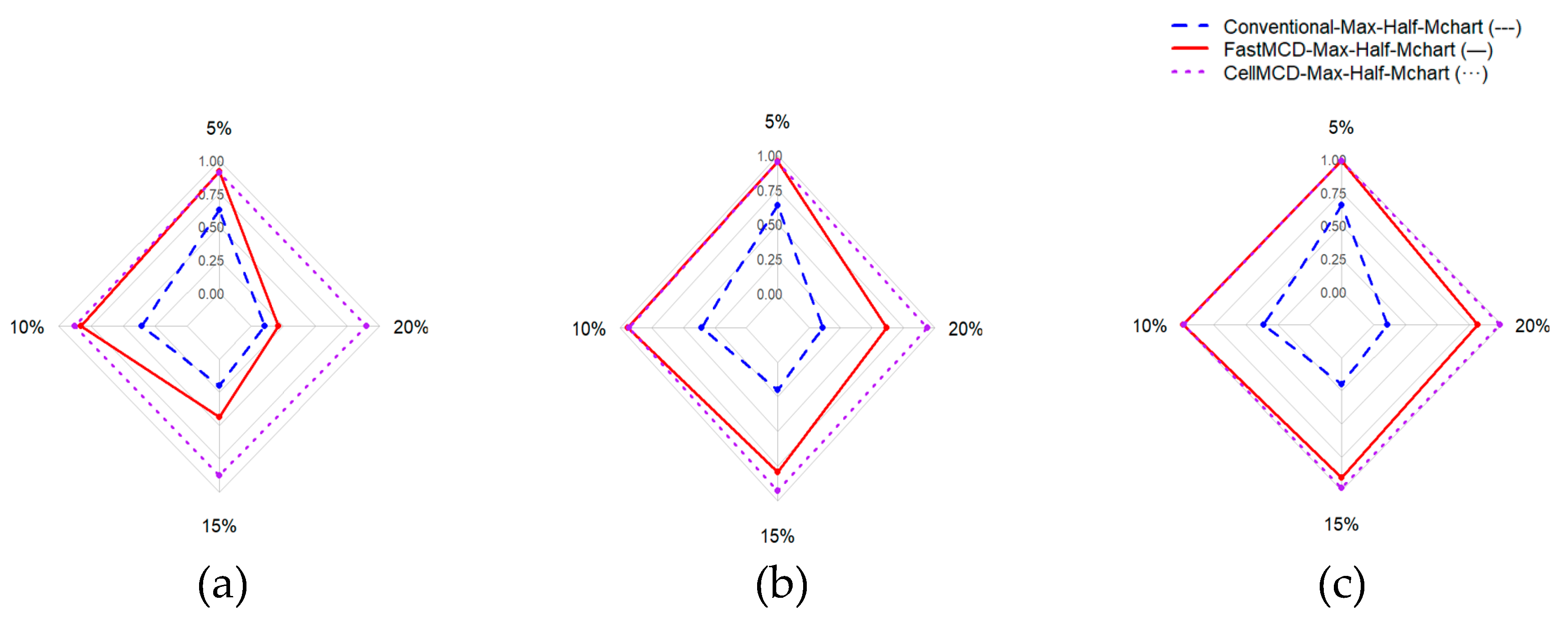
Figure 2.
FN Rate comparison for All Charts Based on Various Correlation (a) = 0.3, (b) = 0.5, and (c) = 0.7.
Figure 2.
FN Rate comparison for All Charts Based on Various Correlation (a) = 0.3, (b) = 0.5, and (c) = 0.7.
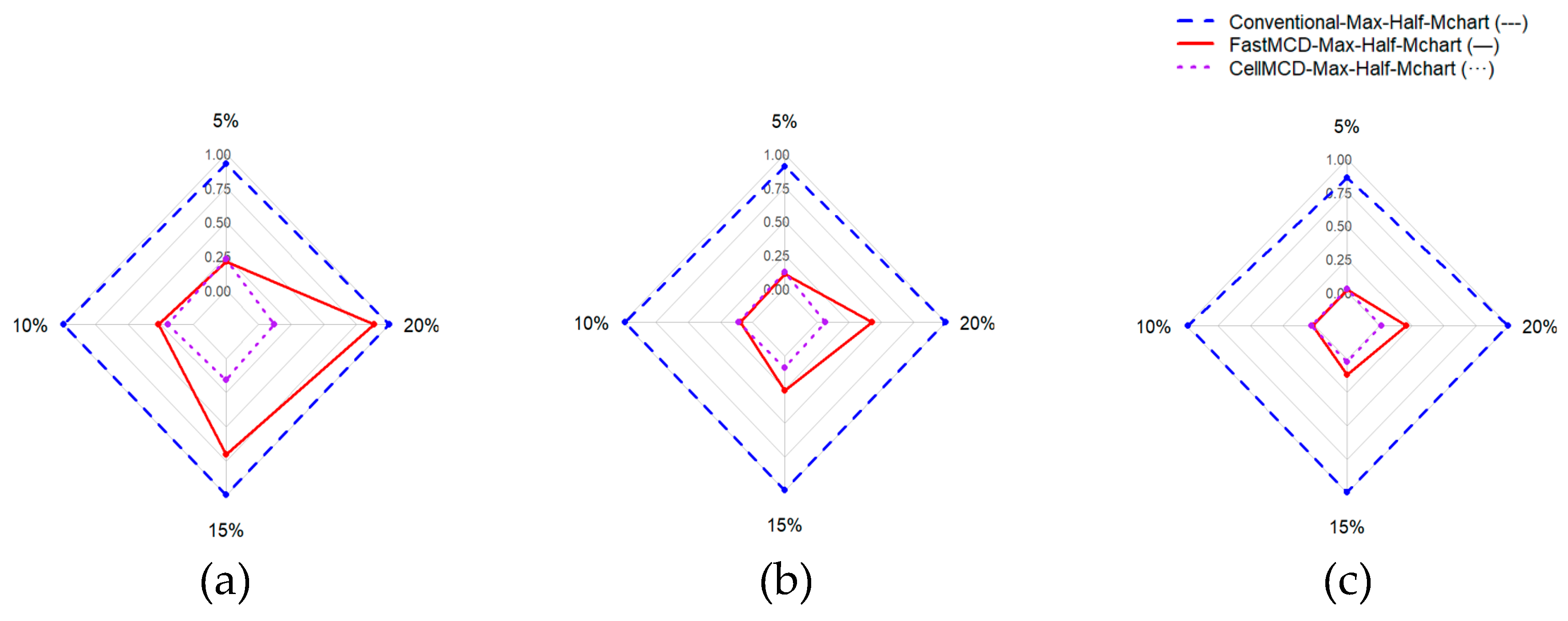
Figure 3.
AUC performance for All Charts Based on Various Correlation (a) = 0.3, (b) = 0.5, and (c) = 0.7.
Figure 3.
AUC performance for All Charts Based on Various Correlation (a) = 0.3, (b) = 0.5, and (c) = 0.7.
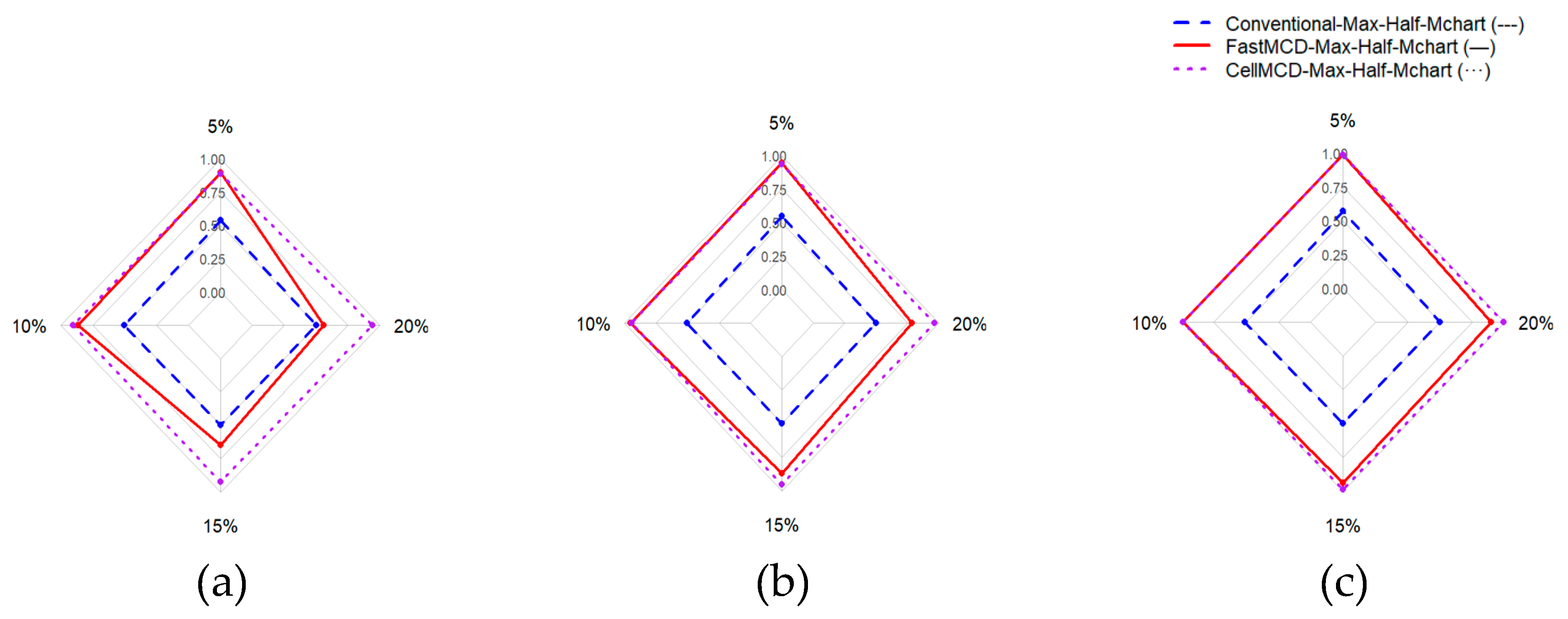
Figure 4.
Statistics Plot of Simulation on 5% outliers using (a) Max-Half-Mchart, (b) Max-Half-Mchart-FMCD, and (c) Max-Half-Mchart-cellMCD.
Figure 4.
Statistics Plot of Simulation on 5% outliers using (a) Max-Half-Mchart, (b) Max-Half-Mchart-FMCD, and (c) Max-Half-Mchart-cellMCD.

Figure 5.
Statistics Plot of Simulation on 15% outliers using (a) Max-Half-Mchart, (b) Max-Half-Mchart-FMCD, and (c) Max-Half-Mchart-cellMCD.
Figure 5.
Statistics Plot of Simulation on 15% outliers using (a) Max-Half-Mchart, (b) Max-Half-Mchart-FMCD, and (c) Max-Half-Mchart-cellMCD.
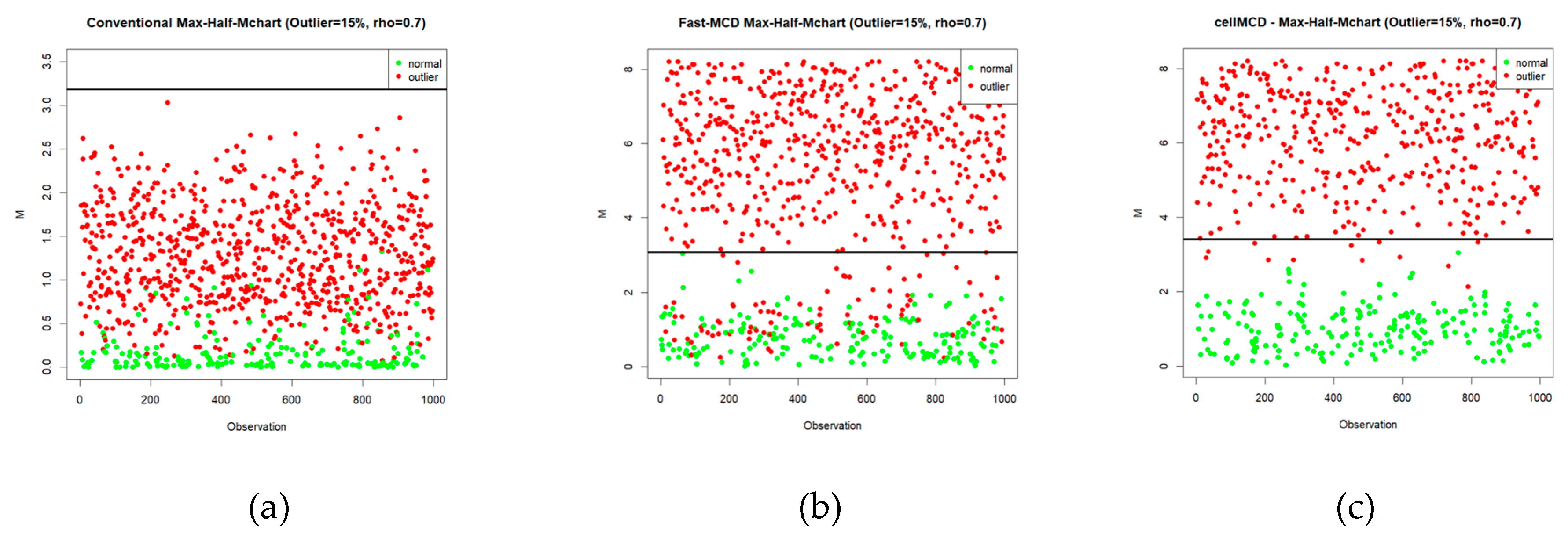
Figure 6.
Statistics Plot of Simulation on 20% outliers using (a) Max-Half-Mchart, (b) Max-Half-Mchart-FMCD, and (c) Max-Half-Mchart-cellMCD.
Figure 6.
Statistics Plot of Simulation on 20% outliers using (a) Max-Half-Mchart, (b) Max-Half-Mchart-FMCD, and (c) Max-Half-Mchart-cellMCD.
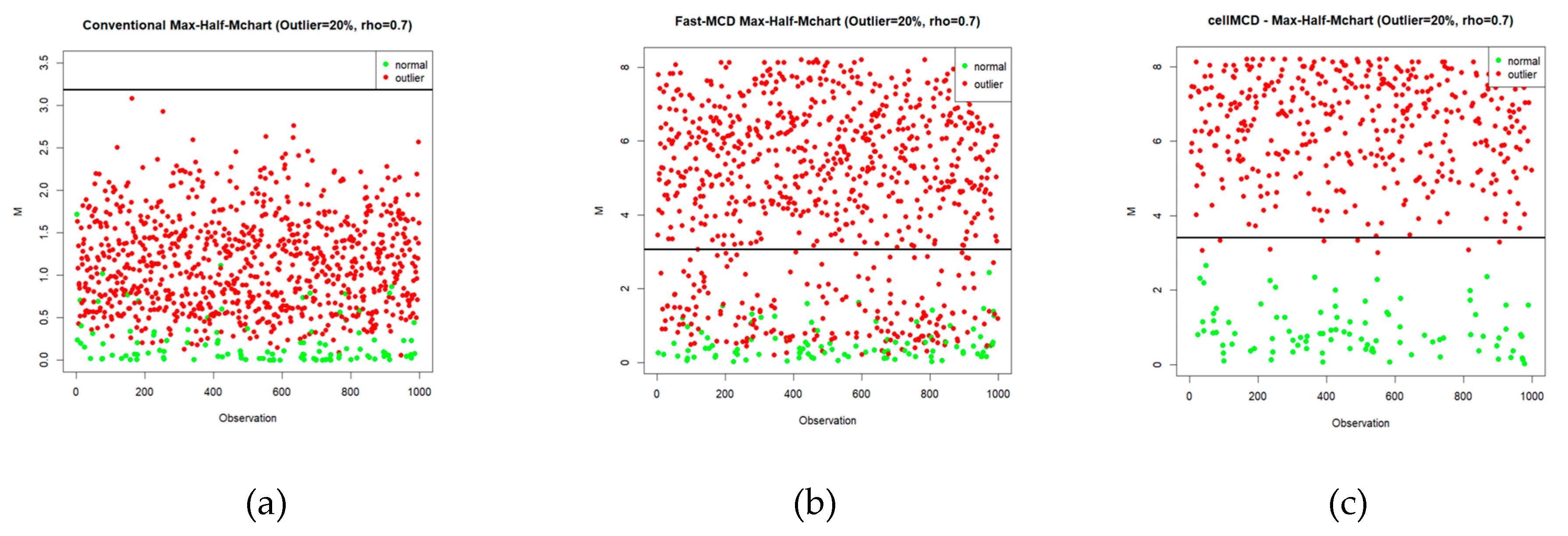
Figure 7.
Comparison ARL values of all charts: a) Mean shift, (b) Covariance matrix shift, and (c) both.
Figure 7.
Comparison ARL values of all charts: a) Mean shift, (b) Covariance matrix shift, and (c) both.
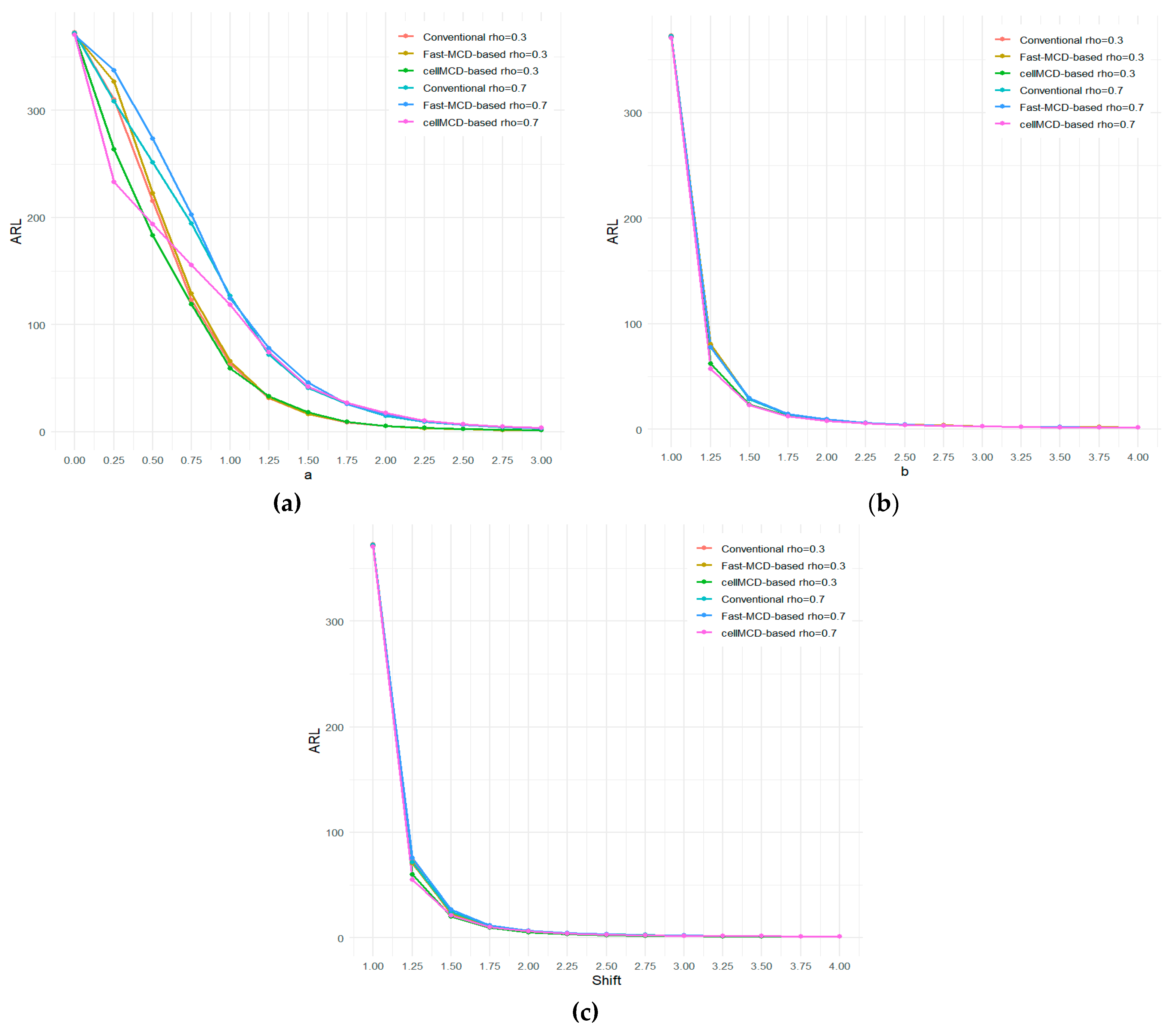
Figure 8.
Statistics plots of all charts under Scenario 1: a) Max-Half-Mchart, (b) Max-Half-Mchart-FMCD, and (c) Max-Half-Mchart-cellMCD.
Figure 8.
Statistics plots of all charts under Scenario 1: a) Max-Half-Mchart, (b) Max-Half-Mchart-FMCD, and (c) Max-Half-Mchart-cellMCD.
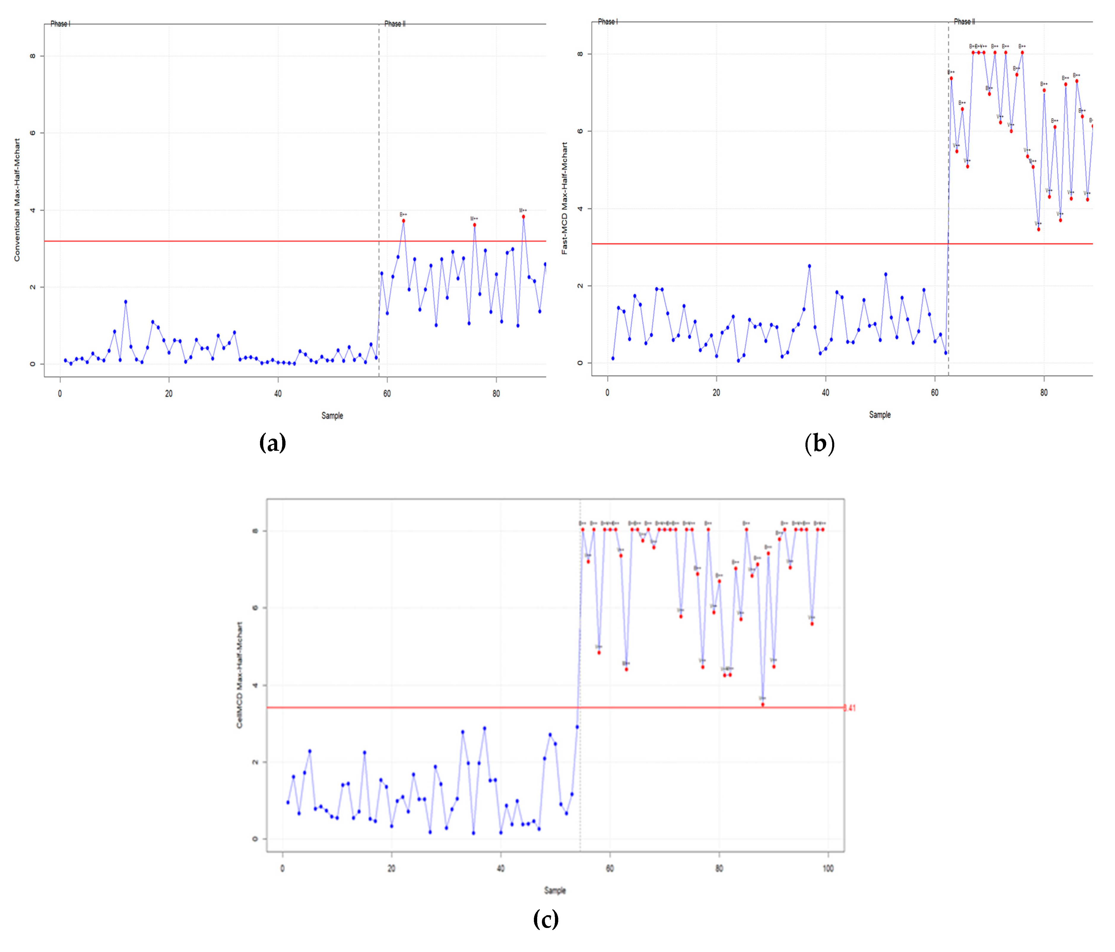
Figure 9.
Statistics plots of all charts under Scenario 2: a) Max-Half-Mchart, (b) Max-Half-Mchart-FMCD, and (c) Max-Half-Mchart-cellMCD.
Figure 9.
Statistics plots of all charts under Scenario 2: a) Max-Half-Mchart, (b) Max-Half-Mchart-FMCD, and (c) Max-Half-Mchart-cellMCD.
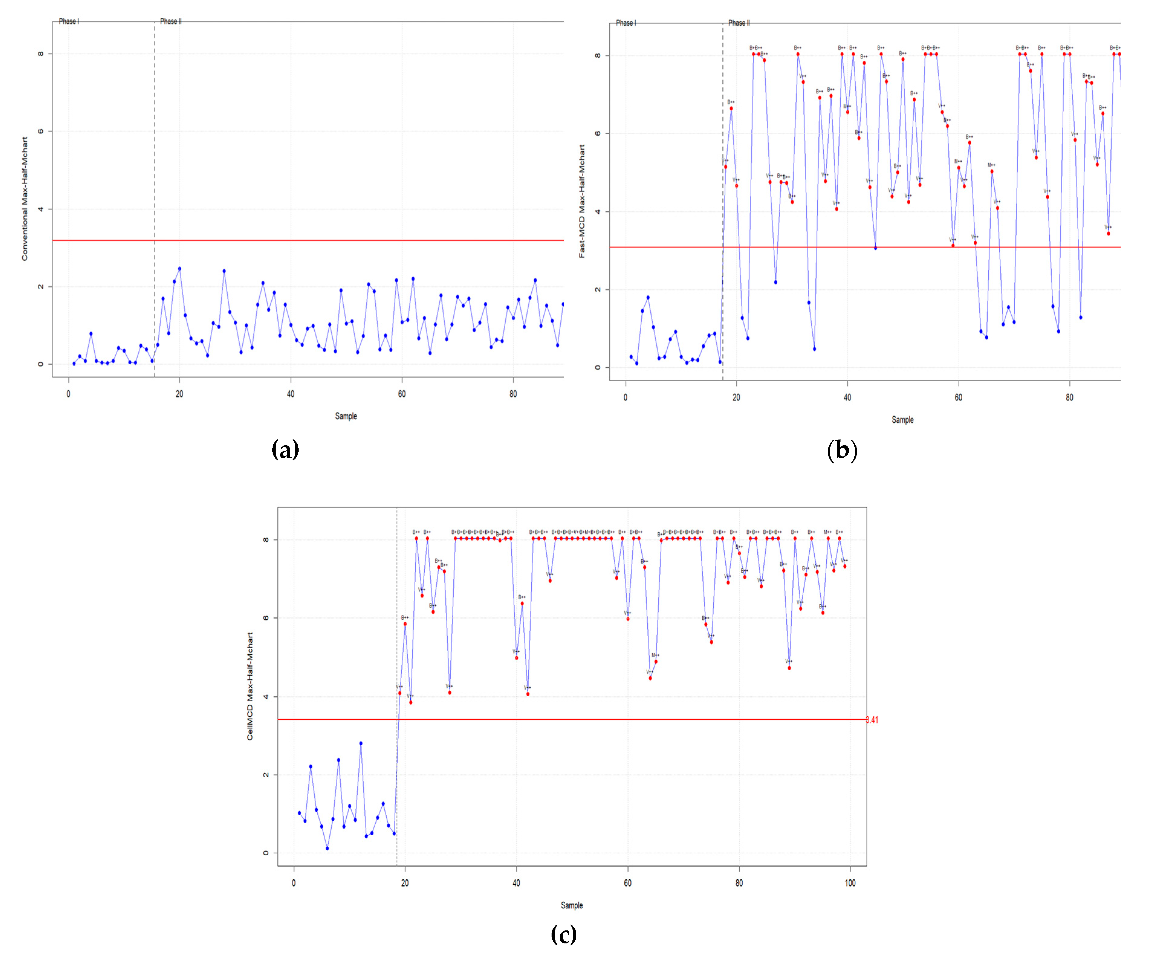
Figure 10.
Monitoring result of all charts under real datasets: (a) Conventional Max-Half-Mchart, (b) Fast-MCD-based Max-Half-Mchart, (c) cellMCD-based Max-Half-Mchart.
Figure 10.
Monitoring result of all charts under real datasets: (a) Conventional Max-Half-Mchart, (b) Fast-MCD-based Max-Half-Mchart, (c) cellMCD-based Max-Half-Mchart.
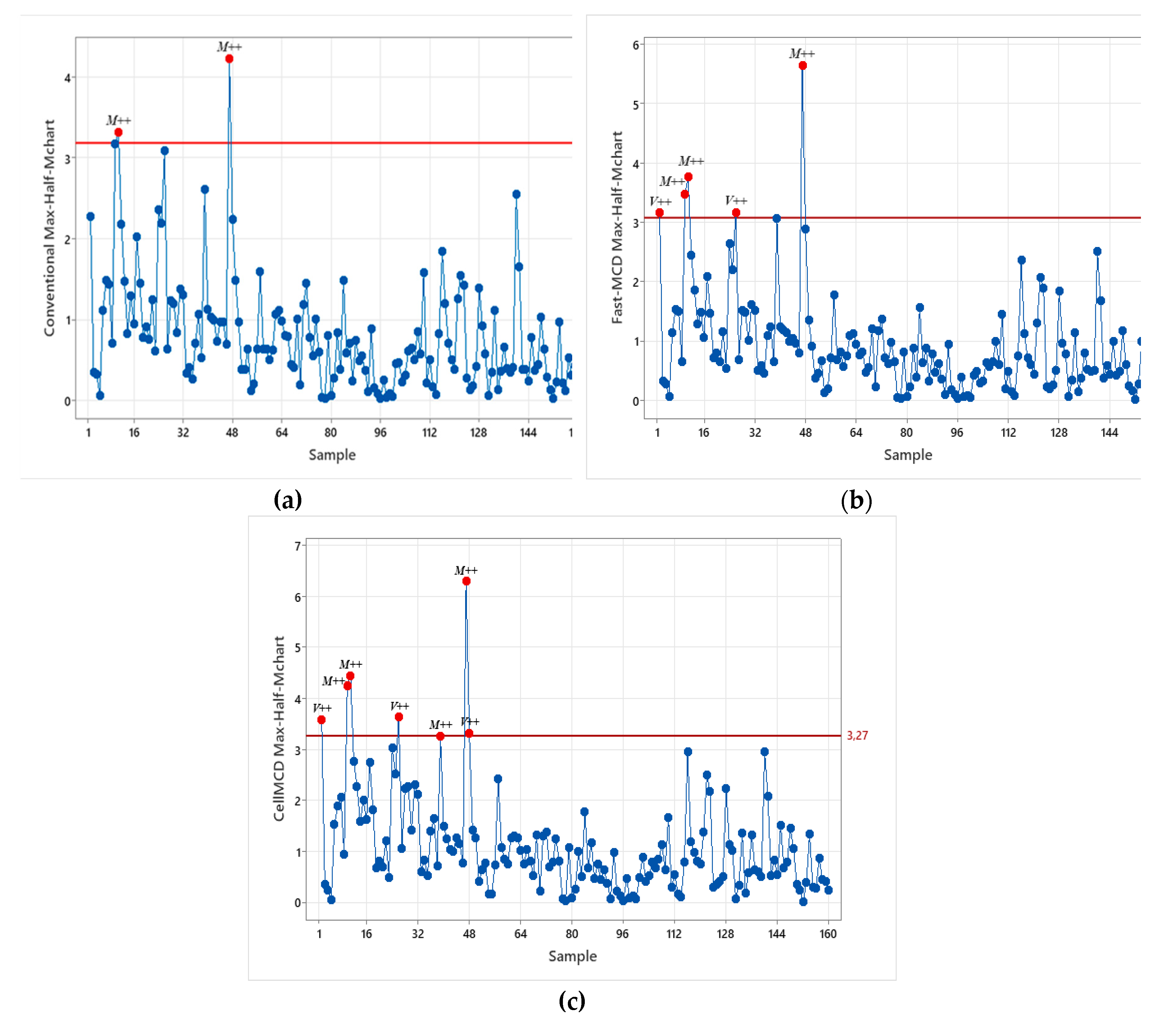
Table 2.
Simulation result for Conventional Max-Half-Mchart.
| ρ | %Out | Conventional Max-Half-Mchart | |||
|---|---|---|---|---|---|
| Accuracy | FP Rate | FN Rate | AUC | ||
| 0.3 | 5 | 0.6278 | 0.0000 | 0.9273 | 0.5363 |
| 10 | 0.3532 | 0.0000 | 0.9926 | 0.5037 | |
| 15 | 0.1977 | 0.0000 | 0.9992 | 0.5004 | |
| 20 | 0.1069 | 0.0000 | 0.9999 | 0.5001 | |
| 0.5 | 5 | 0.6366 | 0.0000 | 0.9044 | 0.5478 |
| 10 | 0.3559 | 0.0000 | 0.9892 | 0.5054 | |
| 15 | 0.1975 | 0.0000 | 0.9985 | 0.5007 | |
| 20 | 0.1076 | 0.0000 | 0.9997 | 0.5002 | |
| 0.7 | 5 | 0.6557 | 0.0000 | 0.8579 | 0.5710 |
| 10 | 0.3602 | 0.0000 | 0.9823 | 0.5089 | |
| 15 | 0.1984 | 0.0000 | 0.9975 | 0.5013 | |
| 20 | 0.1081 | 0.0000 | 0.9994 | 0.5003 | |
Table 3.
Simulation result for Max-Half-Mchart based on Fast-MCD.
| ρ | %Out | Fast-MCD–based Max-Half-Mchart | |||
|---|---|---|---|---|---|
| Accuracy | FP Rate | FN Rate | AUC | ||
| 0.3 | 5 | 0.9150 | 0.0025 | 0.2080 | 0.8948 |
| 10 | 0.8262 | 0.0008 | 0.2660 | 0.8666 | |
| 15 | 0.4353 | 0.0000 | 0.7018 | 0.6491 | |
| 20 | 0.2131 | 0.0000 | 0.8816 | 0.5592 | |
| 0.5 | 5 | 0.9559 | 0.0025 | 0.1059 | 0.9458 |
| 10 | 0.9390 | 0.0019 | 0.0925 | 0.9528 | |
| 15 | 0.7933 | 0.0001 | 0.2571 | 0.8714 | |
| 20 | 0.6166 | 0.0000 | 0.4293 | 0.7853 | |
| 0.7 | 5 | 0.9896 | 0.0025 | 0.0222 | 0.9877 |
| 10 | 0.9882 | 0.0023 | 0.0169 | 0.9904 | |
| 15 | 0.9067 | 0.0009 | 0.1160 | 0.9416 | |
| 20 | 0.8119 | 0.0002 | 0.2107 | 0.8945 | |
Table 4.
Simulation result for Max-Half-Mchart based on cellMCD.
| ρ | %Out | cellMCD–based Max-Half-Mchart | |||
|---|---|---|---|---|---|
| Accuracy | FP Rate | FN Rate | AUC | ||
| 0.3 | 5 | 0.9073 | 0.0019 | 0.2279 | 0.8851 |
| 10 | 0.8741 | 0.0015 | 0.1924 | 0.9031 | |
| 15 | 0.8764 | 0.0010 | 0.1535 | 0.9227 | |
| 20 | 0.8956 | 0.0008 | 0.1167 | 0.9413 | |
| 0.5 | 5 | 0.9495 | 0.0018 | 0.1231 | 0.9375 |
| 10 | 0.9301 | 0.0014 | 0.1064 | 0.9461 | |
| 15 | 0.9297 | 0.0011 | 0.0872 | 0.9558 | |
| 20 | 0.9400 | 0.0009 | 0.0671 | 0.9660 | |
| 0.7 | 5 | 0.9885 | 0.0020 | 0.0258 | 0.9861 |
| 10 | 0.9838 | 0.0015 | 0.0241 | 0.9872 | |
| 15 | 0.9836 | 0.0011 | 0.0202 | 0.9894 | |
| 20 | 0.9862 | 0.0011 | 0.0153 | 0.9918 | |
Table 7.
ARL of the cellMCD-Based Max-Half-MChart for and .
| a | b | ||||||||||||
|---|---|---|---|---|---|---|---|---|---|---|---|---|---|
| 1 | 1.25 | 1.5 | 1.75 | 2 | 2.25 | 2.5 | 2.75 | 3 | 3.25 | 3.5 | 3.75 | 4 | |
| 0 | 371.18 | 62.39 | 23.23 | 12.83 | 7.76 | 5.59 | 4.28 | 3.40 | 2.85 | 2.44 | 2.07 | 2.01 | 1.82 |
| 0.25 | 263.72 | 59.82 | 23.67 | 12.23 | 7.66 | 5.40 | 4.14 | 3.20 | 2.72 | 2.45 | 2.11 | 1.94 | 1.69 |
| 0.5 | 183.27 | 49.78 | 19.93 | 10.88 | 6.99 | 5.14 | 3.86 | 3.05 | 2.71 | 2.26 | 2.08 | 1.86 | 1.75 |
| 0.75 | 118.93 | 35.40 | 16.55 | 9.75 | 6.47 | 4.51 | 3.53 | 2.91 | 2.71 | 2.35 | 2.01 | 1.81 | 1.74 |
| 1 | 59.12 | 23.33 | 11.85 | 7.44 | 5.13 | 4.04 | 3.25 | 2.74 | 2.39 | 2.02 | 1.90 | 1.74 | 1.61 |
| 1.25 | 32.83 | 14.73 | 8.24 | 5.73 | 4.33 | 3.46 | 2.89 | 2.50 | 2.27 | 1.96 | 1.78 | 1.69 | 1.54 |
| 1.5 | 18.20 | 9.49 | 5.98 | 4.63 | 3.41 | 2.86 | 2.45 | 2.20 | 1.91 | 1.76 | 1.73 | 1.57 | 1.47 |
| 1.75 | 9.47 | 6.08 | 4.09 | 3.47 | 2.75 | 2.42 | 2.11 | 1.94 | 1.76 | 1.61 | 1.55 | 1.45 | 1.41 |
| 2 | 5.47 | 3.99 | 3.19 | 2.83 | 2.36 | 2.14 | 1.89 | 1.71 | 1.66 | 1.56 | 1.47 | 1.41 | 1.35 |
| 2.25 | 3.45 | 2.85 | 2.51 | 2.16 | 1.83 | 1.83 | 1.68 | 1.55 | 1.50 | 1.43 | 1.35 | 1.30 | 1.25 |
| 2.5 | 2.53 | 2.03 | 1.90 | 1.74 | 1.66 | 1.61 | 1.45 | 1.42 | 1.38 | 1.32 | 1.33 | 1.26 | 1.20 |
| 2.75 | 1.80 | 1.68 | 1.58 | 1.53 | 1.43 | 1.40 | 1.34 | 1.29 | 1.26 | 1.24 | 1.21 | 1.21 | 1.16 |
| 3 | 1.46 | 1.40 | 1.40 | 1.38 | 1.30 | 1.28 | 1.22 | 1.22 | 1.19 | 1.17 | 1.14 | 1.15 | 1.13 |
Table 11.
Performance Comparison of All Charts on Synthetic Data.
| Max-Half-Mchart | Scenario | Evaluation Metrics | |||
|---|---|---|---|---|---|
| Accuracy | FP Rate | FN Rate | AUC | ||
| Conventional | 1 | 0.6263 | 0.0000 | 0.9024 | 0.5488 |
| 2 | 0.1515 | 0.0000 | 1.0000 | 0.5000 | |
| Fast-MCD | 1 | 0.9798 | 0.0000 | 0.0541 | 0.9730 |
| 2 | 0.8182 | 0.0000 | 0.2195 | 0.8902 | |
| cellMCD | 1 | 0.9899 | 0.0182 | 0.0000 | 0.9909 |
| 2 | 0.9899 | 0.0000 | 0.0122 | 0.9939 | |
Disclaimer/Publisher’s Note: The statements, opinions and data contained in all publications are solely those of the individual author(s) and contributor(s) and not of MDPI and/or the editor(s). MDPI and/or the editor(s) disclaim responsibility for any injury to people or property resulting from any ideas, methods, instructions or products referred to in the content. |
© 2026 by the authors. Licensee MDPI, Basel, Switzerland. This article is an open access article distributed under the terms and conditions of the Creative Commons Attribution (CC BY) license.
Copyright: This open access article is published under a Creative Commons CC BY 4.0 license, which permit the free download, distribution, and reuse, provided that the author and preprint are cited in any reuse.


