Submitted:
23 February 2026
Posted:
26 February 2026
Read the latest preprint version here
Abstract
Handball performance analysis is still often conducted through manual review of match videos, while automation on broadcast footage remains challenging due to camera motion, strong perspective effects, and frequent occlusions during dense interactions. This study presents a practical and reproducible monocular pipeline for extracting handball analytics from a single broadcast viewpoint. Players are detected per frame, tracked over time, and projected onto a standardized handball court via homography-based camera calibration. The resulting court-referenced trajectories in metric units enable motion indicators such as distance covered and speed, along with coaching-oriented visual summaries including trajectory overlays and heatmaps. In addition, clip-level action recognition is performed using interpretable kinematic and scene-derived features and lightweight classifiers, with a comparative evaluation across multiple classical models. The modular design keeps intermediate steps explicit, supports reproducibility, and facilitates interpretation of both intermediate outputs and final analytics. Experiments on the UNIRI handball dataset demonstrate that meaningful performance analytics and action understanding can be obtained from single-camera broadcast video using transparent intermediate representations. This work highlights the practical potential of interpretable trajectory-based modeling for under-instrumented sports and provides a reproducible baseline for future extensions incorporating richer contextual cues.
Keywords:
handball analytics
; sports video analysis
; computer vision
; object detection
; multi-object tracking
; homography
; trajectory features
; action recognition
; visual analytics
1. Introduction and Background Information
Video based performance analysis is widely used across sports, but it often still depends on manual review and subjective tagging, especially when dedicated multi camera systems are not available. In sports such as football, basketball, and tennis, vision-based solutions are already integrated into professional workflows. Indicative examples include optical tracking platforms such as TRACAB and Second Spectrum, which provide detailed spatiotemporal data for tactical analysis and broadcast augmentation, as well as systems such as Hawk-Eye that support officiating and performance evaluation. These developments have enabled the introduction of advanced metrics, such as expected goals in football or spatial shot quality models in basketball, fundamentally altering how teams evaluate performance and make strategic decisions even for amateur events [29].
In contrast, team handball remains relatively underexplored in automated video-based analytics. Although it is a fast paced and tactically rich sport, it lacks the widespread availability of tracking data that exists in other sports. This gap is mainly explained by practical constraints. Multi camera tracking systems are expensive and are rarely deployed outside elite competitions. In addition, handball is played indoors on a relatively small court of 40 × 20 m, which leads to high player density and frequent physical contact. As a result, detections are often ambiguous, and occlusions are common. Finally, broadcast footage typically includes camera panning and zooming, as well as strong perspective changes, which makes stable spatial analysis more difficult.
Due to these conditions, many handball teams still rely on manual video review and basic event statistics. This limits the analysis of spatial structure, player movement, and tactical organization. Modern computer vision methods could extract rich spatiotemporal information even from single camera broadcast video, provided that the pipeline is designed to handle camera motion, perspective effects, and frequent occlusions.
Recent progress in sports analytics has been enabled by object detection and multi object tracking. One stage detector, such as the YOLO family, are often selected because they offer a practical balance between accuracy and speed. Tracking by detection methods then associate detections across frames to build trajectories that support motion analysis. SORT introduced a lightweight baseline, while DeepSORT extended it with appearance-based association and improved identity stability in crowded scenes [1,2]. To move beyond pixel coordinates, a common step is to map image positions to standardized court coordinates. This allows physically meaningful measurements, such as distance in meters and speed in meters per second, using a planar homography under the assumption that the playing surface is approximately planar.
Action recognition in team sports has been studied with deep spatiotemporal networks and with hybrid pipelines that incorporate pose, ball information, or trajectory representations. However, for less studied sports and limited datasets, interpretable feature-based classifiers remain a strong and practical baseline. They require fewer training samples, support clearer error analysis, and keep intermediate representations transparent. In this work, action recognition is treated as a comparative learning task at clip level using engineered descriptors, to quantify tradeoffs between classical model families under identical inputs and a common evaluation protocol.
Handball specific studies highlight the difficulty of broadcast conditions and the importance of tailored components. Prior work examined active player detection using activity measures [7] and explored dataset construction and action recognition using automatic annotation and classical motion features [8]. Despite these efforts, handball is still underrepresented in end-to-end single camera pipelines that connect detection, tracking, court mapping, and coach-oriented outputs under realistic broadcast conditions. Results are reported under a single fixed protocol and are compared against standard tracking and classification baselines, while prior handball studies are used primarily as methodological reference points due to differences in data, labels, and evaluation settings [1,2,7,8,10,11].
The main contributions of this paper are as follows:
- ○
- End-to-end pipeline for monocular handball analytics. We present a complete workflow that processes raw broadcast video into court-referenced trajectories, kinematic metrics, and coaching-oriented visual summaries.
- ○
- Spatial calibration to real-world coordinates. Using homography-based mapping to a standardized handball court, player movements are expressed in meters rather than pixels, enabling physically meaningful measurements and comparisons across clips.
- ○
- Interpretable action recognition. Action classification is performed using trajectory-derived kinematic features and lightweight, tree-based classifiers, prioritizing interpretability and robustness under limited data.
- ○
- Evaluation under real broadcast conditions. The framework is evaluated on annotated handball broadcast clips, highlighting both its strengths and its current limitations.
The remainder of this paper is organized as follows: Section 2 describes the proposed methodology. Section 3 presents the experimental setup, including dataset characteristics and evaluation metrics, and reports quantitative and qualitative results. Section 4 discusses the implications, strengths, and limitations of the proposed approach. Section 5 concludes the paper.
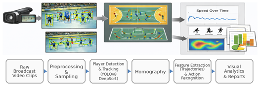
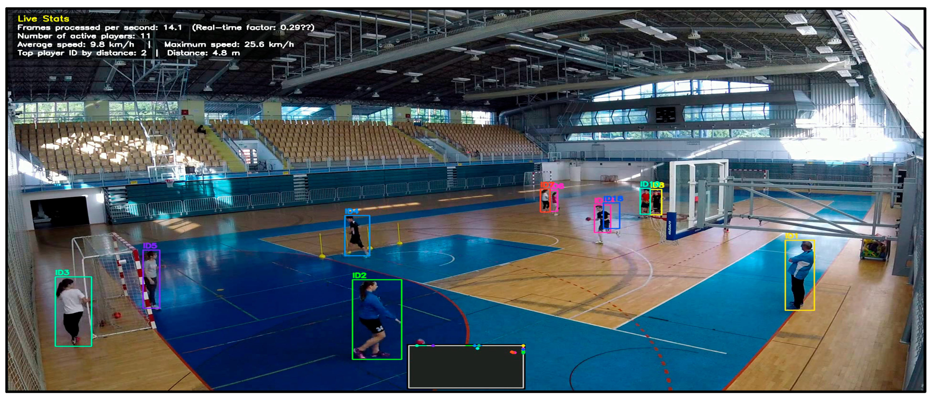
Figure 1.
Illustration of broadcast video analytics for performance assessment.
2. Materials and Methods
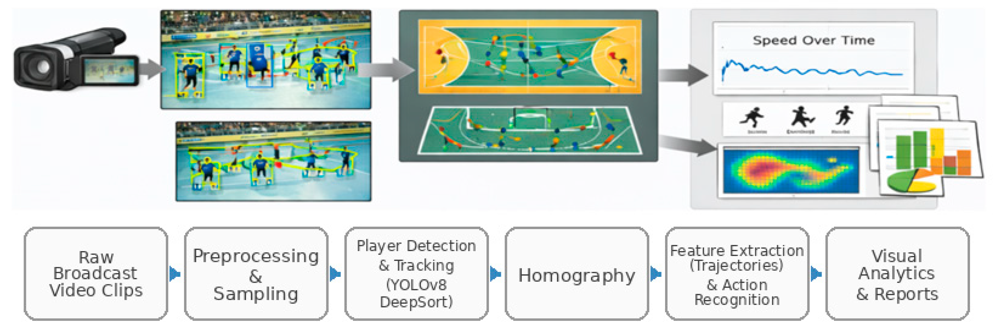
2.1. Overview of the Proposed Pipeline
The proposed workflow processes each video clip through a modular four-stage pipeline that produces explicit intermediate outputs at every step. Given a monocular broadcast clip , the goal is to transform pixel-level observations into court-referenced trajectories in metric units and to derive quantitative and visual analytics, along with clip-level action recognition.
In Stage 1, a deep detector is applied independently to each frame to localize players and output bounding boxes with confidence scores. In Stage 2, a tracking-by-detection method associates detections over time to form trajectories with persistent identities, enabling temporal continuity under short occlusions. In Stage 3, player image positions are mapped to a standardized court coordinate system using homography-based camera calibration under the planar court assumption, producing trajectories in meters.
In Stage 4, the court-referenced trajectories are used to compute motion indicators such as distance covered and speed, generate coaching-oriented visual summaries such as trajectory overlays and heatmaps, and extract interpretable clip-level features for action classification, which are evaluated with multiple lightweight classifiers under a common protocol.
A key design choice is modularity: each stage can be replaced independently while maintaining the same intermediate representations (detections, tracks, court-projected trajectories, and feature vectors). This structure supports reproducibility and systematic troubleshooting, since errors can be localized by inspecting the outputs of each stage before propagating to subsequent components.
Figure 2.
Overview of the proposed monocular handball analytics pipeline.
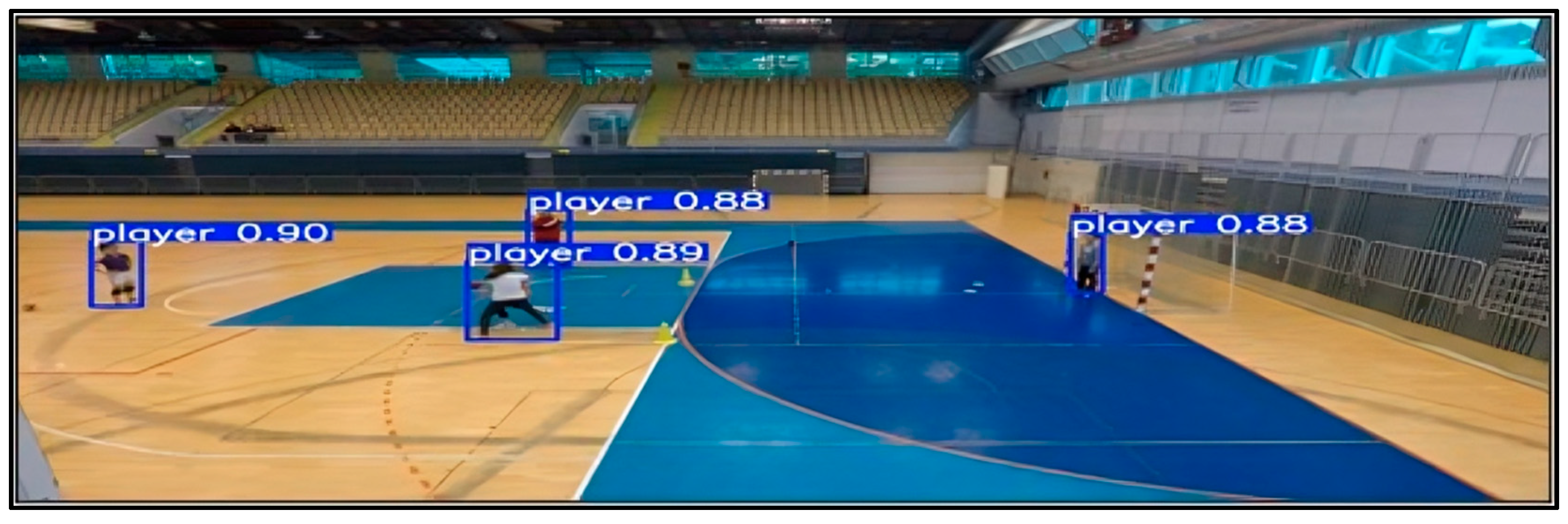
2.2. Player Detection and Tracking
Players are detected independently in each frame using a fine-tuned YOLOv8 model [3]. Given a frame , the detector returns a set of detections , where each detection includes a bounding box in pixel coordinates and a confidence score . The model is trained as a single-class detector (player) to maximize detection stability for subsequent tracking. At the level of internal feature extraction, the detector is treated as a black box, but its interface is explicit. For each frame it outputs a finite set of bounding boxes and confidence scores, which forms the observable input to the tracking stage.
To provide comparable inputs for the tracking stage, a fixed confidence threshold is selected on the validation set and then kept constant across all experiments. After thresholding, non-maximum suppression (NMS) is applied to remove duplicate detections. The overlap between two boxes A and B is quantified by the Intersection over Union . When exceeds a predefined NMS threshold, the lower-confidence detection is suppressed. Finally, detections are filtered with basic sanity checks to discard degenerate boxes, such as invalid dimensions or boxes outside image boundaries. The final output of Stage 1 is the per-frame detection set , which is passed unchanged to the tracker.
Figure 3.
Example of player detections in a broadcast frame (YOLOv8 outputs).
Frame-level detections are linked into trajectories using DeepSORT [2] under a tracking-by-detection paradigm. DeepSORT was selected because broadcast handball includes frequent short occlusions and close player interactions. In such conditions, appearance-based association reduces identity switches compared to purely motion-based trackers. This choice matters because identity instability and track fragmentation propagate to the downstream trajectory features and can degrade the reliability of clip-level action recognition.
The input to the tracker at time t is the per-frame detection set . The output is a set of tracks with persistent identities. For each track, the tracker provides a state estimate per frame, which includes the predicted location and bounding box in image coordinates. For each frame, the tracker maintains a set of active track identities . Each track state is propagated with a Kalman filter motion model, which predicts the next state and defines a motion-based gating region for plausible matches.
Data association combines spatial consistency with appearance similarity to reduce identity switches in crowded scenes and under short occlusions. Matching between predicted tracks and current detections is obtained by solving an assignment problem, typically with the Hungarian algorithm. This produces matched track–detection pairs, along with unmatched detections and unmatched tracks. Unmatched detections may initialize new tracks. Unmatched tracks may remain active for a limited number of frames, controlled by a maximum age parameter.
Tracking is performed independently for each clip because persistent identities across clips are not required for the downstream analytics. Conservative association settings are used to reduce false track initiations during dense interactions, prioritizing identity stability when players are in close proximity. The explicit track representation supports systematic troubleshooting because errors can be traced to missed detections, track fragmentation, or identity switches before court projection and motion analytics are applied.
2.3. Court Projection via Homography
To express movement in metric units, image coordinates are mapped onto a standardized 40×20 m handball court using a planar homography, under the assumption that the playing surface is approximately planar. A top-down court reference is used to reduce perspective effects and to make distances and speeds comparable across clips, regardless of camera zoom and viewpoint. This representation also supports coaching-oriented visualizations, such as trajectory overlays and heatmaps on the court template.
Let denote a point in image homogeneous coordinates (pixels) and let denote the corresponding point on the court template. The homography matrix satisfies the projective mapping where is a non-zero scale factor. The input to the homography estimation consists of image-to-court point correspondences derived from visible court landmarks, such as line intersections and characteristic marking points. The output is the 3×3 matrix H, which maps pixel coordinates to metric court coordinates and enables computation of kinematic quantities in meters and seconds.
For each tracked player, a single representative point is extracted from the bounding box and projected to the court plane. The bottom-center point is used as an approximation of the ground contact point. This choice reduces systematic perspective error compared to using the box center, which lies above the court plane. Court-referenced coordinates are obtained by applying the homography and converting from homogeneous to Euclidean coordinates, yielding positions in meters for each tracked identity and frame.
Calibration quality is verified through complementary checks. First, a visual overlay is performed by projecting the court template lines back onto the image and inspecting their alignment with visible markings. Second, plausibility checks are applied to the resulting trajectories and motion signals, including consistency with court bounds and speed values that remain within realistic ranges. When camera zoom or viewpoint changes significantly, a new homography must be estimated because a single planar homography cannot represent multiple camera geometries.
Figure 4.
Example of homography-based court projection to standardized coordinates.
2.4. Trajectory Processing and Motion Indicators
Court-referenced trajectories are post-processed to reduce high-frequency jitter introduced by detection and tracking noise, and to stabilize derivative quantities such as speed and acceleration. Let denote the projected court position in meters of track k at frame t. A short temporal smoothing filter is applied to the sequence } to suppress frame-to-frame fluctuations while preserving the overall motion pattern. This step is important because raw coordinate jitter can produce unrealistically large spikes in numerical derivatives. In practice, smoothing can be implemented using a short moving average or a low-pass filter applied independently to X and Y.
Motion indicators are then computed from the optionally smoothed trajectories. The distance covered by track k over the interval defined as the cumulative Euclidean displacement between consecutive points . Instantaneous speed is computed as displacement over time , where . Speed is expressed in meters per second. Clip-level speed statistics, such as mean, median, maximum, and percentiles, are computed per track and can also be aggregated across tracks to summarize the movement intensity within a clip.
To ensure physically plausible outputs, basic sanity checks are applied. Trajectory points are constrained to remain within court bounds, and unrealistic speed spikes are flagged as outliers and excluded from summary statistics when they exceed a plausible threshold. This filtering reduces the impact of occasional tracking fragmentation or identity switches on downstream motion analytics.
2.5. Visual Analytics Outputs
To support coaching-oriented interpretation, the pipeline produces court-referenced trajectory plots and heatmaps from projected trajectories in meters. Trajectory plots visualize the motion paths of tracked identities on a standardized 40×20 m court template. Each track is rendered as a polyline by connecting consecutive positions over time. When smoothing is enabled, the plotted paths reflect the stabilized trajectories and allow qualitative inspection of movement patterns such as runs, cuts, and positional changes.
Heatmaps provide a compact summary of spatial occupancy by aggregating projected positions over time and across tracked players. The court is discretized into a two-dimensional grid of cells, denoted as cell (m, n). For each cell, an unnormalized occupancy count is computed as in , where 1{⋅} is the indicator function. To reduce discretization artifacts and improve interpretability, H can be spatially smoothed and then normalized. A simple normalization divides by producing a relative occupancy distribution. The resulting heatmaps highlight frequently visited court regions and support qualitative comparisons between clips and action categories. Since heatmaps are derived from tracked and projected positions, their quality depends on tracking stability and calibration accuracy, especially under heavy occlusions and rapid camera motion.
2.6. Action Recognition Using Trajectory-Derived Features
Each clip is represented by a fixed-dimensional vector x that summarizes player motion on the court and the reliability of the underlying detections. The representation is computed from court-referenced trajectories and frame-level detection statistics. The resulting features remain physically interpretable and support diagnostic analysis when recognition errors occur. The feature set targets three aspects. Motion intensity and motion dynamics describe kinematics of play. Scene reliability describes how stable and consistent the detections are. This combination is useful in broadcast clips where viewpoint changes, occlusions, and variable scene density can mask action-specific motion patterns.
The projected court position of track k at frame t is denoted by in meters. The temporal sampling step is . For detections, denotes the number of detections in frame t, and the total number of detections across the clip is . Each bounding box provides width , height and confidence . From these, the box area and the aspect ratio are derived to capture apparent scale and shape consistency.
Trajectory-derived features are computed from consecutive projected positions and encode motion intensity and motion dynamics. The frame-to-frame displacement vector is , which describes how the player position changes between adjacent frames in the court plane. The displacement magnitude is which gives traveled distance per frame in meters. Instantaneous speed is then , transforming a geometric displacement into a physically meaningful rate of motion (m/s). To characterize direction, the motion angle is computed as , which yields a stable representation of direction on the court. Turning behavior is captured by the direction change . Large absolute values of correspond to sharper turns, while values near zero indicate approximately straight movement.
Because action labels are clip-level, per-frame quantities are aggregated to obtain a fixed-dimensional descriptor. Aggregation is performed in two stages to handle variability in the number of visible players. First, track-level summaries are computed over the temporal extent of each track. The distance covered by track k is , which measures how much the tracked identity moved during its presence in the clip.
Speed behavior is summarized per track using statistics of including mean speed, speed variability, maximum speed, and a high percentile such as the 90th percentile. These descriptors emphasize high-activity segments while remaining robust to occasional spikes. Directional dynamics are summarized similarly by computing statistics of ,the mean turning intensity quantifies how frequently and strongly a player changes direction, while captures variability in turning patterns.
Second, track-level values are pooled across tracks to form clip-level features. The mean and maximum distance across tracks, and , summarize typical and extreme movement within the clip. In parallel, global kinematic statistics are computed directly over all valid (t, k) pairs to capture clip-wide activity independent of track segmentation. These include the global mean speed , global variability and the global maximum . High-intensity bursts are summarized by the global percentile . Turning behavior at clip level is characterized by and . This two-level aggregation strategy produces a consistent feature vector even when some players are missing, tracks are fragmented, or the number of visible identities differs across clips.
Detection-derived features complement the motion descriptors by quantifying scene conditions and detection stability. Detection density is captured by the mean number of detections per frame and by its variability , which often increase under occlusions and crowded scenes. Geometric statistics of bounding boxes serve as proxies for camera zoom and scale changes. Mean and variability of box height and width , describe how large players appear in the image. Mean and variability of area provide an additional scale descriptor that is sensitive to both width and height. Shape consistency is captured by aspect-ratio statistics , which can reflect pose changes and partial occlusions. Finally, detection reliability is summarized by robust confidence descriptors: the median confidence reflects typical detector certainty, captures the upper tail of confident detections. Together, these features help disentangle genuine motion patterns from errors caused by unstable detections and provide additional context for interpreting classifier behavior.
To facilitate reproducibility, Table 1 summarizes the detection-derived features used in our clip-level representation. The features quantify detection density, bounding-box geometry, and confidence statistics aggregated over time. Since they are computed independently of the classifier, the same feature set is used across all evaluated models. Feature-importance analysis is presented in the Results section for the model that achieves the best overall performance.
The final feature vector x is used for clip-level action classification. The input to every classifier is the clip representation x. The output is a predicted action label among the predefined classes. When available, models also output class scores or posterior probabilities p (y ∣ x). The evaluated classifiers include Random Forest, Extra Trees, Logistic Regression, XGBoost, Gradient Boosting, and Gaussian Naive Bayes. Each model is trained with hyperparameter tuning on the training data using cross-validation. Class imbalance is handled using class weighting or balanced sample weights where supported. This feature-based formulation maintains interpretability throughout the pipeline and supports traceable error analysis by linking misclassifications to measurable properties of trajectories and detections.
All classifiers are trained and tuned under a single shared protocol. The training split is used for model fitting and cross-validation based hyperparameter selection. The validation split is used only when an explicit validation-based selection step is required, such as selecting the number of boosting rounds for boosted trees. Reporting and comparison of model performance are presented in the Results section using accuracy and macro-averaged metrics to account for class imbalance.
Model evaluation uses accuracy and macro-averaged precision, recall, and F1 score to account for class imbalance. The chosen metrics are defined as follows. For each class c, precision is defined as , and recall is . The class-wise F1 score is , and macro-averaged F1 is computed as , ensuring equal weighting across action categories regardless of frequency.
2.7. Evaluation Metrics
Performance is evaluated at three levels: detection, tracking, and action recognition.
For detection, we report precision, recall, and mean Average Precision. Precision and recall are defined using true positives, false positives, and false negatives as and A predicted detection is considered correct if its Intersection over Union (IoU) with the corresponding ground-truth bounding box exceeds a predefined threshold. For a predicted box A and a ground-truth box B, IoU is defined . Average Precision is computed as the area under the precision–recall curve, and mean Average Precision is obtained by averaging AP across classes. These metrics capture detection accuracy and sensitivity to missed players, particularly under occlusions and motion blur.
Tracking performance is evaluated using CLEAR MOT metrics, with emphasis on MOTA and IDF1 to reflect overall tracking quality and identity stability. Multi-Object Tracking Accuracy is defined as , where , , and denote the numbers of false negatives, false positives, and identity switches at frame t, respectively, is the number of ground-truth objects at frame t. Identity F1 measures identity consistency and is defined as , where IDTP, IDFP, and IDFN denote identity-based true positives, false positives, and false negatives.
Action recognition is evaluated using accuracy and macro-averaged precision, recall, and F1 score to account for class imbalance. For each class c, class-wise precision and recall are defined as and. The class-wise F1 score is then computed as. Macro-averaged scores are obtained by averaging class-wise values over all C classes. For example, macro-averaged F1 is defined as . In addition, confusion matrices are reported to visualize error patterns and highlight which action classes are most frequently confused. This evaluation setup supports systematic error analysis and helps link downstream recognition failures to upstream issues such as detection reliability, tracking stability, and court projection accuracy.
2.8. Implementation Details and Reproducibility
All clips are processed at a fixed spatial and temporal resolution of 960×540 pixels and 25 fps. Interlaced footage is deinterlaced prior to analysis to reduce motion artifacts that may affect detection and tracking. Each clip is processed independently using the same pipeline stages, namely detection, multi object tracking, court plane projection via homography, and action recognition. The same data splits and evaluation protocol are used across all experiments to ensure direct comparability.
To ensure reproducibility, operating parameters are selected on the validation set and then kept constant during testing. This includes the detector confidence threshold used to filter detections before tracking, as well as tracking parameters that control track initiation and termination under occlusions. When frame sub sampling with step s is applied, tolerance parameters are adjusted consistently to preserve comparable temporal behavior. The implementation is modular and produces explicit intermediate outputs, including per frame detections, per clip trajectories with persistent identities, and court projected trajectories in metric units. Configuration files store the experimental settings and enable exact replication of results, as also described in the Data Availability Statement.
In terms of runtime, the dominant cost is the detector. Using YOLOv8n on CPU with inference input size 512, after resizing the 960×540 frames for model inference, the validation run reports average speeds of 0.4 ms for preprocessing, 19.7 ms for inference, and 0.5 ms for postprocessing per frame, which corresponds to approximately 20.6 ms per frame for detection. This establishes an upper bound on the achievable throughput of the full pipeline, since subsequent stages operate on detector outputs and are computationally lighter. Detection cost scales primarily with input resolution, while tracking by detection increases with the number of active tracks and detections due to the association step. Homography projection is linear in the number of transformed points and is typically negligible after calibration. Action recognition cost depends mainly on the temporal window length and the feature dimensionality, with classifier inference remaining comparatively lightweight for shallow models.
3. Results
Experiments were conducted on the UNIRI Handball Dataset [6], which consists of monocular broadcast handball clips annotated with action labels. In the version used in this study, the dataset contains 751 clips comprising 59,641 frames. Each clip is associated with a single dominant action label, following a clip-level annotation scheme. Although the clips are annotated with a single dominant action label, each clip typically contains multiple players and interactions. The provided label refers to the clip as a whole and not to a specific tracked identity. Therefore, the pipeline detects and tracks all visible players and aggregates motion information across tracks to build a single clip-level representation for action recognition. This formulation aligns the learning target with the available supervision and supports the use of lightweight, interpretable classifiers on engineered clip descriptors. The dataset covers seven action categories: crossing, defence, dribbling, jump-shot, passing, running, and shot.
To reduce contextual leakage between training and evaluation, we applied a match-wise split, ensuring that clips originating from the same match do not appear in multiple subsets. The resulting partition includes 525 clips for training, 113 clips for validation, and 113 clips for testing. Since the class distribution is strongly imbalanced, evaluation for action recognition is reported using macro-averaged metrics, which assign equal importance to each action category irrespective of its frequency. All compared classifiers are trained and evaluated under this same split and metric protocol to ensure a fair comparison.
3.1. Player Detection Performance
This subsection reports the performance of the player detector under broadcast conditions, where rapid camera motion, motion blur, scale variation, and frequent inter-player occlusions make consistent localization challenging. On the evaluation split, the detector achieves precision 0.896 and recall 0.768, as summarized in Table 1. The high precision indicates that most predicted bounding boxes correspond to true players. This is desirable for downstream tracking because false positives often generate short-lived tracks and increase the likelihood of identity switches. The lower recall suggests that a noticeable fraction of players is missed. Misses occur primarily in dense scenes and during heavy occlusions, where partial visibility reduces detector confidence and leads to missed detections across frames.
Mean Average Precision further characterizes detection quality across confidence thresholds. The detector reaches mAP@0.5 of 0.858, indicating strong detection and localization performance under a moderate IoU requirement that is commonly sufficient for reliable track association. Under the stricter COCO-style metric mAP@0.5:0.95, performance decreases to 0.562, as expected. Higher IoU thresholds penalize even small localization errors. The gap between mAP@0.5 and mAP@0.5:0.95 suggests that most detections overlap the ground truth adequately for tracking, while bounding-box tightness and precise alignment remain limiting factors in difficult frames such as fast motion, partial occlusions, and small-scale players.
From a pipeline perspective, these results define a practical operating point. Prioritizing precision over recall is appropriate because false positives tend to be more harmful to tracking stability than occasional missed detections. Nevertheless, missed detections can cause track fragmentation when players are absent for consecutive frames. This propagates to court-projected trajectories as discontinuities and can reduce the reliability of motion-derived features used for action recognition. For this reason, the subsequent tracking and trajectory-processing stages incorporate robustness mechanisms, including association over short gaps and feature aggregation based on robust statistics, to mitigate the impact of intermittent misses.
Overall, the detector provides a reliable input for tracking and downstream analytics, with remaining errors concentrated in predictable broadcast-specific failure cases. Detection results are summarized in Table 2.
3.2. Multi-Object Tracking Performance
Tracking performance is evaluated using CLEAR MOT metrics to quantify overall association quality and identity stability across time. On the evaluation split, the tracker achieves MOTA 0.71 and IDF1 0.74, as summarized in Table 3. These values indicate that the system maintains coherent trajectories for a substantial portion of each clip, while still being affected by typical broadcast challenges such as occlusions, rapid camera motion, and dense player interactions.
Tracking precision reaches 1.00, indicating that the produced track associations are highly reliable, and that false positive tracks or spurious associations are rare in this configuration. This behavior is consistent with a conservative tracking regime, where track initiation and association are accepted only when matching confidence is sufficiently high. In contrast, tracking recall is 0.72, suggesting that the dominant source of error is missed associations rather than false associations. In practice, recall degradation is primarily caused by prolonged occlusions and tightly clustered formations, where detections become intermittent or ambiguous. These conditions lead to fragmented track segments and reduced trajectory continuity, which can propagate to downstream court-projected motion analysis. From a pipeline perspective, this precision–recall profile is appropriate for trajectory-based analytics. False tracks and identity switches tend to contaminate motion-derived features more severely than short gaps, which can be partially mitigated through robust aggregation and temporal filtering.
Figure 5(a) provides a clip-wise breakdown of tracking performance. Precision remains consistently near-perfect across clips, whereas MOTA, IDF1, and recall vary across action scenarios. This variation is expected because clips with higher interaction density and frequent occlusions impose stricter requirements on data association and identity maintenance. Overall, the clip-level results confirm that identity stability is reasonably preserved, while residual errors concentrate in visually challenging situations rather than being uniformly distributed.
Figure 5(b) examines the sensitivity of derived motion indicators to temporal sampling. The plot reports the estimated mean speed as a function of the frame step, while scaling DeepSORT temporal parameters accordingly to maintain a comparable association horizon. Even under this scaling, mean speed decreases as the frame step increases. Coarser sampling reduces temporal resolution and tends to underestimate path length when motion includes curved trajectories, short accelerations, or frequent direction changes. This observation is important for reproducibility. Motion features such as speed and turning are not invariant to sampling, so the temporal sampling strategy must be kept consistent across experiments. For fair comparisons, the same frame step and feature computation protocol should be used for all reported results.
3.3. Court Projection and Visual Analytics Outputs
Court projection converts image-plane tracks into a common metric reference frame, enabling movement interpretation in meters and consistent comparison across clips and action categories. After homography-based calibration, projected trajectories are expressed on a standardized 40 × 20 m court template. Motion indicators such as distance covered, speed percentiles, and turning intensity then reflect physical quantities rather than camera-dependent pixel measurements. This step is critical in broadcast settings because zoom and viewpoint changes would otherwise make image-space motion statistics difficult to interpret and not comparable between clips.
Beyond quantitative features, court projection also enables visual analytics for qualitative validation and coaching oriented interpretation. Trajectory plots provide a direct view of the spatial paths followed by tracked identities. Occupancy heatmaps summarize spatial utilization by accumulating projected positions over time, followed by smoothing and normalization. These heatmaps highlight frequently visited regions, reveal coarse tactical structure such as preferred zones and transitions, and act as a diagnostic tool. Localized artifacts, discontinuities, or implausible concentrations can indicate tracking fragmentation, identity switches, or calibration drift. Since these outputs depend on both tracking and projection, their interpretability requires stable detections, reliable identity maintenance, and accurate homography estimation, especially under heavy occlusion and rapid camera motion.
A representative heatmap is shown in Figure 6. The visualization reports a normalized density over the court plane, where brighter regions correspond to higher accumulated occupancy. To ensure fair comparisons, the same court coordinate system and normalization procedure are used throughout. When clips include attacks in opposite directions, the court coordinates are flipped so that the attacking direction is fixed, ensuring that left right asymmetries reflect movement tendencies rather than camera orientation. Since heatmaps and trajectory-based indicators rely on the geometric projection, projection reliability is assessed using manually annotated court landmark correspondences on a subset of evaluation clips. For N equals 20 clips, visible court intersections are annotated and mapped to their known template coordinates. For each annotated landmark, the homography projection is applied and the reprojection error is computed as the Euclidean distance between the projected point and the corresponding ground truth template point, reported in pixels. The mean reprojection error and its standard deviation are then calculated across all annotated landmarks and clips. Using the adopted court template and resolution, pixel errors can be approximately interpreted in metric units by using a reference scale of about 0.04 m per pixel in court space, so that 5 pixels correspond to about 0.2 m and 10 pixels correspond to about 0.4 m.
This level of geometric error is acceptable for motion indicators such as distance covered and average speed, where accumulated displacements typically exceed several meters. Overall, these results support the use of homography based projection as a reliable step for obtaining stable metric coordinates under broadcast conditions.
3.4. Action Recognition Results
Table 4 summarizes clip-level action recognition performance using the proposed trajectory-derived representation described in Section 2.8. Among the evaluated classifiers, Random Forest and Gradient Boosting achieve the strongest overall performance, both reaching an accuracy of 0.805. Random Forest attains the highest macro-F1 of 0.745, while Gradient Boosting yields a very similar macro-F1 of 0.743, indicating comparable effectiveness under the same feature representation and protocol. Extra Trees follows closely with an accuracy of 0.791 and a macro-F1 of 0.719, suggesting that increased split randomization leads to a small reduction in macro-averaged performance in this setting.
Boosting with XGBoost achieves an accuracy of 0.761 and a macro-F1 of 0.693, providing competitive performance but remaining below the best-performing tree ensembles in macro-averaged scores. Logistic Regression reaches an accuracy of 0.619 and a macro-F1 of 0.540, reflecting the limitations of a linear decision boundary for the proposed descriptors. Gaussian Naive Bayes yields an accuracy of 0.451 and a macro-F1 of 0.431, serving as a low-complexity probabilistic baseline under strong independence assumptions.
Because the dataset is class-imbalanced, macro-averaged precision, recall, and F1 are emphasized. Unlike accuracy, macro-averaged metrics assign equal weight to each class and therefore better reflect performance on minority categories. In this setting, Random Forest reaches macro-precision 0.813, macro-recall 0.712, and macro-F1 0.745. This indicates that the model generalizes reasonably well across categories, while recall remains weaker for rare actions.
Figure 7 reports the confusion matrix of the best-performing Random Forest classifier on the held-out test set. The strong diagonal structure indicates robust recognition for the most frequent categories. Jump-shot is recognized reliably, with 48 correct predictions. Crossing and passing also show stable performance, with 18 and 13 correct predictions, respectively.
The most prominent confusions occur between shot and jump-shot. Several shot instances are predicted as jump-shot, and a smaller number of jump-shot instances are predicted as shot. This behavior is consistent with broadcast footage, where the two actions may share similar short-term kinematic signatures. Camera zoom and viewpoint changes can further reduce the discriminative power of trajectory-only cues. Additional errors include crossing predicted as jump-shot, which can arise in fast transitions that exhibit high-speed bursts and abrupt direction changes.
Minority classes remain the main challenge. Categories with very low support, such as defence and running, yield few correct predictions. This directly lowers macro-recall and helps explain why macro-F1 remains substantially below accuracy.
The confusion matrix shows that most errors occur between kinematically similar actions, such as shot and jump shot, where the underlying player motion differs subtly, and ball-related cues are not explicitly modeled. Misclassifications are also more frequent for low-support classes, which reduces macro-recall and macro-F1. This suggests that additional cues, such as explicit ball tracking or richer temporal descriptors, could improve separation between visually similar actions.
Feature importance for Random Forest is shown in Figure 8 and indicates that scene-density and detection-stability descriptors play a major role in the model decisions. The most influential feature is count_mean, the mean detections per frame, which acts as a proxy for scene density and often correlates with crowded phases of play. High importance is also assigned to confidence percentiles such as conf_p90 and conf_med, as well as scale and shape statistics such as bbox_h_mean and bbox_ar_std. These features capture camera zoom effects and detection consistency under motion blur and partial occlusion.
Importantly, these importance scores reflect how strongly a feature is used by the model in this dataset and configuration and should not be interpreted as causal evidence. The prominence of scene-density and detection-stability descriptors suggests that part of the classification signal is linked to upstream detection and tracking reliability under specific viewing conditions, including crowding, zoom, and occlusion, rather than purely action-specific motion patterns. This observation motivates future extensions that incorporate more action-specific cues, such as longer temporal context or ball-related information, to reduce ambiguity between kinematically similar classes.
Across the evaluated clips, the pipeline produces stable court-referenced trajectories that support quantitative motion indicators and coaching-oriented visualizations. Homography-based calibration maps image-plane detections to a standardized 40 × 20 m court, enabling metric interpretation of movement and consistent comparison across clips.
Detection and tracking performance remain the primary drivers of downstream reliability. The detector operates in a high-precision regime, while missed detections and prolonged occlusions are the main sources of trajectory fragmentation. Tracking results indicate generally stable identity maintenance, with errors concentrated in dense and visually challenging scenes. These limitations propagate to projected trajectories and can increase sensitivity to calibration noise when detections become unstable.
Action recognition results show that the interpretable trajectory-derived feature set provides a practical baseline under broadcast conditions and limited labeled data. Tree-based ensembles achieve the strongest macro-averaged performance, with Random Forest and Gradient Boosting performing best overall, followed by Extra Trees. XGBoost provides competitive results but remains below the best-performing ensembles, while Logistic Regression and Gaussian Naive Bayes serve as weaker baselines for the proposed descriptors. The main confusions occur between kinematically similar actions, especially shot versus jump-shot, and class imbalance further increases difficulty for rare categories. Overall, the most promising improvements are expected from more robust tracking under occlusions and more stable court calibration, together with richer action cues that reduce ambiguity between similar motions.
4. Discussion
4.1. Explanation of Results and Implications
The results demonstrate that a modular monocular broadcast pipeline can reliably extract metrically consistent handball analytics, if detection and tracking maintain sufficient temporal stability. Under broadcast conditions, detection performance achieves precision 0.896 and recall 0.768, which provides a reliable input to the tracking stage. This matters because detection errors propagate directly to tracking and trajectory quality. Missed detections tend to create gaps that fragment trajectories, while false positives can introduce spurious short tracks and increase the risk of identity instability.
Tracking performance, with MOTA 0.71 and IDF1 0.74, indicates that identity consistency is generally maintained across many clips, but performance degrades in the most difficult situations. In handball, dense interactions and prolonged occlusions are frequent and can interrupt association over multiple frames. This behavior is reflected in tracking recall of 0.72 and in occasional trajectory fragmentation. These discontinuities reduce the reliability of motion indicators that rely on temporal continuity and can also weaken the stability of aggregated trajectory-derived features used for recognition.
Court projection is critical for interpretability because it converts image-plane tracks into a common metric coordinate system. Homography-based calibration enables movement indicators in meters and supports coaching-oriented visual outputs such as court-referenced trajectories and heatmaps. This step also enables consistent comparison across clips, since motion descriptors become less sensitive to camera zoom and viewpoint changes. In practice, calibration quality depends on the visibility of court landmarks and the magnitude of camera motion. When calibration is accurate, the resulting analytics align with meaningful tactical regions of the court rather than pixel coordinates. When calibration is imperfect, projection noise can distort trajectory geometry and inflate derived quantities such as speed and turning, especially when combined with tracking gaps.
Action recognition results indicate that interpretable kinematic and detection-derived features provide a practical baseline for clip-level classification under limited and imbalanced data. Among the evaluated models, tree-based ensembles achieve the strongest macro-averaged performance. Random Forest reaches accuracy 0.805 and macro-F1 0.745, while Gradient Boosting performs comparably with accuracy 0.805 and macro-F1 0.743. Extra Trees follows with accuracy 0.791 and macro-F1 0.719. XGBoost achieves accuracy 0.761 and macro-F1 0.693, whereas Logistic Regression and Gaussian Naive Bayes provide weaker baselines for the proposed descriptors. Overall, these outcomes suggest that the feature set captures informative motion cues, but confusion between visually and kinematically similar actions remains, particularly under occlusion and viewpoint variation and for low-support classes. This limitation is expected in broadcast settings where ball cues are not explicitly modeled and where tracking fragmentation can obscure action-specific motion patterns.
Overall, the findings support the hypothesis that modular components with explicit intermediate representations can deliver useful coaching-oriented analytics from broadcast footage. At the same time, the results clarify the main bottlenecks for further improvement. The dominant limitations are robust tracking under prolonged occlusion and more stable court calibration under fast camera motion. Addressing these issues is likely to improve both the quality of motion analytics and the discriminative power of trajectory-derived action recognition features.
4.2. Comparison with Related Works
Direct comparison with prior handball studies should be interpreted with care because experimental conditions are not fully aligned across datasets and pipelines. Differences in frame rates, camera viewpoints, annotation policies, label definitions, and evaluation splits can change both the difficulty of the task and the meaning of the reported metrics. In practice, studies may use the same metric name while measuring a different operational problem, such as player detection in controlled capture versus identity stability during multi object tracking in broadcast footage.
A major source of mismatch is the data acquisition setting and the intended output of each work. The UNIRI HBD line of work by Maja Ivašić-Kos and Mirko Pobar focuses on handball specific data creation and player centric labeling, including active player identification and annotation strategies that often rely on capture conditions different from broadcast video, including fixed viewpoint recordings [6,7,8]. These contributions are highly relevant for defining labels and building handball datasets, and they support detection-oriented evaluation and player selection criteria, but they do not define a single end to end broadcast protocol that jointly evaluates tracking, court projection, and downstream analytics under camera motion, zoom changes, motion blur, and dense occlusions.
Within this family of work, active player detection is typically addressed using handball specific cues and activity measures that help identify the most relevant players in a scene [7]. Related dataset construction approaches combine detector outputs with additional spatiotemporal cues to accelerate labeling and improve dataset consistency [8]. These directions align well with the present study at the level of label definition and annotation logic, but they are only partially comparable to a broadcast pipeline where identity continuity and calibration robustness can dominate the quality of trajectories and any downstream interpretation.
Other handball papers broaden the scope to movement analysis and action recognition, yet comparability remains limited because the representation and evaluation target differ. Movement analysis studies often focus on describing activities and motion patterns using deep learning, with their own annotation handling and experimental setup [9]. Action recognition work in handball scenes also varies in action taxonomy, clip definition, and dataset split strategy, which affects class balance and difficulty and makes headline numbers sensitive to protocol choices [12]. As a result, similarities in task naming do not necessarily translate to comparable experimental evidence.
Among the cited handball works, PlayNet is one of the closest to an integrated, real-time workflow because it aims to map video to play level categories using tracking related modeling and learned embeddings under latency constraints [10]. This makes it conceptually close in terms of “video to semantics” ambition, but it is not equivalent to a modular broadcast pipeline that explicitly evaluates intermediate representations such as identity consistent trajectories in metric units. The difference matters, because a modular design can separate upstream failure modes from downstream modeling limits and can support coaching oriented interpretation and targeted debugging.
A second line that differs in core representation is pose based reasoning. Monocular 3D pose estimation and tracking in handball shifts the intermediate representation from court plane trajectories to articulated body configuration and its temporal dynamics [11]. This can be powerful for fine grained action cues, but it changes the error budget and the evaluation lens, since pose quality, visibility, and scale become primary factors, while court plane calibration and metric trajectories play a different role. Consequently, pose based results are best treated as complementary rather than directly comparable to trajectory derived feature pipelines.
At the tracking layer, many sports systems still rely on standard online baselines such as SORT and DeepSORT, which combine Kalman filtering with assignment, and optionally appearance embeddings for re identification across short occlusions [1,2]. Tracking performance is commonly reported with CLEAR MOT metrics, which explicitly quantify identity switches and fragmentation, two failure modes that are especially critical in multi-player scenes [4]. Recent tracking by detection advances aim to improve identity continuity under occlusions and variable detection confidence, which are typical in broadcast sports, and therefore represent plausible upgrade paths for the tracking stage even when they are not handball specific [18,19,20,35]. Sports oriented MOT datasets further highlight that results can shift substantially across domains and protocols, reinforcing the need for caution when interpreting cross paper comparisons [21,22].
Court projection is typically formulated as homography based registration that maps image coordinates to field or court coordinates, enabling metric trajectories when calibration is stable. Handball specific broadcast calibration is less represented in the cited set, but methodologically close work in soccer proposes robust strategies for moving cameras, partial field visibility, and broadcast artifacts, including calibration and sequential homography estimation approaches [24,25,26]. End to end soccer pipelines that reconstruct game state and produce a top view representation further demonstrate how calibration, localization, and identity tracking can be integrated, and they are useful methodological references even if they are not appropriate as direct handball benchmarks [23]. Homography estimation methods that improve robustness when classical feature matching is unreliable are also relevant in the same methodological sense [28].
In contrast, the present work evaluates a complete monocular pipeline on broadcast footage under a single fixed protocol across stages. The evaluation covers player detection, multi object tracking assessed with CLEAR MOT metrics [4], homography based court projection that yields trajectories in metric units, and clip level action recognition using interpretable trajectory derived features. The central contribution is the modular design with explicit intermediate representations, which supports coaching oriented interpretation and systematic error analysis by tracing downstream failures to concrete upstream causes, including missed detections, identity fragmentation typical of SORT and DeepSORT style tracking, and calibration noise from projection [1,2]. Therefore, the proposed evaluation is not positioned as a direct leaderboard comparison with prior handball studies, but as a controlled assessment of how errors propagate across detection, identity tracking, projection, and action recognition under broadcast constraints.
4.3. Limitations
This study is evaluated on broadcast handball footage, where performance can degrade under heavy player occlusions, rapid viewpoint changes, and zoom events that affect court calibration and tracking stability. Court projection relies on homography estimation, which becomes less reliable when court markings are only partially visible or when camera motion is abrupt. In such cases, projection noise can distort trajectories and influence derived motion indicators such as speed and turning.
Tracking quality also depends strongly on detector performance. Missed detections can interrupt associations, fragment trajectories, and reduce the continuity required for stable motion descriptors. Although high precision limits spurious tracks, reduced recall in dense scenes remains a practical source of downstream errors.
The action recognition component relies primarily on trajectory-derived motion features and is constrained by the available labeled data and class imbalance. As a result, rare action categories remain challenging, and generalization may be limited across competitions, camera setups, and filming conditions. In addition, the current representation does not explicitly model ball context or fine-grained pose cues, which can increase ambiguity between actions with similar movement patterns.
Finally, the reported results are tied to the adopted data split and evaluation protocol. While these are kept fixed for comparability across stages, alternative splits or more diverse datasets could lead to different performance profiles and may change which failure modes dominate.
4.4. Future Work
Future work can improve robustness and extend the analytics in several directions. Tracking can be strengthened under heavy occlusion by using improved re-identification, explicit occlusion handling, and camera motion compensation. These additions can reduce identity switches and trajectory fragmentation. Integrating appearance cues more effectively with motion-based association is also expected to increase tracking recall in dense interactions.
Court calibration can be made more scalable by reducing manual effort and improving stability under viewpoint changes. One direction is automatic or semi-automatic detection of court key points, followed by robust homography estimation that remains stable during zoom events and rapid camera motion. Temporal smoothing of calibration parameters across frames can further reduce projection jitter and improve the reliability of metric trajectories.
Action discrimination and event understanding can be enhanced by incorporating cues beyond player trajectories. Ball detection and ball–player interaction signals would help disambiguate actions with similar kinematic patterns. Broader context, such as team formation descriptors or phase-of-play indicators, could also improve recognition and support richer tactical analytics.
Finally, with larger labeled datasets, stronger temporal modeling can be explored for action recognition, including sequence-based classifiers that explicitly capture motion evolution over time. Such models should be introduced in a controlled way that preserves interpretability. This can be supported through feature attribution, systematic error analysis, and a fixed evaluation protocol to maintain reproducibility.
5. Conclusions
This study presented a practical and reproducible monocular pipeline for handball analytics from broadcast video. The workflow combines deep player detection, multi-object tracking, and homography-based court projection to obtain court-referenced trajectories in metric units. These trajectories support motion indicators and coaching-oriented visual summaries. They also enable clip-level action recognition using an interpretable set of trajectory-derived descriptors.
Experiments on the UNIRI handball dataset show that meaningful analytics can be extracted from broadcast footage using modular components and explicit intermediate representations. Beyond enabling systematic error analysis across stages, the approach is suitable for realistic settings where multi-camera systems and dense sensor setups are not available. Overall, the proposed pipeline provides a strong baseline for future handball-focused sports analytics and offers a clear foundation for extensions that improve robustness under occlusions, strengthen calibration stability, and enrich action understanding with additional cues. By keeping intermediate representations explicit and modular, the framework offers a transparent and extensible baseline for broadcast handball analytics that can be systematically improved as more robust components and richer cues become available.
Author Contributions
Kosmas Katsioulas and Ilias Maglogiannis contributed to the study’s conception, experimental design, data analysis, writing, and critical revisions, and approved the final manuscript. All authors have read and agreed to the published version of the manuscript.
Funding
This research received no external funding.
Institutional Review Board Statement
Not applicable.
Informed Consent Statement
Not applicable.
Data Availability Statement
The source code used in this study is available at: https://github.com/kkats96/Spatio-Temporal-Analysis-of-Handball-Players-using-Deep-Learning. The dataset used in this work is publicly available as UNIRI-HBD at IEEE DataPort: https://doi.org/10.21227/0g0a-fe06.
Acknowledgments
The authors acknowledge the support of the M.Sc. Program Information Systems and Services at the University of Piraeus, track Big Data and Analytics, for providing an inspiring academic environment and opportunities for collaboration. The authors also thank their families and close friends for their encouragement and support.
Conflicts of Interest
The authors declare no conflict of interest.
References
- Bewley, A.; Ge, Z.; Ott, L.; Ramos, F.; Upcroft, B. Simple online and realtime tracking. In Proceedings of the IEEE International Conference on Image Processing, ICIP, Phoenix, AZ, USA, 25–28 September 2016; pp. 3464–3468. [CrossRef]
- Wojke, N.; Bewley, A.; Paulus, D. Simple online and realtime tracking with a deep association metric. In Proceedings of the IEEE International Conference on Image Processing, ICIP, Beijing, China, 17–20 September 2017; pp. 3645–3649. [CrossRef]
- Ultralytics. Ultralytics YOLOv8. 2023. Available online: https://github.com/ultralytics/ultralytics.
- Bernardin, K.; Stiefelhagen, R. Evaluating multiple object tracking performance: The CLEAR MOT metrics. EURASIP Journal on Image and Video Processing 2008, 246309. [CrossRef]
- Breiman, L. Random forests. Machine Learning 2001, 45, 5–32. [CrossRef]
- Ivašić-Kos, M.; Pobar, M. Handball action dataset, UNIRI-HBD. IEEE DataPort 2021. [CrossRef]
- Pobar, M.; Ivašić-Kos, M. Active player detection in handball scenes based on activity measures. Sensors 2020, 20, 1475. [CrossRef]
- Ivašić-Kos, M.; Pobar, M. Building a labeled dataset for recognition of handball actions using Mask R-CNN and STIPS. In Proceedings of the 7th European Workshop on Visual Information Processing, EUVIP, Marrakesh, Morocco, 25–28 November 2018. [CrossRef]
- Host, K.; Pobar, M.; Ivašić-Kos, M. Analysis of movement and activities of handball players using deep neural networks. Journal of Imaging 2023, 9(3), 60. [CrossRef]
- Mures, O. A.; Taibo, J.; Padrón, E. J.; Iglesias-Guitian, J. A. PlayNet: real-time handball play classification with Kalman embeddings and neural networks. The Visual Computer 2024, 40(4), 2695–2711. [CrossRef]
- Sajina, R.; Ivašić-Kos, M. 3D pose estimation and tracking in handball actions using a monocular camera. Journal of Imaging 2022, 8(11), 308. [CrossRef]
- Host, K.; Ivašić-Kos, M.; Pobar, M. Action recognition in handball scenes. Lecture Notes in Networks and Systems 2022, 283, 645–656. [CrossRef]
- Kawamura, R.; Yamamoto, Y. Classification of handball shot through image analysis. In Proceedings of the International Conference on ICT and Knowledge Engineering, ICTKE, 2022. [CrossRef]
- Poovaraghan, R. J.; Prabhavathy, P. Advanced active player tracking system in handball videos using multi-deep sort algorithm with GAN approach. International Journal of Advanced Computer Science and Applications 2024, 15(7), 1191–1202. [CrossRef]
- Bassek, M.; Memmert, D.; Rein, R. Automatic formation recognition in handball using template matching. Lecture Notes on Data Engineering and Communications Technologies 2024, 209, 10–17. [CrossRef]
- Nicolosi, S.; Quinto, A. M. V.; Lipoma, M.; Sgrò, F. Situational analysis and tactical decision-making in elite handball players. Applied Sciences 2023, 13(15), 8920. [CrossRef]
- Lokas, I.; Vasilj, M.; Skender, S.; Vučetić, V.; Mihaldinec, H.; Džapo, H. Video-based jump height estimation in athletic performance testing. In Proceedings of the IEEE International Workshop on Sport, Technology and Research, STAR, 2023; pp. 39–44. [CrossRef]
- Zhang, Y.; Sun, P.; Jiang, Y.; Yu, D.; Weng, F.; Yuan, Z.; Luo, P.; Liu, W.; Wang, X. ByteTrack: multi-object tracking by associating every detection box. In Proceedings of the European Conference on Computer Vision, ECCV, 2022; pp. 1–21. [CrossRef]
- Du, Y.; Zhao, Z.; Song, Y.; Zhao, Y.; Su, F.; Gong, T.; Meng, H. StrongSORT: make DeepSORT great again. IEEE Transactions on Multimedia 2023, 25, 8725–8737. [CrossRef]
- Cao, J.; Pang, J.; Weng, X.; Khirodkar, R.; Kitani, K. Observation-centric SORT: rethinking SORT for robust multi-object tracking. In Proceedings of the IEEE CVF Conference on Computer Vision and Pattern Recognition, CVPR, 2023. [CrossRef]
- Cui, Y.; Zeng, C.; Zhao, X.; Yang, Y.; Wu, G.; Wang, L. SportsMOT: a large multi-object tracking dataset in multiple sports scenes. In Proceedings of the IEEE CVF International Conference on Computer Vision, ICCV, 2023; pp. 9887–9897. [CrossRef]
- Scott, A.; Uchida, I.; Ding, N.; et al. TeamTrack: a dataset for multi-sport multi-object tracking in full-pitch videos. In Proceedings of the IEEE CVF Conference on Computer Vision and Pattern Recognition Workshops, CVPRW, 2024; pp. 3357–3366. [CrossRef]
- Somers, V.; Joos, V.; Cioppa, A.; et al. SoccerNet game state reconstruction: end-to-end athlete tracking and identification on a minimap. In Proceedings of the IEEE CVF Conference on Computer Vision and Pattern Recognition Workshops, CVPRW, 2024. [CrossRef]
- Theiner, J.; Ewerth, R. TVCalib: camera calibration for sports field registration in soccer. In Proceedings of the IEEE CVF Winter Conference on Applications of Computer Vision, WACV, 2023; pp. 1166–1175. [CrossRef]
- Claasen, P. J.; de Villiers, J. P. Video-based sequential Bayesian homography estimation for soccer field registration. Expert Systems with Applications 2024, 252, 124156. [CrossRef]
- Shi, F.; Marchwica, P.; Gamboa Higuera, J. C.; Jamieson, M.; Javan, M.; Siva, P. Self-supervised shape alignment for sports field registration. In Proceedings of the IEEE CVF Winter Conference on Applications of Computer Vision, WACV, 2022; pp. 3768–3777. [CrossRef]
- Poovaraghan, R. J.; Prabhavathy, P. Deep YOLOv8-based handball detection system with transfer learning approach. Journal of Theoretical and Applied Information Technology 2023, 101(22), 7411–7424. DOI: not available.
- Nousias, G.; Delibasis, K. K.; Maglogiannis, I. G. Intelligent sampling consensus for homography estimation in football videos using featureless unpaired points. IEEE Access 2025, 13, 187843–187857. [CrossRef]
- Mavrogiannis, P.; Maglogiannis, I. Amateur football analytics using computer vision. Neural Computing and Applications 2022, 34, 19639–19654. [CrossRef]
- Zhao, Y.; Lv, W.; Xu, S.; Wei, J.; Wang, G.; Dang, Q.; Liu, Y.; Chen, J. DETRs beat YOLOs on real-time object detection. In Proceedings of the IEEE CVF Conference on Computer Vision and Pattern Recognition, CVPR, 2024. [CrossRef]
- Wang, A.; Chen, H.; Liu, L.; Chen, K.; Lin, Z.; Han, J.; Ding, G. YOLOv10: real-time end-to-end object detection. arXiv 2024. [CrossRef]
- Wang, C.-Y.; Yeh, I.-H.; Liao, H.-Y. M. YOLOv9: learning what you want to learn using programmable gradient information. arXiv 2024. [CrossRef]
- Wang, L.; Huang, B.; Zhao, Z.; et al. VideoMAE V2: scaling video masked autoencoders with dual masking. In Proceedings of the IEEE CVF Conference on Computer Vision and Pattern Recognition, CVPR, 2023. [CrossRef]
- Wang, Y.; Li, K.; Li, X.; et al. InternVideo2: scaling foundation models for multimodal video understanding. In Computer Vision, ECCV 2024, Lecture Notes in Computer Science, 2024. [CrossRef]
- Aharon, N.; Orfaig, R.; Bobrovsky, B.-Z. BoT-SORT: robust associations multi-pedestrian tracking. arXiv 2022. [CrossRef]
- Bochkovskiy, A.; Wang, C.-Y.; Liao, H.-Y. M. YOLOv4: optimal speed and accuracy of object detection. arXiv 2020. [CrossRef]
- Carreira, J.; Zisserman, A. Quo vadis, action recognition? a new model and the Kinetics dataset. In Proceedings of the IEEE Conference on Computer Vision and Pattern Recognition, CVPR, 2017; pp. 6299–6308. [CrossRef]
- Girdhar, R.; Carreira, J.; Doersch, C.; Zisserman, A. Video action transformer network. In Proceedings of the IEEE Conference on Computer Vision and Pattern Recognition, CVPR, 2019; pp. 244–253. [CrossRef]
- Xarles, A.; Escalera, S.; Moeslund, T. B.; Clapés, A. ASTRA: an action spotting TRAnsformer for soccer videos. In Proceedings of the ACM International Conference on Multimedia Workshops, 2023. [CrossRef]
- Shorten, C.; Khoshgoftaar, T. M. A survey on image data augmentation for deep learning. Journal of Big Data 2019, 6(1), 60. [CrossRef]
Figure 5.
Tracking evaluation: (a) per-clip MOT metrics; (b) sensitivity of estimated mean speed to frame sampling (frame_step) with scaled DeepSORT max_age.
Figure 5.
Tracking evaluation: (a) per-clip MOT metrics; (b) sensitivity of estimated mean speed to frame sampling (frame_step) with scaled DeepSORT max_age.
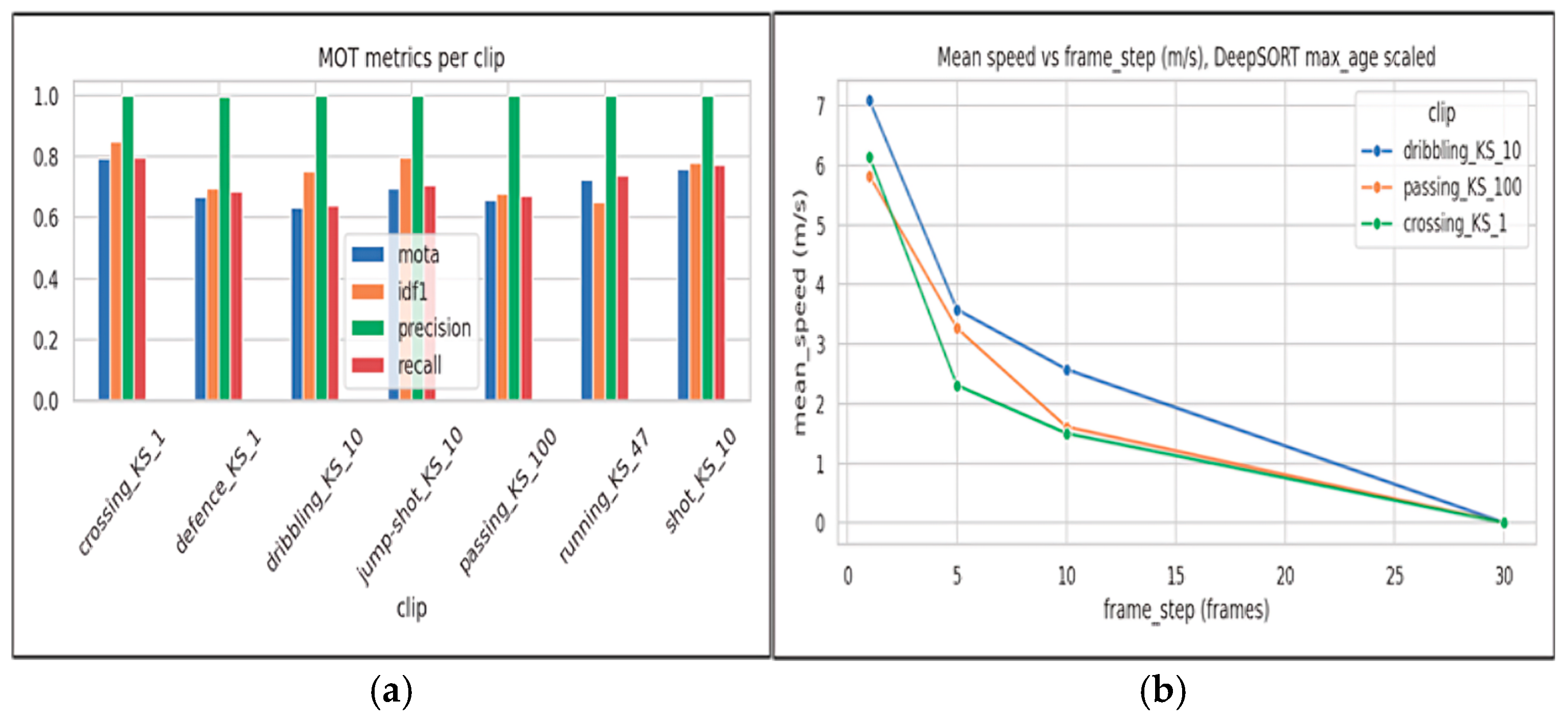
Figure 6.
Example court-density heatmap (normalized) computed from projected trajectories.
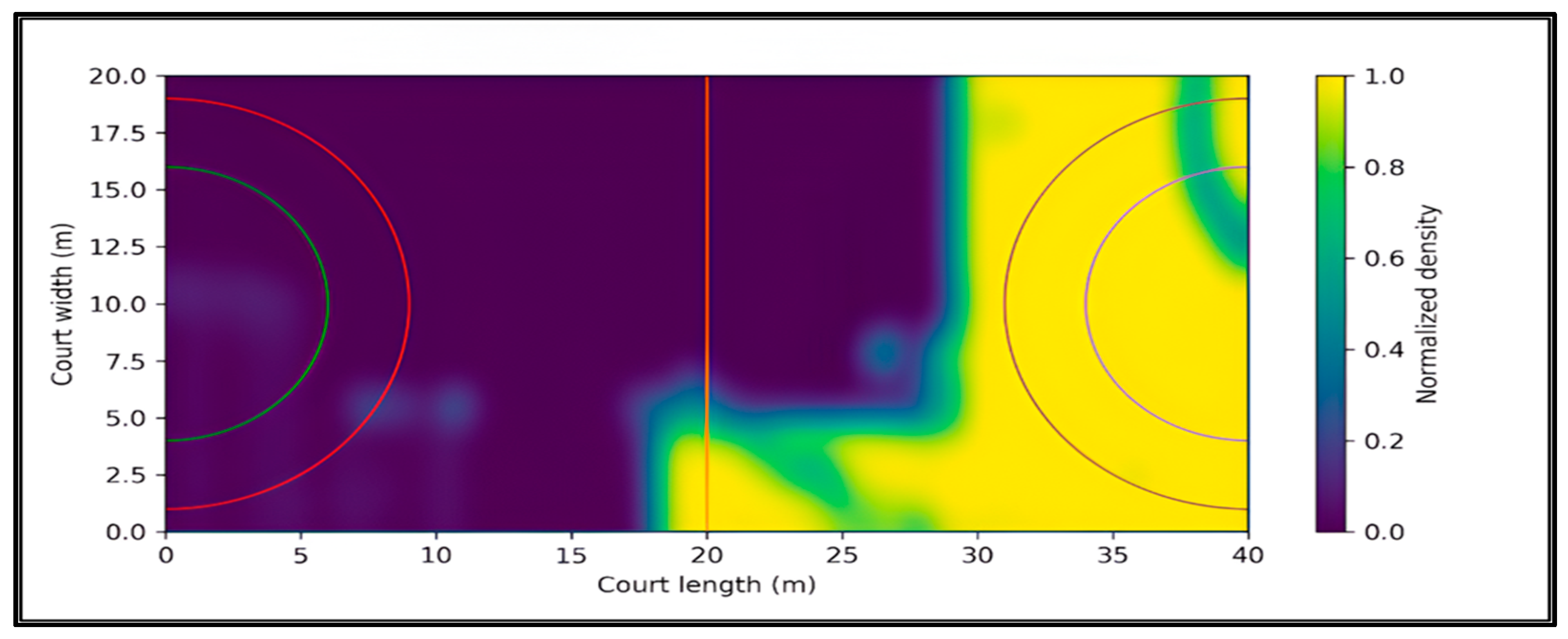
Figure 7.
Confusion matrix for the best-performing Random Forest classifier.
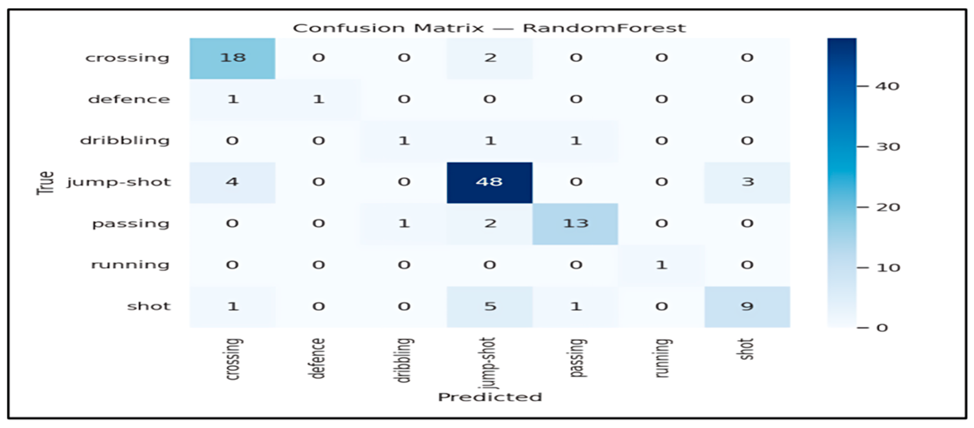
Figure 8.
Feature importance for the Random Forest classifier (trajectory-derived features).
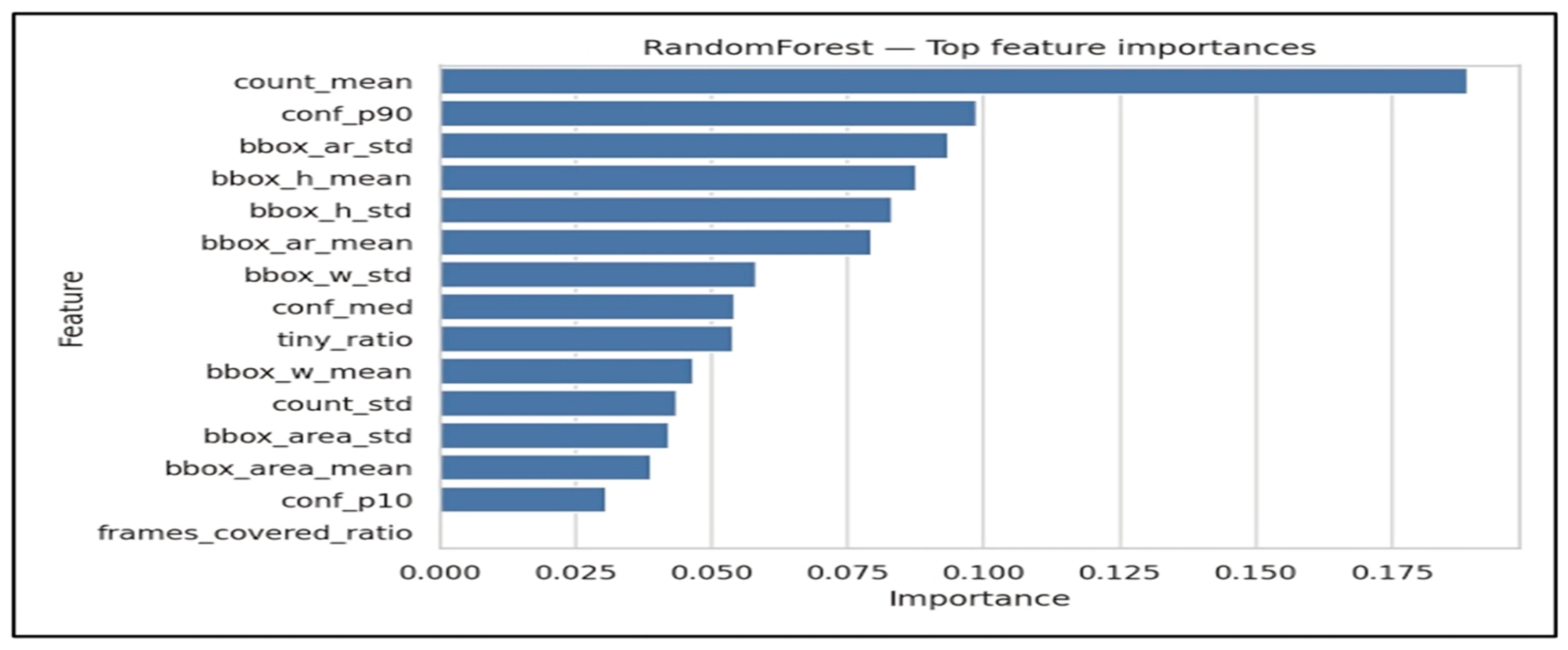

Table 1.
Detection-derived features for scene density, box geometry, and confidence.
| Feature | Short Definition | In Practice | |
|---|---|---|---|
| count_mean |
Mean number of detections per frame. |
Average Crowding Level. |
|
| conf_p90 |
90th percentile of detection confidence scores. |
Confidence of best detections. |
|
| bbox_ar_std |
Std of bounding-box aspect ratio. |
Box Shape Variability (Affected by occlusion/blur). |
|
| bbox_h_mean | Mean bounding-box height. |
Typical target scale in the image (zoom/distance). |
|
| bbox_h_std | Std of bounding-box height |
Stability of target scale over time. |
|
| bbox_ar_mean | Mean bounding-box aspect ratio. |
Typical box shape within the clip. |
|
| bbox_w_std | Std of bounding-box width. |
Variability in box width. |
|
| conf_med |
Median detection confidence. |
Typical detector confidence. |
|
| tiny_ratio | Proportion of tiny boxes. |
Presence of exceedingly small targets. |
|
| bbox_w_mean | Mean bounding-box width. |
Typical target scale in width (zoom/distance). |
|
| count_std | Std of detections per frame. |
How much the number of detections fluctuates across time. |
|
| bbox_area_std | Std of box area. | Variability in overall box size. | |
|
bbox_area_mean |
Mean box area. |
Typical overall box size. |
|
| conf_p10 |
10th percentile of detection confidence scores. |
Strength of the least confident detections. |
|
| frames_covered_ratio |
Fraction of frames with at least one detection. |
Detection coverage over the clip. |
Table 2.
Player detection performance on the evaluation split.
| Metric | Value |
|---|---|
| Precision | 0.896 |
| Recall | 0.768 |
| mAP@0.5 | 0.858 |
| mAP@0.5:0.95 | 0.562 |
Table 3.
Multi-object tracking performance (CLEAR MOT).
| Metric | Value |
|---|---|
| MOTA | 0.71 |
| IDF1 | 0.74 |
| Precision | 1.00 |
| Recall | 0.72 |
Table 4.
Action recognition results using trajectory-derived features.
| Model | Accuracy | Precision | Recall | F1 - Score |
|---|---|---|---|---|
| Random Forest | 0.805 | 0.813 | 0.712 | 0.745 |
| Gradient Boosting | 0.805 | 0.806 | 0.712 | 0.743 |
| Extra Trees | 0.791 | 0.730 | 0.715 | 0.719 |
| XGBoost | 0.761 | 0.687 | 0.703 | 0.693 |
| Logistic Regression | 0.619 | 0.511 | 0.676 | 0.540 |
| Gaussian Naive Bayes | 0.451 | 0.440 | 0.573 | 0.431 |
Disclaimer/Publisher’s Note: The statements, opinions and data contained in all publications are solely those of the individual author(s) and contributor(s) and not of MDPI and/or the editor(s). MDPI and/or the editor(s) disclaim responsibility for any injury to people or property resulting from any ideas, methods, instructions or products referred to in the content. |
© 2026 by the authors. Licensee MDPI, Basel, Switzerland. This article is an open access article distributed under the terms and conditions of the Creative Commons Attribution (CC BY) license (http://creativecommons.org/licenses/by/4.0/).
Copyright: This open access article is published under a Creative Commons CC BY 4.0 license, which permit the free download, distribution, and reuse, provided that the author and preprint are cited in any reuse.


