
Submitted:
20 February 2026
Posted:
25 February 2026
You are already at the latest version
Abstract
This study analyzes the structural roles of economic sectors in Bangladesh using a social accounting matrix exhibiting linkage analysis and simulation. The linkage analysis identifies agriculture, retail trade, transport, and other services as key sectors of the economy. It further shows the simulation of expanding total export shares given to the sectors under different diversification scenarios (foster Vs present) to find out which scenario brings higher output gains. The result from simulation shows that foster scenario generates higher economic gains compared to the other scenario. It further identifies sectors from extensive categories more capable of bringing strong GDP gains while sectors from intensive category except for textiles marginally contributes to GDP and labor earnings in both scenarios. These findings provide empirical support for reconsidering sectoral priorities with intersectoral connection and inform how to promote diversification for inclusive development.
Keywords:
IOT
; linkage
; policy
; diversification
; sector
1. Introduction
Structural change is a natural process in an economy and when positive, can promote economic development, growth, productivity, and higher living standards. It occurs when resources and production shift between economic activities, reorganizing the composition of the economy [1]. Over time, these changes significantly affect economic growth, with some sectors expanding and others contracting [2]. Each sector is important because it contributes uniquely to the economy through production linkages. Such linkages can generate additional economic activities; for example, South Africa’s mining sector developed around its resource endowments [3]. Therefore, structural reforms are often examined as tools for economic adjustment, which are essential for effective policy formulation [4].
Bangladesh has undergone sectoral reforms since independence, achieving steady growth after the 1980s. Although the agricultural sector experienced variable growth, the manufacturing sector became the primary driver of faster economic expansion after 1980. In 2012 agriculture and textile sector becomes responsible for economic growth and higher labor income [5]. But based on 2017 economic data in addition to textiles, real estate services and transport services also became major contributors to the economy [6]. These findings indicate that the economic structure has shifted to rely more on service sectors alongside manufacturing. As the economic growth of service sectors increased, exports from these sectors also increased slowly due to the government supportive policies in the last three decades. However, this shift of diversified export policy is challenging, because previously established policies have primarily supported manufacturing goods [7]. Research found that weak policy reforms and insufficient incentives continued to discourage non-textile exports [8]. So, without structural and institutional reforms, the goals of export policy diversification will remain largely unrealized. In this context, the present research examines how diversified export policy can generate tangible economic benefits through robust sectoral analysis. This paper first identified the key sectors of the economy. Then with simulated alternative scenarios of export diversification this study shows how those sectors contribute to higher GDP.
1.1. Contextual Review of the Issue
Bangladesh will graduate from Least Developed Country (LDC) status in 2026, after which the economy will face trade-related challenges. The country will lose all preferential access designed for LDCs. Some literature identified that graduation from LDC status can harm total exports by 4-8% [9,10]. On the contrary a study was conducted using LDC graduating countries from 52 regions of the world using Global Trade Analysis Project (GTAP) model 2014, which found that withdrawal of preferential market access from LDCs does not necessarily translate into substantial economic losses for countries with diversified export bases, even they can improve welfare by attracting more investment through Free Trade Agreements (FTAs). [11]. Taking reference from the above and due to the high dependency on textile sector for export, Bangladesh also being suggested to diversify its export mix with active FTAs negotiation to major trade partners. In line with the Perspective plan 2041 with high priority objective there is a gradual increase in export diversification. Figure 1 shows the progress of export composition to provide a clear view of the pattern of diversification unfolded in the past 10 years. This figure shows textile
exports accounting for most of the total export earnings [12]. Although the other exports were smaller, they experienced periods of moderate growth until 2020. Following this year a 2.4% decline in exports with rebounding textile exports questioned the stability of diversification policy.
The decline of other exports or raising of textile exports in 2022 is accelerated by the post-pandemic shift in global sourcing behavior associated with the China-plus-one (CP1) strategy adopted by major North American buyers. After the COVID-19 disruptions, export orders have moved from China toward alternative south Asian suppliers. Due to the above strategy Bangladesh experienced an increasing share in textile exports by 9.75% to the US market [13,14,15].
1.2. Rationale for the Export-Diversification Simulation Design
To sustain post LDC graduation challenges the country is successfully advancing negotiations with its major trading partners. It is proved that countries having multiple FTAs can gain an additional export boost from network effects [16]. So, It can be assumed that future export demand in Bangladesh is likely to rise sharply once these agreements come into force. There are some empirical evidence that due to raising number of trade agreements total exports grows by 5 to 11% yearly [17,18]. To estimate how this higher export affects the economy, this study uses the findings from Foster who showed that Preferential Trade Agreements (PTAs) increases exports of small exporters by 11-13% [19]. It is further estimated that trade with small partners raises exports mainly through the intensive margin (selling more of the same products), while trade with large partners raises exports mostly through the extensive margin (adding new export products).
Considering this economy as a small exporter, this study simulates an overall 11 percent export-demand shock and splits it into two different scenarios, i.e. foster scenario and present scenario. To conduct the above scenarios, sectors that contribute more than 1 percent to total exports are considered as intensive sectors while others as extensive (needs special attention to grow their export share). Under foster scenario higher shock is given to extensive sectors while lower shock is given to intensive sectors following his estimation. This scenario assumption is based on the idea that FTAs will primarily open opportunities for new products from low exporting sectors. In present scenario the full shock is distributed to intensive sectors only while keeping the extensive sectors constant to illustrate the limitation of current export diversification bias which is highly dominated by a few intensive sectors.
After comparison this study showed which type of diversification can generate higher output. The result guide policymakers on which sectors should be prioritized first and how to design a sustainable and more diversified export mix.
The following section outlines the methodological framework, including data sources, the construction and balancing of SAMs using the Simulation for Social Indicators and Poverty using SAM (SIMSIP SAM) tool, the analytical methods for linkage analyses, and the structure and purpose of the simulation scenarios. Section 3 presents the results of the linkage analysis to assess the effectiveness of export shock interventions. Section 4 concludes with a summary of the empirical results and their policy implications.
2. Materials and Methods
This research uses a two-stage analytical methodology to examine the simulation under different scenarios. The first step is to convert IOT into SAM for the database. Based on this database, we then proceed to linkage analyses and simulate the export scenarios based on the GDP and the labor income. Before presenting the model and simulation, we describe the data framework.
2.1. Database
This analysis used the SAM database. To examine the broader effects of policy actions, the SAM provided a strong economic model foundation because it measures interdependence among sectors, variables, and institutions beyond the IOT [20,21]. The SAM for this analysis was derived from the IOT published by the Economic Research and Development Impact Department (ERDI) of the Asian Development Bank (ADB) [22]. Sectoral labor income is calculated by allocating total value added across sectors using labor composition shares derived from the Labor Force Survey (LFS) of 2017 and 2022, which are incorporated into the Social Accounting Matrix as fixed allocation coefficients [23]. This approach assumes fixed labor shares by sector and does not account for within-sector wage heterogeneity. The SAM was divided into endogenous accounts, including labor, capital, and households, and exogenous accounts, comprising government, capital, and foreign sectors [24].
2.2. Construction Steps of SAM from IO
This study applies to a comprehensive SAM framework by expanding the IOT. The IOT consists of 34 productive sectors. The SAM includes institutional sectors and factor accounts in addition to the 34 sectors to represent the entire circular flow of revenue and convert it into a closed, balanced matrix suitable for analysis [25]. Figure 2 presents the complete construction process from IOT to SAM. The process begins with the disaggregation of the IO value-added account.
This disaggregation includes labor compensation, representing employee wages and salaries, and capital income, which consists of gross operating surplus (GOS) and land rents, following national accounts conventions. Labor income for different sectors is calculated using value-added data from IO and labor share data from LFS. Capital income is derived residually by subtracting labor earnings from total value-added for each sector. To construct and calibrate the SAM used in this study, we used the SIMSIP SAM software developed by the World Bank [26]. In this study, SIMSIP SAM was straightforward to adopt for balancing the SAM. The program offers two algorithms for balancing matrices: the RAS technique and the cross-entropy approach. To preserve the original matrix structure in line with national accounting statistics and maintain valid sectoral data, this study selected the RAS technique over the cross-entropy approach.
2.3. Linkage Analyses
This study assesses intersectoral linkages through identifying key sectors. Traditionally, sectoral interdependence has been measured with the input–output (IO) model.
2.3.1. Backward Linkage
Rasmussen introduced backward linkages (BL) to capture the stimulus a sector receives from others through intermediate demand [27], while Augustinovics (1970) developed forward linkages (FL) to represent the extent to which a sector transmits effects to others through its supply of intermediate inputs [28]. This study extends the BL and FL approaches by using a SAM, rather than a conventional IOT, as the analytical database. Following the basic IO relationship, the SAM model is represented as follows:
where E is the vector of endogenous accounts, Ex is the vector of exogenous accounts, and denotes the SAM multiplier matrix, which is conceptually analogous to the Leontief inverse in the IO model [29]. We denote the following SAM multiplier matrix as At, which is later used for the reference of column sum vector Aj to calculate BL.
where I is an identity matrix of size n and S is the average tendency matrix (the SAM coefficient matrix) of expenditure between the different endogenous accounts. The following normalized expression of BL was obtained according to Rasmussen.
(I-S)-1 = At
Column sum vector is calculated by (summing all elements aij from a given column of each sector j that belongs to the (At) equation 2). Here, j ranges from 1 to n (n = 34) and V is the global intensity, a scalar value of the total sum of all elements in the associated inverse matrix for the total economic activity [30]. If the BL is above hundred, a one-unit change in the final demand of sector j will generate growth above the average on the global activity of the economy.
2.3.2. Forward Linkage
FL are measured to assess the extent to which a sector’s output is used as input by other sectors in their production processes. The traditional method, based on Rasmussen approach of summing the rows of the Leontief inverse matrix (I -A)-1, has been criticized for its symmetry with BL and its failure to reflect the supply-driven nature of sectoral flows. To address these methodological issues, this study applies the approach proposed by Augustinovics , which calculates FL using the Ghosh inverse matrix from the supply-driven input–output model. To maintain the supply-driven perspective of SAM within the Ghosh framework, we used the corresponding inverse matrix equation Gt = (I - Bs)-1, where Bs is the matrix of output coefficients. Here, the row sum vector Bi is calculated by summing all elements bij within each row of the inverse matrix Gt. Each element bij represents the ratio of the output from sector i that is used as an input into sector j, scaled by the total output of sector i. Here, the term sector encompasses not only productive sectors, but also value-added and institutional factors (e.g., labor, capital, households), reflecting the broader distribution of production and income flows across the entire economic system. This study then calculated FL using the following formula:
The global intensity V is calculated as . If the forward linkage is above hundred, a one-unit change in the output of a given sector on average induces more than one unit of demand across the downstream sectors that use its output as an intermediate input.
2.4. Export Policy Simulation
Linkage analysis reveals the structural interdependencies within an economy by providing a static representation of the economic system under equilibrium conditions. In contrast, simulation analysis introduces dynamic elements by examining how the economy responds to exogenous shock. Consequently, when interpreting simulation results, it is important to reference previous linkage analyses to understand the underlying transmission mechanisms and relate policy scenarios to the actual structure and dynamics of the economy.
To template the intensive and extensive sectors of export diversification, this study assumes the sectors with more than 1 percent of total export value are defined as intensive sectors, meaning they already have an established export base, and their growth is expected to come mainly from expanding existing product lines (the intensive margin). Textile, leather, food, manufacturing, post & telecommunication, renting of M&Eq and public administration are defined as intensive sectors while the rest is extensive sectors in this study.
Consistent with foster estimation, 11 percent shock is allocated as 7 percent to extensive sectors and 4 percent to intensive sectors. In designing the present scenario, we assume the extensive sectors export will not expand during the shock and shock is distributed only across 7 intensive sectors. Although the sectoral distribution is given differently but the aggregated total export value under two scenarios remains same for the basis of comparison.
2.4.1. Foster Diversification Scenario
This scenario, the total targeted export increase (11%) is allocated according to Foster’s extensive–intensive margin decomposition: 7% to extensive sectors and 4% to intensive sectors. This scenario reflects the empirical pattern that small exporters trading with higher product margin experience predominantly export growth. For each sector n, the new export value under the scenario is calculated as:
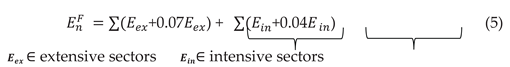
= export value of sector n in the SAM, export value of sectors under extensive category, export value of sectors under intensive category. The difference is then applied as a shock to the export component of final demand vector in SAM by
2.4.2. Present Diversification Scenario
The Scenario assumes that only intensive sectors are targeted to meet the entire increase in export value, while extensive sector exports remain fixed at their 2022 levels. For this scenario total export value of intensive sector is calculated as:
ET= Total export value SAM. The incremental change then calculated by following equation 6. The export value under different diversification is listed in Table 1.
3. Result Interpretation: Linkage Analysis and Simulation-based Scenario Analysis
This section presents the main findings of this research. It describes the integration of insights from linkage analyses and simulations.
3.1. Linkage Analyses of Top Sectors
The research identifies the sectors with the strongest economic effects and the greatest propagation of activity through upstream and downstream production chains. Based on the linkage formula, agriculture (1), retail trade (21), transport (23), and other service (34) sectors were identified as key sectors, each scoring above 100% for both BL and FL. Although these key sectors contributed relatively little to direct export shares, export simulations in the following section showed that they were significantly affected because of their strong backward and forward linkages. This finding demonstrates the importance of linkage analyses of how sectors with minor direct export shares can still have a substantial influence on GDP and labor income through their ripple effects.
The following Figure 3 reveals the leading sectors in the economy. The highest peaks indicate the sectors that are strongly connected with both BL and FL across the economy. Investing in them can create the largest economy-wide ripple effects. Agriculture serves the core backbone of the economy with the highest peak. Along with agriculture other service, textile, retail trade, inland transport sectors etc. also served as the effective stimulus channels interacting to other sectors of the economy. On the other hand rubber, machinery, coke & refined petroleum have the lower interacting power as they found in the marginal place in the ascending order . This chart also shows the importance of intersectoral relationships being the most impact arise from the interaction of agriculture sector with sale, maintenance, and repair of motor vehicles and motorcycles; retail sale of fuel sector. Intersectoral relationship with less economic impact corresponds to the coke and refined petroleum sector with machinery sector.
Table 2 presents the top six sectors by backward and forward linkage scores. Agriculture contributed the largest share to GDP among the selected sectors (12.2%), indicating its continued economic importance. However, its export share was very low (0.69%) relative to its size, and it was highly dependent on imports (9.20%) (see Appendix A2 for detailed export and import data). Agriculture accounted for exceptionally high FL score (187.63) indicating the raw materials and industrial feedstock from agriculture sector were used extensively by other sectors. In contrast, the sector had limited BL, reflecting weaker demand for intermediate inputs from other domestic sectors because of low input use and small-holder-based production systems.
Previous studies primarily found manufacturing sectors are important for economic growth [31]; however, this research identifies service-oriented sectors, such as retail trade (21), inland transport (23), and other service (34), as structurally significant. Retail trade (21) is ranked second among key sectors in terms of its contribution to total GDP of 9.56%. Because of its strong BL with other industries, growth in retail trade (21) can increase output and profit in other sectors. Its high FL (119.74) indicates that retail trade (21) functions as a distribution channel supporting household consumption and downstream economic activity. Given its low export share and strong inter-industry linkages, retail trade (21) is a strong internal driver of demand-driven growth.
According to BSIC, the other service (34) sector specifically includes activities of NGOs, non-profit organizations, international organizations, and undifferentiated goods and services produced by households for their own use [32]. These activities play a crucial role in supporting key sectors such as agriculture (1), textile (4), education (32), and transport (23) through funding, training, and services. Rural development, poverty alleviation, and skill enhancement in downstream sectors have been enhanced by the indirect contributions of this sector, as its FL provides greater value than its BL.
The transport sector (23) is a key strategic sector in the economy because of its strong linkages, supporting downstream industries such as agriculture, manufacturing, and retail, and its significant dependence on upstream sectors for fuel supply, vehicle sales and repairs, and financial services.
3.2. Sectoral Impact of Scenarios on GDP and Labor Income
This section presents the simulation to examine interindustry connections under different scenarios. The two scenarios applied an identical total export expansion (Tk 55,344.33 million) but distribute it differently across sectors. The foster scenario shifts a larger share of the shock toward extensive sectors whereas the other scenario is followed by the intensive sectors. Table 3 shows the foster scenario brings higher gains to the economy compared to the current export mix. Our result is in line with the findings of diversification literature which proves higher economic growth can be obtained through extensive margin having trade with new product [33].
Within the sectoral results, extensive sectors produce stronger GDP gains. These sectors have high potential to contribute to national output when export opportunities expand as they introduce new activities, new input, and new production links into the economy. Specifically sectors identified as key sectors from previous linkage analyses perform better in simulation compare to the high exporting sectors. All those sectors have a very low export share specially retail trade and transport service with zero export. This two sectors generate substantial GDP and labor income effects even with zero export shock. Although Bangladesh exports transport equipment but there are no records for exporting transport services. International evidence shows that developing countries can raise their export revenue by finding and removing the rules that restrict service trade, and by allowing workers to move where needed, so the services inside transport can be sold more easily in foreign markets [34]. This widens the economic base and creates broader value-added effects.
On the other hand, intensive sectors are already exporting heavily, additional export demand tends to produce smaller incremental value-added, as most gains are absorbed by existing capital-intensive or import-intensive production structures.
The (27) post and telecommunication add only marginal gains to GDP and labor earnings in present scenario. Interestingly the (30) renting of M & Eq exhibits lower GDP and labor-income in present scenario where the shock is given higher compared to the other scenario. Taking reference from previous linkage analyses the BL of this above two sector is high but their FL is very low. This asymmetric linkage structure severely constrains the downstream propagation or returns of those sectors.
4. Discussion and Policy Implications
The findings of this study challenge the current diversification strategy. Our simulations show that although extensive sectors account for only a small share of current exports, applying even a slightly larger shock to them generates prominently stronger economic gains compared to intensive sectors, indicating that these sectors should receive greater strategic attention in the design of a future export mix. In contrast, most intensive sectors, aside from textiles, exhibit weak backward and forward linkages, which restrict their ability to fully transmit the gains from export expansion throughout the economy. This structural bottleneck explains why increases in export demand do not translate into substantial domestic value-added or labor earnings in these sectors. Therefore, our results highlight the need to rethink the diversification approach by incorporating a more balanced combination of extensive and intensive sectors. In particular, (1) agriculture, (34) other service, (21) retail trade and (23) inland transport although having lower export shares but can generate higher returns to the economy. The (27) post & telecommunication and (30) renting of machinery and equipment sectors should be prioritized for policy support to strengthen their FL linkages. Enhancing these structural connections would enable them to absorb larger export shocks and contribute more meaningfully to GDP and employment. Overall, the study suggests that a diversified strategy built on the extensive–intensive concept offers a more effective pathway for generating sustainable income and broad-based economic gains.
Author Contributions
The conceptualization of this study was carried out by J M and H T. The methodology, investigation, resources, data curation and original draft preparation were undertaken by J M. Formal analysis was conducted by C A M. The review and editing of the manuscript were completed by C A M and H T. Supervision was provided by H T and C A M and funding acquisition was secured by H T. All authors have read and agreed to the published version of the manuscript.
Funding
This research was supported by the Sophia University SPRING Project, which is funded by the Japan Science and Technology Agency (JST).
Data Availability Statement
Data supporting the reported results are available from the author upon reasonable request.
Acknowledgments
The author gratefully acknowledges Professor Akira Kohsaka and Assistant Professor Nguyen Vuong for their insightful and constructive comments on an earlier version of this paper presented at the 20th East Asia Economic Association International Conference. Their valuable feedback substantially improved the analytical clarity and overall quality of the study.
Conflicts of Interest
The authors declare no conflicts of interest. The funders had no role in the design of the study; in the collection, analyses, or interpretation of data; in the writing of the manuscript; or in the decision to publish the results.
Abbreviations
The following abbreviations are used in this manuscript:
| IOT | Input–Output Table |
| SAM | Social Accounting Matrix |
| ADB | Asian Development Bank |
| P&T | Post and telecommunication Technology |
| M & Eq | Machinery and Equipment |
| LDC | Least Developed Country |
| FTA | Free Trade Agreements |
| PTA | Preferential Trade Agreements |
| CP1 | Chaina Plus one |
| SIMSIPSAM | Social Impact Simulation for Social Accounting Matrix |
| ERDI | Economic Research and Development Impact Department |
| LFS | Labor Force Survey |
| GOS | Gross Operating Surplus |
| RAS | Bi-proportional Matrix Balancing Method |
Appendix

Table A1.
Backward and Forward linkage of 34 sectors. The full table of table no. 2 is given below.
| Backward linkages | % | Forward linkages | % |
| Sale of motor vehicles and motorcycles | 114.58 | Agriculture, hunting, forestry, and fishing | 187.63 |
| Retail trade, except for motor vehicles; | 111.79 | Other services | 144.14 |
| Other nonmetallic minerals | 111.76 | Textiles and textile products | 119.83 |
| Real estate activities | 110.92 | Retail trade, except for motor vehicles; | 119.74 |
| Financial intermediation | 110.48 | Inland transport | 114.08 |
| Other services | 110.27 | Food, beverages, and tobacco | 99.27 |
| Mining and quarrying | 109.28 | Real estate activities | 79.99 |
| Education | 109.26 | Financial intermediation | 60.11 |
| Public administration and defense | 108.86 | Construction | 54.83 |
| Post and telecommunications | 108.74 | Basic metals and fabricated metals | 49.77 |
| Electrical and optical equipment | 108.66 | Hotels and restaurants | 44.67 |
| Renting of M&Eq and other business activities | 108.23 | Other nonmetallic minerals | 43.86 |
| Wood and products of wood and cork | 107.06 | Health and social work | 40.89 |
| Other transport activities | 106.81 | Manufacturing, nec; recycling | 39.52 |
| Leather, leather products, and footwear | 106.67 | Wholesale & commission trade | 38.82 |
| Transport equipment | 105.78 | Education | 37.87 |
| Water transport | 105.77 | Electricity, gas, and water supply | 35.57 |
| Wholesale & commission trade | 105.09 | Leather, leather products, and footwear | 30.41 |
| Inland transport | 104.99 | Renting of M&Eq | 29.69 |
| Manufacturing, nec; recycling | 103.75 | Mining and quarrying | 28.78 |
| Electricity, gas, and water supply | 101.87 | Sale of motor vehicles and motorcycles | 23.38 |
| Agriculture, hunting, forestry, and fishing | 101.57 | Chemicals and chemical products | 23.10 |
| Hotels and restaurants | 101.28 | Public administration and defense | 22.14 |
| Construction | 98.66 | Wood and products of wood and cork | 21.98 |
| Chemicals and chemical products | 98.37 | Other transport activities | 20.13 |
| Rubber and plastics | 94.85 | Transport equipment | 19.98 |
| Food, beverages, and tobacco | 94.03 | Water transport | 19.77 |
| Basic metals and fabricated metals | 93.30 | Pulp, paper, paper products, | 19.72 |
| Air transport | 92.78 | Post and telecommunications | 18.20 |
| Health and social work | 89.32 | Air transport | 15.06 |
| Textiles and textile products | 89.13 | Rubber and plastics | 14.67 |
| Pulp, paper, paper products, printing, | 80.56 | Machinery, nec | 13.20 |
| Machinery, nec | 64.85 | Electrical and optical equipment | 13.14 |
| Coke, refined petroleum, and nuclear fuel | 40.17 | Coke, refined petroleum, and nuclear fuel | 12.82 |
Table A2.
GDP, Export and Import share based on 2022 SAM.
| Sl | Sectors | Export % | Import % | GDP % |
| 1 | Agriculture, hunting, forestry, and fishing | 0.69 | 9.20 | 12.21 |
| 2 | Mining and quarrying | 0.01 | 0.28 | 1.59 |
| 3 | Food, beverages, and tobacco | 1.97 | 8.02 | 2.08 |
| 4 | Textiles and textile products | 75.21 | 27.17 | 7.07 |
| 5 | Leather, leather products, and footwear | 3.87 | 0.71 | 0.82 |
| 6 | Wood and products of wood and cork | 0.06 | 0.34 | 0.42 |
| 7 | Pulp, paper, paper products, printing, and publishing | 0.11 | 1.03 | 0.22 |
| 8 | Coke, refined petroleum, and nuclear fuel | 0.00 | 0.01 | 0.00 |
| 9 | Chemicals and chemical products | 0.67 | 0.77 | 0.52 |
| 10 | Rubber and plastics | 0.14 | 0.34 | 0.13 |
| 11 | Other nonmetallic minerals | 0.16 | 0.80 | 3.11 |
| 12 | Basic metals and fabricated metals | 0.16 | 7.54 | 1.35 |
| 13 | Machinery, nec | 0.11 | 0.35 | 0.05 |
| 14 | Electrical and optical equipment | 0.31 | 0.05 | 0.08 |
| 15 | Transport equipment | 0.39 | 1.11 | 2.00 |
| 16 | Manufacturing, nec; recycling | 1.74 | 2.87 | 2.41 |
| 17 | Electricity, gas, and water supply | 0.00 | 1.51 | 1.35 |
| 18 | Construction | 0.86 | 19.94 | 8.99 |
| 19 | Sale of motor vehicles and retail sale of fuel | 0.00 | 0.03 | 0.84 |
| 20 | Wholesale trade | 0.00 | 1.12 | 2.93 |
| 21 | Retail trade | 0.00 | 0.42 | 9.56 |
| 22 | Hotels and restaurants | 0.73 | 2.16 | 1.01 |
| 23 | Inland transport | 0.00 | 4.19 | 7.16 |
| 24 | Water transport | 0.10 | 0.25 | 0.44 |
| 25 | Air transport | 0.42 | 0.30 | 0.05 |
| 26 | Other transport activities | 0.00 | 0.17 | 0.43 |
| 27 | Post and telecommunications | 6.84 | 0.34 | 1.07 |
| 28 | Financial intermediation | 0.57 | 0.84 | 4.16 |
| 29 | Real estate activities | 0.00 | 0.19 | 5.92 |
| 30 | Renting of M&Eq and other business activities | 3.69 | 0.43 | 1.61 |
| 31 | Public administration and defense; compulsory social security | 1.06 | 1.03 | 3.97 |
| 32 | Education | 0.00 | 0.60 | 3.16 |
| 33 | Health and social work | 0.00 | 4.11 | 2.56 |
| 34 | Other community, social, and personal services | 0.11 | 1.76 | 10.73 |
References
- Constantine, C. Economic Structures, Institutions, and Economic Performance. Journal of Economic Structures 2017, 6, 1–16. [Google Scholar] [CrossRef]
- Krüger, J.J. Productivity and Structural Change: A Review of Literature. Journal of Economic Surveys 2008, 22, 330–363. [Google Scholar] [CrossRef]
- Schwank, O.; Wild, M. Testing for Linkages in Sectoral Development: A SVAR Approach to South Africa. In Proceedings of the 5th International Conference on Developments in Economic Theory and Policy, Bilbao, Spain, 9–10 July 2008. [Google Scholar]
- Li, R.; Wang, Q.; Liu, Y.; Jiang, R. Per-Capita Carbon Emissions in 147 Countries: The Effect of Economic, Energy, Social, and Trade Structural Changes. Sustainable Production and Consumption 2021, 27, 1149–1164. [Google Scholar] [CrossRef]
- Khondker, B.H. Backward and Forward Linkages in the Bangladesh Economy: Application of the Social Accounting Matrix Framework. In South Asia Economic and Policy Studies; Palgrave Macmillan: Singapore, 2018; pp. 171–187. [Google Scholar] [CrossRef]
- Huq, M.T.; Ichihashi, M. Prospective Accelerating Sectors to Attain Sustainable Development in the Bangladesh Economy: Findings from a Sectoral Approach Using Input-Output Analysis. Sustainability 2023, 15, 2651. [Google Scholar] [CrossRef]
- Ginting, E.; Razzaque, M.A.; Hasan, R. Export Diversification in Bangladesh: Overcoming Policy Impediments. Asian Economic Policy Review 2024. [Google Scholar] [CrossRef]
- Razzaque, M. A. Revitalizing Bangladesh's export trade: Policy issues for growth acceleration and diversification. 2017. [Google Scholar] [CrossRef]
- Rashid, H. Bangladesh’s Transition from Least-Developed-Country Status: Navigating Export Challenges in a New Era. Asian Journal of Economics, Business and Accounting 2025, 25, 74–91. [Google Scholar] [CrossRef]
- Hussain, Z.; Rizwan, N. Bangladesh Development Update; World Bank: Washington, DC, USA, 2013; Available online: http://documents.worldbank.org/curated/en/944031468212071200.
- Valenzuela, E.; Gunasekera, D. Least developed countries’ graduation: effects of preferential market access loss and investment benefits. SSRN Electronic Journal 2020. [Google Scholar] [CrossRef]
- Asian Development Bank. (2018). Bangladesh Input–Output Tables and Analysis, 2000–2022 (Updated 15 July 2023). Economics Research and Development Impact Department (ERDI). Asian Development Bank. https://data.adb.org .
- New age. Bangladesh’s RMG exports to US cross $10b in 2022, 2023. Available online: https://www.newagebd.net/article/193941/bangladeshs-rmg-exports-to-us-cross-10b-in-2022#:~:text=Readymade%20garment%20exports%20from%20Bangladesh%20to%20the,cent%20in%202021%2C%20the%20OTEXA%20data%20showed.
- Rahaman, M.; Pranta, A.; Chandrow, O.; Das, N.; Khatun, M.; Arafat, M.; Sami, W. COVID-19 Pandemic and the Future of China-Plus-One Strategy in Apparel Trade: A Critical Analysis from Bangladesh-Vietnam Point of View. Open Journal of Business and Management 2021, 9, 2183–2196. [Google Scholar] [CrossRef]
- Ali, M.; Qun, W.; Hossain, M. E. Revealed Comparative Advantage of Textile and Clothing Industry of Bangladesh in the North American Market. Journal of Business Management and Economic Research 2019, 3(1), 28–42. [Google Scholar] [CrossRef]
- Hur, Jung, Joseph D. Alba, and Donghyun Park. “Effects of Hub-and-Spoke Free Trade Agreements on Trade: A Panel Data Analysis.” World Development 38, no. 8 (2010): 1105–1113.
- Hannan, S. Ahmed.The Impact of Trade Agreements: New Approach, New Insights. IMF Working Papers 2016/117. Washington, DC: International Monetary Fund. [CrossRef]
- Baier, Scott L., and Jeffrey H. Bergstrand. Do Free Trade Agreements Actually Increase Members’ International Trade? Journal of International Economics, 2006. 71 (1): 72–95. [CrossRef]
- Foster, N.; Poeschl, J.; Stehrer, R. The impact of Preferential Trade Agreements on the margins of international trade. Economic Systems 2010, 35(1), 84–97. [Google Scholar] [CrossRef]
- Cardenete, M.A.; Sancho, F. Missing Links in Key Sector Analysis. Economic Systems Research 2006, 18, 319–325. [Google Scholar] [CrossRef]
- Scandizzo, P.L.; Ferrarese, C. Social Accounting Matrix: A New Estimation Methodology. Journal of Policy Modeling 2015, 37, 14–34. [Google Scholar] [CrossRef]
- ERDI. Bangladesh: Input-output economic indicators (national input-output tables). Asian Development Bank, 2023. [Google Scholar]
- Bangladesh Bureau of Statistics (BBS). Bangladesh labor force survey 2022. International Labor Organization Survey Catalog. Reference ID: bgd_2022_lfs_v01_m_ilo_var.
- Villegas, P.; Del Carmen Delgado, M.; Cardenete, M.A. The Economic Impact of a Tourist Tax in Andalusia Examined through a Price-Effect Model. Applied Economics Letters 2022, 31, 96–101. [Google Scholar] [CrossRef]
- Marca, M.L.; Jiang, X. From IO and Supply-and-Use to Social Accounting Matrix Analysis. In How to Measure and Model Social and Employment Outcomes of Climate and Sustainable Development Policies; International Labour Organization: Geneva, Switzerland, 2017; pp. 157–202. [Google Scholar]
- Parra, J.C.; Wodon, Q. A Tool for the Analysis of Input-Output Tables and Social Accounting Matrices; World Bank: Washington, DC, USA, 2009. [Google Scholar]
- Rasmussen, P. Studies in Inter-Sectorial Relations; Einar Harks: Copenhagen, Denmark, 1956. [Google Scholar]
- Augustinovics, M. Methods of International and Intertemporal Comparison of Structure. In Contributions to Input-Output Analysis; Carter, A.P., Bródy, A., Eds.; North-Holland: Amsterdam, The Netherlands, 1970; pp. 249–269. [Google Scholar]
- Leontief, W. The Dynamic Inverse. In Contributions to Input-Output Analysis; Carter, A.P., Brody, A., Eds.; North-Holland: Amsterdam, The Netherlands, 1970; Volume 1, pp. 17–46. [Google Scholar]
- Guilhoto, J.J.M.; Sonis, M.; Hewings, G.J. Multiplier Product Matrix Analysis for Interregional Input-Output Systems: An Application to the Brazilian Economy. MPRA Paper No. 54671, University Library of Munich, Germany, 1999. Available online: https://mpra.ub.uni-muenchen.de/54671/ .
- Manik, M.H. Movement of the Economy of Bangladesh with Its Sector-Wise Contribution and Growth Rate. Journal of Production Operations Management and Economics 2023, 32, 1–8. [Google Scholar] [CrossRef]
- BSIC. Bangladesh Standard Industrial Classification; Bangladesh Standard Industrial Classification: Dhaka, Bangladesh, 2020. [Google Scholar]
- Rondeau, Fabien and Nolwenn Roudaut. “What Diversification of Trade Matters for Economic Growth of Developing Countries.” Economics Bulletin 34 , 2014: 1485-1497.
- Suryavanshi, P. Trade in services and economic development. SSARSC International Journal of Geo Science and Geo Informatics 2020, 1, 1–8. [Google Scholar] [CrossRef]
Figure 1.
Export composition 2015-22.
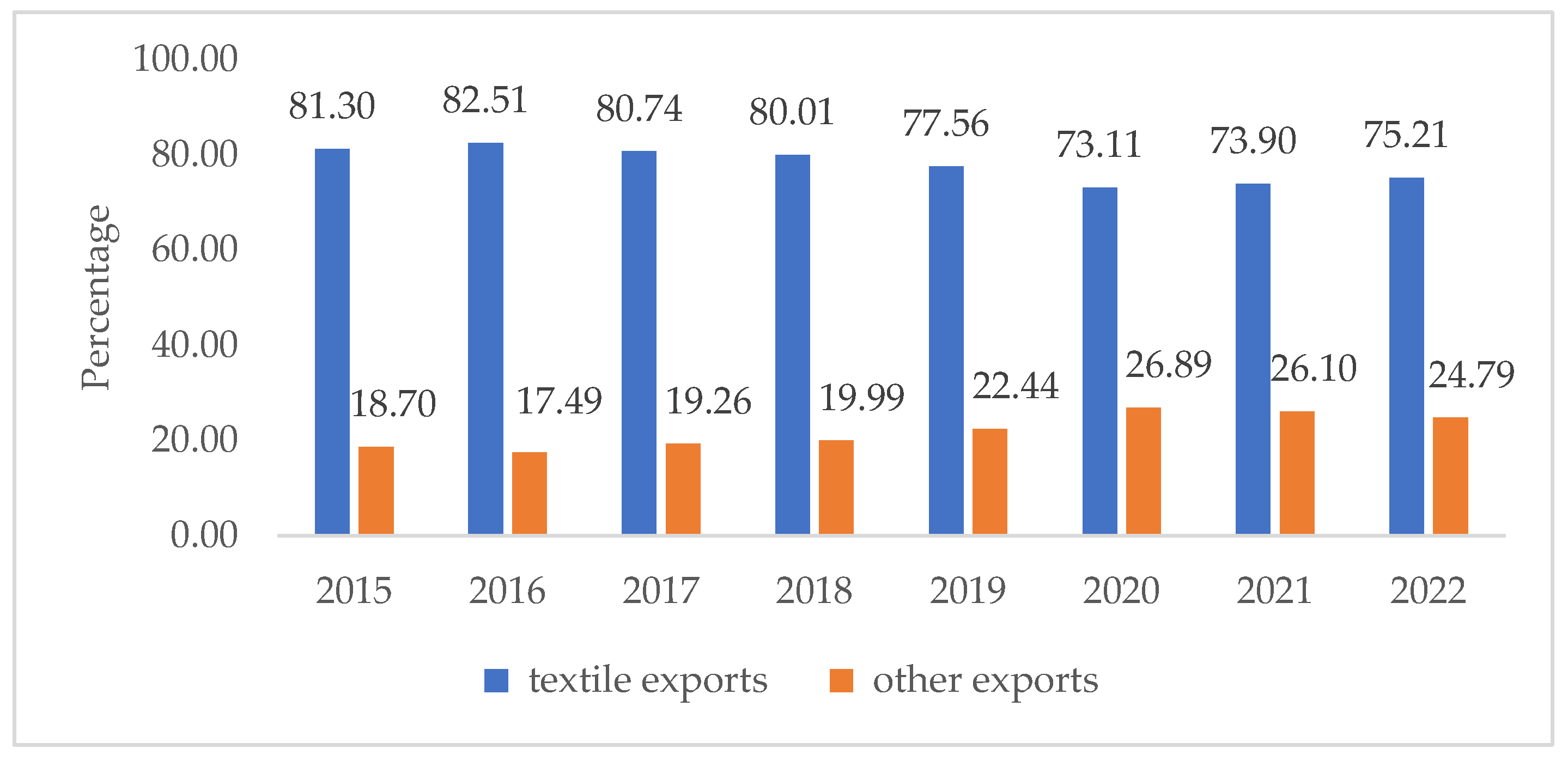
Figure 2.
Steps followed in the construction of Bangladesh SAM 2022.
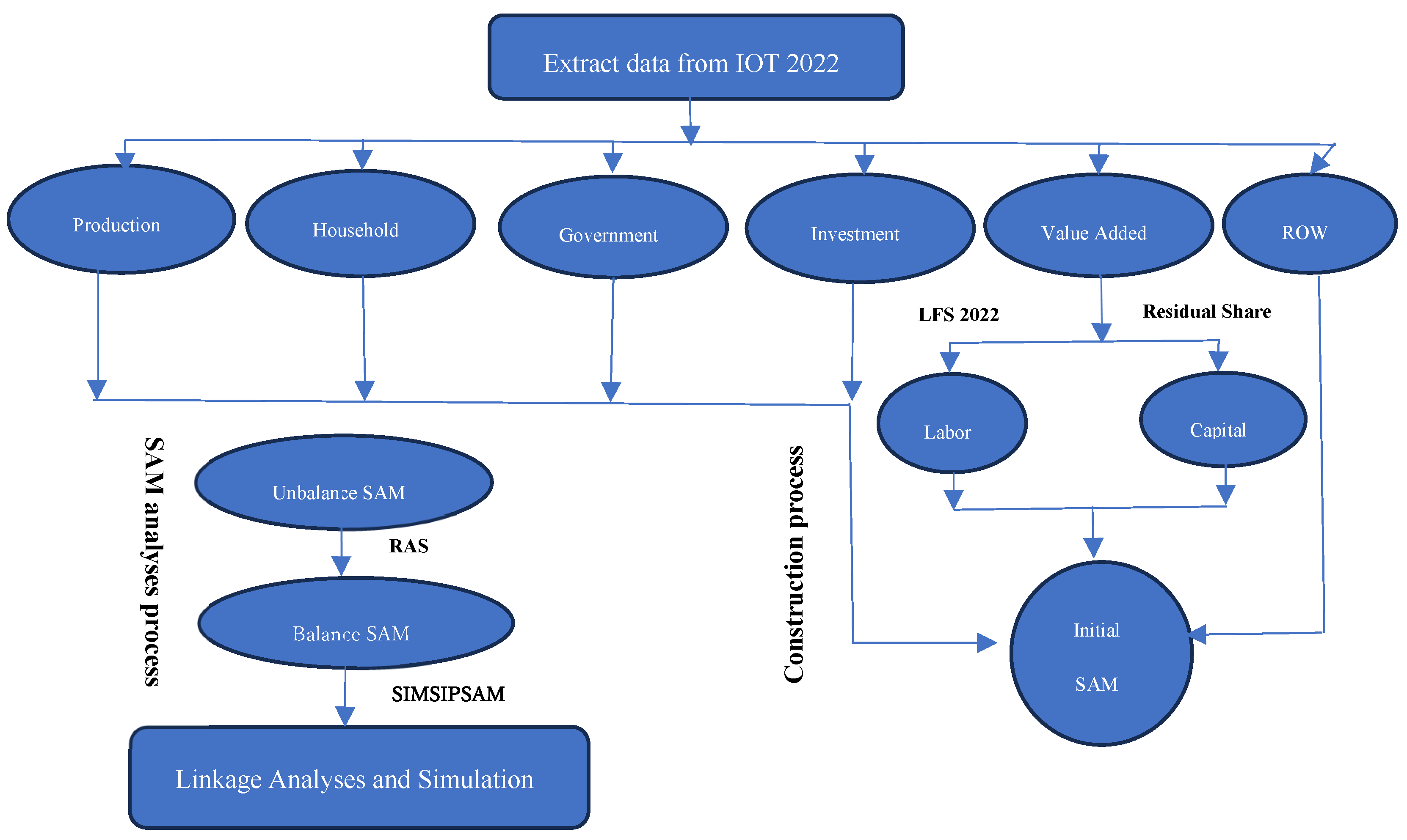
Figure 3.
Economic landscapes of Bangladesh 2022
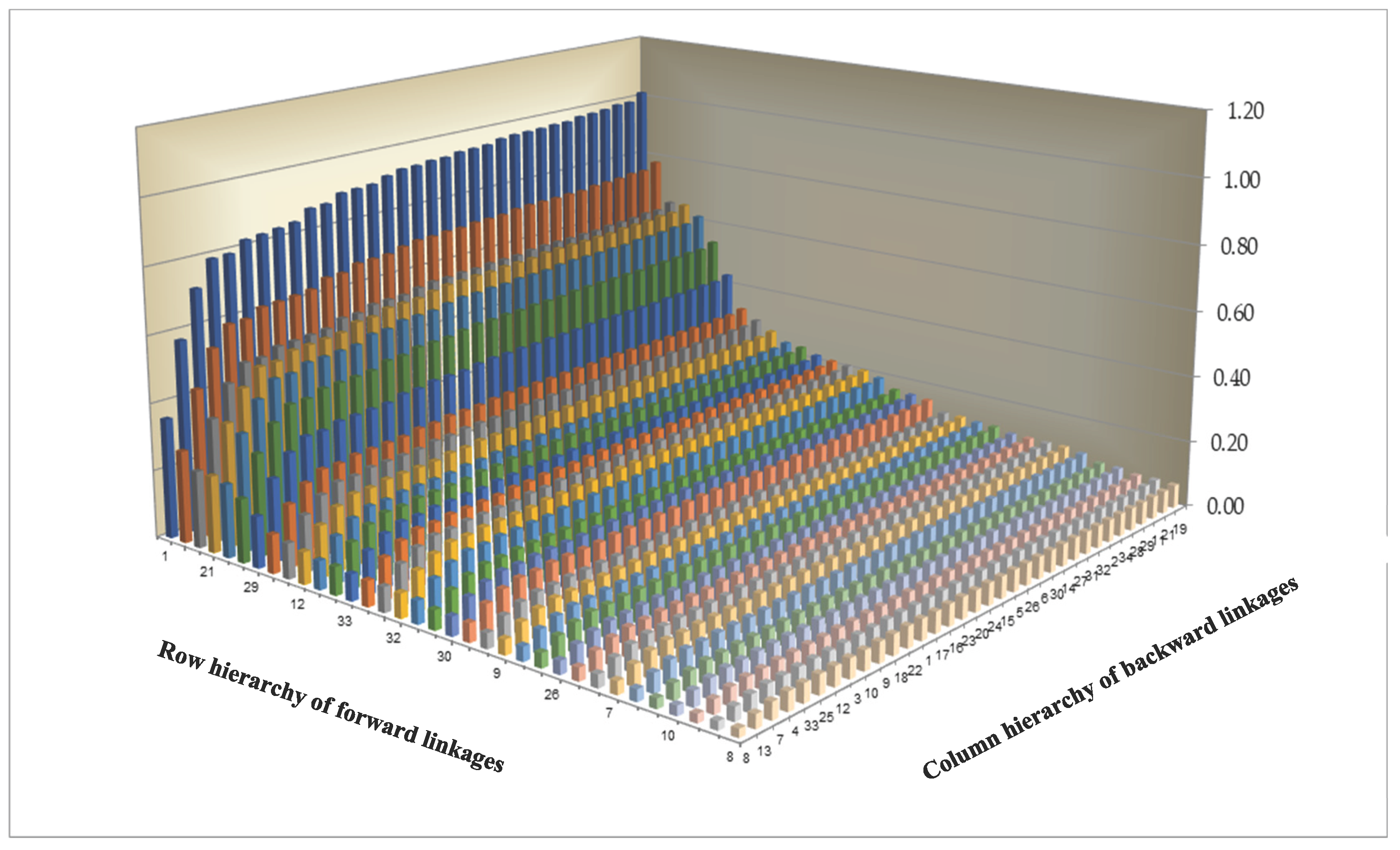
Table 1.
Distribution of target export expansion under different diversification scenarios.
| SECTOR | SAM | Foster | Present | |
| 1 | Agriculture, | 368.63 | 395.47 | 368.63 |
| 2 | Mining and quarrying | 7.19 | 7.71 | 7.19 |
| 3 | Food beverages | 1047.30 | 1089.50 | 1097.42 |
| 4 | Textiles and textile products | 39942.28 | 41551.95 | 41627.00 |
| 5 | Leather, and footwear | 2055.35 | 2138.18 | 2246.94 |
| 6 | Wood and products of wood | 31.40 | 33.68 | 31.40 |
| 7 | Pulp, paper, paper products | 60.09 | 64.47 | 60.09 |
| 8 | Coke and nuclear fuel | 0.15 | 0.16 | 0.15 |
| 9 | Chemicals | 357.24 | 383.25 | 357.24 |
| 10 | Rubber and plastics | 72.66 | 77.95 | 72.66 |
| 11 | Other nonmetallic minerals | 86.28 | 92.57 | 86.28 |
| 12 | Basic metals | 86.52 | 92.82 | 86.52 |
| 13 | Machinery, nec | 60.82 | 65.25 | 60.82 |
| 14 | Electrical and optical equipment | 164.97 | 176.98 | 164.97 |
| 15 | Transport equipment | 209.62 | 224.88 | 209.62 |
| 16 | Manufacturing, nec; recycling | 923.09 | 960.29 | 971.97 |
| 17 | Electricity, gas, and water | 0.00 | 0.00 | 0.00 |
| 18 | Construction | 459.28 | 492.72 | 459.28 |
| 19 | Sale and repair of motor | 0.00 | 0.00 | 0.00 |
| 20 | Wholesale trade | 0.00 | 0.00 | 0.00 |
| 21 | Retail trade | 0.00 | 0.00 | 0.00 |
| 22 | Hotels and restaurants | 388.26 | 416.52 | 388.26 |
| 23 | Inland transport | 0.00 | 0.00 | 0.00 |
| 24 | Water transport | 50.52 | 54.20 | 50.52 |
| 25 | Air transport | 225.61 | 242.04 | 225.61 |
| 26 | Other supporting activities | 0.00 | 0.00 | 0.00 |
| 27 | Post and telecommunications | 3630.26 | 3776.56 | 3783.20 |
| 28 | Financial intermediation | 301.54 | 323.49 | 301.54 |
| 29 | Real estate activities | 0.00 | 0.00 | 0.00 |
| 30 | Renting of M&Eq | 1959.03 | 2037.98 | 2041.56 |
| 31 | Public administration | 561.59 | 584.23 | 588.25 |
| 32 | Education | 1.25 | 1.34 | 1.25 |
| 33 | Health and social work | 0.00 | 0.00 | 0.00 |
| 34 | Other services | 56.05 | 60.13 | 56.05 |
| Total | 53107.00 | 55344.33 | 55344.33 |
Note:Foster denotes the extensive-led diversification scenario, where a total 11% export-demand shock is decomposed into a 7% increase for extensive sectors and a 4% increase for intensive sectors. The other represents the business-as-usual scenario, where the entire 11% shock is distributed proportionally across intensive sectors based on their 2022 export shares. Extensive sectors are those with export shares below 1%, while intensive sectors exceed this threshold in the 2022 SAM. In each scenario, adjusted export values were introduced as shock to the final demand vector in the SAM framework.
Table 2.
Top 6 backward and forward linkage scoring sectors.
| CODE | SECTOR NAME | TOP ORDER BACKWARD LINKAGES IN % |
|---|---|---|
| 19 | Sale of motor vehicles and motorcycles; retail sale of fuel | 114.58 |
| 21 | Retail trade, except for motor vehicles; | 111.79 |
| 11 | Other nonmetallic minerals | 111.76 |
| 29 | Real estate activities | 110.92 |
| 28 | Financial intermediation | 110.48 |
| 34 | Other community, social, and personal services | 110.27 |
| TOP ORDER FORWARD LINKAGES IN % | ||
| 1 | Agriculture, hunting, forestry, and fishing | 187.63 |
| 34 | Other community, social, and personal services | 144.14 |
| 4 | Textiles and textile products | 119.83 |
| 21 | Retail trade, except for motor vehicles; | 119.74 |
| 23 | Inland transport | 114.08 |
| 3 | Food, beverages, and tobacco | 99.27 |
Note: Sectors exceeding the normalized threshold of 100 exhibit above average intersectoral integration. The listed sectors therefore represent the most influential channels in generating upstream input demand and downstream output supply within the economy. See appendix A1 for full table. Source: Author calculation.
Table 3.
Simulation results of top 7 sectors in million US dollars.
| Sectors | FOSTER DIVERSIFICATION | PRESENT DIVERSIFICATION | ||
|---|---|---|---|---|
| Shifts in GDP | Shifts in Labor Income | Shifts in GDP | Shifts in Labor Income |
|
| Agriculture* | 578.93 | 25851 | 567.80 | 25354 |
| Other service* | 454.46 | 2690 | 444.14 | 2629 |
| Retail trade* | 373.83 | 857 | 368.26 | 845 |
| Inland Transport* | 293.83 | 2267 | 291.95 | 2253 |
| Textiles | 722.36 | 20789 | 752.91 | 21669 |
| P&T | 117.33 | 42 | 120.67 | 43 |
| Renting of M&Eq | 108.86 | 64 | 107.77 | 63 |
| Shifts on GDP | 4161.69 | 54590 | 4110.74 | 54442 |
| Total % change | 1.18 | 1.16 | ||
Note: Values marked with an asterisk (*) denote extensive sectors, defined as sectors whose export shares are below 1% in the 2022 SAM. All other sectors are classified as intensive sectors. Importantly, above four sectors also identified as key sectors in the previous section. This means they have the capacity to generate significant ripple effects across the economy, boosting GDP even though their wage transmission remains limited.
Disclaimer/Publisher’s Note: The statements, opinions and data contained in all publications are solely those of the individual author(s) and contributor(s) and not of MDPI and/or the editor(s). MDPI and/or the editor(s) disclaim responsibility for any injury to people or property resulting from any ideas, methods, instructions or products referred to in the content. |
© 2026 by the authors. Licensee MDPI, Basel, Switzerland. This article is an open access article distributed under the terms and conditions of the Creative Commons Attribution (CC BY) license (http://creativecommons.org/licenses/by/4.0/).
Copyright: This open access article is published under a Creative Commons CC BY 4.0 license, which permit the free download, distribution, and reuse, provided that the author and preprint are cited in any reuse.


