
Submitted:
24 February 2026
Posted:
25 February 2026
You are already at the latest version
Abstract
Industrial pouring processes operate under highly dynamic conditions where small deviations can lead to defects, scrap, and production losses. Although modern foundries are equipped with multiple sensors and visual inspection systems, most monitoring approaches remain fragmented, unimodal, and difficult to interpret. Furthermore, annotated anomalous samples in industrial settings are scarce, hindering the development of traditional methods. As a result, many critical pouring anomalies are detected too late or lack sufficient contextual information for effective decision making.
In this work, we propose a multimodal framework for industrial scene characterization that unifies visual information and process signals through a Mixture of Experts (MoE) strategy. First, we deploy an ensemble of specialized modules that collaborate to identify regions of interest, assess pouring quality, and contextualize events within the production process, generating an interpretable description of pouring events. Second, we introduce a novel anomaly detection method for video multimodal data, combining a self-supervised transformer with an outlier-aware clustering algorithm. Our approach effectively identifies rare anomalies without requiring extensive manual labeling.
The resulting information is structured into a digital-twin-ready representation, enabling seamless synchronization between the physical system and its virtual counterpart. This solution provides a scalable, deployable pathway to transform heterogeneous industrial data into actionable knowledge, supporting advanced monitoring, anomaly detection, and quality control in real foundry environments.
Keywords:
multimodal monitoring
; industrial foundry
; digital twin
; mixture of experts
; computer vision
; deep learning
; casting process monitoring
; anomaly detection
; video–sensor fusion
; clustering
1. Introduction
Iron foundry is one of the most mature and widely adopted manufacturing technologies, enabling the large scale production of metallic components with complex geometries and demanding mechanical requirements. Global cast iron production accounts for hundreds of millions of tonnes per year, supplying key industrial sectors such as automotive, energy, railway transportation, and heavy machinery [1]. Within this domain, ductile (also known as nodular) iron has become a preferred material for critical components due to its improved strength, ductility, fatigue resistance, and damage tolerance when compared to grey cast iron [2].
From a process perspective point of view, iron casting manufacturing procedure involves a sequence of tightly coupled stages, including (i) metal melting, (ii) pouring into moulds, (iii) solidification under controlled thermal conditions, (iv) extraction of the solidified part, and (v) subsequent forming or finishing operations. Among these stages, the pouring phase plays a decisive role in determining the final quality of the casting. During pouring, molten metal is transferred into the mould cavity, where its flow behaviour, temperature evolution, and interaction with the mould directly affect filling completeness, microstructural development, and defect formation. Continuous and semi-continuous pouring processes offer significant advantages, such as high production efficiency, improved dimensional repeatability, and reduced energy consumption due to controlled solidification and elimination of auxiliary cooling steps [3,4]. Nevertheless, these benefits come at the cost of increased process sensitivity. Hence, minor disturbances during pouring can propagate downstream, resulting on defects that are difficult to detect and costly to correct.
Despite the extensive industrial experience achieved by foundries, the pouring phase remains particularly prone to quality deviations. Common defects include incomplete filling, cold shuts, poor filling quality, and surface or internal imperfections such as inclusions, porosity, segregation, and thermal cracking [5]. Many of these defects are directly linked to diverse phenomena occurring during pouring, such as stream instability, turbulence, interruptions, or overflow episodes. Importantly, these events often develop over very short time windows and may not be captured by conventional monitoring systems. Notwithstanding, finding these defective cases on industrial scenarios poses a great challenge. This is mainly due to the scarcity of such examples on normal production conditions, which hinders data collection and annotation, requiring hundreds of expert hours. While anomaly detection algorithms are often used, the techniques carried out for detection generally involve low dimensional statistical outlier detection, or depend on, at least, a partially annotated dataset. Furthermore, relying solely on a single data modality (such as sensor signals or visual information) is often insufficient for comprehensive analysis [6]. Many casting-related events and anomalies are better characterized by the fusion of multiple data sources. For instance, sensor readings may indicate changes in casting level or flow rates, while visual data may reveal surface defects or slag layer behavior that are not captured by numerical sensors alone. Therefore, the integration of both sensor and image data, what is known as a multimodal approach, is essential to capture the full complexity of the process and enhance detection performance [7,8].
In this sense, an effective control of pouring parameters (e.g., metal temperature, pouring duration, inter-pouring time, mould alignment, and flow stability) is critical to achieve consistent production quality. In industrial foundries, this control task presents a serious challenge due to the large number of sensors deployed along the production line, the high acquisition frequency of process signals, and the resulting data volume, which complicates real-time interpretation and decision making [9]. Traditional manual inspection or rule-based supervision strategies struggle to cope with this complexity and often fail to provide early warnings of emerging defects [10].
To address these limitations, automated monitoring and intelligent analysis systems have gained increasing attention. Specifically, artificial intelligence (AI) methods, particularly those based on machine learning (ML) and deep learning (DL), offer powerful tools for processing high-dimensional and heterogeneous data streams, enabling improved event detection, anomaly identification, and predictive capabilities [11]. In the context of casting processes, recent works have explored computer vision (CV) techniques for detecting surface defects and pouring anomalies [12,13], as well as sensor-based approaches for real-time supervision of thermal and flow-related variables [14,15].
Nevertheless, many existing solutions remain limited by their unimodal nature. These solutions, which rely exclusively on either sensor data or visual information, often provide an incomplete view of the process [6]. On the one hand, while sensors can capture global trends such as temperature or flow rate variations, they may overlook localised visual phenomena at the mould cup or pouring stream. On the other hand, vision based systems may struggle under occlusions, glare, or variable lighting conditions without complementary process context. For this reason, multimodal approaches that combine image and sensor data have been increasingly advocated as a means to capture the full complexity of industrial processes and enhance robustness [7,8].
Beyond foundry characterization, industrial digitization efforts increasingly emphasise the need for higher-level integration and interpretability. In this sense, digital twins, the virtual representations of physical systems that remain synchronised with their real counterparts, have emerged as a key enabler for monitoring, optimisation, and decision support in manufacturing. Specifically, in casting processes, digital twin principles have been applied to optimise cooling strategies, control solidification behaviour, and reduce defect rates [16,17]. Notwithstanding, effective digital twin deployment requires structured, time aligned, and semantically meaningful data describing not only sensor readings but also events, conditions, and operational context. This highlights the importance of frameworks capable of transforming raw observations into machine readable representations suitable for integration with this type of systems.
Against this background, this work proposes a multimodal framework for the detection and assessment of pouring related anomalies in industrial iron foundry processes. Rather than focusing solely on visual defect detection or isolated sensor thresholds, the proposed approach aims to unify heterogeneous evidences into a coherent and interpretable description of each pouring cycle. The system is designed to operate under real foundry conditions, accounting for occlusions, non-regular operational contexts, and transient disturbances that frequently occur in production environments.
The proposed framework combines visual analysis of pouring scenes with domain specific process signals under a MoE architecture. In particular, a visual detection backbone based on YOLO identifies relevant Areas of Interest (AoI), such as pouring streams, mould cups, and protective elements, while temporal validation through object tracking ensures spatial consistency across frames. Regarding detection of anomalous pouring events, we further encode visual dynamics through self-supervised VideoMAE features [18], enabling compact representation of pouring behaviour over time, which can be used for anomalous event detection through outlier-aware DBSCAN clustering algorithm [19]. Crucially, the limited inductive biases present on transformer architectures allows for seamless integration of multimodal data. Hence, selected sensor signals are integrated to contextualise visual observations and reinforce interpretation through expert informed reasoning. The current approach achieves crucial advancements on several common issues related to anomaly detection on industrial settings. On the one hand, it allows to pin-point potential anomalies, greatly easing the burden on expert annotators to find and tag such events. On the other hand, it presents a valid approach to categorize various normal and anomalous industrial events, successfully integrating and leveraging multimodal information.
The outputs of the different expert modules are aggregated into a structured, digital twin ready JavaScript Object Notation (JSON) representation that captures the state, quality indicators, and contextual conditions of each pouring event. While a full digital twin implementation is beyond the scope of this work, the proposed representation is explicitly designed to support seamless communication with those higher-level systems, enabling future developments in traceability, root-cause analysis, and predictive maintenance.
In summary, the main operational objectives of this work are:
- 1.
- To reliably identify and segment individual pouring events under real industrial conditions.
- 2.
- To detect and track key visual elements required for interpreting pouring dynamics and safety conditions.
- 3.
- To extract interpretable indicators describing stream stability, filling quality, and process compliance.
- 4.
- To find anomalous pouring events through unsupervised multimodal feature learning and clustering.
- 5.
- To unify heterogeneous evidences through an explainable Mixture-of-Experts (MoE) decision framework.
- 6.
- To generate structured outputs suitable for integration with digital twin and supervisory platforms.
The remainder of this paper is organised as follows. Section 2 describes the industrial setup, data acquisition strategy, and methodological components of the proposed framework. Then, Section 3 presents the experimental evaluation of event detection, AoI analysis, unsupervised anomaly detection, and MoE-based decision unification. Finally, Section 4 discusses industrial deployment aspects and limitations, summarises the main contributions, and outlines future research directions.
2. Materials and Methods
To tackle large number of challenges faced by researchers (see Section 1), we adopt a well-known methodology "divide-and-conquer". The main objective, close to the MoE approach, is to simplify the resolution of the original problem by decomposing it into smaller and more manageable subproblems. This strategy allows for a reduction of computational complexity and promotes a structured and efficient problem solving approach. Historically, this methodology has been widely applied to manage diverse challenges, for instance, in legal reasoning [20], mathematical computations [21], and computational problems related to parallel processing [22]. Formally, the general problem is defined as P, which can be expressed as a set of subproblems . Once each subproblem is individually handled and its specific solution is obtained, denoted as , the partial results are systematically combined to construct the complete solution to the original problem:
where C represents the function that combines partial solutions into the final result.
In this work, we decompose the industrial monitoring problem into specialized modules within a multimodal MoE. Each expert represents an independent subproblem, and, their results are unified into a global solution that drives a real-time digital twin of the industrial process. All stages, challenges, and integration phases defined in this work are summarized next and visually represented in Figure 1.
- 1.
- Problem and Challenge Identification. The aim of this initial step is to establish the background and context of the industrial problem to be solved. Analyzing both the multimodal nature of the data (i.e., images, video and sensor streams), as well as other aspects inherent to the problem at hand, such as pouring streams, leaks, overpouring situations or irregular filling patters. In a nutshell, understanding what, how and why must be monitored, providing a clear foundation for each expert specialization.
- 2.
- Knowledge Acquisition. This second phase focuses on obtaining a domain specific and technological knowledge to guide the further research and development of each expert subsystem. Here, high level knowledge is firstly acquired to strongly define the overall workflow of the research. This stages also involves defining data sources, formats and the synchronization requirements necessary for a multimodal integration.
- 3.
-
Challenge Division. Following the divide-and-conquer paradigm, the global problem P is divided into smaller subproblems , each corresponding to a functional expert module that will be included in the MoE framework. More accurately, the definition of each expert will include the following sub-phases: (i) acquisition of specific knowledge, (ii) definition of techniques and experiments, and (iii) results evaluation and analysis.
- Local Image Interpretation and Event Detection. The challenge behind this subproblem focuses on identifying the most probable sources of anomalies. This challenge requires the acquisition of specific knowledge related to visual feature extraction, keypoint detection, and motion-based event discovery. The achieved solution will contribute to enhance the reliability of visual monitoring in complex production settings through the detection of critical areas where irregularities could appear and finally cause a faulty casting.
- Global Environment Evaluation. The second challenge tries to characterize the broader industrial environment and provide and overall process overview. This involves an analysis of plant topology, global process dependencies and large scale events such as line breaks, maintenance operations or overpouring occurrences, among others. This task is an evaluation in a macroscopic level of events occurring during the manufacturing process, assuring that the contextual events are identified and interpreted.
- Manufacturing Evaluator. This challenge tackles quantitative process evaluation and compliance verification. It is is grounded on the acquisition of knowledge related to industrial process parameters, tolerance limits, and production quality regulations. That information should be dependent on the current manufactured reference and must be updated and extracted in real time to be able to characterize the full process accurately.
- Casting Pouring Stream Interpretation. This last challenge involves understanding the dynamic behaviour of molten metal flow during casting operations for unsupervised identification of anomalous events. This work requires the acquisition of expert knowledge, time synchronized video-sensor fusion, self supervised flow dynamics characterization, and categorization of defect topology associated with pouring streams.
- 4.
- Functional Integration through the MoE Unification Metamodel. Once all partial solutions have been computed by each expert, they will be aggregated through the MoE Unification Metamodel. In fact, this metamodel acts as the combination function C (shown in Equation (1)), which merges all outputs into a unified and interpretable representation of the industrial environment.
- 5.
- Digital Twin Synchronization and Continuous Reasoning. The unified output of S as a structured JSON stream, together with the processed visual data, are transmitted to a digital twin, ensuring real-time synchronization between the physical plant and its virtual representation. This phase guarantees that the digital twin accurately reflects the state of the production line at any given moment. Thanks to this data distribution, the twin supports other tasks like predictive maintenance, root-cause analysis, and operational optimization.
- 6.
- Evaluation of Global Results and Dissemination. After a full system integration, a final evaluation phase is carried out to encourage the global performance of the Multimodal Industrial Monitoring System with MoE. This final phase includes (i) a quantitative evaluation, (ii) qualitative evaluation, and (iii) results dissemination.
2.1. Data Acquisition and Capture Environment
The data used in this work was acquired on a commercial sand-casting production line. To preserve industrial confidentiality, site specific identifiers (for instance, plant name, exact location and proprietary process parameters) have been omitted and, in contrast, they were replaced by aggregated descriptors and representative statistics. Despite this fact, authors provide enough methodological details to enable the replication of the proposed approach.
Casting is one of the oldest and most fundamental manufacturing processes, in which molten metal is poured into a mold cavity that reproduces the desired shape of the final component [23]. Among different casting techniques, green sand casting remains as one of the most widely used due to its cost effectiveness, reusability of materials, and suitability for mass production [24,25]. In this process, the mold is made of a mixture of sand, clay, and water (also known as green sand). This mixture provides enough strength and plasticity to retain the shape during metal pouring and cooling. A modern variant of this method is the vertical molding process, where the sand molds are created and aligned vertically in a continuous production line. This configuration, usually associated with DISA moulding machines, enables a high speed production (close to an average of 550 moulds per hour) with excellent dimensional accuracy and automation capabilities [26]. The vertical arrangement allows molds to cool down as they move continuously over a conveyor. Figure 2 illustrates the schematic of the vertical sand-casting line used for this study.
There are several types of metals used to create castings. The material used in our case is nodular cast iron, also known as ductile iron. This metal is a ferrous alloy characterized by the spheroidal morphology of its graphite inclusions. This microstructural feature provides a superior combination of strength, toughness, and ductility compared to gray cast iron, making it ideal for automotive, hydraulic, and structural applications [27,28].
The molding line operation starts with the moulding machine. It compacts green sand around a pattern, and eject the created mould to the conveyor. The formed moulds advance along the mould train until they reach the pouring station, where a press-pour mechanism deposits the molten metal into the pouring cup. Then, gravity pulls down the metal which ends up filling the cavity inside the mould. During pouring, a protective cover know as tile, is placed over the next pouring cup to prevent unintended spillage of metal into downstream moulds. This reduces the risk of cross contamination between them. The quality of the pouring operation is critical as bad pouring procedures frequently cause defects. These may have different consequences for component performance [5,23,25,29], and can be categorized as follows:
- Severe (structural) defects: phenomena that may cause catastrophic failure or render a part as unusable. For instance, this group includes carbide formation or hard brittle phases, compromising toughness and increasing the risk of premature fractures under load; cold shots, causing weak discontinuities due to incomplete coalescence of metal streams; shrinkage porosity, voids produced by volume contraction during the solidification stage, which cause leakage; and gross lack of material due to underfilling.
- Functional defects: defects that affect the final functionality of a part or the subsequent finalization operations, such as machining. Some examples are (i) hard inclusions (for instance, slag, sand inclusions or oxides) and (ii) local carbide pockets that damage cutting tools or reduce the service life of a part. All those defects are usually formed by a turbulent pouring, inadequate filtration, or a poor gating/riser design.
- Aesthetic defects: surface flaws or minor inclusions, such as light sand inclusions or small blow-holes, among others. These do not compromise mechanical performance but may require rework to solve them or cause the rejection of a component.
An automated monitoring system that combines video evidences of the pouring process with synchronized sensor signals provides a practical route for early detection of these faults, supporting root-cause analysis and corrective actions on the line [13,15]. In order to handle this kind of monitoring, the video camera is positioned to capture the pouring event, the filling level of each mould, and any special events like visible overflow or spillage. Simultaneously, process sensors (e.g., temperature, flow/weight, among others) and the material flow behaviour are synchronized with the video to try to identify any problem along the pouring area. Figure 3 illustrates how this pouring monitoring system is deployed in a real-life green sand foundry plant. The resulting multimodal dataset is used throughout this paper, and is the basis for model training, anomaly detection and the real-time updates sent to the digital twin.
The data used was captured at the selected foundry by a centralized industrial DataLogger-based acquisition system that was configured to communicate with the plant Programmable Logic Controllers (PLCs), map their memory zones and register the relevant signal tags (i.e., digital I/O, analog channels, counters and event markers). Moreover, network cameras were integrated into the same acquisition topology via Real Time Stream Protocol (RSTP) interfaces, and both camera streams and sensor traces were timestamped and recorded into a centralized storage with metadata descriptors. Unfortunately, recorded data does not index pouring events nor mould identification, hence, video frame ranges, synchronized sensor windows and derived descriptors (e.g., filling time, peak flow, temperature profile) cannot be directly matched with a real casting event evidence registered in the Manufacturing Execution System (MES) database.
Figure 4.
Screenshot of the centralized DataLogger capture software used in this study. The panel shows a synchronized video frame of the pouring area alongside three representative process signals that correspond to typical pouring telemetry (e.g., melt temperature, stopper mechanism, and hydraulic/pressure channel). All streams are time-aligned and indexed to the active mould identifier. Note that all signal labels are intentionally obfuscated for confidentiality.
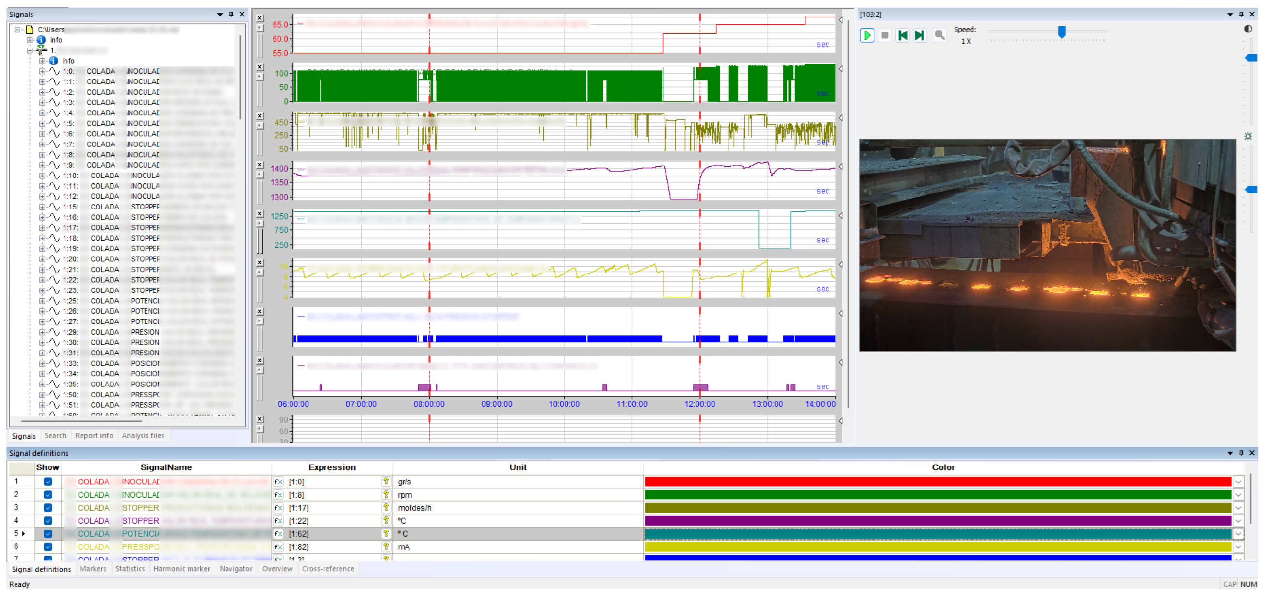
Next, we provide a detailed explanation of the contents of the dataset used in this study, including data types, acquisition settings, and synchronization strategy to ensure full methodological reproducibility. Nevertheless, to preserve industrial confidentiality, exact counts and specific parameters are omitted and replaced by aggregated descriptors and representative statistics.
Video Recordings
The video dataset comprises approximately 12 hours recorded across 2 sessions under normal operating conditions (with 8 and 4 hours respectively). All sequences were acquired at a resolution of pixels and 20 fps, encoded with the H.264/AVC standard at bitrates ranging between 3.0 and 3.2 Mbps. No audio tracks were included in the recordings. Both videos show a stable keyframe period of 1.5 s, ensuring temporal alignment with sensor data. In both recordings, the camera placement corresponds to the field of view illustrated in Figure 3, capturing the pouring stream, the tile/cup area, and the first produced moulds in the beginning area of the conveyor (all detailed in Figure 2).
The captured footage represents the continuous operation of the vertical green-sand moulding line producing nodular iron castings of different references and cup geometries. Recordings display typical working conditions of the industrial casting line, including changes in lighting due to natural illumination and the radiant emission of the molten metal, turbulent jets in a pouring stream, sporadic metal splashing, overflows, and short production stops during reference changes or mould rejection. The lighting control of the camera is automatic and maintains overall visual consistency despite diurnal variations. Besides pouring events occurring approximately every 5 seconds, these videos also recorded short pauses such as maintenance interventions or reference changes, among others. This special events are ∼2% of the total time. In addition, the dataset also includes both regular and irregular pouring sequences, covering normal variability of the foundry day-by-day work. Although no event tags are included with the data, we were able to identify the special using CV and the synchronized records from the process sensors. Furthermore, reference changes are visually recognizable due to a series of empty moulds and a manual mark on the conveyor. With this, we have identified 14 such events, confirming the visual stability of the setup and the absence of camera shake or abrupt illumination changes. All videos are stored in raw format without stabilization or image corrections to preserve authentic process dynamics and facilitate a further reproducible multimodal analysis.
Crucially, the precise synchronization of video and sensor data enables robust multimodal analysis. By correlating visual features, like pouring stream shape, with process variables, such as flow rate, this alignment provides the foundation for effective digital twins and data-driven anomaly detection, supporting predictive quality control in real production environments.
Sensor Recordings
Parallel to video acquisition, a complete set of process and control signals was recorded from the plant. These signals were sampled at an approximate rate of 2.5 Hz and they are synchronized with the video frames using shared timestamps. The gathered dataset contains 155 distinct process variables, reflecting both continuous and discrete values across the foundry line. Although the precise sensor identifiers are hidden for confidentiality reasons, the signals can be grouped into several functional subsystems that are representative of a vertical green-sand casting process. Table 1 describes the approximate distribution of signals among these subsystems and provides representative examples of each group. These can be summarized into four groups:
- Moulding area, which includes critical variables for maintaining a consistent mould density and ensuring dimensional integrity before pouring.
- Pouring process, including variables related to the press-pour unit and supervising molten metal conditions. These parameters directly determine casting quality and correlate strongly with the aforementioned casting defects.
- Conveyor and cooling line, which monitor mould evolution after pouring.
- Auxiliary and safety systems signals, which provide contextual information about line stops and maintenance events.
- Quality and traceability signals identifies reference changes, rejected moulds, or operator interventions, facilitating synchronization between the physical process and the third-party systems.
2.2. Global Context Evaluation
Then, we focus on understanding the global production context in which these operations occur. This stage handles the classification of the overall operational state of the foundry line from visual information. Its specific goal is to distinguish whether the process is running under normal conditions or affected by contextual disturbances such as maintenance tasks (which might create operator occlusions), over-pouring, or technical stops. This enables both real-time alerts and the exclusion of anomalous sequences from subsequent analytical modules. In fact, this classification enables filtering non-productive intervals and contextual anomalies that could otherwise distort quality assessment or multimodal fusion with process signals. We have defined 4 contextual states, which represent the production workflow itself (see Figure 5):
- 1.
- Normal operation, corresponding to regular casting cycles where pouring, mould transport and cooling proceed without interference.
- 2.
- Maintenance, when operators enter the scene or perform manual adjustments, often producing occlusions that compromise visual analysis.
- 3.
- Overflow, describing situations where molten metal splashes outside the mould cup, typically caused by misalignment or excessive pouring rate.
- 4.
- Stop line, representing planned or unplanned halts such as pattern changes and safety stops, among others. Usually, moulds are manually marked as rejected with chalk.
To automate this contextual classification, several image classification architectures were considered. Traditional convolutional networks such as ResNet-50 [30] and EfficientNet [31] have been the foundation of manufacturing vision systems due to their accuracy and fine tuning capabilities. Nevertheless, more recent transformer based architectures such as ViT [32] and ConvNeXt [33] introduce improved global attention mechanisms, achieving outstanding accuracy in large scale datasets but with significant computational demands. Hence, they are less suitable for real-time inspection problems. On the contrary, the YOLOv11-class [34] model offers an optimal balance between precision and latency, optimized for real-time industrial deployment. It also ensures architectural compatibility with the area detector and classifier used in this work (see Sections 2.3.2 and 2.4.1), simplifying deployment and reducing hardware requirements.
The dataset employed for training comprised approximately 262,600 images extracted from the 4-hour video recording. Each frame was manually labelled by a foundry expert into one of four categories: normal operation (212,000 samples), overflow (45,000), maintenance (2,500), and stop line (2,100). The data were split into training, validation, and test sets with a 60/20/20 ratio. We fine tuned the pretrained YOLOv11 backbone, employing the standard Ultralytics augmentation strategies (for instance, including random scaling and cropping, horizontal flipping, HSV adjustments, gaussian blur and mosaic), which have shown to significantly improve robustness under varying illumination (e.g., molten metal glare) and occlusions commonly found in casting environments [34].
In summary, this module completes the visual perception pipeline by attaching a contextual state to every detected pouring event. As a result, only segments corresponding to normal operation are forwarded to quality evaluation and MoE fusion, while frames affected by maintenance tasks, line stoppages, overflows, or camera occlusions are automatically flagged and excluded.
2.3. Local Image Interpretation and Event Detection
This section addresses the local analysis of the video stream, where visual information is structured into meaningful process entities. It comprises 2 complementary stages: first, the Pouring Event Identification, which temporally segments the continuous sequence into discrete casting cycles; and second, the Detection of AoIs, which spatially isolates the relevant regions within each event for subsequent interpretation. Together, these stages transform raw video data into semantically organized information that serves as the axes for a high level modelling and process understanding.
2.3.1. Pouring Event Identification
The final objective of this stage is to enable the automatic interpretation of manufacturing visual content through event delimitation within the pouring process. This stage aims to temporally segment the continuous video sequence into well-defined pouring cycles that correspond to real process operations. We denote these segments as pouring events. From this stage, every frame is processed not as an isolated observation but as part of a dynamic process where recurrent operations occur under industrial constraints, since each production cycle can be represented as a repetitive task of mould generation, pouring, transport, and cooling. Formally, we define the set of pouring events as , where each event represents a complete pouring operation within the production line. Each event is delimited in time by the lowering and subsequent rise of the pouring unit, specifically, , with the instant when the pouring unit begins its descent and when the filled mould leaves the pouring zone or the next empty mould arrives. During this interval, we observe a multimodal sequence of variables:
where denotes the video stream, the stream shape descriptors, the environment characterization indicators, the process variables such as pressure, temperature, among others, and the quality measurements related to the current production reference.
In theory, the acquired signals can provide direct temporal markers. Nevertheless, in practice, industrial data acquisition often suffers from synchronization drift, missing packets, or timing mismatches between video and process signals [39]. Therefore, a double check provided by a artificial vision-based approach was adopted to autonomously identify event boundaries by analysing image motion and frame similarity.
For this purpose, several algorithms were considered to determine an optimal trade-off between accuracy, robustness, and computational efficiency. One common approach is dense Optical Flow (OF), such as Recurrent All-Pairs Field Transforms (RAFT) [40], which computes pixel-wise motion vectors across consecutive frames. OF has become a benchmark for high precision motion estimation in industrial and robotic inspection tasks, as it offers a fine grained motion tracking. However, this approach exhibits high computational cost and large memory footprint, limiting real time deployments on full HD sequences. Although this fact is discussed in [41] and authors provide new optimization possibilities, we decided to discard it.
Alternatively, simple frame or histogram difference methods were also tested as baseline strategies for motion quantification, given their minimal computational load. Notwithstanding, as noted by Karbalaie et al. [42], such techniques are highly sensitive to the molten metal, due to the produced glow and automatic exposure corrections by cameras, which may trigger false positives.
Finally, we consider the Structural Similarity Index Measure (SSIM), which has been validated as a perceptual metric for detecting state transitions in industrial video monitoring [43,44]. SSIM quantifies luminance, contrast, and structural coherence between successive frames, enabling detection molds and metal movements. Recent studies have validated its robustness against illumination fluctuations and flicker noise in real production environments [45]. Its low computational complexity makes it particularly well suited for embedded industrial monitoring systems.
To further optimize performance, the analysis was restricted to a dynamically defined Region of Interest (ROI) enclosing the pouring stream and adjacent mould cup, as illustrated in Figure 6. In addition, the pouring stream region is detected dynamically through an adaptive ROI strategy. This allows the system to automatically adjust to camera viewpoint changes, ensuring that the pouring zone and the first poured mould exiting the scene remain consistently localised even under shifts in perspective or framing. Hence, the performace is improved when reducing redundant pixel processing and only maintaining focus on semantically relevant areas [39,45]. In our implementation, the ROI position is automatically updated based on the previously detected stream centroid, creating our own self adaptive mechanism that maintains consistent spatial tracking.
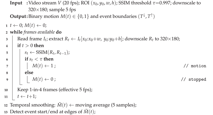
Algorithm 1 summarizes the final adopted implementation using SSIM motion detector. The algorithm processes consecutive frames within a small ROI enclosing the pouring zone and computes their structural similarity to quantify inter frame changes. Motion is declared whenever the similarity drops below a threshold , which effectively distinguishes between static and dynamic phases. Temporal smoothing, carried out as a 5 frame moving average, reduces spurious transitions caused by exposure fluctuations or molten metal glow. Finally, to ensure lightweight processing, we downscale the ROI region down to px. This configuration provides a robust and computationally efficient solution that runs in real time while preserving accurate event delimitation. The resulting binary signal marks the start and end of each pouring cycle and serves as the temporal reference for subsequent analysis and synchronization with sensor data.
| Algorithm 1: SSIM-based motion detection within ROI (casting event delimitation) |
 |
2.3.2. Detection of Areas of Interest
Once the pouring events are detected, the next step is concerned with the interpretation of the visual content within each event. Despite the high spatial richness of each frame, large regions of the image correspond to static background or machine structures with little relevance to measure the quality of the pouring process. Therefore, this analysis must be focused on specific Areas of Interest, which correspond to the relevant regions where molten metal interacts with the mould and auxiliary devices during the pouring stage (see Figure 7), such as:
- Mould cup(s): visible holes that are positioned in front of the camera on arrival to the pouring area. They may appear empty, partially, or fully filled. Monitoring their fill level provides contextual information on pouring accuracy and metal delivery consistency.
- Pouring stream: the continuous jet of molten metal descending from the pouring unit. Its shape, thickness, and turbulence reflect process stability and are strongly correlated with casting defects.
- Tile (splash guard): a protective device that prevents splashes or secondary jets from contaminating the next mould.
- Incoming mould cup: the next cup that becomes visible when the conveyor advances. Occasionally, early contact with residual metal or splashes may occur, and its early detection allows triggering predictive alarms.
To automatically identify these areas, several object detection architectures were considered, spanning both two-stage and one-stage paradigms. Two-stage models, such as Faster R-CNN [46], first generate region proposals and then classify them, achieving excellent accuracy but at high computational cost. In contrast, one-stage models like SSD [47] or the YOLO family [48] predict bounding boxes directly over feature maps, delivering competitive precision at significantly lower latency, making them ideal for industrial applications with real time constraints. In particular, the YOLO family consistently provides the best balance between inference speed and detection accuracy [47,48], outperforming SSD and achieving significantly lower latency than Faster R-CNN. Given the real time operational requirements of our foundry line, YOLOv11 was selected as the detection backbone. For the initial proof-of-concept, we adopted the lightweight YOLOv11-nano variant to evaluate feasibility and runtime, leaving open the possibility of upscaling to larger versions for accuracy improvements.
The model was trained using a dataset of approximately 258,000 frames extracted from a 4-hour production video. Due to manual annotation of such volume is prohibitive, we employed a two-stage semi-supervised strategy similar to the human-in-the-loop approaches described by Lee et al. [51] and Liu et al. [52]. The first phase involved 17,000 manually labelled frames covering diverse conditions (illumination, references, turbulence levels). The second phase used the preliminary detector trained on those to automatically label the remaining frames, which were then manually reviewed and corrected to create the final training corpus. This iterative refinement increased annotation efficiency and ensured accurate bounding boxes. In summary, the combination of the pouring event and area-of-interest detection yields a highly structured video representation aligned with the actual foundry workflow. This pre-processing stage eliminates irrelevant visual noise, focuses computation on semantically meaningful areas, and supplies clean and time-aligned visual features to be fed the subsequent models responsible for pouring quality assessment and the further integration with the MoE framework. An example of detected AoIs can be seen in Figure 8.
2.4. Areas of Interest Visual Classification
Next we aim to perform local classification within each of the detected AoIs to characterize their visual state in the manufacturing process. This step focuses on the static regions extracted from the YOLOv11 detections (see Section 2.3.2), specifically, the mould cups and the next incoming cup. It was excluded the pouring stream, which requires a temporal analysis and is described separately in Section 3.4.
2.4.1. Mould Cup Filling State Classification
Each detected mould cup is analysed to determine its filling level condition. The classes considered are empty, medium, full, and overpoured, illustrated in Figure 9. These states represent, respectively: (i) a mould cup that has not yet received metal, (ii) one that has been partially filled, (iii) a correctly filled cup, and (iv) an excessive pouring resulting in overflow or splashing.
This classification step is essential because the mould path is exposed to multiple sources of variability that may compromise casting quality. For instance, mechanical vibrations of the conveyor, mould misalignment, sand defects, or microleakages along the pouring channel. This issues can cause deviations from the expected filling level. Therefore, tracking the state of every mould cup across the detected pouring event allows early detection of anomalous behaviour thanks to the continuous identification of potential metal losses along the line, and the verification that the pouring stream reaches the mould under the required process conditions.
To this end, we employ the same backbone and hyperparameter configuration described in Section 2.2, again, YOLOv11 classification branch was employed for this task. The data consisted of approximately 184,041 annotated mould cup instances, divided according to the following distribution: 59,414 empty, 50,522 medium, 49,877 full, and 24,228 overpoured. The data were randomly partitioned into training (60%), validation (20%), and testing (20%) subsets. In the same way as in previous classification problems, augmentation strategies such as brightness jittering, small angle rotation, and contrast scaling were applied to improve generalisation under variable illumination and exposure conditions typical of the foundry environment.
Overall, the mould cup classifier extends the AoI level perception layer by offering a fine grained interpretation of each mould’s filling state. Together with the incoming cup detector and the pouring stream analyser, this component contributes to a unified and temporally aligned understanding of the pouring operation, later integrated by the MoE framework.
2.4.2. Incoming Mould Cup Classification
In addition to the active pouring zone, the next incoming mould cup is also analysed to anticipate potential quality issues before pouring begins. Detecting metal residues inside an incoming mould cup is critical because even small droplets of prematurely solidified metal can generate severe casting defects. Residual metal may obstruct proper flow during the next pouring, promote cold shut defects when fresh metal meets already solid fragments, or induce local porosity by disrupting thermal gradients inside the mould. Moreover, splashes accumulated during previous cycles may indicate instabilities in the pouring stream or mould alignment issues. For these reasons, the incoming mould cup must be monitored to ensure that its condition does not compromise the quality of the next cast piece in the production sequence.
Two states are considered, as illustrated in Figure 10: (i) OK, when the mould cup is clean and ready for filling, and (ii) Warning, when metal residues or splashes are visually detected inside it. Early identification of such conditions enables predictive alarms and improves downstream traceability of potentially defective moulds. This classifier allows to reliably distinguish clean cups from those containing metal residues even under strong brightness variations or partial occlusions.
The dataset used for this task included 280,363 cropped AoI samples, where 93% represent OK samples, and 7% are Warning ones. Each class was divided into training, validation, and test subsets with a 60/20/20 ratio. Training was performed by fine tuning ImageNet-pretrained YOLOv11 weights, applying similar augmentation strategies as in Section 2.4.1 to ensure robustness as we applied for the pouring cups.
Altogether, the incoming cup classifier acts as an anticipatory safeguard within the pouring pipeline. By detecting hazardous pre-filling conditions several seconds before the molten metal reaches the mould, it enables the system to flag potential risks earlier than any downstream inspection stage could. This early warning capability not only reduces scrap generation but also provides the MoE with critical contextual evidence that enriches the final event evaluation and strengthens decision reliability across the entire production chain.
2.5. Pouring Stream Interpretation
In this section we focus on characterizing the pouring stream. Beyond common issues like overflow, maintenance, or sudden drops, defective streams in industrial settings can take on many subtle forms, for example forked, unaligned, crooked, turbulent, or interrupted flows. These variations are visually distinct but often hard to categorize using traditional methods. Complicating matters further, industrial environments typically produce very few defective samples, making it difficult to even confirm their presence in the data. This in turn, requires an extensive annotation process going through hundreds or thousands of normal samples until the anomalous ones are found. As a result, we approach this problem from a different perspective, more akin to anomaly or outlier detection, hypothesizing that this perspective may help uncover not only known defects but also unexpected or rare anomalies.
Our approach can be summarized into two steps. First, we employ an autoencoder-like architecture for the characterization of jet stream dynamics. In particular, by solving a simple self-supervised reconstruction task, the network learns to model the inherent behaviour and dynamics of molten metal, producing multimodal representations of the video and sensory information. Then, we drop the decoder and extract features for each sequence at the output of the encoder. These are fed into a clustering algorithm to properly categorize them into different semantically coherent classes, which we can use to analyze the different types of normal and anomalous samples.
2.5.1. Background
Most anomaly detection techniques rely on having a clean set of normal samples [55,56]. For example, reconstruction-based methods [57,58] use autoencoders trained on normal data to flag anomalies via reconstruction error, while one-class classification [59,60] and normalizing flow [61,62] approaches also depend on clear separation between normal and anomalous data to learn discernable distributions. However, when the dataset is noisy or contaminated, these methods often struggle [63,64]. Some recent works address this by explicitly filtering out anomalies (like in [65,66,67]) or mitigating their impact during training (as it was describen in [65,68,69]). However, these methods either disregard information provided by the anomalous samples, or require a priori knowledge of the contamination degree. Furthermore, many of these works have only been tested on MNIST [70], CIFAR10 [71], or COCO [72] where one class is used as normal samples, and other classes are used as anomalies. While some have been evaluated on MVTec [73], the application of these techniques may not directly translate into our industrial video scenario.
Traditional outlier detection [74] often relies on unsupervised techniques like feature extraction followed by clustering, which are especially useful when labeled data is scarce. This technique has also been used for anomaly detection [75,76,77], as both terms are often used interchangeably. In visual data, feature extraction can be done using supervised models pre-trained on large datasets, but these can be biased towards supervised tasks, hence they may miss the fine-grained, low-level details needed for industrial contexts. Unsupervised methods trained on natural generic images also tend to struggle when applied to specialized domains [78]. We believe that a more promising approach is to learn features directly from the target data, most commonly done by leveraging convolutional autoencoders (e.g., [79,80]), though in our case, we explore transformer-based architectures, as they have been shown to better handle non-local interactions in the data [81].
Regarding feature extraction, supervised approaches are often impractical in our setting. Annotating casting videos requires expert knowledge and is prohibitively expensive, while models trained on labeled data tend to learn task-specific features that do not generalize as well [82]. Similarly, relying on pre-trained models, even those trained with self-supervised objectives, faces the same limitation: most existing models are trained on natural images or videos [83], which differ significantly from our industrial setting. This domain gap makes direct transfer ineffective for capturing the fine-grained patterns relevant to molten metal jet streams. Alternative self-supervised strategies, such as contrastive or joint-embedding methods, excel in categorical tasks, specially in object-centric datasets [84] but struggle in other situations [85,86]. In contrast, generative approaches have shown superior performance in tasks requiring detailed spatial understanding, such as object detection or segmentation [87]. Given that our goal involves characterizing fluid dynamics and texture-level variations, we require a method that preserves high-frequency details rather than focusing solely on global semantics [88].
To address these challenges, we adopt VideoMAE (Video Masked Autoencoder) [18], a self-supervised framework designed for video representation learning. VideoMAE reconstructs masked spatio-temporal patches, encouraging the model to capture fine-grained texture and motion cues essential for understanding jet stream behavior. Its transformer-based architecture effectively models long-range temporal dependencies [88] and supports seamless multi-modal integration, which is advantageous for incorporating additional sensory data [89,90]. Furthermore, its self-supervised nature allows us to exploit large volumes of unlabeled casting videos, learning domain-specific representations without costly annotation. These properties make VideoMAE particularly well-suited for our application, where meaningful spatio-temporal features are critical for downstream clustering and anomaly detection.
Once features are extracted, clustering is typically used to separate normal from anomalous samples. K-means is widely used but presents several limitations. It forces all data into clusters, assumes clusters of similar size, and requires the number of clusters to be specified in advance (see also Section 3.4). Alternatives like CBLOF [91] and LDCOF [92] offer more flexibility but are harder to tune due to excessive hyperparameters. Density-based methods such as DBSCAN [19], Density Peak Clustering [93], HDBSCAN [94], and OPTICS [95] are better suited for identifying outliers directly. Among these, DBSCAN stands out for its robustness and simplicity, and although it has been used extensively in prior work (e.g., [96,97,98]), we have not seen it applied to video data. We believe one reason for this gap in the literature may be related to the curse of dimensionality (see [99] for an intuitive definition) affecting common distance metrics used in clustering algorithms [100]. Although this has been challenged in other works [101], and we hypothesize that employing a neural network to embed the visual data may help alleviate this problem [102,103].
To the best of our knowledge, there are very few previous works with similarities to our proposal. Current approaches to clustering-based video anomaly detection are generally limited to dual-stream autoencoders paired with parametric clustering methods, like K-means or Spectral, that require a fixed number of clusters [104,105]. While isolated attempts have been made to incorporate spatiotemporal features via 3D convolutions [106] or distance-based outlier removal [105], these methods lack density-based adaptability and do not fully exploit modern transformer architectures. We propose a novel framework that leverages multi-modal video transformers and utilizes DBSCAN to enable density-based outlier detection.
2.5.2. Data Preparation
The position of the pouring stream varies along the moulding sessions. For this reason, for each pouring event defined in Section 2.3.1, we leveraged the YOLOv11 detector trained in Section 2.3.2 to extract RoIs of the pouring stream from each frame. To ensure temporal consistency and avoid false detections, we employ a simple algorithm to combine the AoI detected on each individual frame from the pouring event. For each new detection, a decision is made to keep it only if: a) the detection confidence is above a threshold (in practice 0.5), and b) the IoU with the accumulated box (the union of all previously detected boxes within the current pouring event) is above a given threshold (in practice 0.6). When the detector fails to detect a pouring stream for more than a margin of 10 frames, we consider the pouring event is over. As a final cleanup step, we compute the average detected box and remove any outlier box (those for which IoU with the average is below a threshold). The final AoI is computed as the union of the remaining boxes.
2.5.3. Methodology
VideoMAE
In our implementation, VideoMAE [18] processes sequences of 16 frames extracted from the YOLO-detected stream regions, producing rich spatiotemporal embeddings that encode both the spatial characteristics of the stream shape and its temporal evolution. The encoder architecture transforms these video clips into high-dimensional feature vectors that capture subtle variations in stream behavior, such as flow stability, turbulence patterns, and directional changes. These embeddings serve as the foundation for our clustering analysis, where similar behaviors are grouped together, enabling the identification of distinct operational modes and the detection of anomalous patterns that deviate from normal casting conditions.
The temporal modeling capability of VideoMAE is particularly valuable for stream analysis, as casting anomalies often manifest as temporal irregularities rather than instantaneous defects. By encoding sequences rather than individual frames, the model can distinguish between normal flow variations and genuine anomalies, such as bifurcations or unstable flow patterns that develop over time. This temporal awareness, combined with the model’s ability to learn from unlabeled data, makes VideoMAE an ideal choice for developing robust, interpretable characterizations of industrial streams that can support both real-time monitoring and predictive maintenance applications.
In a nutshell, VideoMAE masks part of the input video and reconstructs it using an encoder–decoder architecture. The encoder learns a compact representation of the input, while the decoder reconstructs the masked tokens from that representation. The video input is initially partitioned into non-overlapping spatio-temporal patches. Each patch is passed through a lightweight convolutional network (CNN) to produce an embedding, yielding , where denotes the number of resulting patches (hereafter denoted as tokens) and their feature dimension. A portion of these tokens is then randomly masked, and only the unmasked tokens are provided to the transformer encoder . Importantly, the masking scheme suppresses an entire spatial location across all time steps to prevent the model from exploiting information carried over from nearby frames (i.e., shortcut learning [107]). The decoder subsequently consumes both the visible tokens from the encoder and a set of learnable mask tokens to reconstruct the original video. The mean squared error (MSE) loss is used between the masked and reconstructed tokens:
where p is the token index, is the set of masked tokens, I is the input image, and is the reconstructed one. The weights are initialized with the ViT-B pre-trained model on Kinetics-400 [108] (1600 epochs) provided by the authors on the model zoo [109]. We then remove the decoder and keep the final features at the output of the encoder.
Sensory data
We employ the implementation provided by the authors in [109]. To include sensory data, we sample readings from the same time-range as the frames: where is the number of sensors used and is the number of readings sampled during a given video sequence. We use a fully connected network to map the readings into the same dimensionality as the visual tokens, resulting in . These are then simply enhanced with sinusoidal positional encodings [110] and concatenated together with the visual tokens. As the number of sensory tokens is notably smaller than that of visual tokens, we also add a weight to the loss, weighting the contribution of each element to the loss. In this manner, the final loss results in where and are the weights for the visual and sensory loss respectively, set in practice to 1 and 5.
For the sensory data we combine two masking strategies. First, masking tokens as done for the visual ones, resulting in a reduced set of sensory tokens. However, the model could simply learn to interpolate between readings of the same sensor. For this reason, we also mask entire sensors across all temporal tokens. In order to preserve the temporal dimension across tokens, we choose to mask by setting the values of those sensors to 0. We hypothesize that, with this combined approach we force the model to better understand visio-sensory relationships to properly infer the values of the missing sensors and visual information as a whole. We use a masking ratio of 82% for visual tokens and 45% for sensory data. The remaining parameters were left as in the original paper.
Clustering
Once training converges, the decoder is discarded and the encoder processes full, unmasked sequences. Spatially pooled visual tokens and sensory features are extracted, normalized, and further reduced, while temporal features are preserved. The resulting representation is fed into a clustering stage (see Section 3.4). DBSCAN is adopted as the primary method with empirically tuned parameters, and k-means is evaluated as a baseline.
2.6. Mixture of Experts
Once the pouring events have been identified thanks to the movement detection (see Section 2.3.1) and the relevant AoIs detected and classified (Section 2.3.2), the next step focuses on evaluating the manufacturing outcome of each cycle. Specifically, this stage analyses both (i) the visual state of each detected element involved in the pouring operation and (ii) the process performance according to the foundry control plan. The resulting measurements is a structured set of variables that, lately, will be employed by the MoE system and its integrated rule-based expert system for data aggregation, correlation and knowledge generation. The overall interaction between the different experts and the supervisory MoE layer is summarised in Figure 11, which illustrates how heterogeneous assessments are combined into a single event level decision.
Evaluation of AoIs and pouring stream conditions.
For every detected pouring event , the visual elements are interpreted to produce a set of semantic labels. In this case, the pouring stream is characterised by the anomaly score computed in Section 3.4: .
Moreover, the number of interruptions in the stream is also quantified as , while the total pouring duration is defined as:
Furthermore, each mould cup in the conveyor is tracked before, during, and after reaching the pouring zone, giving the identification of its filling state like
The following cup (i.e., the incoming mould cup) is simultaneously monitored to detect undesired metal droplets or premature splashes, producing a binary safety flag , where denotes a warning condition. Similarly, the presence or absence of the tile (also known as the splash guard) is inferred to contextualise if the protection mechanisms are present.
These indicators allow tracking each mould individually along the the visible span of the conveyor belt captured by the camera, detecting undesired metal losses or incomplete filling throughout its trajectory over the visible part of the conveyor. This information is preserved and later aligned with the production references for final traceability.
Evaluation of process performance and control limits.
Beyond the visual part, each pouring event is checked against the process constraints defined in the foundry control plan. For every event , the following temporal variables are computed:
These variables are compared against the acceptable ranges established by the specific control specifications of the produced reference:
When the process exceeds these tolerances, process deviations are identified. Those deviations can be translated into special and also risky situations. Additionally, stream interruptions are also recorded through and their temporal position related to the event. These cuts are often correlated with turbulence, clogged nozzles or thermomechanical instabilities. In addition, a prolonged idle time may indicate inoculation delays, metal cooling trends, or transient line imbalance that propagates downstream..
Finally, each event is annotated with its corresponding operational context, obtained from the global context classifier (explained in Section 2.2). Rather than a single binary label, all context changes occurred during the event are logged as , where denotes the k-th context state (e.g. normal, maintenance, overflow, stoppage), together with its start and end timestamps. This work allows to measure the total duration of each context situation () and identify whether any portion of the event was affected by maintenance operations, operator occlusions or technical stops. In that way, segments labelled as non-regular production are still stored for traceability but are excluded from strict quality assessment and statistical evaluation.
In summary, the manufacturing evaluation stage transforms raw visual observations and temporal measurements into a structured and fully interpretable description of each casting cycle. This representation captures not only the physical behaviour of the pouring stream and the mould cups but also the operational context and the compliance of the process with its reference control plan. Nevertheless, these heterogeneous outputs still constitute independent evidences that must be jointly analysed to infer whether the event is globally acceptable, risky or defective. For this reason, the next stage introduces a MoE architecture that unifies all previously extracted indicators, applies a rule-based expert system grounded in foundry knowledge, and produces a final, coherent decision to be consumed by higher level systems such as digital twin platforms or supervisory decision tools.
2.6.1. Unification and Digital Twin
Once all visual and temporal layers have been independently processed, which means that temporally delimited pouring events are extracted (explained in Section 2.3.1), the detection and segmentation of areas of interest are carried out (described in Section 2.3.2), the manufacturing context classification is performed (summarized in Section 2.2), the interpretation of the pouring stream itself (determining its continuity, turbulence or flow interruptions in the way that is explained in Section 3.4), and the extraction of process metrics is achieved; it becomes necessary to unify these heterogeneous outputs into a consolidated and decision-ready representation of the pouring process.
To achieve this integration in a robust and interpretable manner, we adopt a Mixture-of-Experts paradigm [111]. MoE architectures have proven highly effective in coordinating specialised expert modules by relying on a sparse expert routing mechanism, enabling scalable decision making while preserving interpretability.
Their suitability for heterogeneous industrial data is further reinforced by recent advances in multi-source fusion and diagnostic modelling. Previous work has consistently shown that modular expert-based architectures are especially advantageous in scenarios such as foundry pouring control, where heterogeneous sensing modalities, strong temporal dependencies, and strict operational reliability constraints must be jointly handled within a single decision framework. For example, Ma et al. [112] demonstrate that complex manufacturing processes benefit from architectures capable of unifying symbolic, temporal and visual information within a common representation space, showing that heterogeneous data fusion significantly improves fault discrimination and process interpretability. Similarly, the survey by Han et al. [113] highlights that modern fault diagnosis pipelines increasingly rely on expert decomposed reasoning, where different submodels specialise in operating conditions, regimes or sensor subsets. Finally, recent multimodal approaches such as the dual-attentive fusion model of Chu et al. [114] demonstrate that selectively combining specialised feature extractors leads to superior robustness against noise, variable regimes and transient disturbances.
In our system, the MoE performs the following key functions: (i) aggregating all expert outputs into a single structured representation, (ii) evaluating consistency with process specifications via a rule-based industrial expert system, and (iii) generating a final judgement for each casting event. Moreover, for each detected event , the MoE maintains a temporal memory so that late visual updates (for example, an overflow detected after the mould cup has left the pouring zone) can be retroactively assigned to the correct event.
Accordingly, the raw feature set ingested by the MoE can be reformulated as:
where:
- , and denote the measured pouring duration, inter pouring interval and idle time between moulds for event .
- , and are the control plan thresholds that define acceptable operating limits. These values are not binary decisions, specifically, they are numerical references used by the MoE to assess compliance with production standards.
- represents the regressed anomalous status of the pouring stream.
- denotes the ordered set of mould cups observed during , each tagged with its filling state.
- is a binary or categorical indicator describing the state of the protective tile during event .
- encodes detected overflow or metal splashes affecting mould position j.
- stores the time resolved evolution of the manufacturing context throughout event .
Rule-based expert system inside the MoE.
The rule-based layer operates as a deterministic supervisor that interprets according to domain knowledge. A simplified subset of the logic is as follows:
- Pouring time rule: if then (underpouring); if then (overpouring).
- Inter pouring rule: if then .
- Idle rule: if then .
-
Stream integrity rule: the MoE evaluates the stability of the pouring stream by jointly analysing: (i) the number of flow interruptions , (ii) their durations , (iii) their quartile locations within the event , and (iv) the deviation of the actual pouring time from the control plan target . The resulting stream integrity rating is determined as follows:
- −
- High risk: long interruptions ( above the control plan tolerance) or cuts occurring in the initial or early quartiles. These situations often produce partial filling, cold shuts or early loss of stream coherence, making them critical for defect formation.
- −
- Medium risk: interruptions of short duration located in middle or late quartiles, or a moderate number of cuts () that do not exceed duration thresholds. Deviations of from the reference target also increase the risk to medium level.
- −
- Low risk: short and isolated cuts occurring in the last quartile, where their impact on filling quality is typically minimal, and the pouring duration remains close to the control plan target.
To formalise this rule into a quantitative and interpretable metric, the MoE computes a stream integrity rating for each event , defined as:where:- −
- is the total number of detected interruptions;
- −
- is the duration of the k-th interruption;
- −
- is the quartile index of the interruption;
- −
- is a monotonically decreasing quartile weight (), reflecting higher sensitivity to early cuts;
- −
- is the nominal pouring duration from the control plan;
- −
- are expert–defined coefficients calibrated to the sensitivity of the process.
This scalar is then used by the MoE as an aggregated quality indicator whose value increases with the number of cuts , their severity, their temporal position within the event, and the deviation of from the expected reference value. - Cup fill consistency rule: if any mould cup transitions from full to medium after leaving the pouring zone, the system flags metal loss after pouring.
- Context rule: if any context segment within corresponds to maintenance or occlusion, then the event is marked as non-valid for quality.
Digital Twin integration via structured event JSON.
Once the MoE finalises the event assessment, the system serialises all results into a structured JSON document. This format enables real-time communication through a WebSocket based publisher/subscriber interface and ensures interoperability with any external system, including digital twins, MES, or predictive maintenance modules.
This structured output (see Appendix A for an example) facilitates downstream data ingestion, enables full traceability of each mould and its related pouring event, and ensures that the entire pipeline remains compatible with real-time digital representations of the foundry process. Moreover,
This structured output facilitates downstream data ingestion, enables full traceability of each mould and its associated pouring event, and ensures that the entire pipeline remains compatible with real-time digital representations of the foundry process. Moreover, the JSON package includes not only the MoE derived decisions but also the raw measurements, allowing third-party digital twins and supervisory systems to reproduce the full operational state, both descriptive and interpretative, with complete consistency and synchronisation.
3. Results
In this section we report the experimental performance of each functional block introduced in Section 2. In particular, we first evaluate the local image interpretation and event detection, then the manufacturing context classifier, the AoI evaluation modules, anomalous pouring stream results, and finally the global MoE aggregation.
3.1. Global Context Evaluation
The environmental context classifier exhibited a fast, stable and monotonic convergence throughout the training process. Figure 12 summarises the evolution of the main learning metrics across the training epochs. As shown, the train/loss decreases steadily from 0.198 to 0.057, while the validation loss mirrors this behaviour, reaching 0.025 at the final epoch. This sustained and simultaneous reduction of both curves indicates an absence of overfitting and a highly consistent optimisation process.
In parallel, the classification accuracy increases rapidly. The top-1 accuracy improves from 97.4% in the very first epoch to 99.1% by epoch 16, reflecting the strong visual separability of the context categories. The validation loss decreases smoothly without oscillations, suggesting that the model generalises well even in the presence of the significant class imbalance described in Section 2.2. Interestingly, only a small number of epochs are required to reach high performance, which is consistent with the characteristic behaviour of YOLOv11 classification models when trained on visually distinct categories. According to industrial visual inspection literature, top-1 accuracy values above 0.95 and small train–validation loss gaps are considered indicators of reliable deployment in production environments.
The results confirm that the model reliably extracts and discriminates the contextual states associated with the 4 production conditions (i.e., normal, maintenance, stopline and overpouring). This robustness is essential for downstream integration into the MoE, where the environmental context acts as a gating signal for validating the usability of each pouring event.
3.2. Local Image Intepretation and Event Detection
We first quantify the ability of the system to detect pouring events over long sequences, and then, we evaluate the performance of the AoI detector.
Pouring event detection
To evaluate the robustness of the event detector under realistic operating conditions, we use one hour of continuous production video with its corresponding sensor readings. These signals record, among other variables, the number of produced moulds. Then, we compared the automatically detected mould counts with the ground-truth number of pours. Table 2 summarises the statistics of this experiment.
Our approach underestimates the number of moulds by only . The mean production rate measured by the detector ( moulds/min) is therefore very close to the actual rate ( moulds/min), and the ratio between detected and real counts remains within . The missed events are mostly associated with non-standard situations, such as contrast variations caused by molten metal that reduce or maintenance periods during which personnel partially occlude the camera view. Nonetheless, thanks to additional detectors downstream, we are able to identify these atypical situations and label them accordingly.
From a qualitative perspective, the annotated video confirms that the detector behaves consistently under regular operating conditions. It successfully tracks consecutive pours, short interruptions, and occasional variations in the number of active streams or the flow geometry. These patterns are clearly reflected in the temporal series of detected events, which will later be exploited for the characterization of different pouring conditions.
AoI detection
The second component of the foundry image interpreter focuses on frame-wise detection of the AoIs involved in the pouring process. As discussed in Section 2.3.2, the detector was trained to recognise 4 semantic regions: (i) pouring_stream, (ii) pouring_cup, (iii) tile, and (iv) next_pouring_cup.
The resulting model achieves an average precision of
To further illustrate the stability of detection across confidence thresholds, the precision–recall curves in Figure 13 summarise behaviour for each class as well as the aggregated performance. Indeed. all curves remain close to the upper right corner, showing that the detector maintains precision above 0.98 for almost the complete recall range. Furthermore, the aggregated curve exhibits a typical “flat–steep” profile associated with models that rarely trade recall for false positives, which is particularly beneficial for downstream temporal reasoning.
The normalised confusion matrix in Table 3 provides an additional perspective on the residual misclassifications. Its strongly diagonal structure reflects accuracies that are nearly perfect. In that way, minor confusions arise in two scenarios: (i) pouring stream vs. background, which occurs when very faint streams appear at the beginning or end of a pour; and (ii) adjacent cup confusion between pouring cup and next pouring cup, typically in frames where both cups are closely aligned along the vertical axis. Nevertheless, these cases represent borderline visual situations rather than systematic failure modes.
Taken together, the detection results show that the AoI model provides a highly trustworthy spatial description of each frame. This is particularly relevant because the output of the AoI detector serves as the spatial foundation for temporal reasoning, environmental assessment, and expert fusion.
3.3. Areas of Interest Visual Classification
The specific AoI classifiers operate on the regions detected by the perception module, assigning semantic labels to two key visual elements of the pouring line, firstly, the mould cups that are already been poured and, secondly, the incoming mould cup that will be poured in the conveyor sequence. Both classifiers employ the same training protocol described in Section 2.2, including identical data management strategy, augmentation policies, loss functions and evaluation metrics. This ensures methodological consistency across all recognition and classification tasks.
Mould cup filling state classification
The first AoI classifier estimates the filling state of each mould cup after the pouring operation. Specifically, it classifies each pouring cup into 4 semantic classes: empty, medium, full, or overpouring. This information is essential to track metal losses along the conveyor, detect underfilling or overflow episodes.
The accuracy curve in Figure 14 shows the evolution of the accuracy of the model across training. Starting from an initial top-1 accuracy of approximately , the classifier quickly surpasses and eventually stabilises close to after 300 epochs. Once this high accuracy value is reached, no significant degradation or oscillations are observed, suggesting that the model maintains its discriminative power across the entire training schedule. From an operational point of view, this behaviour implies that the classifier can reliably separate the 4 filling classes. As a result, it becomes a dependable source of information for monitoring metal usage, automatically flagging abnormal filling patterns, and feeding accurate cup measurements into the MoE decision layer.
Incoming mould cup classification
The incoming mould cup binary classifier determines whether the next mould in the conveyor is ready for pouring without any problem (OK) or presents residual metal or internal contamination (Warning).
The accuracy curve shown in Figure 15 indicates a rapid improvement during the initial epochs, followed by a steady plateau, reaching a top-1 accuracy slightly above on the validation set. These results are consistent with the qualitative performance observed on the validation samples: the classifier produces stable predictions across different operating conditions, reliably distinguishing clean from contaminated incoming mould cups. These results imply a low rate of missed Warning events and a limited number of false alarms, which is critical for continuous deployment in a production line.
The achieved performance for incoming mould cup classification provides a robust signal that is subsequently integrated into the MoE system (see Section 3.5.1). Its output contributes to ensuring quality at an early stage of the pouring cycle, enabling predictive alerts and improving traceability of potentially compromised moulds.
3.4. Pouring Stream Interpretation
Next we discuss the results obtained when trying to categorize a specific pouring event as anomalous or normal. We evaluate the influence of DBSCAN by comparing it to a KMeans. We then explore the influence of the various parameters of DBSCAN to the obtained results. Finally, we assess the differences provided by the sensors. Then, we evaluate the contribution of adding the sensory information, either through early fusion (see Section 3.4), or late fusion, where we concatenate sensory tokens to visual features right before clustering.
Given a video of length N frames, we extract sequences of length L with temporal stride s. Anchor positions are uniformly distributed across valid starting frames (1 to ), with anchors ensuring complete temporal coverage. To maximize data utilization, we generate sequences from starting offsets for each anchor position o, where consecutive sequences differ by a single frame shift. This dense sampling strategy ensures that each temporal segment is represented by s overlapping sequences, capturing complementary temporal information while maintaining computational efficiency. In practice, we sample 16-frame videos at a stride of 2 (i.e., covering a span of 1.6 seconds or 32 frames) and a resolution of (by reshaping the frames). Interestingly, we observe that two consecutive overlapping sequences (generally showing the same part of the video but shifted one frame into the future) tend to be assigned to the same cluster, strengthening the idea that the used approach holds semantic significance.
We train the vision only method for 800 epochs, and multi-modal ones for 1600, as they take longer to converge. We observed that sensor prediction quickly converged to local minima, so we added a weight to the loss (x5) to account for this difference. In total, we sample 18496 video sequences, both for training and evaluation. Each sequence results in ∼300K features, which we then run through a 2x2 average spatial pooling twice and normalize them, resulting in ∼55K features for vision only data and ∼62K for multimodal data.
Kmeans: Elbow and Shilouette
K-means requires the number of clusters to be specified in advance. Several methods have been proposed to guide this choice. One common approach is the elbow method [115], which plots the explained variance against the number of clusters and looks for a point where the marginal gain in explained variance starts plateauing. However, this method is often criticized for its subjectivity, as the "elbow" is not always clearly defined. More robust quantitative techniques have therefore been developed, such as the average silhouette width [116]. The silhouette value measures how similar an object is to others within its own cluster (cohesion) relative to objects in other clusters (separation). It ranges from –1 to +1, with higher values indicating that points are well matched to their assigned cluster and clearly distinct from neighboring clusters. We perform this analysis on our simplest model, just with the visual features out of VideoMAEs encoder.
Figure 16.
Elbow test. Expected variance against number of k-means clusters for the pouring video-sequences. The elbow method suggests 7 as the number of cluster that has a better trade-off to represent the data.
Figure 16.
Elbow test. Expected variance against number of k-means clusters for the pouring video-sequences. The elbow method suggests 7 as the number of cluster that has a better trade-off to represent the data.
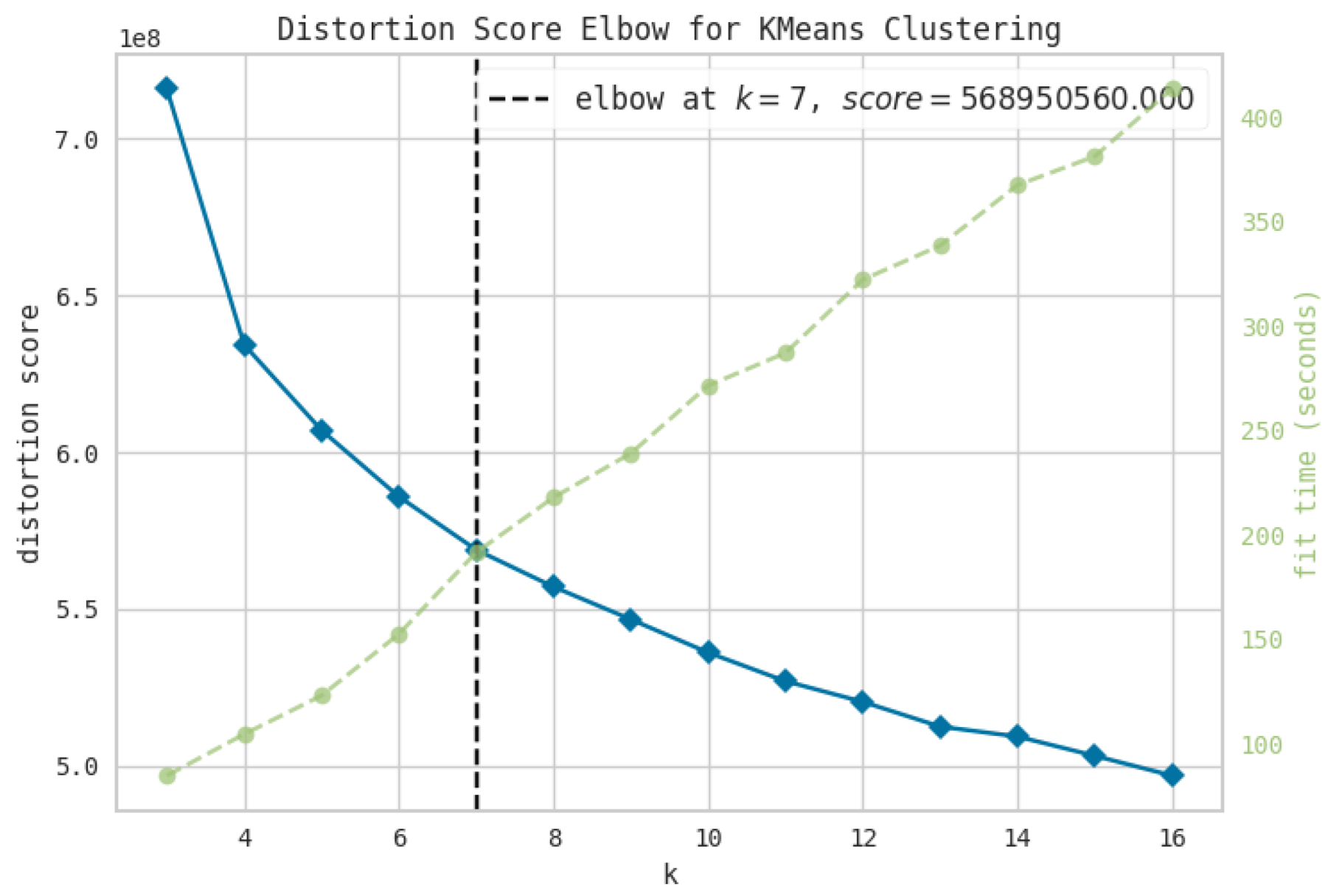
Elbow method suggests that an appropriate number of clusters is 7. However, qualitative analysis shows that these clusters have too much variation towards the edges. We will also see this with DBSCAN, although to a lesser degree. Nevertheless, the appropriate number of clusters according to the shilouette analysis is 5. Indeed, qualitatively speaking, using 5 clusters with k-means seems to make more sense. We can also observe this in the figure with TSNE, where using 5 clusters gives a clear separation, while using more than that results in more convolouted and intersected clusters. The main categories displayed by this clustering, are the ones most visually distinct that will come up later in any of the attempts to find different clustering. These are:
- Mostly normal pouring sequences.
- Mostly normal pouring sequences, but a tube occludes part of the stream, the mould is big.
- Mostly normal pouring sequences, but a tube occludes part of the stream, the mould is small.
- Light overflow which is promptly re-absorbed.
Figure 17.
Shilouette test. Shilouette score inducating the number of samples properly assigned to a cluster. The shilouette method suggests 5 as the number of cluster that has a better trade-off to represent the data.
Figure 17.
Shilouette test. Shilouette score inducating the number of samples properly assigned to a cluster. The shilouette method suggests 5 as the number of cluster that has a better trade-off to represent the data.
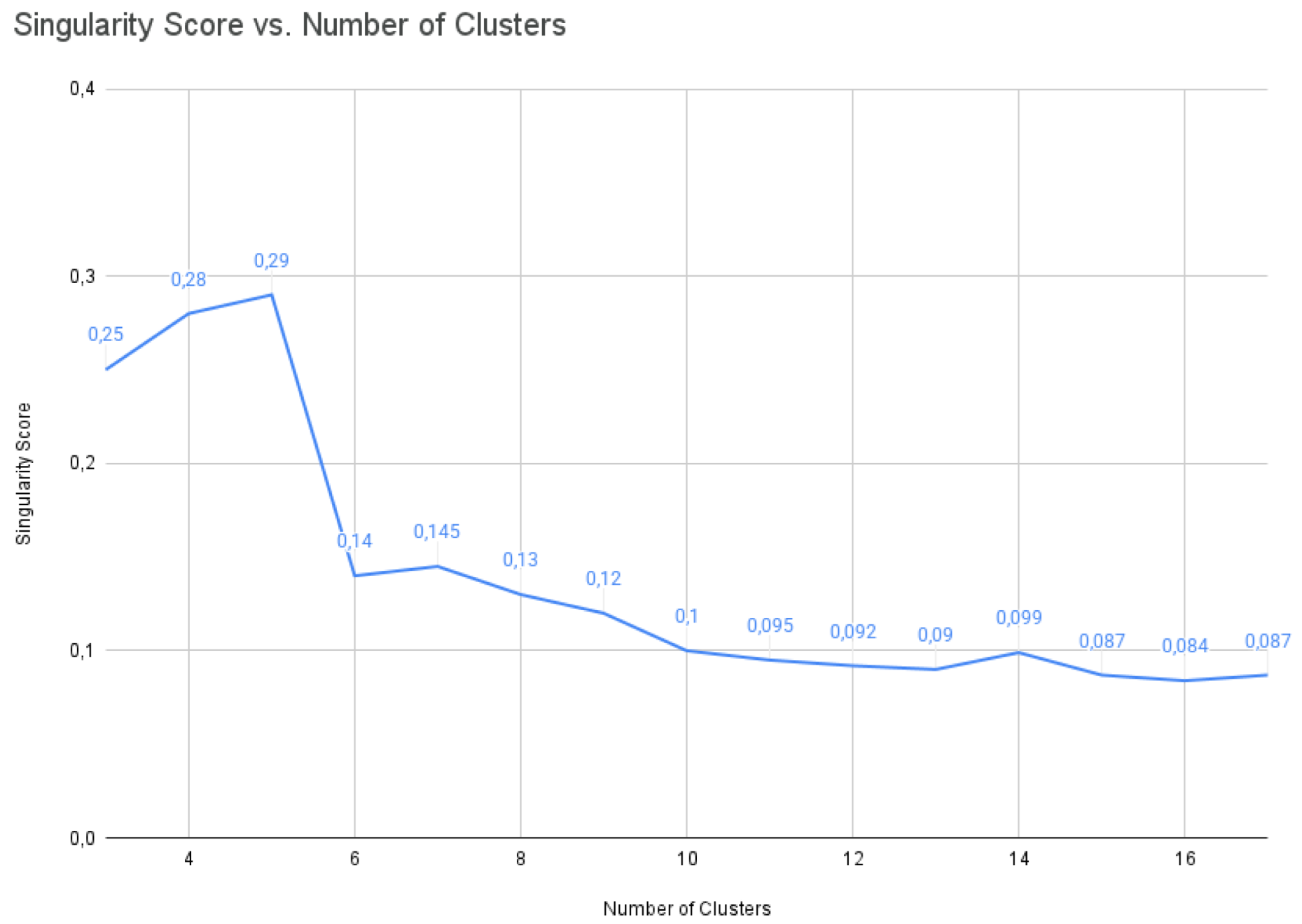
As we will also see later, these clusters tend to have more normal sequences towards the center of the cluster whereas they become un-naturalized (i.e., anomalies) with regards to that cluster as they approach the edge. This would require setting up a threshold distance to the centroid from which sequences start being considered anomalous, which is not so clear cut. However, this approach would require furhter analysis as these anomalous events near the edge are not straightforward to separate.
With K-means, as we increase the number of clusters, we observe that these four categories are split into multiple clusters which are difficult to differentiate qualitatively. This can be clearly seen in Figure 18, where results for k=5 and k=7 are shown. In the 2D visualization (Figures 18(a) and 18(b)), many clusters appear that seem to be splitting unnecessarily a single one into more than two when using , as the algorithm attempts an even distribution of samples across clusters. In the 3D visualization (Figures 18(c) and 18(d)), it is easy to see how many clusters seem to overlap, having samples within neighboring clusters. This explains the lower shilouette score.
DBSCAN: and min_samples
Different from K-Means, DBSCAN uses density to assess if samples should be included into a cluster, allowing for clusters of different density. This is controlled by two key parameters: and min_samples. The former controls the maximum distance up to which neighboring samples are considered. The latter controls how many of those neighbours need to pertain to a given cluster for the current sample to be classified into that cluster. Intuitively, denser regions will form the center of a cluster, as samples reinforce each other pertaining to specific clusters, whereas edge regions will have not enough samples, thus leaving outlier samples outside the given cluster. We find this feature of DBSCAN very useful for our use case, where finding anomalous instances is needed.
To find an appropriate , we first compute a pairwise distance matrix between all encoded video sequences (with the plain visual features). Through empirical tests, we find the mean distance (356) minus the standard deviation of the distances (85) represents the ceiling for the reasonable to be used, i.e., 270. Finding the proper value for is not straightforward, as there is a fine interplay with min_samples.
Using too big of a distance (i.e., ), allows too many samples to be clustered together. In all our experiments with this setting, around 60% of samples are clustered together into one cluster and around 30% into a secondary one. Both of them contain what, under inspection, we consider to be normal samples. Very few samples get clustered into one or two more very small clusters, as well as grouped as outliers. However, as we detail later, we find these to be of not much semantical significance. The main problem we observe with this bigger is that not many samples fall outside into the outlier group, which complicates the identification of anomalous samples.
When is small (i.e., ) it causes the algorithm to be more sensible to the choice of min_samples. Using min_samples results in many very small clusters (with samples), as they cannot get clustered with enough nearby samples (see Figure 19(b)). This phenomenon is driven by the interaction between these two parameters, but also by the high similarity between overlapping video sequences, which provides sufficient local density to meet the clustering criteria despite the lack of broader statistical significance. These clusters are often hyper-specific to particular video segments and do not represent generalized anomalous behavior. Nonetheless, in some cases we did find examples where very canonical anomalies appeared, which helped us identify the kind of outliers we had included in our dataset. In fact, as we increase min_samples for a given we also observe an increase of the samples that get no cluster assigned (i.e., they fall in the outlier cluster, see Figure 19(a)) This becomes increasingly evident with low values. We believe that these small clusters are not allowed to form, and instead, those samples are categorized as either anomalous or normal in the bigger clusters. These clusters, despite them being too small and overly-specific, seem to indicate that VideoMAE es capable of producing features that put these sequences together, allowing for such fine-grained categorization. Nevertheless, we believe that properly finding these clusters would require a more fine-grained hyper-parameter search for the clustering algorithm.
A small and small min_samples require denser areas to form clusters. On the one hand, with a small it is harder to find enough neighboring samples such that the min_samples requisite is met, resulting in more outlier samples. On the other hand, as a small min_samples allow for inclusion in a cluster with just a few samples, this results in many overly small clusters. As is increased, more distant samples are considered (those assigned to bigger clusters), resulting in those samples being clustered together and reducing the amount of small clusters. And as min_samples is increased, more neighbors of a given cluster are needed to categorize a sample into said cluster, making most of those samples in less dense areas to end up classified as outliers. Overall, and as it can be seen in Figure 19 for a given , increasing min_samples will result in less smaller clusters and more outlier samples. But for a given min_samples, increasing will result in less outlier samples and less smaller clusters.
Figure 20.
Number of samples on the four more stable bigger clusters found by DBSCAN for vision only features across various parameters combination for and min_samples.
Figure 20.
Number of samples on the four more stable bigger clusters found by DBSCAN for vision only features across various parameters combination for and min_samples.
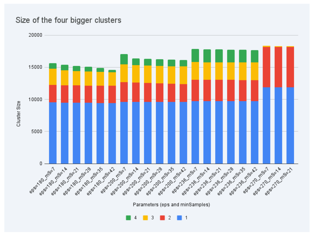
In general, we observe the formation of four more or less stable clusters, that qualitatively are equivalent to the ones described when discussing the results with KMeans: 1) Normal pouring events, 2 & 3) Normal pouring events with a tube in front of the frame (with both big and small mould), and 4) Slight overflow promptly reabsorbed. These are consistent over almost all combinations of parameters tested, failing to form only in cases where either is too big, or min_samples is large when is small. The first is generally the bigger cluster which is more stable regardless of the values of the two parameters, getting almost half the sequences. The next two are commonly the same size, adding up together up to a third of the sequences. The fourth and final cluster is the more variable, ranging from ∼800 samples up to ∼2000. In this regard, we observe that the smaller the value of , the more sensible the results are to the choice of min_samples. For example, for we can barely observe any difference in the results when varying min_samples.
Qualitatively speaking, we find two main types of anomalies. On the one hand, expected anomalies which are known to cause potential casting defects, most of them are shown in Figure 21. These events are closely related to common defects observed in continuous casting, such as incomplete mold filling, improper nucleation resulting in coarse microstructures, segregation phenomena, thermal cracking, and surface or internal defects like inclusions and porosity. Other than that, we also observe examples where the stopper was moving while pouring was active. On the other hand, the algorithm also finds anomalous samples which can be explained by sampling errors or by not properly detecting the pouring event/position. These are shown in Figure 22. As samples were shown in smaller 16-frame sequences, this also includes the least common beginning and end of pouring events, as they include some frames where no pouring occurs, and are sometimes wrongly categorized as outliers. We also find that samples where the mould is moving, which is normal behaviour outside of pouring, but it is categorized as outlier as not many sequences include it.
Although we believe none of the found combinations is perfect, as it still includes anomalous samples in the border of the normal clusters, and further cleaning is still possible. This could be achieved with the use of some hierarchical alternative such as HDBSCAN, the various analysis performed through different combinations of DBSCAN parameters have allowed us to identify expected types of anomalies as well as others that may as well be due to sampling or data pre-processing issues. We believe our current approach offers very promising results, showing the separability of normal and anomalous samples in industrial scenarios. The preliminary results obtained here will allow us to perform a second iteration with the human in the loop, where pouring experts can annotate only a subset of the sequences, based on the results obtained here, reducing the annotation burden by being able to remove more than half of the sequences that we can surely assess are normal.
Multimodality
Figure 23.
Number of samples on the four more stable bigger clusters found by DBSCAN for multimodal features across various parameters combination for and min_samples.
Figure 23.
Number of samples on the four more stable bigger clusters found by DBSCAN for multimodal features across various parameters combination for and min_samples.
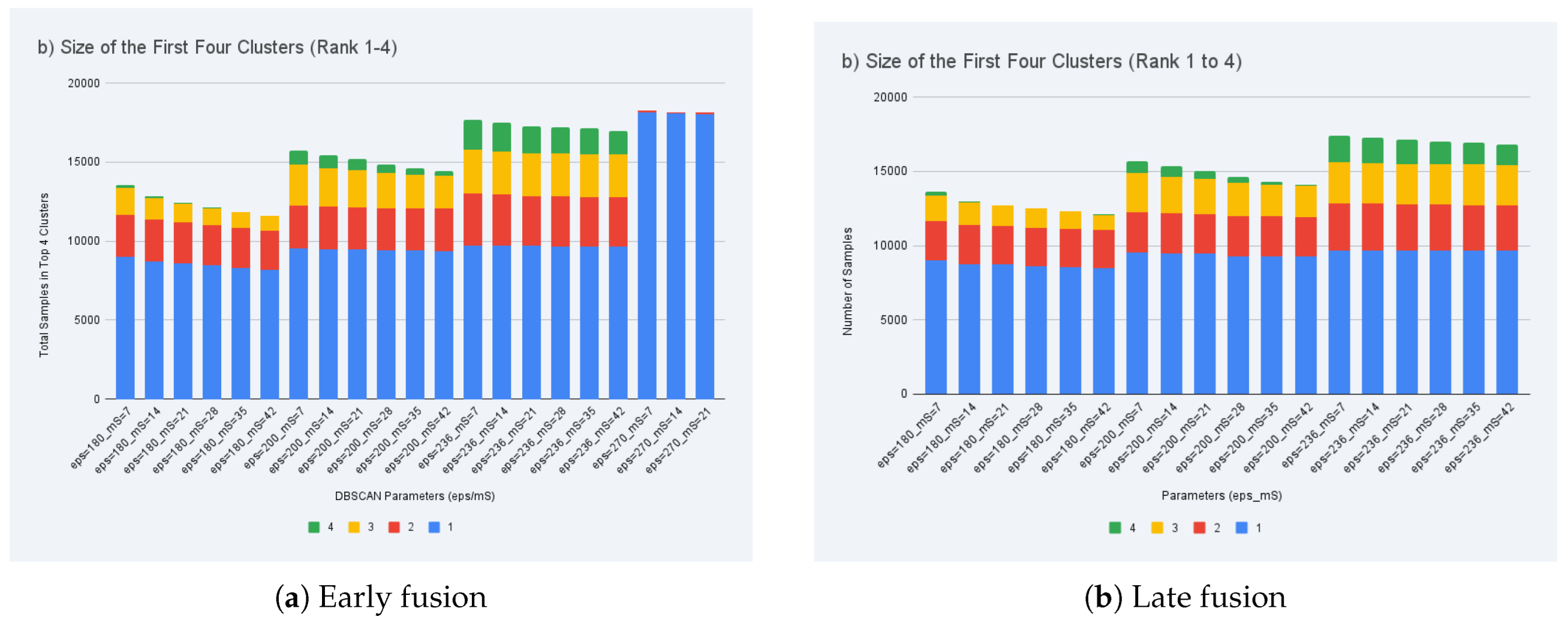
We have not been able to find substantial differences when using sensory data. We tested both, early and late fusion, with no notable differences between them. Nonetheless, we do tend to find more outlier samples, both in terms of number of samples in the main outlier cluster, as well as in terms of number of very small cluster containing hyper-specific categories. This could be related to being fixed through the average distance between sequences computed for the vision-only features. This causes that, for very small we find a reduction in the number of samples that fall inside the four big normality clusters, and instead end up in either the outlier group or the very small clusters. This results on the reduction of anomalous samples towards the edges of the clusters. Nonetheless, the excess of small clusters, specially with small , which can either display normal or anomalous samples, further complicates the final regression of the anomalous score, thus there is not a clear benefit of this finding. Normality tends to be concentrated in the bigger clusters with higher intra-similarity, and spreading anomalies like that may be counter-productive.
Figure 24.
Number of samples left as outliers by DBSCAN across various parameters combination for and min_samples.
Figure 24.
Number of samples left as outliers by DBSCAN across various parameters combination for and min_samples.
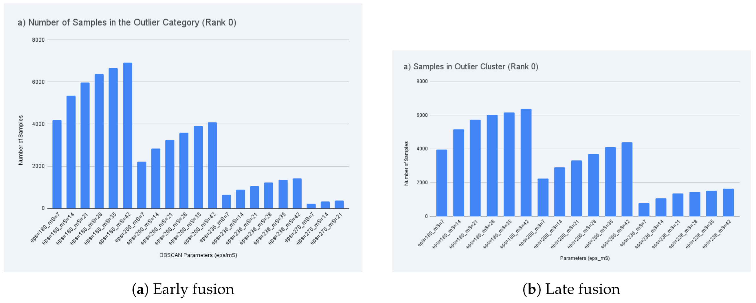
Another difference is when using eps=270. In the case of using sensory inormation, the whole dataset (except very few outliers, ∼300) fall into a single cluster. On the contrary, when only using visual information we get two main clusters, one with most of the sequences (∼11K), and another with the tube occluding part of the stream (∼6K).
Finally, we believe this additional number of samples that fall outside of defined clusters may be explained by anomalies found exclusively on sensory data, which cannot be as easily observed as the ones explained visually. In this regard, some of the anomalies found could be either sensory anomalies or, alternatively, noisy values of the sensors. Nonetheless, this shows successful integration of the sensory data, as it is clearly being used by the clustering algorithm to find anomalous samples.
Agreement
To compute the final score for a given pouring event we use the percentage of sequences from that pouring event which get assigned to no cluster, resulting on a value from 0 to 1. We set up a threshold of 0.6 to consider a pouring event as anomalous, but for the final MoE we use the continuous value instead.
From ground truth information provided by the factory where our data came from, we know that ∼3% of the moulds are rejected because of defects that originated by some fault related to the pouring. In this sense, from the 539 detected moulds detailed in Table 2, we identify 549 pouring events, from which we should expect to find ∼16 that are anomalous. However, as we saw above, our system currently also finds anomalies that were caused by a sampling problem, and not due to actual pouring problems. In this sense, we consider that 16 should be taken as a lower bound.
In Figure 25 we show the distribution of the number of detected anomalous pouring events using a threshold of 0.6 to the anomaly score. As it can be seen, only multimodal variants are capable of retrieving a number of sequences consistent with expert knowledge about defects on casting pouring. Qualitative analysis for the model variants using and min_samples reveals that 60% of the pouring events marked as anomalous indeed show expected anomalies (see Figure 21), 20% of them can be attributed to sampling errors (see Figure 22), and the remaining sequences appear to be normal, but we believe they were classified as anomalies due to sensory information which is more complex to quantify. Overall, we find that the model variants in this range represent good candidates for a first filtering step that eases manual annotation and clearly separates the normal sequences from potential anomalies.
3.5. Mixture of Experts
The manufacturing evaluation stage operates on the set of pouring events successfully detected by the vision pipeline. For this evaluation, we considered the 539 pouring events correctly detected and reported in Table 2. For each detected pouring event , we computed a set of temporal indicators, namely pouring duration , the inter pouring time , and the mould idle time . After excluding problematic cases with missing or unreliable measurements, these variables exhibit a stable and narrow distribution across regular production cycles. The average pouring duration is approximately , with moderate dispersion, while idle times remain consistently within the expected operational range. Only a small fraction of events shows deviations in , typically correlated with context states such as short stoppages or maintenance actions identified by the global context classifier. Regarding the visual evaluation of the pouring stream, most events present a single continuous segment, corresponding to uninterrupted pouring. In fact, stream interruptions, quantified by the variable , are observed in a limited subset of events and usually occur near the beginning or end of the pouring interval. Such cases are often associated with transient instabilities or borderline visual conditions rather than systematic failures.
In summary, the manufacturing evaluation stage focuses on extracting, validating and structuring heterogeneous indicators describing each pouring cycle, including visual states, temporal measurements and process-level constraints. At this point, all variables are preserved as independent evidences, without enforcing a final quality decision. The joint interpretation of these indicators, together with the domain specific rules and contextual information, is managed in the next stage through a Mixture-of-Experts architecture. This MoE based unification enables the transformation of the measured evidence into a coherent and high-level assessment suitable for a third-party integration, for instance, with a digital twin and supervisory decision making system.
3.5.1. MoE Unification and Digital Twin
The previous stages provide complementary, but still independent, observations of each pouring cycle: (i) the temporal delimitation of pouring events, (ii) the localisation of key AoIs, and (iii) the frame-level interpretation of stream and mould states. The role of the present layer is to convert this heterogeneous set of evidences into a single event-centred representation that can be queried, stored, and acted upon at line speed. Rather than performing additional vision processing, the focus is on evidence fusion. Actually, it is centered on combining temporal variables, geometric cues, and semantic labels into a coherent assessment of each pouring cycle, enabling traceability, early quality screening, and real-time interoperability with supervisory and digital twin platforms.
Event Centered Data Model
Each mould cycle is represented as a POURING_EVENT record indexed by the event window (see Section 2.3.1). Specifically, the record stores several information such as (i) the event timing (, , ), (ii) the local interpretation of the scene (i.e., anomalous status , number of cuts , mould filling state , tile presence and incoming warning flag ), and (iii) the operational context segments coming from the global environment evaluator.
Since movement based event identification is affected by occlusions and maintenance operations, the final population of events must be interpreted together with the detection statistics already reported in Table 2.
Sanity checks and temporal consistency
Before the process of merging the information, the MoE layer applies a lightweight validation. In fact, it is the step to ensure that the recorded event is temporally coherent:
Hence, events that fail these constraints are still stored for traceability. Nevertheless, they are identified as non-assessable and they are also excluded from the strict quality calculation or scoring. This is particularly relevant in borderline sequences where operator occlusions, technical stops, or partial visibility of the conveyor can disturb the motion signal or the AoI evaluation.
MoE Structure and Decision Logic
Then, when all information is interpreted, the MoE is the place where each expert set of features are handled to finally produce an interpretable classification of the pouring event following the expert combination explained below.
- Temporal expert: evaluates the correctness of the event comparing the temporal information with each reference control plan limits using , , and .
- Stream expert: interprets and (cuts), penalising unstable or interrupted flows.
- Cup expert: aggregates the tracked filling states (and the incoming warning flag ) to detect spill, underfill, and premature splashes.
- Context expert: reduces the influence of evidence during non-regular operating periods (e.g., maintenance or stoppages), retaining it for traceability while avoiding spurious quality alarms.
All those expert outputs are fused by a gating function that is explicitly conditioned on context. Operationally, the MoE produces (a) a discrete label and (b) an explanation vector with the dominant contributing factors (e.g. cut detected, overflow warning, out-of-limit pour duration, maintenance segment present).
Observed statistics from the event records and MoE decision summary
For evaluating this work, we have employed the same one hour run that it was used before. In that way, the parsed POURING_EVENT logs show that most cycles are temporally stable (explained below in Table 4), with a tight inter-pour rhythm and occasional outliers caused by operational interruptions. The average number of stream interruptions is low. In fact, only 5.38% of events contain at least one cut (i.e. ), indicating that discontinuous flows are sporadic rather than systematic.
Furthermore, the status flags calculated indicate that the majority of events are considered OK by the upstream checks, with a smaller fraction requiring review due to minor inconsistencies, such as short partial segments or atypical timing under occlusions. These flags are used by the MoE as priors rather than final decisions, since the ultimate quality label is produced after the multi-source fusion process.
After aggregating all validated evidences at event level, the MoE module assigns a final operational decision to each detected pouring cycle. This decision reflects the joint evaluation of temporal compliance, stream stability, mould filling conditions, and operational context. Events flagged as non-assessable due to partial visibility or external disturbances are excluded from strict quality scoring but preserved for traceability.
Table 5 summarises the distribution of MoE decisions obtained from the selected one hour evaluation video.
From a validation perspective, a full mould-by-mould correlation between the MoE decisions and the final casting quality is not feasible at this stage. This limitation is mainly due to the lack of part-level traceability between individual pouring events and downstream defect inspection, as well as the presence of external disturbances affecting both detection and quality assessment. Consequently, the evaluation strategy adopted in this work relies on a comparison at the production statistics level, which is a common and accepted practice in industrial foundry environments.
Specifically, the overall defect rates provided by the foundry, together with the proportion of defects explicitly associated with pouring related phenomena, are contrasted with the distribution of MoE decision outcomes obtained over the same production interval. According to the plant quality records, the total rejection rate during the analysed period is . Among these rejected parts, approximately correspond to defect types directly linked to the pouring stage. These results in an effective pouring related defect rate is approximately:
During the same one hour production video and based on the pouring related defect rate, approximately 17 moulds would be expected to present quality issues related to pouring anomalies within this time interval. Consequently, and taking into account the values shown in Table 5, the overall anomaly detection rate of the system, defined as the union of Review and Not_OK events, is:
In that way, and comparing with the estimated of pouring related defects reported by the foundry, the system exhibits a close correspondence in terms of order of magnitude. The slight overestimation observed in the MoE anomaly rate can be reasonably attributed to two factors: (i) the conservative nature of the supervisory strategy, which prioritises early risk detection over missed defects, and (ii) the residual detection error inherent to vision-based mould identification under real industrial conditions. Importantly, the system does not under detect potentially defective events, which is a critical requirement for quality assurance and process supervision.
Causal Analysis and Explainability of MoE Decisions
Beyond the final decision counts, the MoE architecture enables analysing which groups of indicators predominantly contributed to each decision category. Decisions do not rely on a single expert, but rather emerge from the weighted combination of multiple evidences, including temporal compliance, pouring stream behaviour, mould filling states, and operational context.
Table 6 summarises the dominant contributing factors associated with each MoE output class.
One of the main advantages of the proposed MoE architecture is that each decision can be traced back to a limited set of contributing experts and variables. Instead of producing a single opaque score, the system preserves the individual expert outputs and their relative influence on the final decision.

Table 7.
Most influential indicators contributing to MoE decisions, grouped by expert domain.
| Expert domain | Indicator | Interpretation in MoE decision |
|---|---|---|
| Pouring stream expert | , | Stream class and number of interruptions strongly influence Review and Not_OK outcomes when instability or cuts are detected. |
| Temporal expert | , | Deviations from reference time windows contribute to risk escalation, especially under repeated or combined violations. |
| Mould filling expert | Incorrect filling states provide early evidence of material loss, while overpouring contributes as a warning signal rather than an immediate rejection. | |
| Safety and protection expert | , tile presence | Incoming mould warnings and absence of protective elements act as safety-driven penalties within the MoE. |
| Context expert | Non-regular operational contexts modulate decision confidence and may downgrade events to Review rather than Not_OK. |
Integration with the Digital Twin and supervisory systems.
Once the MoE decision is produced for each pouring event, the resulting assessment is exposed to higher-level systems through a structured and machine-readable interface. Each evaluated event is encoded as a JSON object aggregating raw measurements, intermediate expert outputs, and the final MoE decision, preserving full traceability of the reasoning process.
This information is streamed in real time via a WebSocket communication layer to the digital twin of the foundry process. Rather than receiving a binary quality flag, the digital twin ingests a semantically rich representation including temporal metrics, pouring stream descriptors, mould filling states, safety indicators, and contextual annotations. This enables synchronisation of the physical and virtual processes at event level, supporting advanced monitoring, replay, and causal analysis.
Overall, the MoE unification stage acts as the semantic bridge between low-level visual perception and high-level manufacturing intelligence. By combining heterogeneous evidences into an explainable and structured decision, the system enables consistent quality assessment while maintaining interpretability and traceability at event level.
4. Discussion and Conclusion
This work addresses a critical industrial challenge in iron foundries, specifically, the reliable monitoring and interpretation of pouring operations. This stage is particularly critical, as a significant proportion of casting defects originate during pouring are subsequently propagated downstream throughout the production process. This kind of pouring related anomalies, such as incomplete filling, cold shuts, and metal losses directly compromise the final casting quality, operational safety, and overall production efficiency. Despite its importance, the pouring process remains difficult to supervise consistently under real industrial conditions due to its harsh environment and dynamic nature. To handle this challenge, the proposed framework integrates multimodal perception, temporal reasoning, and expert-based decision logic into a unified and explainable system, enabling robust monitoring and interpretation of pouring operations in industrial foundries. The main contribution of this research lies in demonstrating that heterogeneous sources of evidence (i.e., visual, temporal, and contextual) can be effectively unified into a coherent operational assessment of each pouring cycle. Rather than focusing on isolated detections or individual indicators, the proposed system transforms raw observations into structured and interpretable representations that capture both process behaviour and compliance with the foundry control plan. Accordingly, the experimental results demonstrate that individual pouring events can be reliably segmented. Moreover, key AoIs can be detected and tracked, and meaningful indicators describing stream stability, filling quality, and safety conditions can be consistently extracted. When the objectives outlined in Section 1 are considered in an unified way, the obtained results confirm that the proposed approach fulfils its intended scope. Thus, pouring events are robustly identified under real production conditions, and the critical visual elements required to interpret pouring dynamics are detected with high reliability. On this basis, interpretable indicators are consistently derived to characterise stream behaviour, mould filling states, and temporal compliance. In addition, heterogeneous sources of evidence are unified through an explainable MoE architecture, enabling a coherent and event centred operational assessment. Building upon this capability, the statistical evaluation of the system behaviour provides consistent evidence that the proposed MoE framework captures the underlying defect generation mechanisms of the pouring process. Events flagged as Review or Not_OK are predominantly associated with conditions known to increase defect probability, such as stream interruptions, turbulence, abnormal filling states, or temporal deviations from the control plan. Conversely, events classified as OK correspond mainly to stable and compliant pouring cycles. Consequently, any residual discrepancies between the system outputs and production statistics define a clear and actionable pathway for future refinements, including threshold tuning, expert weighting adjustments, and the incorporation of additional sensing modalities.
One of our core novel contributions regards the identification of anomalous pouring streams. We have presented a novel framework for anomaly detection in complex industrial scenarios, specifically targeting molten metal pouring processes. By leveraging a multi-modal sensor fusion strategy, we successfully integrated video data with disparate sensory readings through a self-supervised learning objective. To the best of our knowledge, this represents one of the first applications of VideoMAE transformers for industrial outlier detection. Our approach demonstrates that learning jet stream dynamics via reconstruction, followed by density-based clustering, offers a robust alternative to traditional supervised methods, which are often hampered by the scarcity of defective samples in manufacturing environments. Our extensive experimental analysis highlights the superior suitability of density-based clustering, specifically DBSCAN, over partition-based methods like K-Means for this domain. While K-Means forces data into rigid partitions, DBSCAN naturally isolates outliers, aligning better with the definition of industrial anomalies. We observed the consistent formation of four primary “normal” clusters—representing standard pouring, occlusion variations, and minor reabsorbed overflows—regardless of the modality used. This stability suggests that the visual features, which constitute approximately 90% of the feature space, dominate the representation. However, the integration of sensory information proved crucial; while vision defined the structural clusters, the multi-modal variants identified a higher number of anomalous samples that aligned more closely with the expected defect rates (∼3%), capturing irregularities likely invisible to the naked eye. Despite these successes, the definition of an anomaly remains a nuanced challenge. We observed that while distinct outliers are easily flagged, many samples exist on the “edges” of normal clusters, exhibiting increasing deviation from the centroid. Currently, the boundary between a “noisy normal” sample and a “subtle anomaly” is dictated by the hyperparameters and min_samples, which can be sensitive to tune. Therefore, we posit that this method is not yet a replacement for human expertise but rather a powerful augmentation tool. By successfully filtering the vast majority of normal operation data, our system significantly alleviates the annotation burden, allowing human experts to focus their attention on verifying a targeted subset of potential defects.
Finally, the generation of structured and machine-readable outputs ensures direct compatibility with digital twin and supervisory platforms. This capability bridges the gap between low-level perception and higher-level industrial decision-making systems, allowing the extracted knowledge to be consumed, contextualised, and exploited beyond isolated detection tasks. A key strength of the proposed MoE architecture is its explainability. Instead of collapsing all observations into a single opaque score, the system preserves individual expert outputs and their relative influence on the final decision. This property enables causal analysis of OK, Review, and Not_OK outcomes and facilitates alignment with expert judgement. In addition, qualitative assessment performed together with foundry specialists confirms that the decisions are consistent with domain knowledge, particularly in distinguishing stable production from borderline or potentially risky conditions. Importantly, situations such as mild overflow are correctly interpreted as warning-level events rather than obvious errors, reflecting realistic industrial practice.
Despite the promising results achieved in our research work, the proposed framework exhibits several limitations that must be critically analysed to properly contextualise its applicability and guide future developments. These limitations are not specific to the proposed architecture but are representative of current challenges in industrial vision-based monitoring systems.
The first limitation concerns the dependency on visual acquisition conditions. Hence, although the detection and tracking modules demonstrated robust behaviour under normal production scenarios, performance degradation may occur under non-ideal illumination (i.e., intense glare from molten metal, smoke, or partial occlusions caused by operators or maintenance activities). These similar constraints have been reported in other vision-based foundry monitoring systems, where illumination variability and environmental noise remain major sources of uncertainty [12,13]. To solve this problems, recent studies suggest that integrating complementary modalities such as thermal imaging or multispectral sensing can mitigate these effects by providing illumination invariant cues [117,118]. Consequently, incorporating these modalities into the proposed multimodal framework represents a natural and well founded extension.
The second detected limitation relates to the representation of rare but critical pouring anomalies. In other words, events such as severe nozzle clogging, abrupt ladle misalignment, or extreme overflows occur infrequently in normal production although they have a disproportionate impact on quality and safety. As a result, they are underrepresented in the available training data, limiting the learning capacity of data-driven components. This issue has been widely recognised in industrial anomaly detection literature [113]. Hence, there are some works in the bibliography that try to face this challenge using synthetic data generation, physics-based simulation, or generative models to augment this type of samples [8,119]. Ergo, applying similar strategies to pouring dynamics would allow the MoE system to better generalise its behaviour.
Another important limitation concerns the long term stability of sensor derived indicators and temporal measurements. The current implementation assumes properly calibrated sensors and stable acquisition conditions. Nevertheless, sensor drift, mechanical wear, and changes in production references over time can progressively degrade the reliability of temporal indicators such as pouring duration or inter pouring intervals. This challenge has been extensively discussed in fault diagnosis and condition monitoring literature [10,14]. In that way, adaptive thresholding strategies, online recalibration mechanisms, and self-supervised drift detection techniques have been proposed to maintain robustness [120]. These approaches could be integrated into the temporal expert of the proposed MoE architecture without altering its overall structure.
Regarding detecting anomalous pouring events, we believe the process could benefit from improved granularity of detection. A primary focus should be a deeper analysis of intra-cluster distances. We hypothesize that the Euclidean distance of a sample to its cluster centroid could serve as a continuous “anomaly score”, providing a soft filtering mechanism for edge cases that DBSCAN currently classifies strictly as binary noise or inliers. Furthermore, to better address the sensitivity of global hyperparameters, we intend to explore hierarchical clustering algorithms, such as HDBSCAN, or iterative sub-clustering strategies. These approaches could dynamically adapt to the varying densities of different operational modes, potentially separating the "edge" regions more effectively than a global density threshold. Additionally, the role of sensory data warrants further investigation. Our results showed that multi-modal models flagged samples that appeared visually normal as anomalous, suggesting the sensors captured latent process deviations. Future work should pursue a rigorous correlation analysis of these specific samples against downstream quality control logs to validate the physical nature of these "invisible" defects. Furthermore, we envision the immediate next step as the deployment of this system in an iterative, human-in-the-loop framework. by presenting the detected outliers to factory experts, we can not only validate the system’s current precision but also use expert feedback to progressively refine the feature space, moving from unsupervised exploration toward a robust, semi-supervised anomaly detection pipeline.
From the decision making perspective, although the MoE framework provides explainable and modular reasoning, the current rule-based aggregation relies on defined thresholds and weighting strategies by foundry experts. While this ensures transparency and alignment with foundry knowledge, it may limit adaptability across different production lines or alloy families. Hence, hybrid approaches that combine expert rules with learnable gating mechanisms have been shown to preserve interpretability while improving adaptability [121,122]. Thus, the introduction of partially learnable activation functions, constrained by expert-defined priors, is a promising direction for improving scalability without sacrificing explainability.
Finally, the current research work does not yet close the loop between perception and control. Although the structured JSON outputs are designed for digital twin integration, the system currently operates in an observational and supervisory mode. Several recent industrial digital twin implementations demonstrate that closing this loop can significantly improve process stability and reduce defect rates [112,123]. Hence, deploying the proposed framework within an online digital twin ecosystem would enable not only real-time monitoring but also predictive scenario evaluation and corrective action recommendation.
In conclusion, this work demonstrates that an explainable, multimodal MoE based framework provides a robust and industrially meaningful solution for supervising pouring operations in iron foundries. By unifying visual perception, temporal analysis, and domain-driven expert knowledge into a coherent decision layer, the proposed approach advances the state of the art in pouring monitoring while delivering interpretable outputs aligned with real production constraints. At the same time, the identified limitations do not weaken the validity of the proposed system; instead, they define a clear and realistic roadmap for its evolution. Hence, future extensions will progressively incorporate additional sensing modalities, rare event augmentation strategies, adaptive temporal modelling, and tighter online integration with digital twin infrastructures, enabling the framework to mature towards a fully autonomous, resilient, and scalable solution for intelligent pouring supervision and data-driven foundry operations.
Author Contributions
Conceptualization, J.N. and J.S.; methodology, J.N. and J.S.; software, J.N. and J.S.; validation, J.N., J.S. and F.A.S.; formal analysis, J.N., J.S., G. E.-R., J. A.-P., J. L. and X. B.; investigation, J.N., J.S., G. E.-R., J. A.-P., J. L. and X. B.; resources, J.N. and J.S.; data curation, J.N., J.S., G. E.-R., J. A.-P., J. L. and X. B.; writing—original draft preparation, J.N. and J.S.; writing—review and editing, J.N., J.S. and F.A.S.; visualization, J.N. and J.S.; supervision, J.N., J.S. and F.A.S.; project administration, J.N. and F.A.S.; funding acquisition, J.N. and F.A.S. All authors have read and agreed to the published version of the manuscript.
Funding
This research work was funded by the Elkartek Programme (Basque Government) for the IKUN project (grant number KK-2024/00064). The views and opinions expressed are solely those of the authors and do not necessarily reflect those of the Basque Government, nor can the Basque Government be held responsible for them.
Institutional Review Board Statement
Not applicable.
Informed Consent Statement
Not applicable.
Data Availability Statement
The dataset (i.e., videos and signals) used in this study was compiled from an specific foundry. Due to the confidential nature of the data and the proprietary knowledge it reflects regarding specific manufacturing processes, the dataset cannot be shared. Nonetheless, the authors have made every effort to thoroughly document the methodology and the tools developed, enabling other researchers or practitioners to reproduce a similar solution using their own data.
Conflicts of Interest
The authors declare no conflicts of interest.
Appendix A. JSON File Example
A representative example of the JSON-based structure to be transmitted to the downstream digital twin.
{
"start_time": 0,
"end_time": 20.52,
"cycle_time": "20.52s",
"idle_time": "7.44s",
"idle_time_ok": false,
"inter_pouring_time": "8.88s",
"inter_pouring_time_ok": true,
"pouring_time": "10.32s",
"pouring_time_average": 7.08,
"pouring_during_movement": false,
"status": "REVIEW",
"anomalous_score": 0.4,
"pouring_comments": "Idle time exceeded.",
"pouring_segments": [
{"start_time": "6.96s", "end_time": "17.28s", "duration": "10.32s"}
],
"environment_status_segments": [
{
"start_time": "0.16s",
"end_time": "0.72s",
"duration": "0.56s",
"status_value": "Normal"
},
{
"start_time": "0.72s",
"end_time": "7.12s",
"duration": "6.40s",
"status_value": "Stopline"
},
{
"start_time": "7.12s",
"end_time": "20.64s",
"duration": "13.52s",
"status_value": "Normal"
}
]
}
References
- Market Growth Reports. Iron Casting Market Size & Industry Analysis 2035, 2025. Accessed 2025-01-07.
- ASM International. ASM Handbook, Volume 1A: Cast Iron Science and Technology; ASM International, 2017.
- Nian, Y.; Zhang, L.; Zhang, C.; Ali, N.; Chu, J.; Li, J.; Liu, X. Application status and development trend of continuous casting reduction technology: A review. Processes 2022, 10, 2669.
- Salonitis, K.; Zeng, B.; Mehrabi, H.A.; Jolly, M. The challenges for energy efficient casting processes. Procedia Cirp 2016, 40, 24–29.
- Patel, V.D.; Patel, U.J.; Patel, V.P.; Patel, V. Review of Casting Processes, Defects and Design. International Journal for Research in Engineering Application & Management 2021, pp. 25454–9110.
- Jose, S.; Nguyen, K.T.; Medjaher, K. Enhancing industrial prognostic accuracy in noisy and missing data context: Assessing multimodal learning performance. Journal of Intelligent Manufacturing 2024, pp. 1–25.
- Sheng, Y.; Zhang, G.; Zhang, Y.; Luo, M.; Pang, Y.; Wang, Q. A multimodal data sensing and feature learning-based self-adaptive hybrid approach for machining quality prediction. Advanced Engineering Informatics 2024, 59, 102324.
- Qu, X.; Liu, Z.; Wu, C.Q.; Hou, A.; Yin, X.; Chen, Z. Mfgan: multimodal fusion for industrial anomaly detection using attention-based autoencoder and generative adversarial network. Sensors 2024, 24, 637.
- Yan, W.; Wang, J.; Lu, S.; Zhou, M.; Peng, X. A review of real-time fault diagnosis methods for industrial smart manufacturing. Processes 2023, 11, 369.
- Leite, D.; Andrade, E.; Rativa, D.; Maciel, A.M. Fault Detection and Diagnosis in Industry 4.0: A Review on Challenges and Opportunities. Sensors (Basel, Switzerland) 2024, 25, 60.
- Popoola, N.T.; Bakare, F.A. Advanced computational forecasting techniques to strengthen risk prediction, pattern recognition, and compliance strategies 2024.
- Chen, M.C.; Yen, S.Y.; Lin, Y.F.; Tsai, M.Y.; Chuang, T.H. Intelligent Casting Quality Inspection Method Integrating Anomaly Detection and Semantic Segmentation. Machines 2025, 13, 317.
- Tao, X.; Gong, X.; Zhang, X.; Yan, S.; Adak, C. Deep learning for unsupervised anomaly localization in industrial images: A survey. IEEE Transactions on Instrumentation and Measurement 2022, 71, 1–21.
- Guo, S.; Sharif, J.M. Real-Time Temperature Prediction Model for Online Continuous Casting Control Using Simplified Boundary Condition Computing Method. Processes 2025, 13, 305.
- Lee, J.; Noh, S.D.; Kim, H.J.; Kang, Y.S. Implementation of Cyber-Physical Production Systems for Quality Prediction and Operation Control in Metal Casting. Sensors 2018, 18. [CrossRef]
- Nieves, J.; Bravo, B.; Sierra, D.C. A Smart Digital Twin to Stabilize Return Sand Temperature without Using Coolers. Metals 2022, 12. [CrossRef]
- Nieves, J.; Garcia, D.; Angulo-Pines, J.; Santos, F.; Rodriguez, P.P. An Artificial Intelligence-Based Digital Twin Approach for Rejection Rate and Mechanical Property Improvement in an Investment Casting Plant. Applied Sciences 2025, 15. [CrossRef]
- Tong, Z.; Song, Y.; Wang, J.; Wang, L. VideoMAE: Masked Autoencoders are Data-Efficient Learners for Self-Supervised Video Pre-Training. In Proceedings of the Advances in Neural Information Processing Systems; Koyejo, S.; Mohamed, S.; Agarwal, A.; Belgrave, D.; Cho, K.; Oh, A., Eds. Curran Associates, Inc., 2022, Vol. 35, pp. 10078–10093.
- Ester, M.; Kriegel, H.P.; Sander, J.; Xu, X.; et al. A density-based algorithm for discovering clusters in large spatial databases with noise. In Proceedings of the kdd, 1996, Vol. 96, pp. 226–231.
- Posner, E.A.; Spier, K.E.; Vermeule, A. Divide and conquer. Journal of Legal Analysis 2010, 2, 417–471.
- Mackey, L.; Jordan, M.; Talwalkar, A. Divide-and-conquer matrix factorization. Advances in neural information processing systems 2011, 24.
- Horowitz.; Zorat. Divide-and-conquer for parallel processing. IEEE Transactions on Computers 1983, 100, 582–585.
- Campbell, J. Complete Casting Handbook: Metal Casting Processes, Metallurgy, Techniques and Design, 2nd ed.; Butterworth-Heinemann: Oxford, UK, 2015.
- Beeley, P.R. Foundry Technology, 2nd ed.; Butterworth-Heinemann: Oxford, UK, 2001.
- ASM International. Casting. In ASM Handbook; ASM International: Materials Park, OH, USA, 2005; Vol. 15. See chapters on sand casting and process control.
- Banchhor, R.; Ganguly, S. Optimization in green sand casting process for efficient, economical and quality casting. Int J Adv Engg Tech 2014, 5, 29.
- Stefanescu, D.M. Science and Engineering of Casting Solidification, 3rd ed.; Springer: Cham, Switzerland, 2018.
- Askeland, D.R.; Wright, W.J. The science and engineering of materials; Cengage Learning, 2010.
- Rebouças, E.S.; Braga, A.M.; Marques, R.C.; Rebouças Filho, P.P. A new approach to calculate the nodule density of ductile cast iron graphite using a Level Set. Measurement 2016, 89, 316–321. [CrossRef]
- He, K.; Zhang, X.; Ren, S.; Sun, J. Deep residual learning for image recognition. Proc. IEEE Conf. Comput. Vis. Pattern Recognit. (CVPR) 2016, pp. 770–778.
- Tan, M.; Le, Q. Efficientnet: Rethinking model scaling for convolutional neural networks. In Proceedings of the International conference on machine learning. PMLR, 2019, pp. 6105–6114.
- Dosovitskiy, A. An image is worth 16x16 words: Transformers for image recognition at scale. arXiv preprint arXiv:2010.11929 2020.
- Liu, Z.; Mao, H.; Wu, C.Y.; Feichtenhofer, C.; Darrell, T.; Xie, S. A ConvNet for the 2020s, 2022, [arXiv:cs.CV/2201.03545].
- Ultralytics. Ultralytics YOLOv11 Documentation and Model Zoo. https://docs.ultralytics.com/models/yolo11/, 2024. Accessed: 29 October 2025.
- Zhang, Q.; Zhang, K.; Pan, K.; Huang, W. Image defect classification of surface mount technology welding based on the improved ResNet model. Journal of Engineering Research 2024, 12, 154–162.
- Chen, Q.; Xiong, Q.; Huang, H.; Tang, S.; Liu, Z. Research on the Construction of an Efficient and Lightweight Online Detection Method for Tiny Surface Defects through Model Compression and Knowledge Distillation. Electronics 2024, 13, 253.
- Feng, X.; Gao, X.; Luo, L. An improved vision transformer-based method for classifying surface defects in hot-rolled strip steel. In Proceedings of the Journal of Physics: Conference Series. IOP Publishing, 2021, Vol. 2082, p. 012016.
- Li, Z.; Yan, Y.; Wang, X.; Ge, Y.; Meng, L. A survey of deep learning for industrial visual anomaly detection. Artificial Intelligence Review 2025, 58, 279.
- Ouardirhi, Z.; Mahmoudi, S.A.; Zbakh, M. Enhancing Object Detection in Smart Video Surveillance: A Survey of Occlusion-Handling Approaches. Electronics 2024, 13. [CrossRef]
- Schäufele, J. Improved RAFT architectures for optical flow estimation. PhD thesis, Universität Stuttgart, 2021.
- Eslami, N.; Arefi, F.; Mansourian, A.M.; Kasaei, S. Rethinking raft for efficient optical flow. In Proceedings of the 2024 13th Iranian/3rd International Machine Vision and Image Processing Conference (MVIP). IEEE, 2024, pp. 1–7.
- Karbalaie, A.; Abtahi, F.; Sjöström, M. Event detection in surveillance videos: a review. Multimedia Tools and Applications 2022, 81, 35463–35501. [CrossRef]
- Ćirić, D.G.; Perić, Z.H.; Vučić, N.J.; Miletić, M.P. Analysis of Industrial Product Sound by Applying Image Similarity Measures. Mathematics 2023, 11. [CrossRef]
- Dziembowski, A.; Nowak, W.; Stankowski, J. IV-SSIM—The Structural Similarity Metric for Immersive Video. Applied Sciences 2024, 14. [CrossRef]
- Ali, M.M. Real-time video anomaly detection for smart surveillance. IET Image Processing 2023. [CrossRef]
- Ren, S.; He, K.; Girshick, R.; Sun, J. Faster R-CNN: Towards Real-Time Object Detection with Region Proposal Networks. In Proceedings of the Advances in Neural Information Processing Systems (NeurIPS), 2015.
- Liu, W.; Anguelov, D.; Erhan, D.; Szegedy, C.; Reed, S.; Fu, C.Y.; Berg, A.C. SSD: Single Shot MultiBox Detector. In Proceedings of the European Conference on Computer Vision (ECCV), 2016.
- Terven, J.; Córdova-Esparza, D.M.; Romero-González, J.A. A comprehensive review of yolo architectures in computer vision: From yolov1 to yolov8 and yolo-nas. Machine learning and knowledge extraction 2023, 5, 1680–1716.
- Lin, T.Y.; Maire, M.; Belongie, S.; Bourdev, L.; Girshick, R.; Hays, J.; Perona, P.; Ramanan, D.; Zitnick, C.L.; Dollár, P. Microsoft COCO: Common Objects in Context, 2015, [arXiv:cs.CV/1405.0312].
- Li, X.; Wang, W.; Wang, L.; et al. Generalized Focal Loss: Learning Qualified and Distributed Bounding Boxes. arXiv preprint arXiv:2006.04388 2020.
- Lee, D.H. Pseudo-Label: The Simple and Efficient Semi-Supervised Learning Method for Deep Neural Networks. Workshop on Challenges in Representation Learning, ICML 2013.
- Liu, Y.C.; Ma, C.Y.; He, Z.; Kuo, C.W.; Chen, K.; Zhang, P.; Wu, B.; Kira, Z.; Vajda, P. Unbiased teacher for semi-supervised object detection. arXiv preprint arXiv:2102.09480 2021.
- Saito, T.; Rehmsmeier, M. The Precision-Recall Plot Is More Informative than the ROC Plot When Evaluating Binary Classifiers on Imbalanced Datasets. PLOS ONE 2015, 10, e0118432. [CrossRef]
- Jia, Z.; Wang, M.; Zhao, S. A review of deep learning-based approaches for defect detection in smart manufacturing. Journal of Optics 2024, 53, 1345–1351.
- Liu, J.; Xie, G.; Wang, J.; Li, S.; Wang, C.; Zheng, F.; Jin, Y. Deep industrial image anomaly detection: A survey. Machine Intelligence Research 2024, 21, 104–135.
- Lin, Y.; Chang, Y.; Tong, X.; Yu, J.; Liotta, A.; Huang, G.; Song, W.; Zeng, D.; Wu, Z.; Wang, Y.; et al. A survey on RGB, 3D, and multimodal approaches for unsupervised industrial image anomaly detection. Information Fusion 2025, p. 103139.
- Bergmann, P.; Löwe, S.; Fauser, M.; Sattlegger, D.; Steger, C. Improving Unsupervised Defect Segmentation by Applying Structural Similarity to Autoencoders. In Proceedings of the Proceedings of the 14th International Joint Conference on Computer Vision, Imaging and Computer Graphics Theory and Applications. SCITEPRESS-Science and Technology Publications, 2019.
- Bauer, A.; Nakajima, S.; Mueller, K.R. Self-supervised autoencoders for visual anomaly detection. Mathematics 2024, 12, 3988.
- Yi, J.; Yoon, S. Patch SVDD: Patch-level SVDD for Anomaly Detection and Segmentation. In Proceedings of the Proceedings of the Asian Conference on Computer Vision (ACCV), November 2020.
- Li, C.L.; Sohn, K.; Yoon, J.; Pfister, T. Cutpaste: Self-supervised learning for anomaly detection and localization. In Proceedings of the Proceedings of the IEEE/CVF conference on computer vision and pattern recognition, 2021, pp. 9664–9674.
- Rudolph, M.; Wandt, B.; Rosenhahn, B. Same same but differnet: Semi-supervised defect detection with normalizing flows. In Proceedings of the Proceedings of the IEEE/CVF winter conference on applications of computer vision, 2021, pp. 1907–1916.
- Yu, J.; Zheng, Y.; Wang, X.; Li, W.; Wu, Y.; Zhao, R.; Wu, L. Fastflow: Unsupervised anomaly detection and localization via 2d normalizing flows. arXiv preprint arXiv:2111.07677 2021.
- Wang, S.; Zeng, Y.; Liu, X.; Zhu, E.; Yin, J.; Xu, C.; Kloft, M. Effective End-to-end Unsupervised Outlier Detection via Inlier Priority of Discriminative Network. In Proceedings of the Advances in Neural Information Processing Systems; Wallach, H.; Larochelle, H.; Beygelzimer, A.; d’Alché-Buc, F.; Fox, E.; Garnett, R., Eds. Curran Associates, Inc., 2019, Vol. 32.
- Huyan, N.; Quan, D.; Zhang, X.; Liang, X.; Chanussot, J.; Jiao, L. Unsupervised outlier detection using memory and contrastive learning. IEEE Transactions on Image Processing 2022, 31, 6440–6454.
- Qiu, C.; Li, A.; Kloft, M.; Rudolph, M.; Mandt, S. Latent outlier exposure for anomaly detection with contaminated data. In Proceedings of the International conference on machine learning. PMLR, 2022, pp. 18153–18167.
- Kim, M.; Yu, J.; Kim, J.; Oh, T.H.; Choi, J.K. An iterative method for unsupervised robust anomaly detection under data contamination. IEEE Transactions on Neural Networks and Learning Systems 2023, 35, 13327–13339.
- Yoon, J.; Sohn, K.; Li, C.L.; Arik, S.O.; Lee, C.Y.; Pfister, T. Self-supervise, Refine, Repeat: Improving Unsupervised Anomaly Detection. Transactions on Machine Learning Research 2022.
- Im, J.; Son, Y.; Hong, J.H. FUN-AD: Fully Unsupervised Learning for Anomaly Detection with Noisy Training Data. In Proceedings of the 2025 IEEE/CVF Winter Conference on Applications of Computer Vision (WACV). IEEE, 2025, pp. 9447–9456.
- Yu, J.; Oh, H.; Kim, M.; Kim, J. Normality-Calibrated Autoencoder for Unsupervised Anomaly Detection on Data Contamination. In Proceedings of the NeurIPS 2021 Workshop on Deep Generative Models and Downstream Applications, 2021.
- LeCunn, Y.; Cortes, C. The MNIST database of handwritten digits. http://yann.lecun.com/exdb/mnist/ 1998.
- Krizhevsky, A.; Hinton, G.; et al. Learning multiple layers of features from tiny images 2009.
- Lin, T.Y.; Maire, M.; Belongie, S.; Hays, J.; Perona, P.; Ramanan, D.; Dollár, P.; Zitnick, C.L. Microsoft coco: Common objects in context. In Proceedings of the European conference on computer vision. Springer, 2014, pp. 740–755.
- Bergmann, P.; Fauser, M.; Sattlegger, D.; Steger, C. MVTec AD–A comprehensive real-world dataset for unsupervised anomaly detection. In Proceedings of the Proceedings of the IEEE/CVF conference on computer vision and pattern recognition, 2019, pp. 9592–9600.
- Boukerche, A.; Zheng, L.; Alfandi, O. Outlier detection: Methods, models, and classification. ACM Computing Surveys (CSUR) 2020, 53, 1–37.
- Chadha, G.S.; Islam, I.; Schwung, A.; Ding, S.X. Deep Convolutional Clustering-Based Time Series Anomaly Detection. Sensors 2021, 21. [CrossRef]
- Li, T.; Wang, Z.; Liu, S.; Lin, W.Y. Deep unsupervised anomaly detection. In Proceedings of the Proceedings of the IEEE/CVF winter conference on applications of computer vision, 2021, pp. 3636–3645.
- Obied, M.A.; Ghaleb, F.F.; Hassanien, A.E.; Abdelfattah, A.M.; Zakaria, W. Deep clustering-based anomaly detection and health monitoring for satellite telemetry. Big Data and Cognitive Computing 2023, 7, 39.
- Niu, S.; Liu, Y.; Wang, J.; Song, H. A decade survey of transfer learning (2010–2020). IEEE Transactions on Artificial Intelligence 2021, 1, 151–166.
- Aytekin, C.; Ni, X.; Cricri, F.; Aksu, E. Clustering and unsupervised anomaly detection with l 2 normalized deep auto-encoder representations. In Proceedings of the 2018 International Joint Conference on Neural Networks (IJCNN). IEEE, 2018, pp. 1–6.
- Guo, X.; Liu, X.; Zhu, E.; Yin, J. Deep Clustering with Convolutional Autoencoders. In Proceedings of the Neural Information Processing; Liu, D.; Xie, S.; Li, Y.; Zhao, D.; El-Alfy, E.S.M., Eds., Cham, 2017; pp. 373–382.
- Wang, X.; Girshick, R.; Gupta, A.; He, K. Non-local neural networks. In Proceedings of the Proceedings of the IEEE conference on computer vision and pattern recognition, 2018, pp. 7794–7803.
- Ericsson, L.; Gouk, H.; Hospedales, T.M. How well do self-supervised models transfer? In Proceedings of the Proceedings of the IEEE/CVF conference on computer vision and pattern recognition, 2021, pp. 5414–5423.
- Schiappa, M.C.; Rawat, Y.S.; Shah, M. Self-supervised learning for videos: A survey. ACM Computing Surveys 2023, 55, 1–37.
- Zhai, X.; Puigcerver, J.; Kolesnikov, A.; Ruyssen, P.; Riquelme, C.; Lucic, M.; Djolonga, J.; Pinto, A.S.; Neumann, M.; Dosovitskiy, A.; et al. A large-scale study of representation learning with the visual task adaptation benchmark. arXiv preprint arXiv:1910.04867 2019.
- Karthik, A.; Wu, M.; Goodman, N.; Tamkin, A. Tradeoffs between contrastive and supervised learning: An empirical study. NeurIPS 2021 Workshop: Self-Supervised Learning - Theory and Practice 2021.
- Purushwalkam, S.; Gupta, A. Demystifying contrastive self-supervised learning: Invariances, augmentations and dataset biases. Advances in Neural Information Processing Systems 2020, 33, 3407–3418.
- Shekhar, S.; Bordes, F.; Vincent, P.; Morcos, A.S. Objectives Matter: Understanding the Impact of Self-Supervised Objectives on Vision Transformer Representations. In Proceedings of the ICLR 2023 Workshop on Mathematical and Empirical Understanding of Foundation Models, 2023.
- Selva, J.; Johansen, A.S.; Escalera, S.; Nasrollahi, K.; Moeslund, T.B.; Clapés, A. Video Transformers: A Survey. IEEE Transactions on Pattern Analysis and Machine Intelligence 2023, 45, 12922–12943. [CrossRef]
- Xu, P.; Zhu, X.; Clifton, D.A. Multimodal learning with transformers: A survey. IEEE Transactions on Pattern Analysis and Machine Intelligence 2023, 45, 12113–12132.
- Shin, A.; Ishii, M.; Narihira, T. Perspectives and prospects on transformer architecture for cross-modal tasks with language and vision. International journal of computer vision 2022, 130, 435–454.
- He, Z.; Xu, X.; Deng, S. Discovering cluster-based local outliers. Pattern recognition letters 2003, 24, 1641–1650.
- Amer, M.; Goldstein, M. Nearest-neighbor and clustering based anomaly detection algorithms for rapidminer. In Proceedings of the Proc. of the 3rd RapidMiner Community Meeting and Conference (RCOMM 2012), 2012, pp. 1–12.
- Rodriguez, A.; Laio, A. Clustering by fast search and find of density peaks. science 2014, 344, 1492–1496.
- Campello, R.J.; Moulavi, D.; Sander, J. Density-based clustering based on hierarchical density estimates. In Proceedings of the Pacific-Asia conference on knowledge discovery and data mining. Springer, 2013, pp. 160–172.
- Ankerst, M.; Breunig, M.M.; Kriegel, H.P.; Sander, J. OPTICS: Ordering points to identify the clustering structure. ACM Sigmod record 1999, 28, 49–60.
- Chen, Z.; Li, Y.F. Anomaly Detection Based on Enhanced DBScan Algorithm. Procedia Engineering 2011, 15, 178–182. CEIS 2011, . [CrossRef]
- Rashid, U.; Saleem, M.F.; Rasool, S.; Abdullah, A.; Mustafa, H.; Iqbal, A. Anomaly Detection using Clustering (K-Means with DBSCAN) and SMO. Journal of Computing & Biomedical Informatics 2024, 7.
- Ranjith, R.; Athanesious, J.J.; Vaidehi, V. Anomaly detection using DBSCAN clustering technique for traffic video surveillance. In Proceedings of the 2015 Seventh International Conference on Advanced Computing (ICoAC), 2015, pp. 1–6. [CrossRef]
- Domingos, P. A few useful things to know about machine learning. Communications of the ACM 2012, 55, 78–87.
- MARIMONT, R.B.; SHAPIRO, M.B. Nearest Neighbour Searches and the Curse of Dimensionality. IMA Journal of Applied Mathematics 1979, 24, 59–70, [https://academic.oup.com/imamat/article-pdf/24/1/59/1941049/24-1-59.pdf]. [CrossRef]
- Houle, M.E.; Kriegel, H.P.; Kröger, P.; Schubert, E.; Zimek, A. Can Shared-Neighbor Distances Defeat the Curse of Dimensionality? In Proceedings of the Scientific and Statistical Database Management; Gertz, M.; Ludäscher, B., Eds., Berlin, Heidelberg, 2010; pp. 482–500.
- Pope, P.; Zhu, C.; Abdelkader, A.; Goldblum, M.; Goldstein, T. The Intrinsic Dimension of Images and Its Impact on Learning. In Proceedings of the 9th International Conference on Learning Representations, ICLR 2021, Virtual Event, Austria, May 3-7, 2021. OpenReview.net, 2021.
- Brown, B.C.A.; Caterini, A.L.; Ross, B.L.; Cresswell, J.C.; Loaiza-Ganem, G. Verifying the Union of Manifolds Hypothesis for Image Data. In Proceedings of the ICLR, 2023.
- Chang, Y.; Tu, Z.; Xie, W.; Yuan, J. Clustering driven deep autoencoder for video anomaly detection. In Proceedings of the European conference on computer vision. Springer, 2020, pp. 329–345.
- Li, H.; Achim, A.; Bull, D. Unsupervised video anomaly detection using feature clustering. IET signal processing 2012, 6, 521–533.
- Qiu, S.; Ye, J.; Zhao, J.; He, L.; Liu, L.; Huang, X.; et al. Video anomaly detection guided by clustering learning. Pattern Recognition 2024, 153, 110550.
- Geirhos, R.; Jacobsen, J.H.; Michaelis, C.; Zemel, R.; Brendel, W.; Bethge, M.; Wichmann, F.A. Shortcut learning in deep neural networks. Nature Machine Intelligence 2020, 2, 665–673.
- Kay, W.; Carreira, J.; Simonyan, K.; Zhang, B.; Hillier, C.; Vijayanarasimhan, S.; Viola, F.; Green, T.; Back, T.; Natsev, P.; et al. The kinetics human action video dataset. arXiv preprint arXiv:1705.06950 2017.
- Tong, Z.; Song, Y.; Wang, J.; Wang, L. Official PyTorch Implementation of VideoMAE. https://github.com/MCG-NJU/VideoMAE/, 2023.
- Vaswani, A.; Shazeer, N.; Parmar, N.; Uszkoreit, J.; Jones, L.; Gomez, A.N.; Kaiser, L.u.; Polosukhin, I. Attention is All you Need. In Proceedings of the Advances in Neural Information Processing Systems; Guyon, I.; Luxburg, U.V.; Bengio, S.; Wallach, H.; Fergus, R.; Vishwanathan, S.; Garnett, R., Eds. Curran Associates, Inc., 2017, Vol. 30.
- Shazeer, N.; Mirhoseini, A.; Maziarz, K.; Davis, A.; Le, Q.V.; Hinton, G.E.; Dean, J. Outrageously Large Neural Networks: The Sparsely-Gated Mixture-of-Experts Layer. In Proceedings of the 5th International Conference on Learning Representations (ICLR 2017), 2017.
- Ma, L.; Yang, Q.; Peng, K. A unified representation and fusion framework of multi-source heterogeneous data for fault diagnosis in industrial processes. Advanced Engineering Informatics 2025, 67, 103539. [CrossRef]
- Han, P.; Liu, Z.; He, X.; Ding, S.X.; Zhou, D. Multi-Condition Fault Diagnosis of Dynamic Systems: A Survey, Insights, and Prospects. arXiv preprint 2024, p. arXiv:2412.19497.
- Chu, Y.; et al. A Dual-Attentive Multimodal Fusion Method for Fault Diagnosis in Rotating Machinery. Mathematics 2025, 13, 1868.
- Thorndike, R.L. Who Belongs in the Family? Psychometrika 1953, 18, 267–276. [CrossRef]
- Rousseeuw, P.J. Silhouettes: A graphical aid to the interpretation and validation of cluster analysis. Journal of Computational and Applied Mathematics 1987, 20, 53–65. [CrossRef]
- Liu, Y.; Zhang, H.; Wang, X. Multispectral Vision-Based Monitoring of Molten Metal Processes. Metals 2023, 13, 712. [CrossRef]
- Zhang, Q.; Li, S.; Zhou, M. Thermal–Visual Fusion for Robust Casting Process Monitoring. Journal of Manufacturing Processes 2024, 98, 120–133. [CrossRef]
- Li, K.; Ma, L.; Ding, S. Physics-Informed Data Augmentation for Rare Fault Diagnosis in Industrial Systems. Advanced Engineering Informatics 2024, 60, 102192. [CrossRef]
- Wang, J.; Chen, Z.; Zhou, D. Adaptive Thresholding and Drift Detection for Industrial Process Monitoring. IEEE Transactions on Industrial Informatics 2023, 19, 4512–4523. [CrossRef]
- Shazeer, N.; Mirhoseini, A.; Maziarz, K.; Davis, A.; Le, Q.V.; Hinton, G.E.; Dean, J. Outrageously Large Neural Networks: The Sparsely-Gated Mixture-of-Experts Layer. In Proceedings of the Proceedings of the 5th International Conference on Learning Representations (ICLR), 2017.
- Sadeghian, A.; Mirzaei, M.; Ding, S. Industrial Fault Diagnosis Using Modular Mixture-of-Experts Architectures. IEEE Transactions on Industrial Electronics 2023, 70, 8765–8776. [CrossRef]
- Grieves, M.; Vickers, J. Digital Twin: Mitigating Unpredictable, Undesirable Emergent Behavior in Complex Systems. Transdisciplinary Perspectives on Complex Systems 2019, pp. 85–113. [CrossRef]
Figure 1.
Graphical representation of the proposed research methodology based on the divide-and-conquer approach. The figure summarizes the complete workflow, detailing the role of each expert module, the integration through the MoE Unification Metamodel, and the final synchronization with the Digital Twin for evaluation and dissemination.
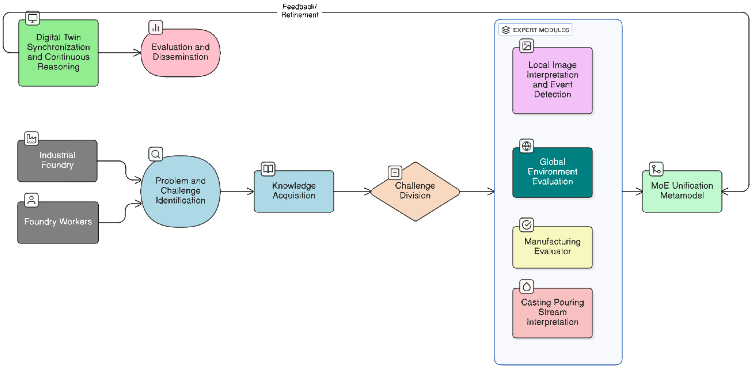
Figure 2.
Schematic top-view of the initial section of a vertical sand-casting foundry, showing the setup used in this study. From right to left, the diagram shows: (i) the mould generation unit (DISA moulding machine), (ii) the pouring area with a press-pour machine and a tile cover to prevent unwanted metal in the next mould, (iii) the sequence of the first 8 moulds (seven already poured and one awaiting or pouring metal), (iv) the camera Field of View (FoV) for video data capture, and (v) several sensors related to the pouring and moulding units.
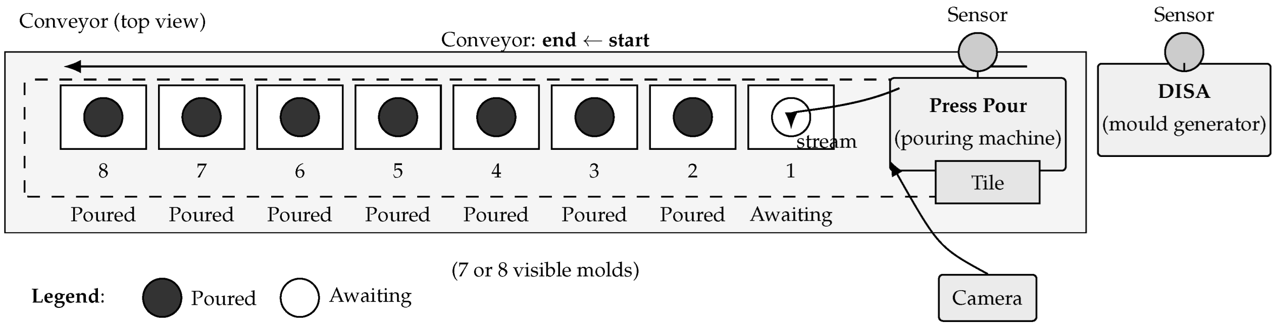
Figure 3.
Actual front-view image of the initial section of the vertical sand-casting foundry corresponding to the schematic shown in Figure 2. The image illustrates the operational setup captured in the experimental videos.
Figure 3.
Actual front-view image of the initial section of the vertical sand-casting foundry corresponding to the schematic shown in Figure 2. The image illustrates the operational setup captured in the experimental videos.
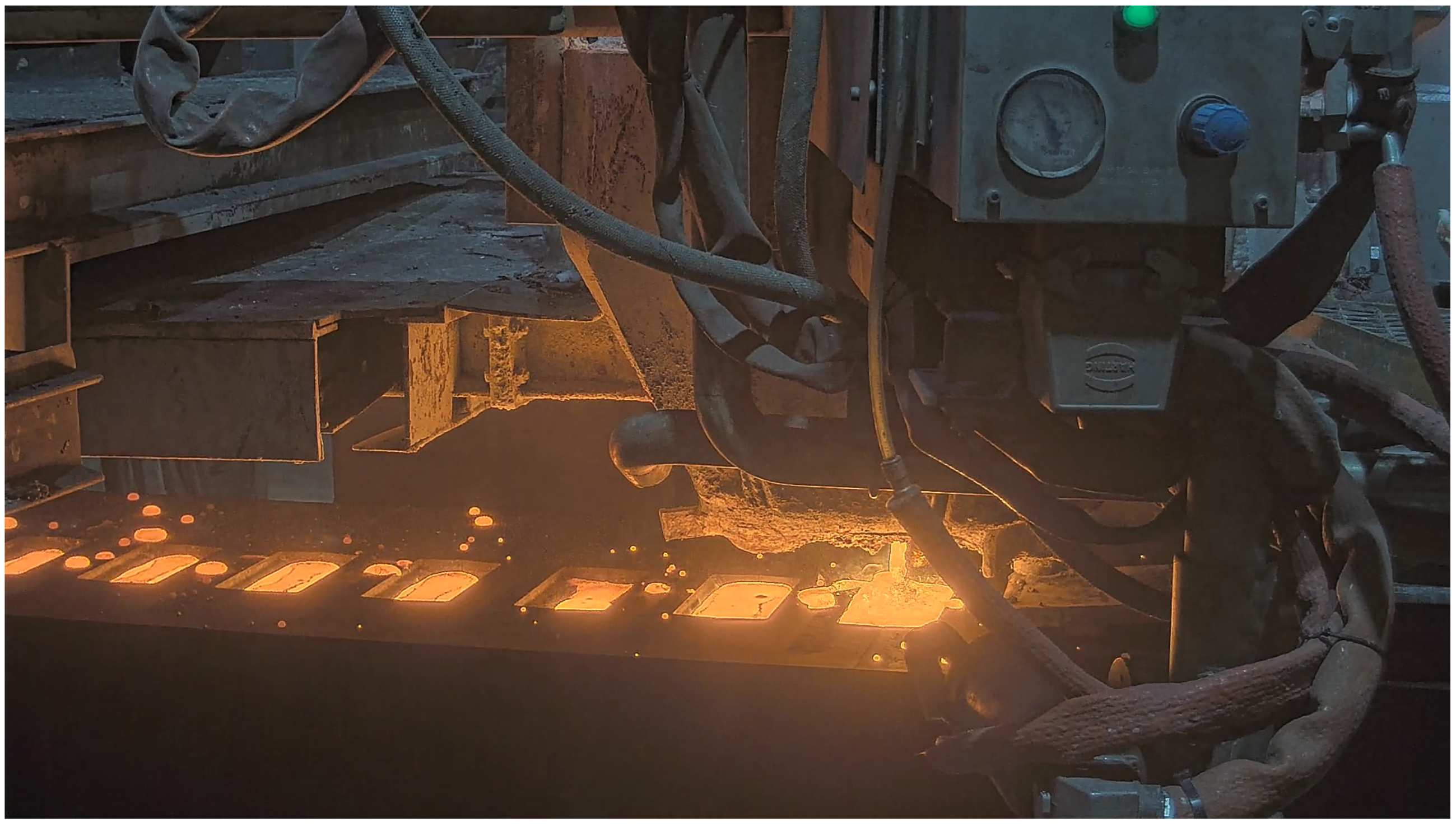
Figure 5.
Representative examples of the four manufacturing context classes considered in this work.
Figure 5.
Representative examples of the four manufacturing context classes considered in this work.
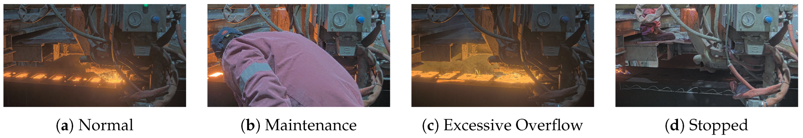
Figure 6.
Region-of-interest (ROI) states detected by the SSIM-based method described in Algorithm 1. The left image shows active conveyor moving with detectable motion in the stream area, while the right image shows the static state after event completion or during pouring.
Figure 6.
Region-of-interest (ROI) states detected by the SSIM-based method described in Algorithm 1. The left image shows active conveyor moving with detectable motion in the stream area, while the right image shows the static state after event completion or during pouring.
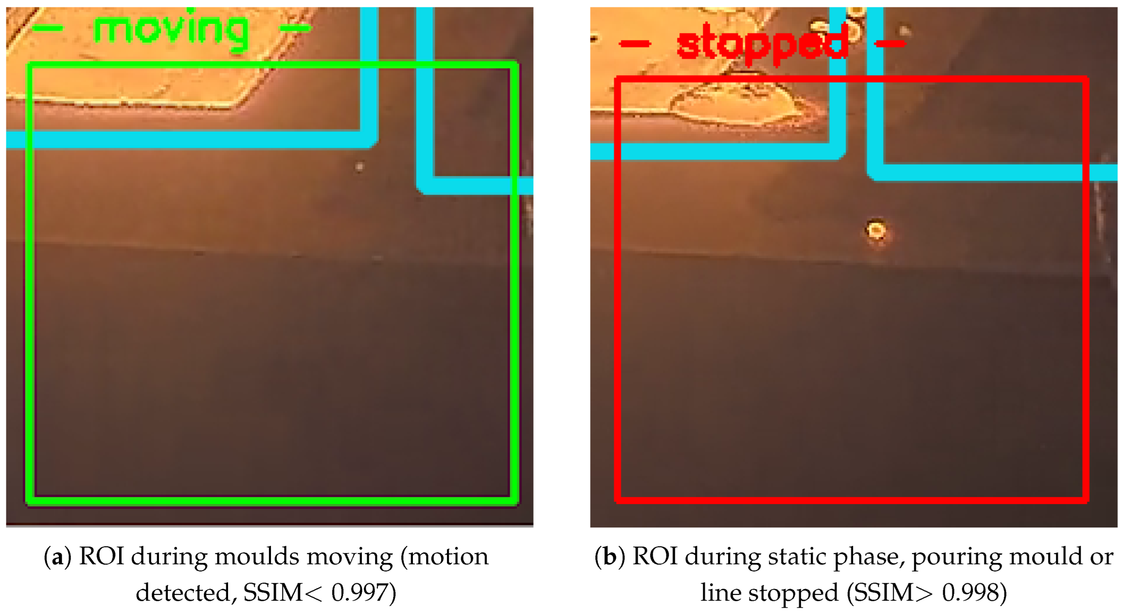
Figure 7.
Conceptual representation of the areas of interest in the pouring zone, highlighting the regions where molten metal enters the mould to form the cast parts. Shown are the pouring stream, the protective tile (covering the next cup), the current and incoming mould cups, and additional moulds travelling on the conveyor. Cups may appear in different filling states (empty, partially filled, fully filled). This schematic summarises the key visual zones later identified by the YOLOv11-based detector [34].
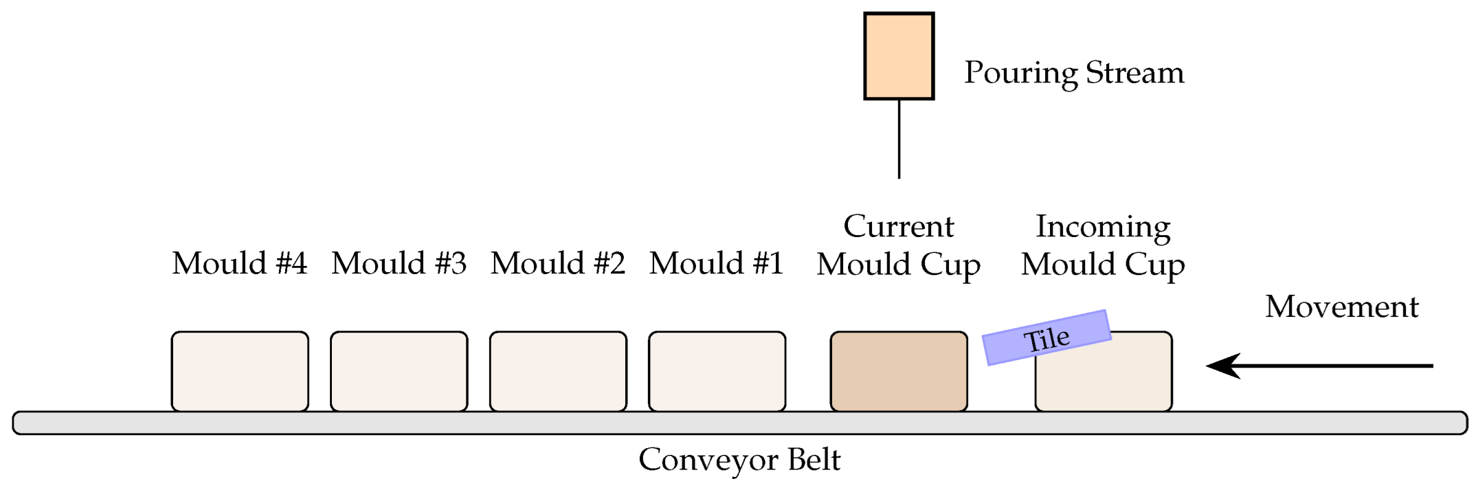
Figure 8.
Example of a frame with overlayed AoI detections.
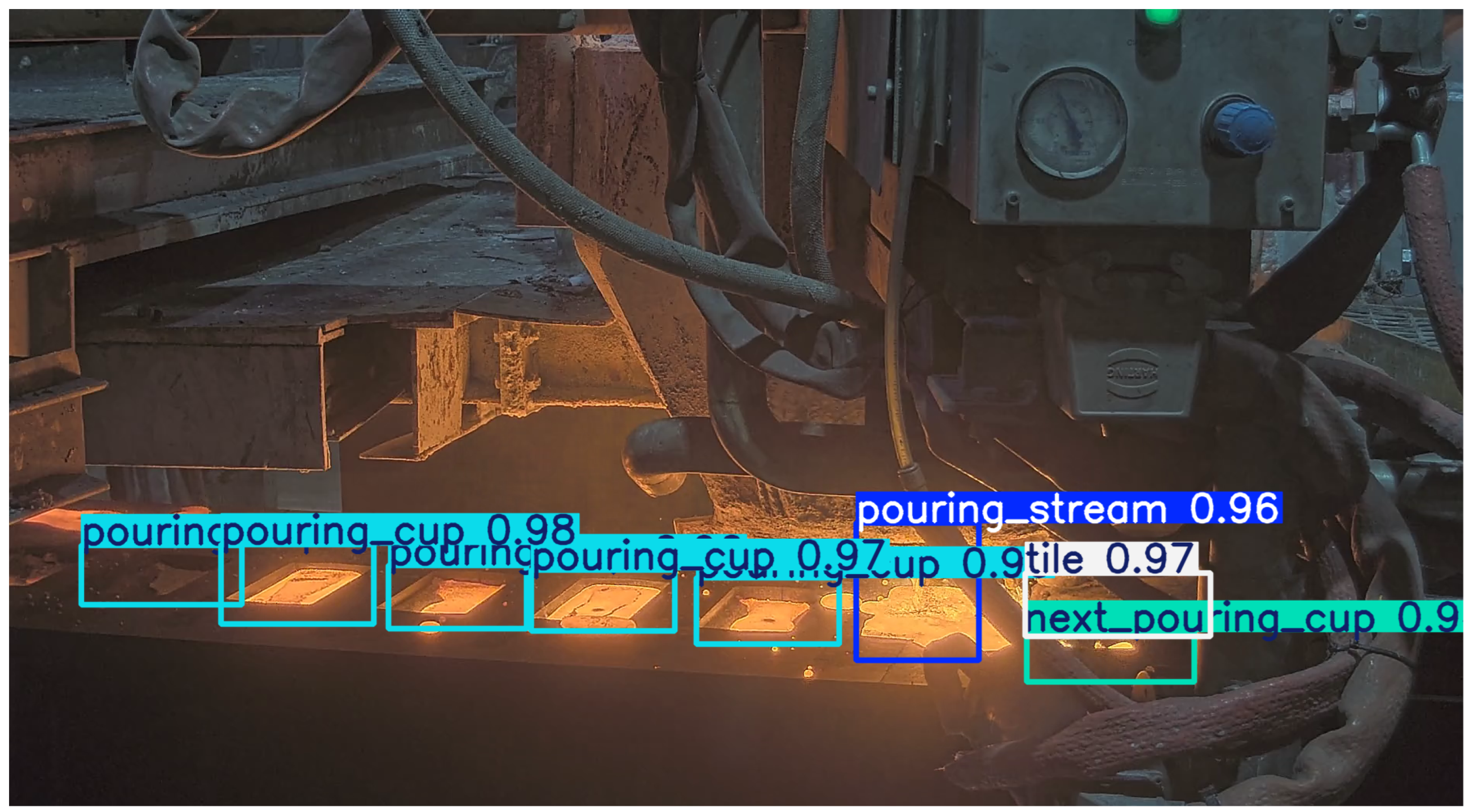
Figure 9.
Representative examples of mould cup classification categories used for AoI classification. Each frame is extracted from production footage and corresponds to the input samples of the YOLOv11 classifier.
Figure 9.
Representative examples of mould cup classification categories used for AoI classification. Each frame is extracted from production footage and corresponds to the input samples of the YOLOv11 classifier.
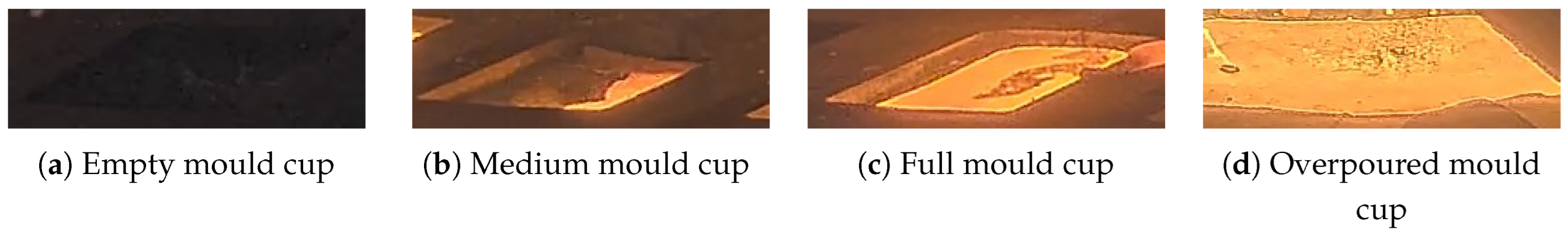
Figure 10.
Examples of incoming mould cup classification. Left image shows normal mould ready for pouring without problems detected. Right image illustrates a warning condition due to residual metal presence.
Figure 10.
Examples of incoming mould cup classification. Left image shows normal mould ready for pouring without problems detected. Right image illustrates a warning condition due to residual metal presence.
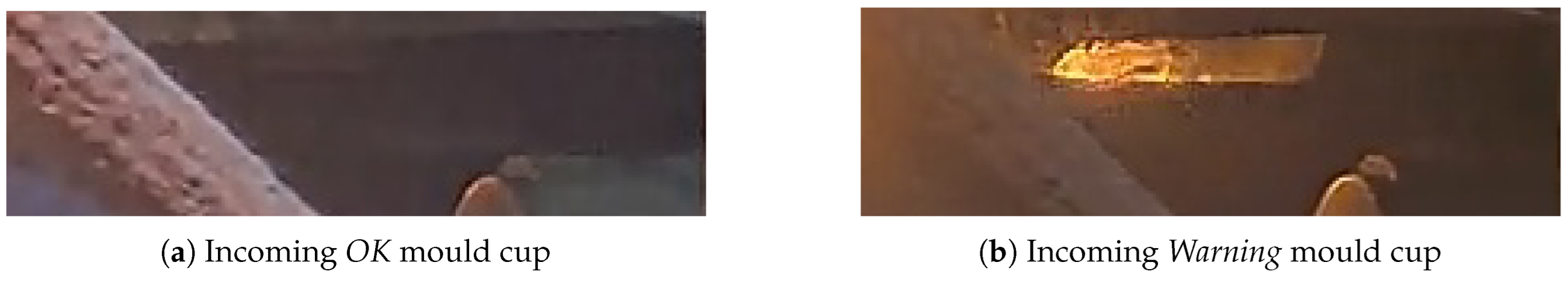
Figure 11.
Compact diagram of the MoE decision system. Specialised experts evaluate temporal limits, stream integrity, mould conditions and operational context; the MoE integrates them into a unified mould event decision.
Figure 11.
Compact diagram of the MoE decision system. Specialised experts evaluate temporal limits, stream integrity, mould conditions and operational context; the MoE integrates them into a unified mould event decision.
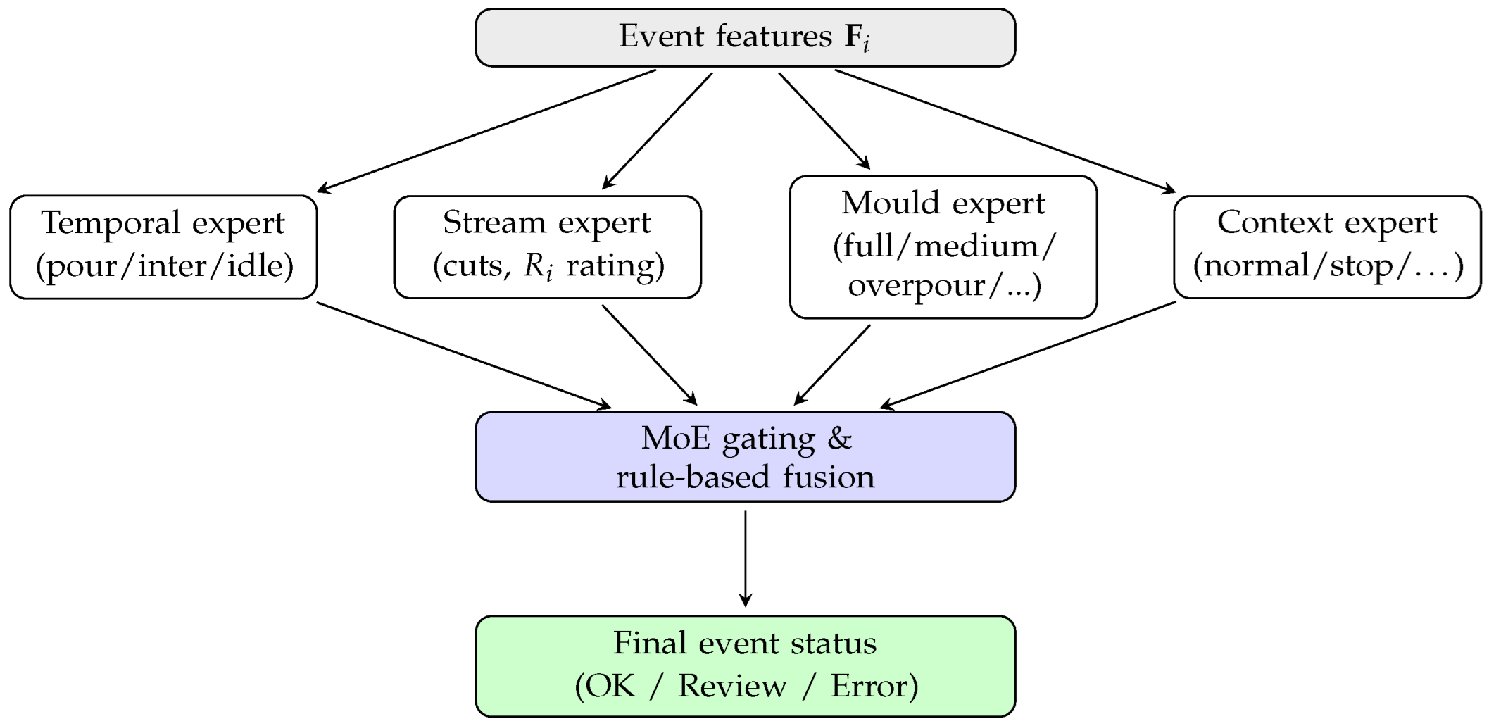
Figure 12.
Training dynamics of the manufacturing context classifier.
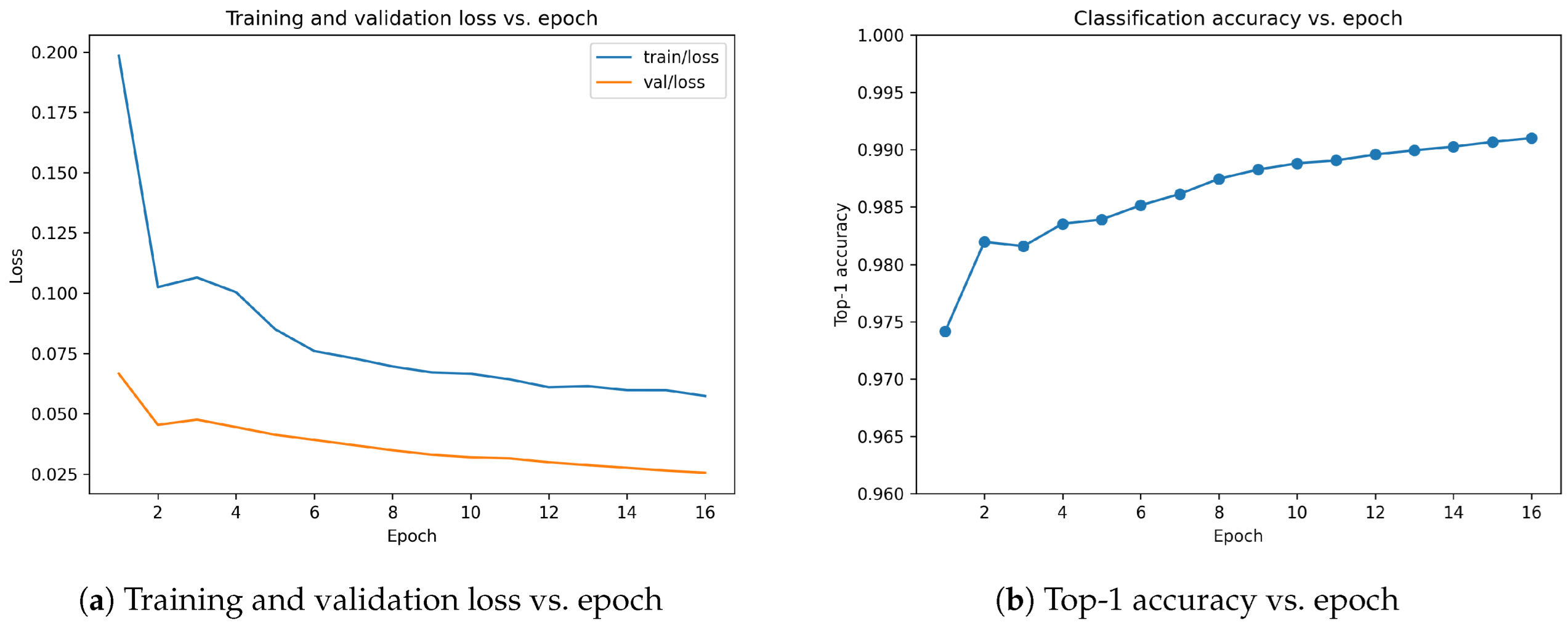
Figure 13.
Precision–recall curves for the four AoI classes. The bold line corresponds to the aggregated performance.
Figure 13.
Precision–recall curves for the four AoI classes. The bold line corresponds to the aggregated performance.
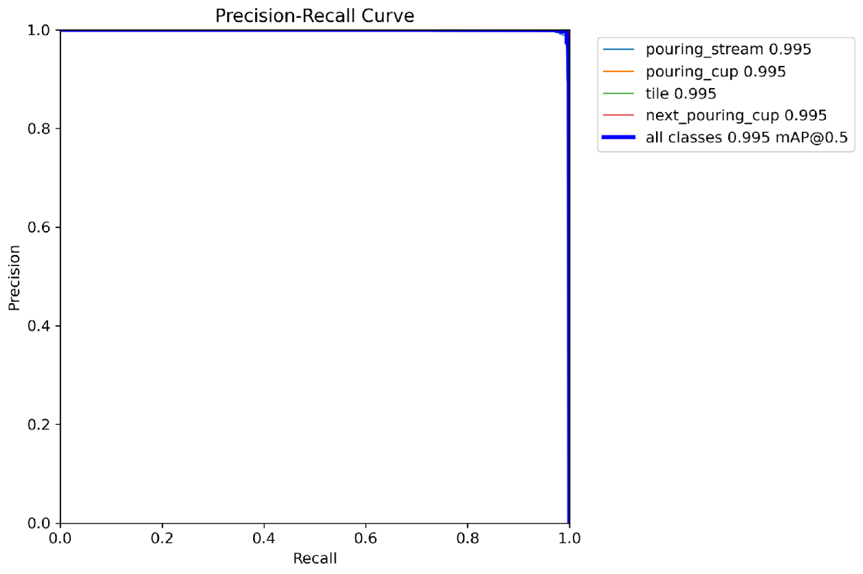
Figure 14.
Accuracy evolution of the mould cup filling state classifier.
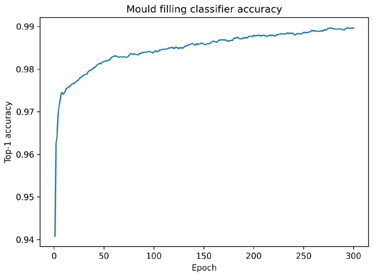
Figure 15.
Training behaviour of the incoming mould cup classifier. The accuracy curve shows the evolution of top-1 accuracy on the validation set, which stabilises above 0.98.
Figure 15.
Training behaviour of the incoming mould cup classifier. The accuracy curve shows the evolution of top-1 accuracy on the validation set, which stabilises above 0.98.
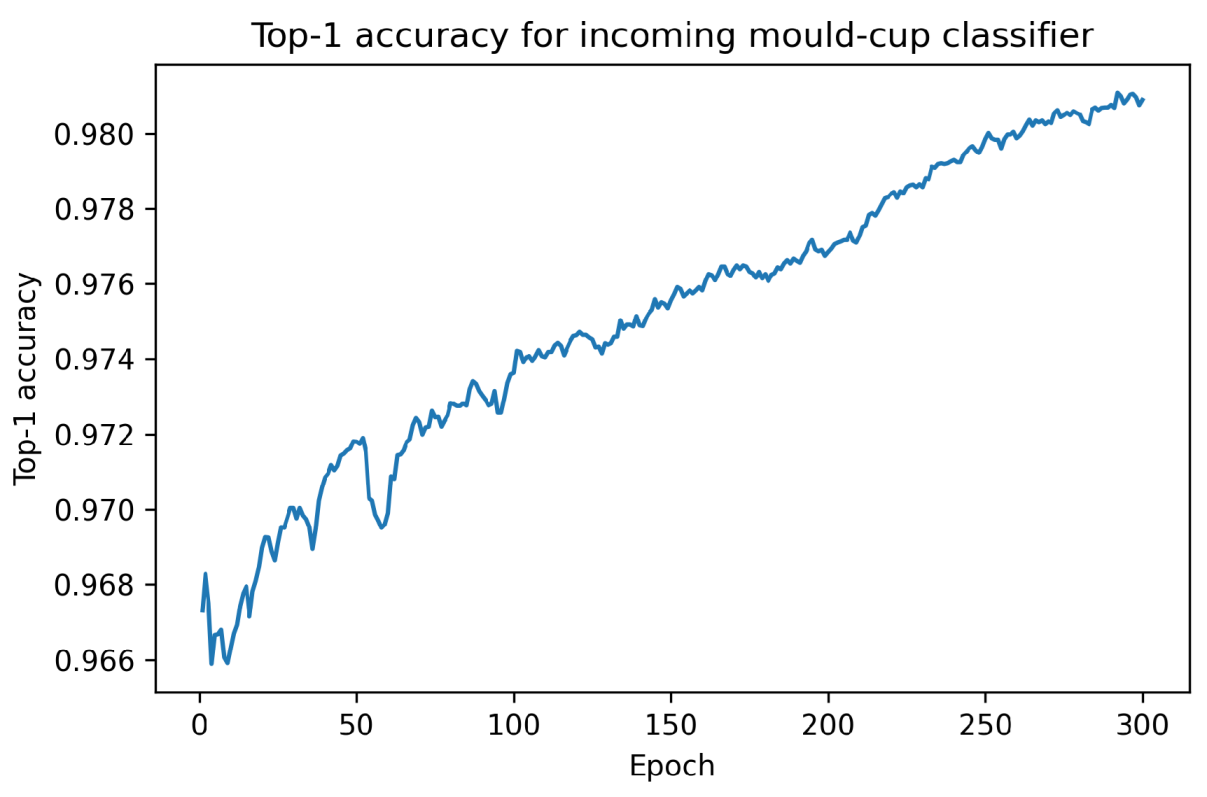
Figure 18.
TSNE visualization of the clustering results for K-Means.
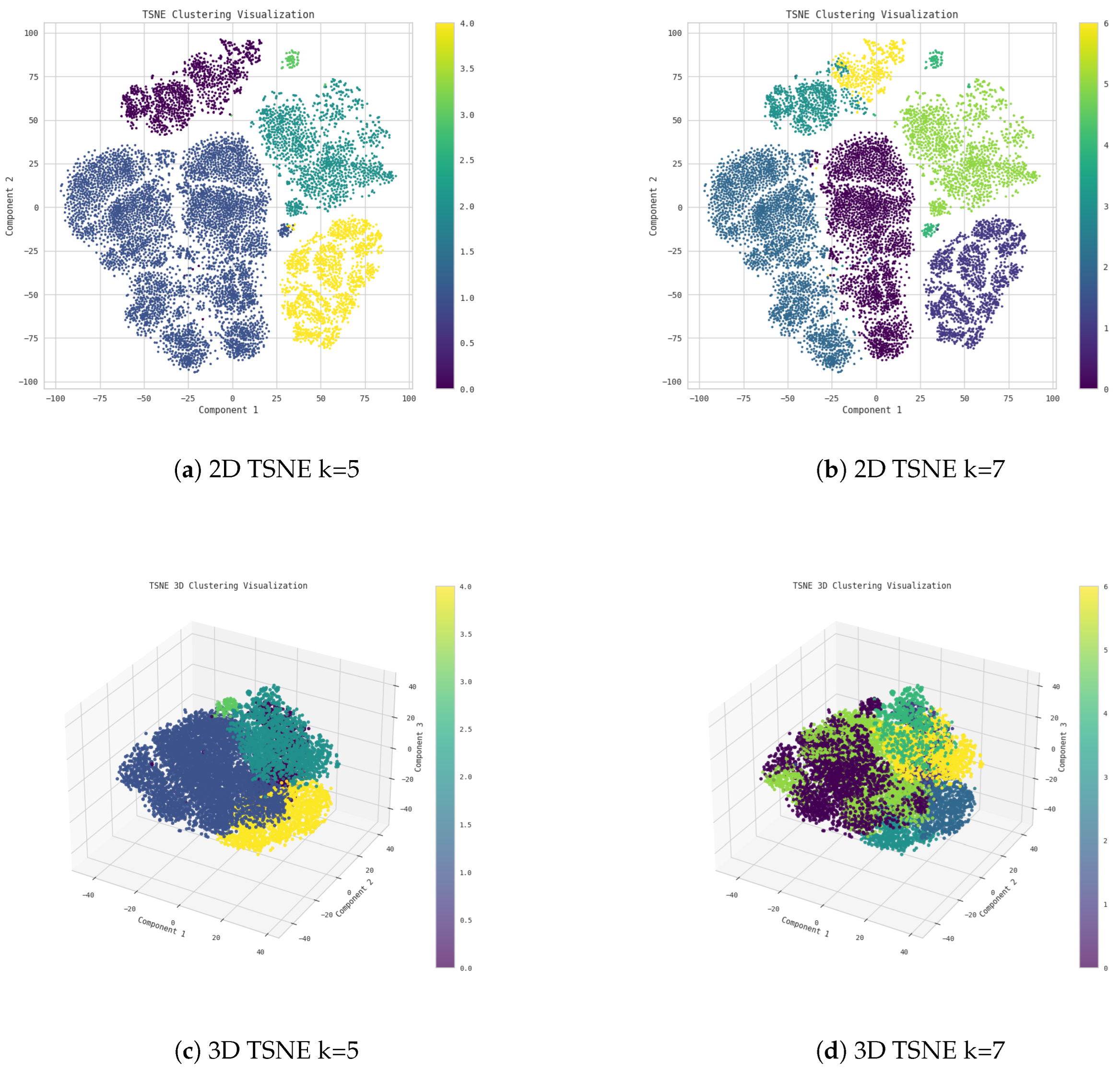
Figure 19.
Outliers and small clusters found by DBSCAN for vision only features across various parameters combination for and min_samples. a) Number of samples left as outliers; b) Number of overly-specific small clusters.
Figure 19.
Outliers and small clusters found by DBSCAN for vision only features across various parameters combination for and min_samples. a) Number of samples left as outliers; b) Number of overly-specific small clusters.
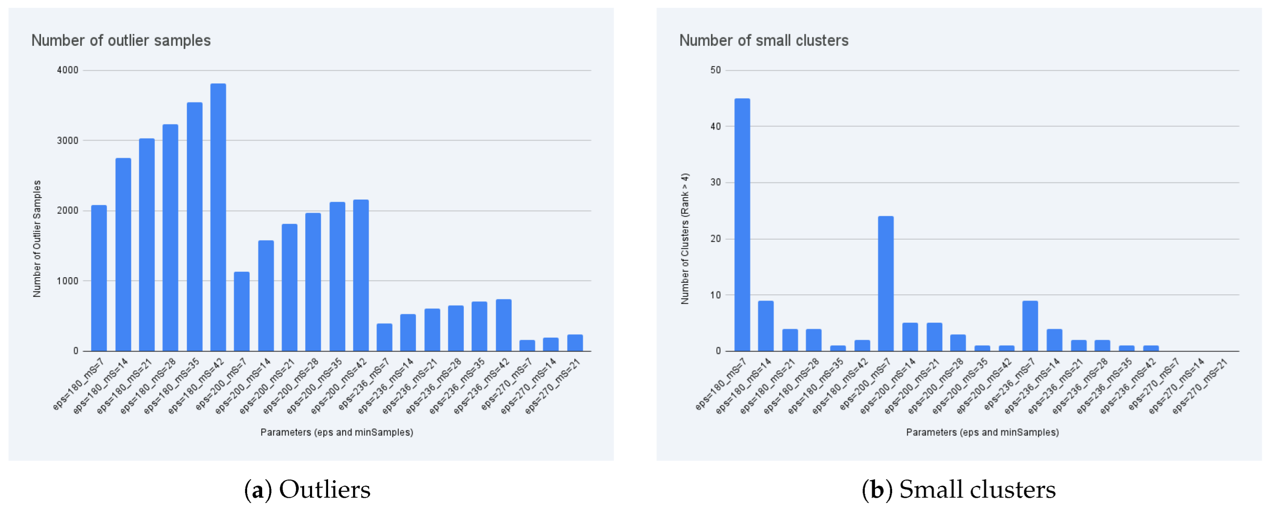
Figure 21.
Examples of expected anomalies found with DBSCAN.
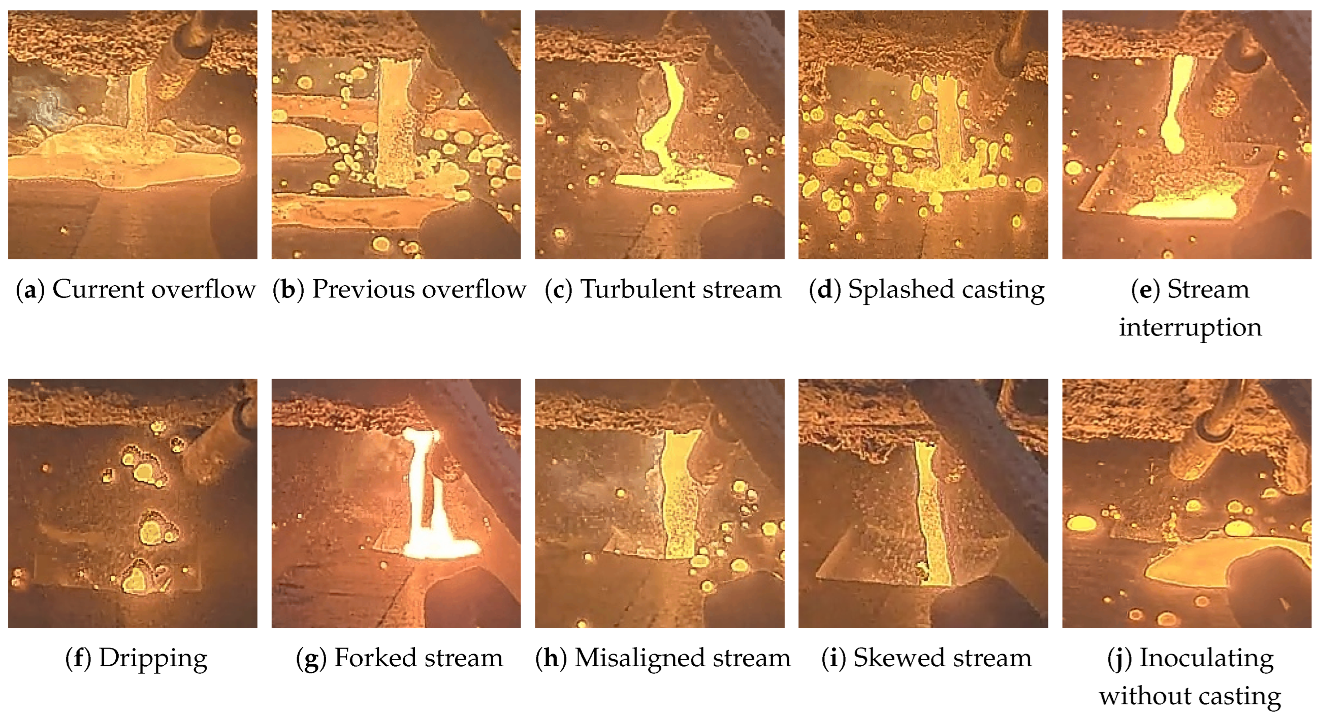
Figure 22.
Examples of anomalies caused by a problem/limitation in sampling found with DBSCAN.
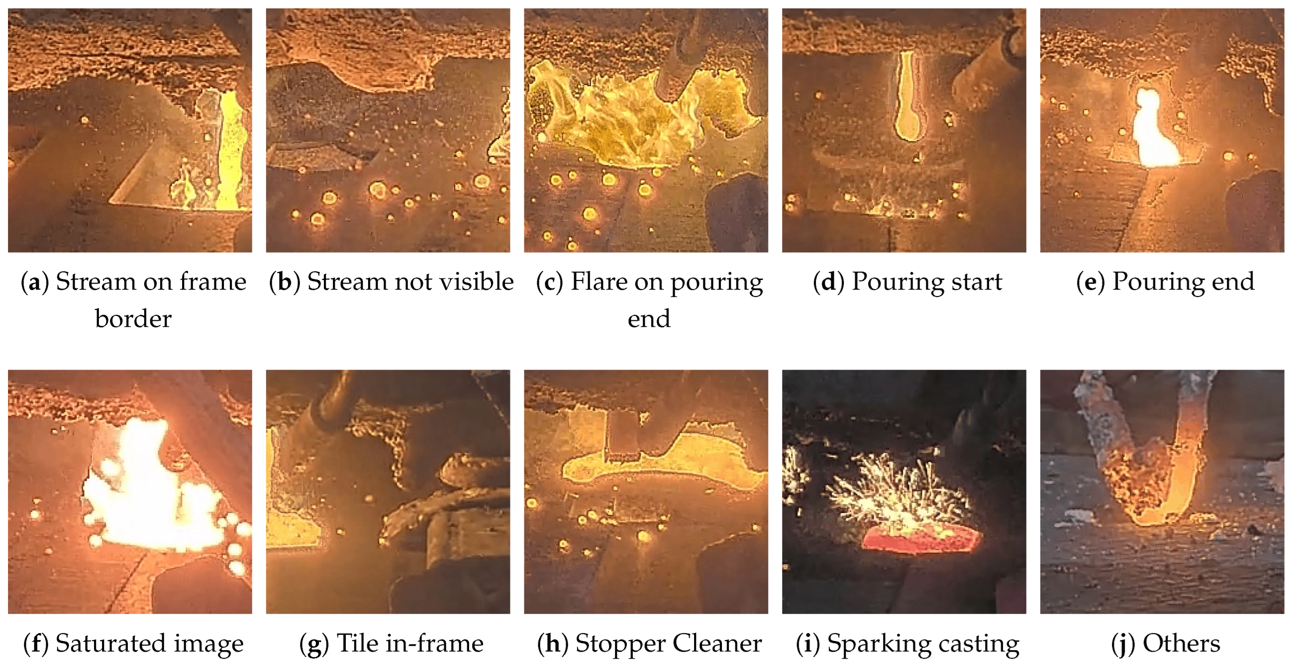
Figure 25.
Agreement results in number of pouring events classified as anomalies using for the pouring events detailed in Table 2
Figure 25.
Agreement results in number of pouring events classified as anomalies using for the pouring events detailed in Table 2
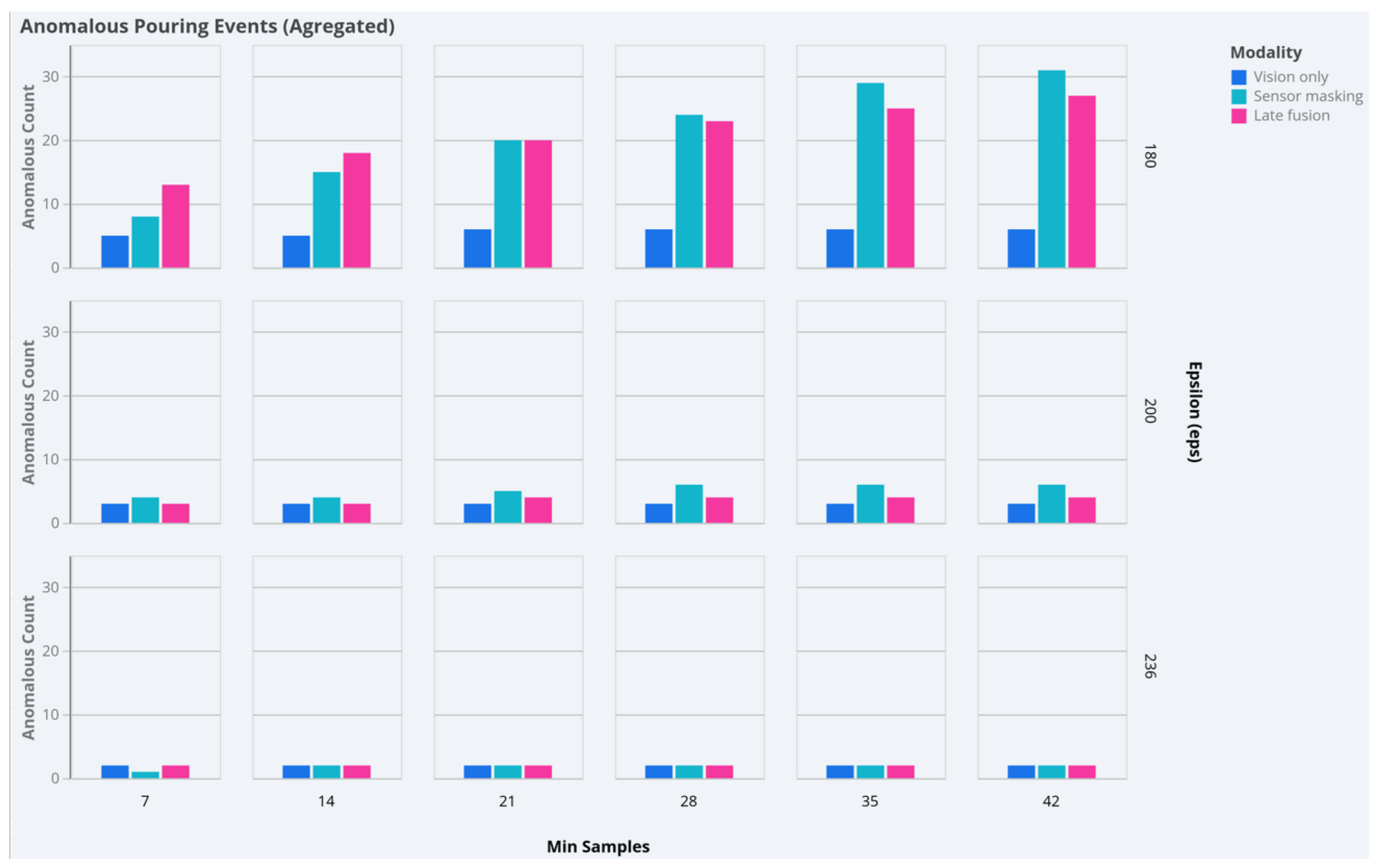
Table 1.
Overview of the different subsystems monitored in the experimental foundry, obtained by grouping the 155 recorded process signals into functional areas. This abstraction highlights the main data sources that feed the multimodal model, while hiding the identifiers due to confidentiality issues.
| Foundry subsystem | # Signals | Representative variables / description |
|---|---|---|
| Moulding (DISA) | ∼35 | Sand compression pressure, compaction density, mould ejector and closure sensors. |
| Pouring (Press-Pour) | ∼40 | Molten metal temperature, stopper valve position, pouring enable signal, metal level sensors. |
| Conveyor and cooling line | ∼25 | Conveyor speed, mould index counter, cooling temperature and airflow. |
| Auxiliary and safety systems | ∼30 | Line active flag, air pressure, emergency stop, interlocks, plant readiness indicators, operation enable flags. |
| Quality and traceability | ∼25 | Mould rejection flag, reference change detection, operator action marker. |
Table 2.
Quantitative evaluation of the pouring event detector over 1 hour of production video.
| Real moulds | 562 |
| Detected moulds | 539 |
| Absolute error | 23 |
| Accuracy | 95.91% |
| Detected/real ratio | 0.9589 |
| Real rate | 9.37 moulds/min |
| Detected rate | 8.98 moulds/min |
Table 3.
Normalised confusion matrix of the YOLOv11 AoI detector. Rows indicate predicted classes and columns indicate ground-truth labels.
Table 3.
Normalised confusion matrix of the YOLOv11 AoI detector. Rows indicate predicted classes and columns indicate ground-truth labels.
| Real | pouring_stream | pouring_cup | tile | next_pouring_cup | background | |
|---|---|---|---|---|---|---|
| Predicted | ||||||
| pouring_stream | 0.99 | 0 | 0 | 0 | 0.23 | |
| pouring_cup | 0 | 1.00 | 0 | 0 | 0.73 | |
| tile | 0 | 0 | 1.00 | 0 | 0.02 | |
| next_pouring_cup | 0 | 0 | 0 | 1.00 | 0.02 | |
| background | 0 | 0 | 0 | 0 | 0 | |
Table 4.
Descriptive statistics extracted from the parsed POURING_EVENT logs (539 events). Percentiles highlight the typical operating band and the presence of rare long-tail delays.
Table 4.
Descriptive statistics extracted from the parsed POURING_EVENT logs (539 events). Percentiles highlight the typical operating band and the presence of rare long-tail delays.
| Variable | Mean | Std | Median | P05 | P95 | Min | Max |
|---|---|---|---|---|---|---|---|
| Pour duration [s] | 4.90 | 0.29 | 4.90 | 4.30 | 5.45 | 0.00 | 8.70 |
| Inter-pour time [s] | 3.49 | 0.84 | 3.50 | 3.25 | 3.75 | 0.00 | 21.70 |
| Idle time [s] | 1.78 | 0.26 | 1.80 | 1.40 | 2.25 | 0.00 | 3.80 |
| Cycle time [s] | 8.39 | 0.89 | 8.40 | 8.00 | 8.75 | 0.00 | 23.60 |
Table 5.
Summary of MoE decisions obtained from the analysed pouring events (a one hour video with 539 detected cycles).
Table 5.
Summary of MoE decisions obtained from the analysed pouring events (a one hour video with 539 detected cycles).
| MoE decision | Number of events | Percentage (%) |
|---|---|---|
| OK | 492 | 91.3 |
| Review | 32 | 5.9 |
| Not_OK | 15 | 2.8 |
| Total | 539 | 100.0 |
Table 6.
Dominant contributing factors associated with each MoE decision outcome.
| MoE decision | Main contributing indicators |
|---|---|
| OK | Stable pouring stream, zero or negligible interruptions (), filling state classified as full or medium, pouring duration within control limits, and absence of abnormal operational context. |
| Review | Short or isolated stream interruptions (), mild turbulence episodes, overpouring conditions treated as warning states, borderline pouring duration or inter pouring time, or partial overlap with non-regular context segments (e.g. brief maintenance occlusions). |
| Not_OK | Recurrent stream cuts, persistent violations of temporal constraints, incorrect filling states (empty), severe material loss, or clear presence of safety alerts on incoming mould cups. Overpouring alone does not trigger a Not_OK decision unless combined with instability, material loss, or safety risks. |
Disclaimer/Publisher’s Note: The statements, opinions and data contained in all publications are solely those of the individual author(s) and contributor(s) and not of MDPI and/or the editor(s). MDPI and/or the editor(s) disclaim responsibility for any injury to people or property resulting from any ideas, methods, instructions or products referred to in the content. |
© 2026 by the authors. Licensee MDPI, Basel, Switzerland. This article is an open access article distributed under the terms and conditions of the Creative Commons Attribution (CC BY) license (http://creativecommons.org/licenses/by/4.0/).
Copyright: This open access article is published under a Creative Commons CC BY 4.0 license, which permit the free download, distribution, and reuse, provided that the author and preprint are cited in any reuse.


