Submitted:
23 February 2026
Posted:
25 February 2026
You are already at the latest version
Abstract
The simulation of synthetic aperture radar (SAR) echo signals usually relies on complex hardware equipment and a large amount of scene data, which results in high costs and low efficiency. In order to simulate SAR echo signals of ship targets in the sea quickly and accurately in complex environments at a lower cost, this paper proposes a SAR echo simulation method based on model segmentation and electromagnetic scattering characteristic simulation. This method first implements the simulation of sea models under different sea conditions based on PM wave spectrum model and Monte Carlo method, and segments them according to the requirements of simulation resolution. Then, it uses Python API in Blender to segment the ship model automatically and optimize the visible surface elements and mesh for each sub-model. Next, it uses Lua API in Feko to simulate the electromagnetic scattering characteristics of each sub-model of the sea surface and the ship target automatically, and obtains the required radar cross section (RCS) data of ship target in the sea after processing. Finally, SAR echo simulation is realized through time-domain algorithm. To further verify the simulation result, the chirp scaling (CS) algorithm is used for imaging processing. The results show that this method can realize SAR echo simulation of various ship targets under different sea conditions in a quick, accurate and cost-effective manner without the need for any hardware equipment.
Keywords:
synthetic aperture radar (SAR)
; radar echo simulation
; model segmentation
; electromagnetic scattering simulation
; radar cross section (RCS)
1. Introduction
The ocean serves as a connecting link among countries around the world. With the increasing frequency of marine resource exploitation and global maritime activities, the monitoring of ship targets in the sea has become a key technical requirement for safeguarding maritime rights and maintaining maritime security [1]. Synthetic aperture radar (SAR) is a high-resolution active remote sensing technology. Due to its immunity to factors such as light and climate, it can operate all day long through the year, and can identify various ship targets in complex sea environments accurately [2,3]. Therefore, it plays a significant role in the monitoring of surface ship targets.
Obtaining real SAR echo signals of ship targets in the marine environment is not only costly and inefficient, but also subject to various limitations such as weather, equipment, and activity patterns of the targets. Therefore, establishing a high-precision simulation system to simulate SAR echo data in actual scenarios is of great significance. By simulating SAR echo signals, various complex marine scenarios can be precisely simulated, including the characteristics of sea clutter under different sea conditions, the movement patterns of different ship targets, and different SAR imaging mechanisms [4,5,6]. This provides a virtual testing environment for the design and optimization of SAR systems, helping to analyze the system performance deeply and reducing the cost and risks of actual development.
The simulation technology for SAR echo signals of ship targets in the sea can be traced back to 1970s. With the rapid development of SAR technology, researchers began to focus on the spatial distribution characteristics of echo signals and attempted to generate original data of SAR system through numerical simulation. In 1978, V.H. Kaupp and J.C. Holtzman developed a Ku-band radar simulation system, which has the ability to simulate multi-terrain echo signals. However, due to the insufficient completeness of backscatter coefficient database, the application of this system was severely limited for a long time [7]. In 1995, Soumekh proposed a SAR echo simulation method based on ray tracing, using the geometric characteristics of target and the electromagnetic scattering model to establish an echo simulation framework for complex scenarios, laying the foundation for subsequent simulation research on ship targets [8]. In 2002, Brown developed a SAR echo simulation algorithm based on physical optics and electromagnetic scattering theory. This method, for the first time, combined sea surface roughness and geometric characteristics of ships, and was able to simulate scattering characteristics of ship targets under different sea conditions accurately, significantly enhancing the realism and accuracy of echo simulation [9]. In 2005, Wang proposed a two-dimensional sea clutter modeling method based on Fourier transformation, which for the first time generated a realistic dynamic sea model by combining actual sea condition observation data, and simulated scattering characteristics of ship targets, providing a theoretical basis for SAR simulation technology in complex marine environments [10]. In 2007, Danisi, A. proposed a SAR echo simulation method for specific marine scenarios. This method focused on complex situation where the ocean surface is covered by randomly shaped oil pollution, aiming to simulate and obtain SAR echo data in this special environment [11]. In 2021, Jiang proposed a wideband radar echo simulation method for targets on dynamic sea surfaces. The method adopts a frequency-domain framework combined with a hybrid scattering model to calculate target electromagnetic responses, and uses IFFT to generate SAR echoes. The results demonstrate that dynamic sea motion and multiple scattering affect imaging quality significantly, improving the physical realism of wideband SAR ship echo simulation [12]. In 2024, Yao proposed a SAR echo simulation method for sea surface scenes combined with electromagnetic scattering characteristics. This method integrates dynamic sea surface modeling with electromagnetic scattering mechanisms and establishes a unified simulation framework that considers both time-varying ocean wave motion and target–sea composite scattering effects. By incorporating physical optics and related scattering models into SAR echo generation process, the approach improves the physical consistency and realism of simulated SAR images under complex marine environments, providing a more accurate basis for ship detection and scene interpretation in ocean scenarios [9].
The acquisition of complex environmental and target electromagnetic scattering characteristics is a key issue in SAR echo simulation process. Therefore, scholars have conducted a large number of studies on this. Currently, the mainstream methods for calculating electromagnetic scattering characteristics are mainly divided into two categories: those based on physical models and those based on empirical models [12].
The method based on physical models starts from actual physical characteristics of the target and describes the interaction between target and radar waves precisely, thereby simulating and calculating the target’s scattering ability to radar waves accurately [13]. In 2002, Mallorgui used a high-frequency approximation model and combined with the electromagnetic scattering characteristics of ship targets to generate airborne SAR fully polarized simulation echo data for ship targets [14]. In 2003, G. Franceschetti used Kirchhoff method and combined with multiple scattering effect of electromagnetic waves, simulated the electromagnetic scattering characteristics of urban structures effectively and obtained corresponding SAR echo data through simulation [15]. In 2022, Rao proposed a high-frequency electromagnetic scattering simulation method for anisotropic plasma-coated electrically large and complex targets, combining the Physical Optics Method (PO) with spectral domain expansion to compute the scattering characteristics and analyze the propagation mechanisms within plasma layers efficiently [16]. In 2024, Hu presented a two-dimensional electromagnetic scattering analysis method based on the Boundary Element Method with NURBS surface representation, enabling high-precision simulations without dense volumetric meshing and providing shape sensitivity analysis for target optimization [17]. The method based on physical models involves complex mathematical operations and a large number of solving processes of parameters, resulting in low computational efficiency. Therefore, it is usually used for precise calculations of relatively small targets, such as buildings and aircraft [18].
The method based on empirical models takes a statistical approach. By analyzing a large amount of experimental data and measurement results, it discovers potential relationships between electromagnetic scattering characteristics and various parameters, and establishes corresponding empirical equations [19]. Therefore, it can achieve efficient simulation of large-scale natural scenes such as oceans, lands, and forests while maintaining a certain level of accuracy. In 1997, Robert L. developed a Monte Carlo simulation method for electromagnetic scattering from two-dimensional random rough surfaces, combining statistical surface realizations with the Fast Multipole Method (FMM) to efficiently compute ensemble-averaged bistatic scattering coefficients and analyze backscattering enhancement effects [20]. In 2001, M. El-Shenawee applied a Monte Carlo-based electromagnetic scattering simulation to random rough surfaces with buried objects, integrating fast multipole techniques to evaluate the statistical characteristics (mean and variance) of scattered fields and to study the influence of surface roughness on subsurface target detection [21]. In the same year, K. Tang proposed a statistical model for electromagnetic wave scattering from random rough surfaces, in which surface height distributions and correlation functions were used to characterize roughness, and the scattered fields were predicted based on statistical geometric parameters under geometric optics assumptions [22]. In 2010, Monsivais Huertero, based on the statistical method, considered the specific positions of grass leaf, stem, and stalk on scattering characteristics in the study of electromagnetic scattering characteristics of grassland scenes and established a coherent scattering model for the Saharan grassland [23]. In 2016, Huating Huang and Kim further improved the related scattering model of soybeans by introducing conditional probability density functions and combining the related scattering among particles [24].
In order to improve the simulation efficiency while ensuring accuracy and reduce costs, this paper has referred to and improved various methods, combined with multiple software such as Blender and Feko, and proposed a SAR echo simulation method for ship targets in the sea based on model segmentation and electromagnetic scattering characteristics simulation. The subsequent content arrangement of this paper is as follows: The second part consists of four sections, which respectively explain the research contents and methods such as sea model simulation and segmentation, ship target model segmentation, electromagnetic scattering characteristics simulation of sea surface and ship targets, and SAR echo simulation; The third part corresponds to the second part, presenting results of each study and conducting analysis and verification; The fourth part conducts a comprehensive analysis and discussion on application value, shortcomings, and subsequent improvement directions of the research content of this paper.
2. Materials and Methods
2.1. Simulation and Segmentation of Sea Model
The simulation of sea model is based on the PM wave spectrum model and is implemented using the Monte Carlo method.
Wave spectrum refers to the distribution of wave energy on sea surface in terms of frequency and direction. It is obtained through Fourier transform of the autocorrelation function of sea surface height variations and reveals the second-order statistical characteristics of waves and the distribution laws of wave energy in different wavelengths and directions. By establishing an actual sea model based on wave spectrum, the wave fluctuation characteristics under various sea conditions can be described, which helps to improve accuracy, prediction ability and practical application of the sea surface electromagnetic scattering model, and reveal the influence of different marine environments on electromagnetic wave scattering [25,26]. The common used wave spectrum includes the PM spectrum, the JONSWAP spectrum, the Elfouhaily spectrum, etc.
The PM wave spectrum is one of the most classic and fundamental empirical wave spectrum models. It was derived by Pierson and Moskowitz based on the analysis of a large amount of measured data from the North Atlantic. Its core assumption is that the sea surface is in a fully developed state, that is, the wind speed is constant, the wind direction is constant, the wind blowing time is long enough, and the wind blowing distance is infinite. At this time, wave energy will only be determined by wind speed and reach statistical equilibrium [27,28]. The PM wave spectrum can be expressed as follows:
where and are dimensionless empirical constants, is the gravitational acceleration, is wave number and is wind speed at a height of 19.5 meters above sea level. Its relationship with , wind speed at a height of 10 meters above sea level is: .
Internationally, the sea states codes based on Douglas sea scale is commonly used to describe the level of ocean waves. It uses wind speed and wave height to describe specific changes on the sea surface. The corresponding relationship is shown in Table 1 [29].
The Monte Carlo method conducts inversion simulation based on wave spectrum model, thereby obtaining actual wave fluctuations. It is the most commonly used two-dimensional linear sea surface modeling method. This method regards waves as a superposition of a series of harmonics with different wavelengths, periods, and initial phases. Firstly, it converts the white noise to frequency domain through Fourier transformation. Then, it uses wave spectrum to filter the result. Finally, it obtains the expression of filtered rough sea surface height fluctuations through inverse Fourier transformation [30,31]:
where , , , and respectively represent the total length of the sea surface in and directions. is a complex Gaussian random sequence, denotes taking complex conjugate, represents two-dimensional sea spectrum. To ensure that the sea surface height is a real number, the Hermitian form of equation should satisfy following condition:
Finally, through IFFT, it obtains that:
Throughout the entire process, FFT and IFFT are required. Therefore, the spatial geometric length of the sea surface needs to be discretized, and at the same time, the Nyquist theorem must be satisfied:
where represents the sampling frequency in direction, represents the sampling interval of . Similarly, the sampling in direction also needs to comply with the Nyquist theorem. and respectively represent cutoff wavenumber and minimum wavenumber, and their values determine bandwidth of the band to be extracted on the wave spectrum. Due to different energy intervals of wave spectrum corresponding to different wind speeds, it is necessary to ensure that the energy distribution range of the wave spectrum under current wind speed is as much as possible included within the wave number range [32].
In order to facilitate the subsequent simulation of electromagnetic scattering characteristics, the complete sea model needs to be divided into multiple sub-blocks, and each sub-block should be triangulated. Then, it should be saved as a STL format file. STL format is the most common file format in 3D printing field, which is used to record triangular face element data of the model surface. The principle of converting ordinary matrix data into STL format is shown in Figure 1.
The STL format file stores two matrices, P and T. Matrix P converts the data in original two-dimensional matrix H into a one-dimensional matrix, while matrix T is composed of multiple three-dimensional vectors. Each vector records the sequence of three vertex data of a certain triangular face element in matrix P. In this paper, a local data matrix H is extracted from the complete sea model and converted into matrix P each time. Then, an autonomous design combination algorithm is used to generate matrix T, so that every four (2*2) adjacent sampling points in matrix H form a square that is divided into two triangular face elements in “upper right - lower left” manner. Finally, it is exported in STL format to achieve the segmentation of entire sea model.
2.2. Ship Target Model Segmentation
The segmentation of ship target model is achieved through Blender. Blender is a powerful and lightweight 3D graphics and image software that offers a wide range of functions such as 3D modeling, materials and textures, animation system, rendering engine and visual effects. It also has a complete Python API that enables quick execution of various operations within the software, making it highly suitable for large-scale repetitive model segmentation tasks [33].
The main steps for model segmentation in Blender are shown in Figure 2.
- Import model file and create a copy to avoid operating on the initial model directly, as shown in Figure 2a;
- Set segmentation units and construct a rectangular prism cutter based on the requirements of simulation resolution, as shown in Figure 2b;
- Create a Boolean modifier, adjust the solver parameters, perform a Boolean intersection operation on the cutter and the model copy, as shown in Figure 2c;
- Utilize ray detection method to optimize the segmentation results. Emit rays from the location of SAR towards the model, remove completely invisible elements and clean up isolated edges and vertices, as shown in Figure 2d;
- Export the segmentation results in STL format and delete the temporary objects.
By using Python script programs, the above operations can be carried out automatically. Firstly, construct a temporary rectangular cutter. Then, determine the boundary values around entire model manually and build a segmentation grid according to the requirements of simulation resolution. Next, realize the above model segmentation function by writing a script program and adjusting construction position of the cutter through grid coordinates continuously. Finally, the automatic segmentation function of entire model is achieved.
2.3. Simulation of Electromagnetic Scattering Characteristics of Sea Surface and Ship Targets
The electromagnetic scattering characteristics simulation of sea surface and ship targets is achieved through Feko. Feko is a powerful three-dimensional full-wave electromagnetic field simulation software, renowned for its hybrid solution technology and ability to handle problems involving large-scale and complex structures. It also includes a comprehensive Lua API, enabling the automation of electromagnetic scattering characteristic simulation tasks for a large number of models through script programming.
Feko possesses a wide range of solution methods which are applicable to various different simulation scenarios, such as the Method of Moments (MOM), the Finite Element Method (FEM), the Multi-Layer Fast Multipole Method (MLFMM), as well as the PO Method, the Geometrical Optics Method (GO), and the Large Element Physical Optics Method (LEPO), which are adapted to high-frequency conditions.
The PO method is based on integral equations and is grounded on surface currents. It assumes that each point on the scattering body is largely independent of other points, and the resulting effects can be disregarded. By decomposing the target into many triangular sub-element surfaces and solving the scattering fields of each sub-element independently based on the integral of incident field, sum of all the element solutions is thus obtained. Since the summation of scattering fields of the triangular sub-element surfaces is achieved by converting area integral into an integral-free calculation, the computational load is reduced and the calculation speed is improved, making it very convenient to solve scattering fields of large-scale electrical objects [34,35]. Figure 3 shows the schematic diagram of electromagnetic scattering model of the PO method, where and are incident fields, and are scattering fields, is unit normal vector of the target, and and are surface currents and surface magnetic flux densities of the target.
From Stratonovich-Zhilin Integral Equation of Electromagnetic Field, it can obtain that:
where represents the gradient of free-space Green’s function,
where represents the distance from the source point to the field point. The calculations of target surface current and surface magnetic flux density are shown as follows:
where and represent the density of target surface charges and surface magnetic charges. By rearranging the above equation, it can obtain that:
In the process of grid division using the PO method, grid edge length is limited by wavelength. When the incident frequency is high and the target is large, the number of grids to be divided is extremely large, and the requirements for memory and time in the solution process are still relatively high. The LEPO method improves it by correcting the phase of basis function and using multiple wavelengths to divide the target. This reduces the number of divided grids significantly, thereby reducing memory and time required for the calculation, which is conducive to the simulation of electromagnetic scattering characteristics of large-scale ship targets [36,37]. The corrected expression of the basis function is as follows:
The main steps for conducting electromagnetic scattering characteristic simulations in Feko are as follows:
- Create the engineering file and configure the simulation environment, including dielectric constant, magnetic permeability, dielectric properties, etc.;
- Import model files and perform mesh subdivision. The models used in this paper are all in STL format. During model segmentation process, the mesh subdivision work has been completed simultaneously.
- Set the excitation source to be far-field excitation of a plane wave. Set the excitation parameters referring to the parameters of SAR system, including wavelength, polarization form, azimuth angle, elevation angle, etc.;
- Choose solution method as the LEPO method. Set the solution range to excitation direction and adjust parameters such as solution accuracy. Then, begin simulation.
By using Lua script programs, the above operations can be executed repeatedly quickly, enabling the automation of a large number of electromagnetic scattering characteristic simulation tasks for models. At the same time, working status can be monitored in real time through process logs, error logs, etc. Simulation process and results are completely recorded in the “.out” files, including CPU/GPU thread scheduling, electric/magnetic field intensity, phase, radar cross section (RCS), etc., as shown in Figure 4. By extracting and integrating the RCS data in each file, complete RCS simulation results of the model can be obtained.
2.4. SAR Echo Simulation
The simulation of SAR echo signals mainly includes two methods: time-domain algorithm and frequency-domain algorithm. The frequency-domain algorithm first performs a Fourier transform on RCS data of the imaging scene and multiplies it by the SAR system response function. Then, through inverse Fourier transform, it returns to the time domain to generate echo signal. This method has a relatively small computational load, but it cannot introduce the velocity beamforming effect during echo generation process, and the generated echo signal has limited accuracy. The time-domain algorithm obtains echo signal by simulating actual working process of SAR. Although it has a large computational load, the generated echo signal is more accurate [38].
When using the time-domain algorithm, it is assumed that the SAR operates in forward-looking mode. According to the SAR working principle and the SAR working parameters set during simulation process, the echo signal model of a single-point target is:
where represents the backscatter cross section of point target, indicates the bidirectional amplitude weighting of antenna, represents the time of the th pulse emitted by SAR. By expressing one-dimensional echo signal in a two-dimensional form regarding azimuth and range directions and removing the carrier through orthogonal demodulation, the echo of a single point target can be written as follows:
The echoes of all the imaging points can be obtained by superimposition, as shown in the following equation:
where represents the number of imaging points. , .
The main steps for simulating SAR echo signals using time-domain algorithms are as follows:
- Set simulation parameters, including orbital parameters, load parameters, geometric relationship of radar and target parameters, simulation scene parameters, etc.;
- Determine the timing of radar’s emission pulses and calculate the position vectors of radar at each pulse emission time, the position vectors of simulation scene, as well as the relative position vectors between radar and scene;
- Determine the reception time of echo signal and calculate the position vector of radar at each reception time, the position vector of simulation scene, as well as the relative position vector between radar and scene;
- Calculate the round-trip delay distance between radar and scene at each moment, as well as the off-axis angles of azimuth and range directions relative to the antenna beam direction;
- Calculate the Doppler phase of echo signal and the gain of receiving/transmitting antenna directions of the target;
- Input RCS data of the simulation scenario and generate echo signals corresponding to each transmission pulse;
- Perform superimposition processing on echo signals within the scene and generate a complete echo signal [39].
To verify the accuracy of simulation results, the chirp scaling (CS) imaging algorithm was employed for an initial imaging processing of the data. The CS imaging algorithm is one of the classic frequency-domain algorithms in SAR imaging processing, as shown in Figure 5. Its core idea is to achieve range cell migration correction (RCMC) through phase multiplicative compensation. Since no interpolation operation is required, it has high computational efficiency [40].
3. Results
3.1. Simulation and Segmentation of Sea Model
The sea model for sea conditions ranging from 0 to 5 was simulated using the PM wave spectrum and the Monte Carlo method. The results are shown in Figure 6:
In order to verify the authenticity of simulated sea model, a time-varying phase was added when calculating sea surface elevation data, thereby generating a dynamic sea model. Figure 7 shows the change process of a certain area in the sea model of 3-level sea condition within 0 to 3 seconds. By comparing it with actual sea surface, it can be seen that the sea model simulated by the method in this paper is basically consistent with actual situation.
, (b) , (c) , (d) .
3.2. Ship Target Model Segmentation
During the process of target model segmentation, there may sometimes be a problem where some elements cannot be completely removed due to the complexity of local model structure, as shown in Figure 8a. In this case, correct segmentation result should be as shown in Figure 8b. Therefore, the solver parameters need to be adjusted and the segmentation processing needs to be redone, or the redundant elements and vertices can be removed in editing mode manually.
After the ship target model segmentation is completed, all the segmentation results are imported into Blender and combined to form a complete model, as shown in Figure 9b. Assuming that the SAR is located directly behind the target, the downward viewing angle is , and the simulation resolution is . By comparing the ship model before and after segmentation, it can be seen that the model has been segmented along radar viewing angle at a resolution of 1m, and all the unvisible elements have been removed, which indicates that the segmentation effect is good.
3.3. Simulation of Electromagnetic Scattering Characteristics of Sea Surface and Ship Targets
Figure 10a shows complete RCS simulation result of sea surface of 3-level sea condition. Assuming that the viewing angle of SAR is and the resolution is . Magnify local area (Figure 10b) and compare it with sea model of this area. It can be seen that the smaller the angle between the direction of incoming wave of SAR and the normal direction of sea surface element, the greater the received scattered echo intensity. When the angle is , the echo changes from diffuse reflection to specular reflection, and at this time, the scattering intensity reaches the maximum, which is consistent with actual situation.
Figure 11 shows the RCS simulation results of ship target. Assuming that the SAR is located directly behind the ship target, with an angle of view of and a resolution of . Compared with original ship model in Figure 9a, it can be seen that the positions with higher scattering intensity are mainly concentrated in dihedral angles, multiple reflection cavities, edges and sharp corners of the ship model, as well as planar structures perpendicular to the incoming wave direction, which is consistent with theoretical situation.
3.4. SAR Echo Simulation
In order to verify the accuracy of SAR echo simulation system, an echo simulation for a single-point target was conducted first, and the CS algorithm was used for preliminary imaging processing. The results are shown in Figure 12, where Figure 12a is the simulated echo signal of single-point target, and Figure 12b is its imaging result.
Extract and evaluate the quality of azimuth and range slice data of the point target. The results are shown in Figure 13. After calculation, the peak sidelobe ratio of azimuth direction was , and the integral sidelobe ratio was . The peak sidelobe ratio of range direction was , and the integral sidelobe ratio was . All of these meet the design standards of SAR echo simulation system.
Next, SAR echo simulation and preliminary imaging of ship targets under the background of 3-level sea conditions were conducted. The results are shown in Figure 14. Specifically, Figure 14a represents the simulated echo signal of ship target under the background of 3-level sea conditions, and Figure 14b shows its imaging result. From the figure, overall outline of the ship target and distribution of each strong scattering point in the complex sea condition can be observed, which is consistent with model structure of the ship target (Figure 9) and the simulation results of electromagnetic scattering characteristics (Figure 11) mentioned earlier.
4. Discussion
SAR echo simulation is of great significance for marine monitoring and protection. However, the simulation system is often complex in terms of hardware equipment and the acquisition cost of RCS data is high, which leads to certain difficulties in practical applications. This paper proposes a SAR echo simulation method that solely relies on software simulation and numerical calculation. It uses wave spectrum model to simulate actual marine environment, utilizes modeling and electromagnetic simulation software to achieve efficient acquisition of RCS data, and simulates and generates SAR echo signals through time-domain algorithms accurately. Experimental results prove the feasibility of this method, but there are still many shortcomings in the process.
The PM wave spectrum is one of the earliest spectral models. It has a simple principle and high implementation efficiency. However, it is only applicable to fully developed sea and has many limitations, so it cannot simulate most realistic sea conditions precisely. Therefore, it is mainly used for scenario analysis under ideal conditions. Currently, based on the PM spectrum, various advanced wave spectrum models such as JONSWAP and Elfouhaily have been derived. These models have supplemented and improved the spectral models for various boundary conditions and special situations. Although the principles and implementations are more complex, they can simulate complex and variable marine conditions more accurately [41]. Therefore, further in-depth research will be conducted on different wave spectrum models in the future.
During the process of “ Ship Target Model Segmentation”, it encountered several times the problem that some unwanted elements could not be removed completely, and had to check constantly and handle the issues manually. When the target model was large and the resolution requirement was high, it became difficult to solve model problem through manual processing. Therefore, the model optimization algorithm in the Python script should be improved to achieve a fully automated model optimization function.
The efficiency of this paper’s electromagnetic scattering characteristic simulation work using Feko is relatively low. In fact, the method proposed in this paper spent a considerable amount of time on tasks such as model reading, optimization, and cleaning. The time actually spent on electromagnetic calculations was not much, which resulted in the overall simulation efficiency being not high even when CPU parallel computing was utilized. Therefore, there is still a lot of room for optimization in this part.
Nevertheless, the experimental results also indicate that the method proposed in this paper has certain feasibility. It can simulate SAR echo signals of ship targets in the sea quickly under complex environmental conditions and limited software and hardware resources, and has certain application value.
Author Contributions
Conceptualization, F.R.; methodology, F.R.; software, F.R.; validation, F.R. and P.W.; formal analysis, F.R.; investigation, F.R. and J.W.; resources, F.R.; data curation, F.R. and J.W.; writing—original draft preparation, F.R.; writing—review and editing, P.W. and J.W.; visualization, F.R.; supervision, P.W.; project administration, P.W.; funding acquisition, P.W. All authors have read and agreed to the published version of the manuscript.
Funding
This research received no external funding.
Data Availability Statement
The data that support the findings of this study are available from corresponding author upon reasonable request.
Conflicts of Interest
The authors declare no conflicts of interest.
Abbreviations
The following abbreviations are used in this manuscript:
| API | Application Programming Interface |
| CS | Chirp Scaling |
| FFT | Fast Fourier Transform |
| FMM | Fast Multipole Method |
| IFFT | Inverse Fast Fourier Transform |
| LEPO | Large Element Physical Optics |
| PO | Physical Optics |
| RCMC | Range Cell Migration Correction |
| RCS | Radar Cross Section |
| SAR | Synthetic Aperture Radar |
| STL | STereoLithography |
References
- Asiyabi, R. M.; Ghorbanian, A.; Tameh, S. N.; Amani, M.; Jin, S.; Mohammadzadeh, A. Synthetic Aperture Radar (SAR) for Ocean: A Review. IEEE Journal of Selected Topics in Applied Earth Observations and Remote Sensing 2023, 16, 9106–9138. [Google Scholar] [CrossRef]
- Ustalli, N.; Villano, M. High-Resolution Wide-Swath Ambiguous Synthetic Aperture Radar Modes for Ship Monitoring. Remote Sens. 2022, 14, 3102. [Google Scholar] [CrossRef]
- Zhang, Q.; Wang, Z.; Wang, X.; et al. Cooperative Detection of Ships in Optical and SAR Remote Sensing Images Based on Neighborhood Saliency. Journal of Radars 2024, 13(4), 885–903. [Google Scholar]
- Wu, S.; Wang, Y.; Li, Q.; Zhang, Y.; Bai, Y.; Zheng, H. Simulation of Synthetic Aperture Radar Images for Ocean Ship Wakes. Remote Sens. 2023, 15, 5521. [Google Scholar] [CrossRef]
- Xin, Z.; Bo, L.; Guangting, L.; Chenchen, L.; Shikang, N.; Xin, L. Echo Simulation Method of Ship Target for Geosynchronous SAR. 2019 6th Asia-Pacific Conference on Synthetic Aperture Radar (APSAR), Xiamen, China, 2019; pp. 1–4. [Google Scholar]
- Guo, Y.; Wang, H.; Ma, H.; et al. SAR Image Simulation of Ship Targets Based on Multi-Path Scattering. ISPRS Arch. 2018, XLII-3, 447–453. [Google Scholar] [CrossRef]
- Holtzman, J. C.; Frost, V. S.; Abbott, J. L.; Kaupp, V. H. Radar Image Simulation. Remote Sens. 1978, 16(4), 296–303. [Google Scholar] [CrossRef]
- Soumekh, M. Synthetic Aperture Radar Signal Processing with MATLAB Algorithms.; John Wiley & Sons: Hoboken, NJ, USA, 1999; ISBN 978-0471297062. [Google Scholar]
- He, Y.; Xu, L.; Huo, J.; Zhou, H.; Shi, X. A Synthetic Aperture Radar Imaging Simulation Method for Sea Surface Scenes Combined with Electromagnetic Scattering Characteristics. Remote Sens. 2024, 16, 3335. [Google Scholar] [CrossRef]
- Li, Q.; Zhang, Y.; Wang, Y.; Bai, Y.; Zhang, Y.; Li, X. Numerical Simulation of SAR Image for Sea Surface. Remote Sens. 2022, 14, 439. [Google Scholar] [CrossRef]
- Danisi, A.; Di Martino, G.; Antonio, I.; et al. SAR Simulation of Ocean Scenes Covered by Oil Slicks with Arbitrary Shapes. IEEE International Geoscience and Remote Sensing Symposium, Barcelona, Spain, 2007; pp. 1314–1317. [Google Scholar]
- Jiang, W. Q.; Wang, L. Y.; Li, X. Z.; Liu, G.; Zhang, M. Simulation of a Wideband Radar Echo of a Target on a Dynamic Sea Surface. Remote Sens. 2021, 13, 3186. [Google Scholar] [CrossRef]
- Li, J.; Meng, W.; Chai, S.; Guo, L.; Xi, Y.; Wen, S.; Li, K. An Accelerated Hybrid Method for Electromagnetic Scattering of a Composite Target–Ground Model and Its Spotlight SAR Image. Remote Sens. 2022, 14, 6332. [Google Scholar] [CrossRef]
- Mallorqui J. J.; Rius J. M.; Bara M. Simulation of Polarimetric SAR Vessel Signatures for Satellite Fisheries Monitoring. IEEE International Geoscience and Remote Sensing Symposium, Toronto, ON, Canada. 2002, 5, 2711-2713.
- Franceschetti, G.; Iodice, A.; Riccio, D.; Ruello, G. SAR Raw Signal Simulation for Urban Structures. Remote Sens. 2003, 41(9), 1986–1995. [Google Scholar] [CrossRef]
- Rao, Z.; Zhu, G.; He, S.; Li, C.; Yang, Z.; Liu, J. Simulation and Analysis of Electromagnetic Scattering from Anisotropic Plasma-Coated Electrically Large and Complex Targets. Remote Sens. 2022, 14, 764. [Google Scholar] [CrossRef]
- Hu, Q.; Liu, C. Two-dimensional Electromagnetic Scattering Analysis Based on the Boundary Element Method. Front. Phys. 2024, 12, 1424995. [Google Scholar] [CrossRef]
- Balz, T.; Schulz, K. Potentials and Limitations of SAR Image Simulators – A Comparative Study of Simulation Approaches. ISPRS J. Photogramm. Remote Sens. 2015, 101, 102–109. [Google Scholar] [CrossRef]
- Xu, Y.; Zhang, K.; Jing, L.; Zhang, B.; Fan, S.; Fang, H. Ocean Surface Wind Field Retrieval Simultaneously Using SAR Backscatter and Doppler Shift Measurements. Remote Sens. 2025, 17, 1742. [Google Scholar] [CrossRef]
- Wagner, R. L.; Song, Jiming; Chew, W. C. Monte Carlo Simulation of Electromagnetic Scattering from Two-dimensional Random Rough Surfaces. IEEE Transactions on Antennas and Propagation 1997, 45(2), 235–245. [Google Scholar] [CrossRef]
- El-Shenawee, M.; Rappaport, C.; Silevitch, M. Monte Carlo Simulations of Electromagnetic Wave Scattering from a Random Rough Surface with Three-dimensional Penetrable Buried Object: Mine Detection Application Using the Steepest-descent Fast Multipole Method. J. Opt. Soc. Am. A 2001, 18, 2357–2368. [Google Scholar] [CrossRef] [PubMed]
- Tang, K.; Dimenna, R.O.; Buckius, R.O. A Statistical Model of Wave Scattering from Random Rough Surfaces. Int. J. Heat Mass Transf. 2001, 44, 4059–4073. [Google Scholar] [CrossRef]
- Monsivais Huertero, A.; Sarabandi, K.; Chenerie, I. Multipolarization Microwave Scattering Model for Sahelian Grassland. Remote Sens. 2010, 48(3), 1416–1432. [Google Scholar] [CrossRef]
- Huang, H.; Kim, S.; Tsang, L.; et al. Coherent Model of L-band Radar Scattering by Soybean Plants: Model Development, Evaluation, and Retrieval. IEEE Journal of Selected Topics in Applied Earth Observations and Remote Sensing 2016, 9(1), 272–284. [Google Scholar] [CrossRef]
- Li, K.; Li, H. Global SAR Spectral Analysis of Intermediate Ocean Waves: Statistics and Derived Real Aperture Radar Modulation. Remote Sens. 2025, 17, 1416. [Google Scholar] [CrossRef]
- Rossi, G.B.; Cannata, A.; Iengo, A.; Migliaccio, M.; Nardone, G.; Piscopo, V.; Zambianchi, E. Measurement of Sea Waves. Sensors 2022, 22, 78. [Google Scholar] [CrossRef] [PubMed]
- Pierson, W. J., Jr.; Moskowitz, L. A Proposed Spectral Form for Fully Developed Wind Seas Based on the Similarity Theory of S.A. Kitaigorodskii. Journal of Geophysical Research 1964, 69, 5181–5190. [Google Scholar] [CrossRef]
- Wan, Y.; Zhang, X.; Dai, Y.; Shi, X. Research on a Method for Simulating Multiview Ocean Wave Synchronization Data by Networked SAR Satellites. J. Mar. Sci. Eng. 2019, 7, 180. [Google Scholar] [CrossRef]
- Curto, D.; Franzitta, V.; Guercio, A. Sea Wave Energy. A Review of the Current Technologies and Perspectives. Energies 2021, 14, 6604. [Google Scholar] [CrossRef]
- Rubinstein, R.Y.; Kroese, D.P. Simulation and the Monte Carlo Method, 3rd ed.; John Wiley & Sons: Hoboken, NJ, USA, 2016; ISBN 978-1-118-63216-1. [Google Scholar]
- Wu, G.; Liu, C.; Liang, Y. Comparative Study on Numerical Calculation of 2-D Random Sea Surface Based on Fractal Method and Monte Carlo Method. Water 2020, 12, 1871. [Google Scholar] [CrossRef]
- Li, Z. Y.; Hou, X. L. Ocean Wave Real-Time Simulation Based-on Ocean Wave Spectrum and FFT. AMR 2014, 926–930, 3531–3536. [Google Scholar] [CrossRef]
- Károly, A. I.; Galambos, P. Automated Dataset Generation with Blender for Deep Learning-based Object Segmentation. 2022 IEEE 20th Jubilee World Symposium on Applied Machine Intelligence and Informatics (SAMI), Poprad, Slovakia, 2022; pp. 000329–000334. [Google Scholar]
- Lesnyak, V.; Strelets, D. Modified Method of Physical Optics for Calculating Electromagnetic Wave Scattering on Non-Convex Objects. Electronics 2023, 12, 3268. [Google Scholar] [CrossRef]
- Smit, J.C.; Cilliers, J.E.; Burger, E.H. Comparison of MLFMM, PO and SBR for RCS Investigations in Radar Applications. IET International Conference on Radar Systems (Radar 2012), Glasgow, UK, 2012; pp. 1–5. [Google Scholar]
- Taboada, J.M.; Obelleiro, F.; Rodríguez, J.L.; García-Tuñón, I.; Landesa, L. Incorporation of Linear Phase Progression in RWG Basis Functions. Microw. Opt. Technol. Lett. 2005, 44, 106–112. [Google Scholar] [CrossRef]
- Nazo, S. A Hybrid MoM/PO Technique with Large Element PO. MScEng Thesis, Stellenbosch University CrossRef, Stellenbosch, South Africa, 2012. [Google Scholar]
- Di Martino, G.; Iodice, A.; Natale, A.; Riccio, D. Time-Domain and Monostatic-like Frequency-Domain Methods for Bistatic SAR Simulation. Sensors 2021, 21, 5012. [Google Scholar] [CrossRef]
- Dogan, O.; Kartal, M. Time Domain SAR Raw Data Simulation of Distributed Targets. EURASIP J. Adv. Signal Process. 2010, 784815. [Google Scholar] [CrossRef]
- Cruz, H.; Véstias, M.; Monteiro, J.; Neto, H.; Duarte, R.P. A Review of Synthetic-Aperture Radar Image Formation Algorithms and Implementations: A Computational Perspective. Remote Sens. 2022, 14, 1258. [Google Scholar] [CrossRef]
- Wan, Y.; Qu, R.; Dai, Y.; Zhang, X. Research on the Applicability of the E Spectrum and PM Spectrum as the First Guess Spectrum of SAR Wave Spectrum Inversion. IEEE Access. 2020, 8, 169082–169095. [Google Scholar] [CrossRef]
Figure 1.
Principle of converting ordinary matrix data into STL format.
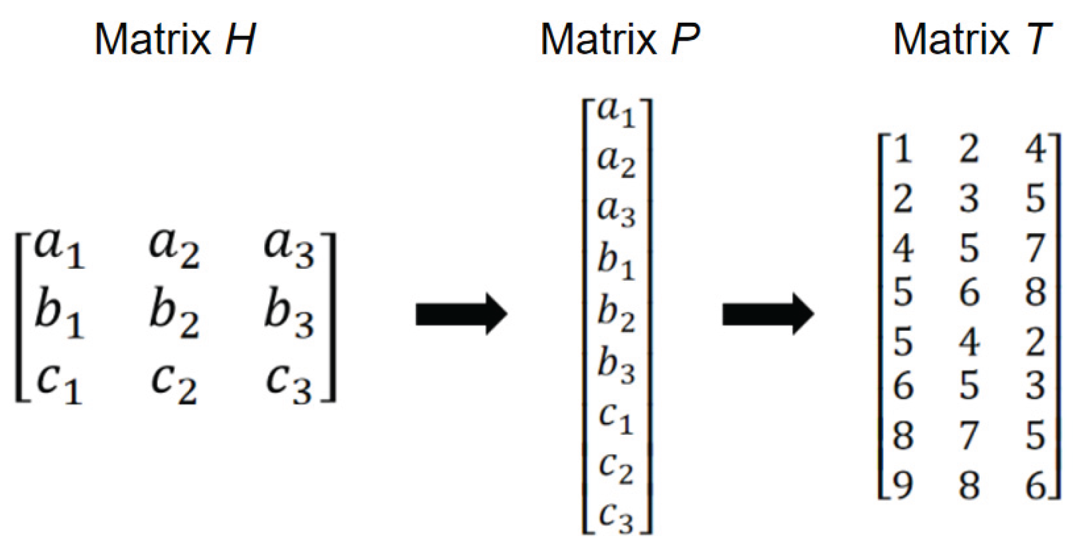
Figure 2.
Process of model segmentation in Blender. (a) Import model file and create a copy; (b) Set segmentation units and construct a rectangular prism cutter; (c) Create and apply a Boolean modifier; (d) Optimize the segmentation results.
Figure 2.
Process of model segmentation in Blender. (a) Import model file and create a copy; (b) Set segmentation units and construct a rectangular prism cutter; (c) Create and apply a Boolean modifier; (d) Optimize the segmentation results.
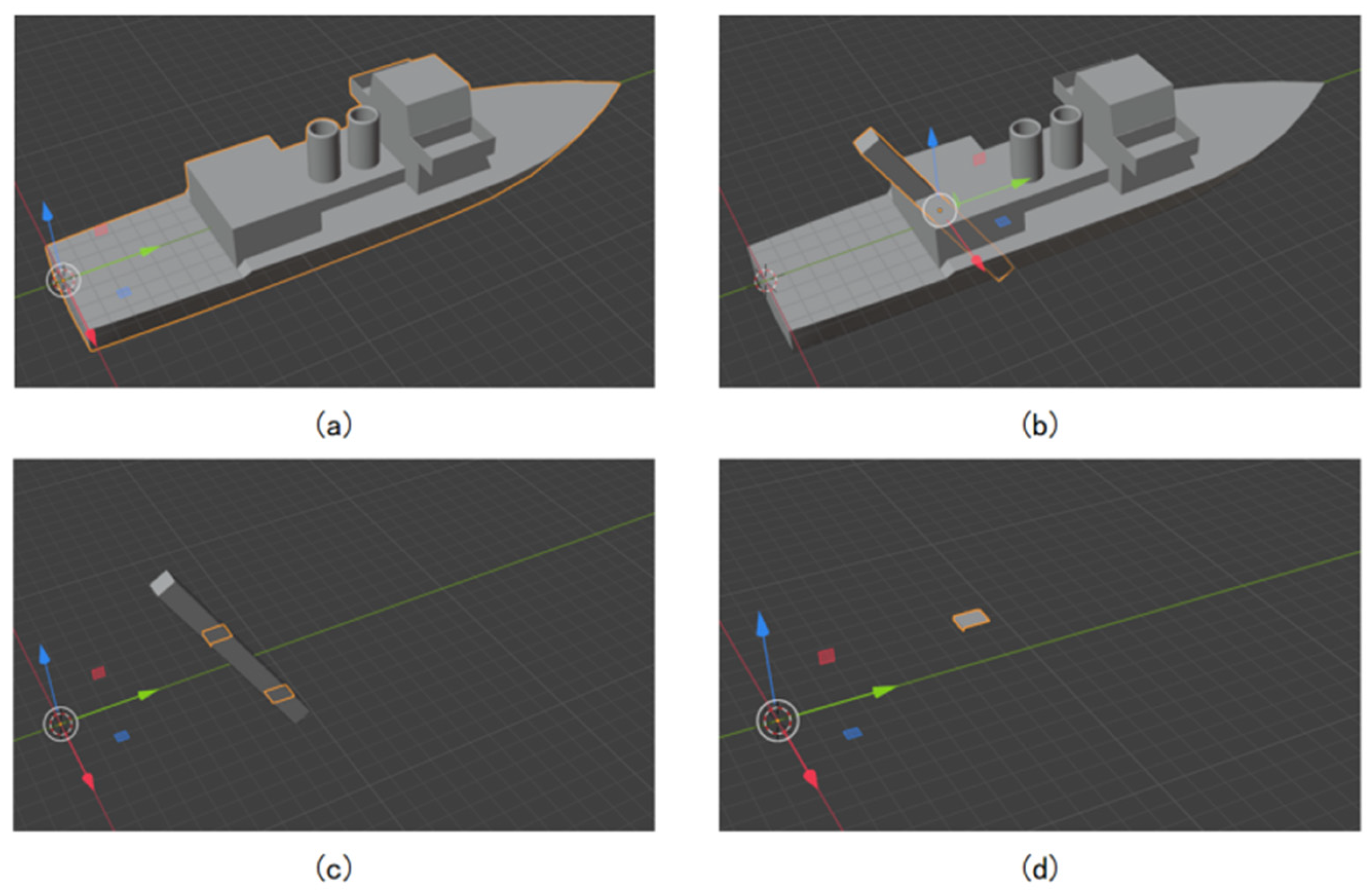
Figure 3.
Schematic of electromagnetic scattering model of the PO method.
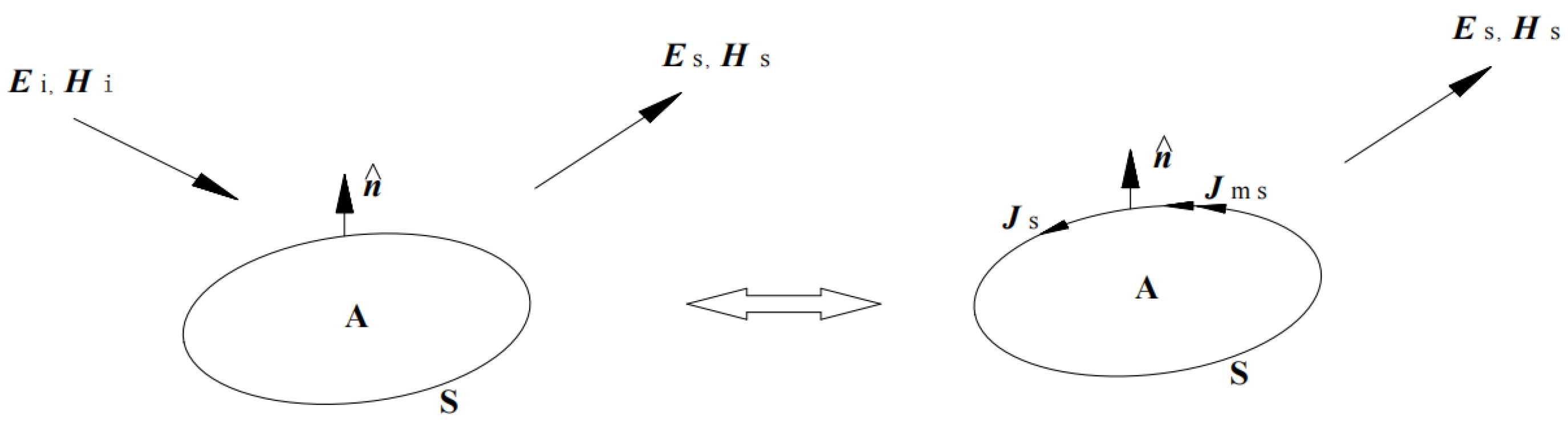
Figure 4.
Simulation results (partial) in the “.out” file.
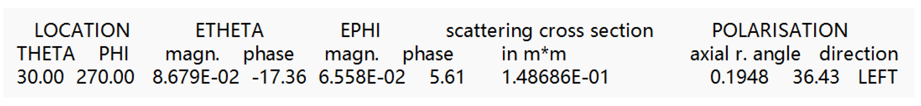
Figure 5.
Flowchart of CS imaging algorithm.
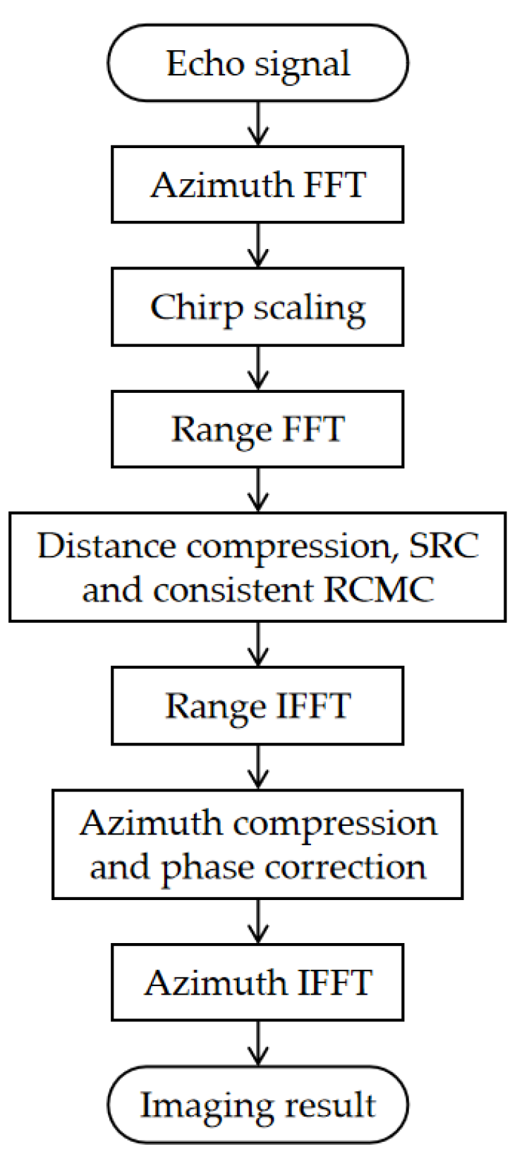
Figure 6.
Sea model of sea conditions ranging from 0 to 5 levels. (a) 0-level sea condition; (b) 1-level sea condition; (c) 2-level sea condition; (d) 3-level sea condition; (e) 4-level sea condition; (e) 5-level sea condition.
Figure 6.
Sea model of sea conditions ranging from 0 to 5 levels. (a) 0-level sea condition; (b) 1-level sea condition; (c) 2-level sea condition; (d) 3-level sea condition; (e) 4-level sea condition; (e) 5-level sea condition.
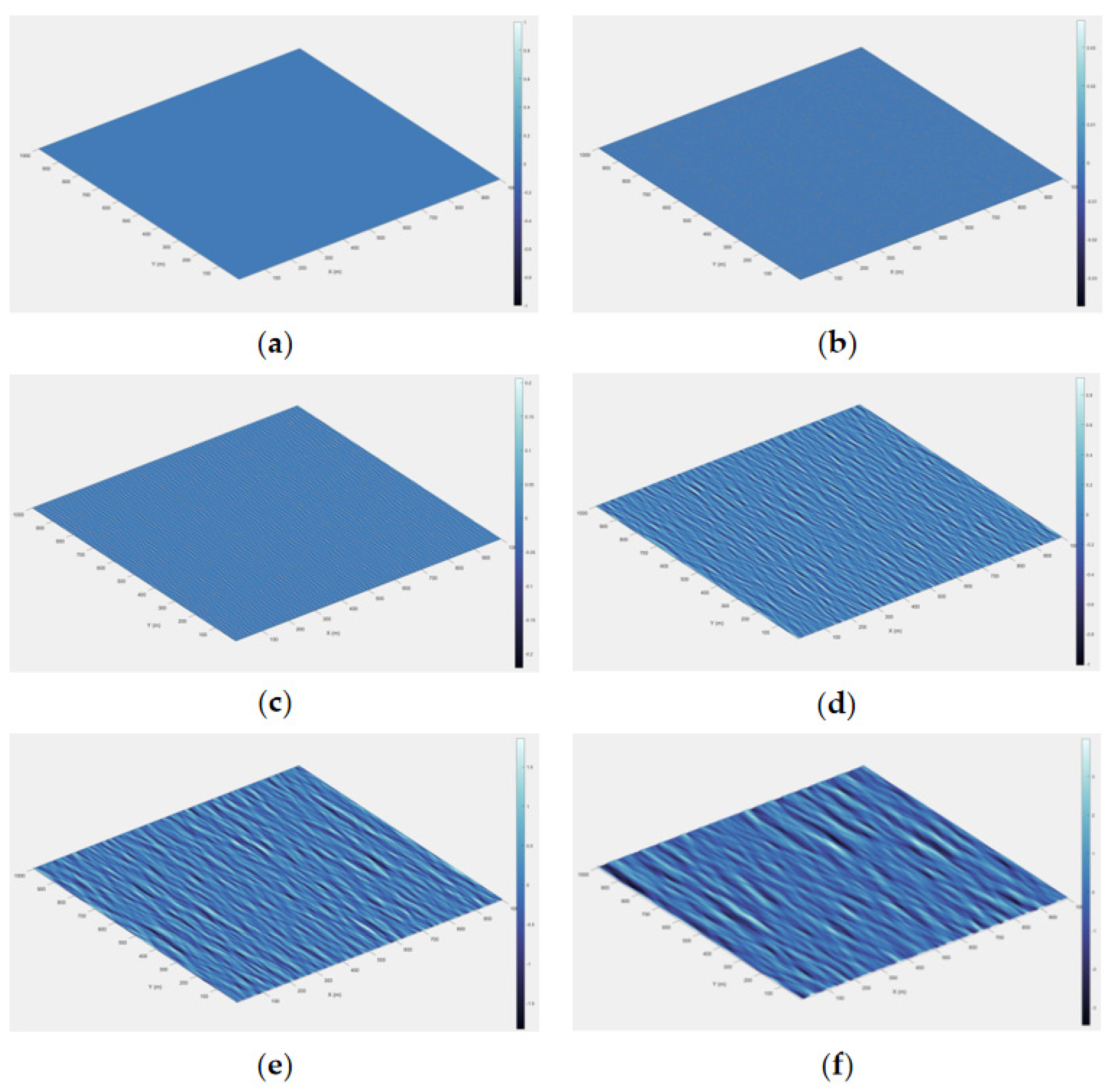
Figure 7.
Change process of the sea model of 3-level sea condition within 0 to 3 seconds. (a)
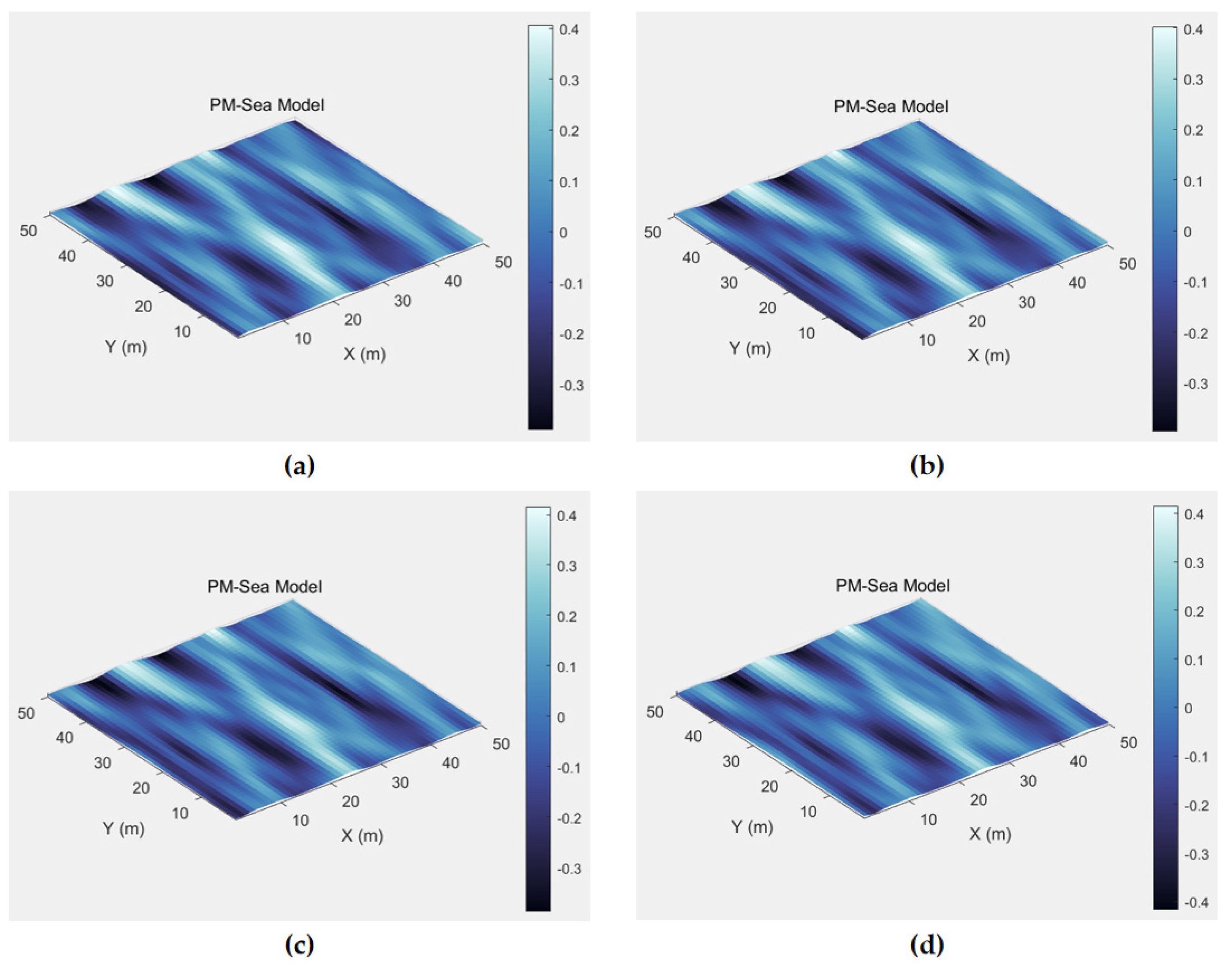
Figure 8.
Complex structure segmentation result. (a) Error segmentation result; (b) Correct segmentation result.
Figure 8.
Complex structure segmentation result. (a) Error segmentation result; (b) Correct segmentation result.
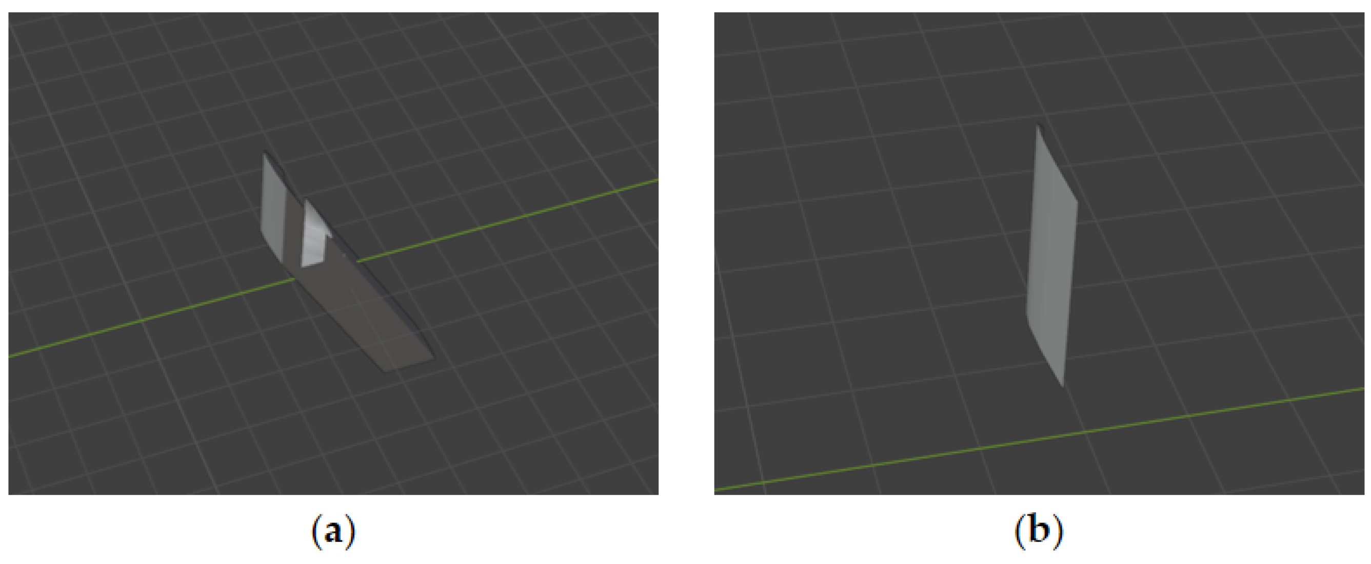
Figure 9.
Comparison of ship target models before and after segmentation. (a) Ship model before division; (b) Ship model after division (assembled).
Figure 9.
Comparison of ship target models before and after segmentation. (a) Ship model before division; (b) Ship model after division (assembled).
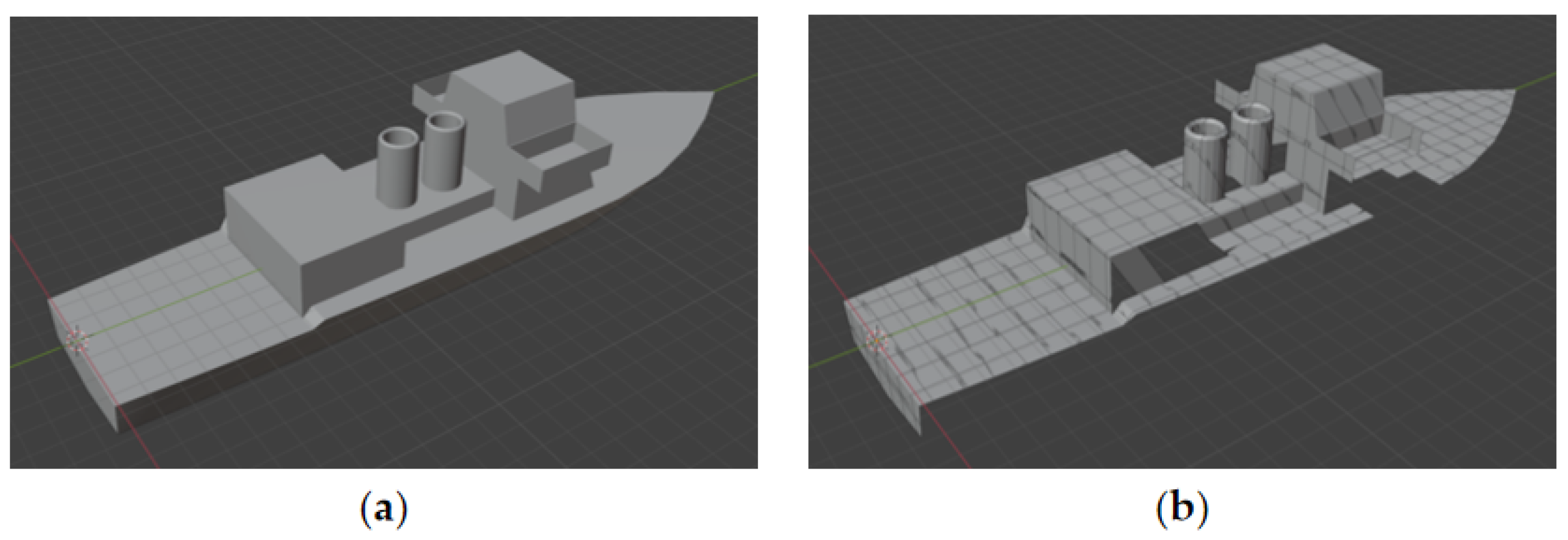
Figure 10.
RCS simulation result of sea model of 3-level sea condition. (a) Complete RCS simulation results; (b) Local enlargement of RCS simulation results; (c) Local enlarged sea model of 3-level sea condition.
Figure 10.
RCS simulation result of sea model of 3-level sea condition. (a) Complete RCS simulation results; (b) Local enlargement of RCS simulation results; (c) Local enlarged sea model of 3-level sea condition.
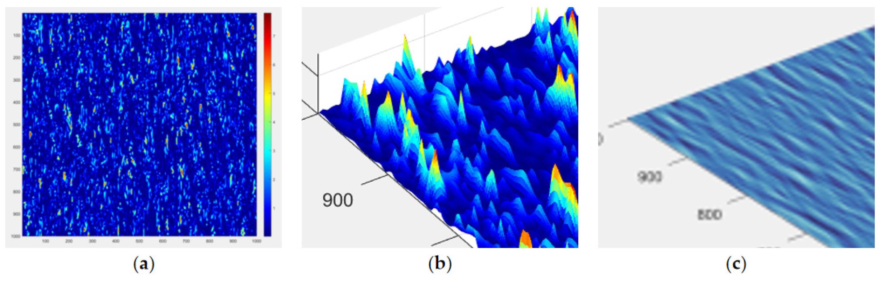
Figure 11.
RCS simulation results of the ship target.
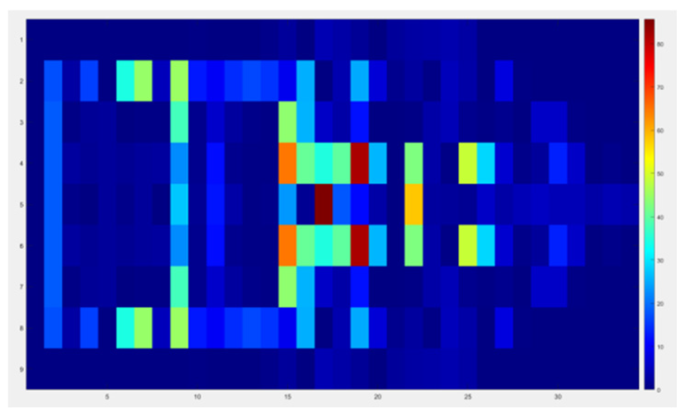
Figure 12.
Point target simulation and imaging results. (a) SAR echo signal of point target; (b) Imaging result of point target.
Figure 12.
Point target simulation and imaging results. (a) SAR echo signal of point target; (b) Imaging result of point target.
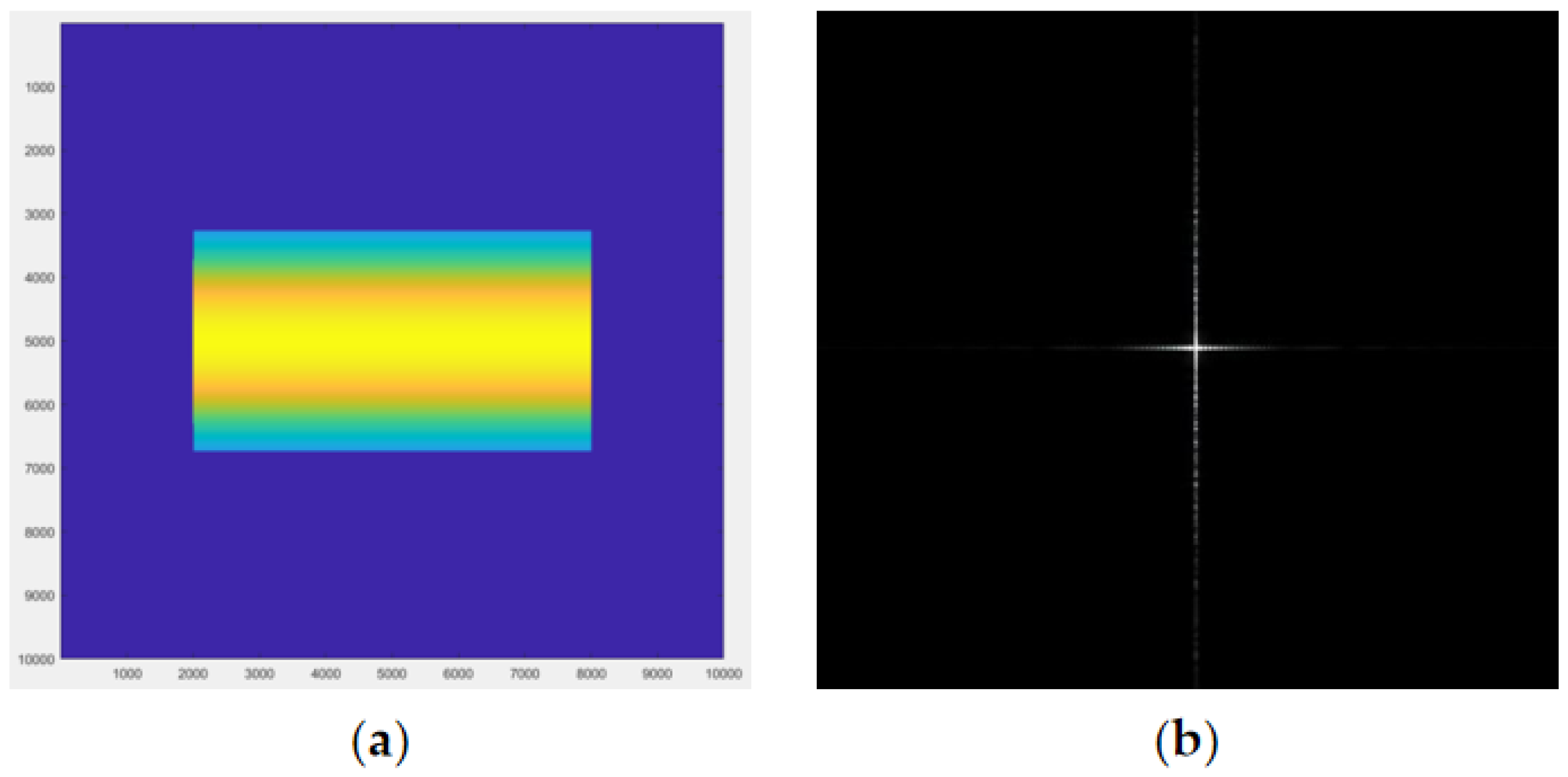
Figure 13.
Assessment results of target quality. (a) Azimuth assessment result; (b) Range assessment result.
Figure 13.
Assessment results of target quality. (a) Azimuth assessment result; (b) Range assessment result.
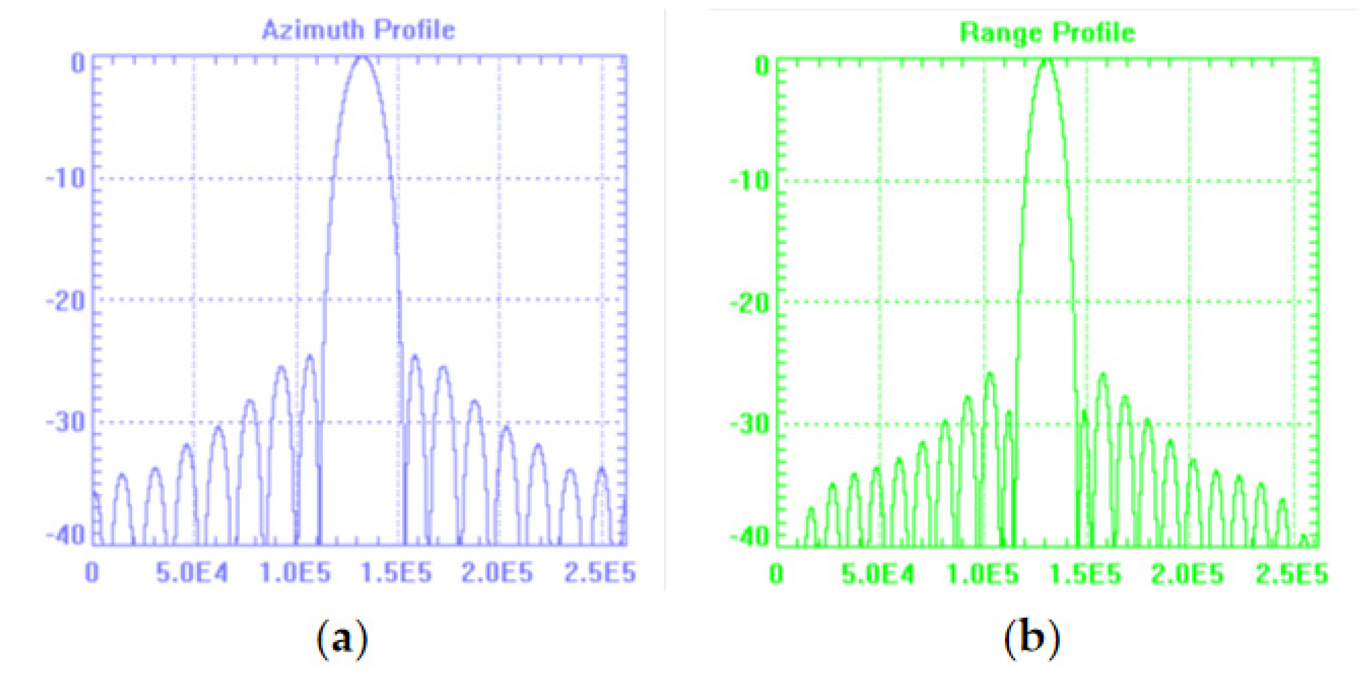
Figure 14.
Simulation and imaging results of ship targets under 3-level sea conditions. (a) SAR echo signals of ship targets under 3-level sea conditions; (b) Imaging result of ship targets under 3-level sea conditions.
Figure 14.
Simulation and imaging results of ship targets under 3-level sea conditions. (a) SAR echo signals of ship targets under 3-level sea conditions; (b) Imaging result of ship targets under 3-level sea conditions.
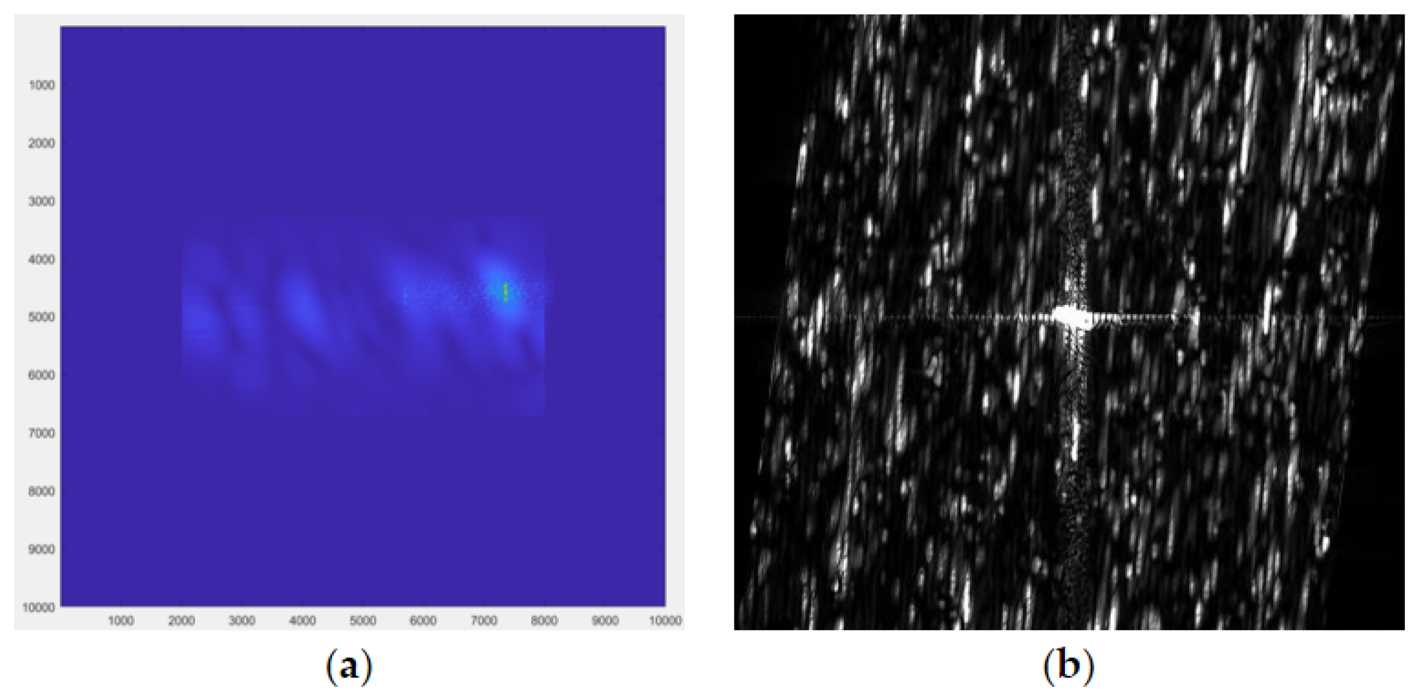

Table 1.
Sea states codes based on Douglas sea scale.
| Code | Characteristics | |
| 0 | 0 | Calm(glassy) |
| 1 | <0.1 | Calm(rippled) |
| 2 | 0.1-0.5 | Smooth(wavelets) |
| 3 | 0.5-1.25 | Slight |
| 4 | 1.25-2.5 | Moderate |
| 5 | 2.5-4 | Rough |
| 6 | 4-6 | Very rough |
| 7 | 6-9 | High |
| 8 | 9-14 | Very high |
| 9 | >14 | Phenomenal |
Disclaimer/Publisher’s Note: The statements, opinions and data contained in all publications are solely those of the individual author(s) and contributor(s) and not of MDPI and/or the editor(s). MDPI and/or the editor(s) disclaim responsibility for any injury to people or property resulting from any ideas, methods, instructions or products referred to in the content. |
© 2026 by the authors. Licensee MDPI, Basel, Switzerland. This article is an open access article distributed under the terms and conditions of the Creative Commons Attribution (CC BY) license (http://creativecommons.org/licenses/by/4.0/).
Copyright: This open access article is published under a Creative Commons CC BY 4.0 license, which permit the free download, distribution, and reuse, provided that the author and preprint are cited in any reuse.


