
Submitted:
20 February 2026
Posted:
27 February 2026
You are already at the latest version
Abstract
Seasonal tropical wetlands such as the Brazilian Pantanal are increasingly threatened by climate change and extreme events, creating a need for robust monitoring tools that capture hydrological dynamics at high spatial and temporal resolution. This study evaluates Sentinel-1 Synthetic Aperture Radar (SAR) imagery to map and monitor flooding within the Ramsar-designated SESC Pantanal Reserve from 2017 to 2020. Ground Range Detected (GRD) VV-polarized scenes were pre-processed with radio-metric terrain normalization and speckle filtering (Lee filter, 5×5 window) to improve separability of water and non-water surfaces. Flooded areas were first extracted using Otsu’s histogram thresholding and validated with high-resolution optical imagery (PlanetScope and Landsat-8). A supervised Random Forest classifier then refined land-cover discrimination into three classes (open water/flood, open land/vegetation, and others), with temporal consistency supported by Cuiabá River hydrological data. Results indicate strong interannual variability in flood extent, with March 2017 inun-dating 34.7% of the reserve compared with 0.75% in March 2020, and peak inundation in April 2017 (79.9%). Overall, Sentinel-1 SAR effectively delineated open water and flooded vegetation under persistent cloud cover, highlighting its value for comple-menting existing products (e.g., MapBiomas), strengthening wetland management, and supporting scalable flood monitoring in other tropical, flood-prone Ramsar sites.
Keywords:
flood
; hydrology
; pantanal
; remote sensing
; wetlands
1. Introduction
Wetlands are ecosystems that face serious threats due, among others, to climate change and other extreme events [1,2]. The Pantanal, as a wetland ecosystem, is influenced by the monomodal flooding cycle, composed of an aquatic and a terrestrial phase [3]. This cycle plays a fundamental role as an ecological factor, being the driving force that characterizes the ecosystem [4]. rivers [5].
The magnitude of floods varies, and this plays a crucial role in determining the degree of connectivity between rivers and their floodplains [6,7]. In the Pantanal, the floodplains have an ecological integrity closely linked to hydrology, meaning the proper functioning of these ecosystems is heavily dependent on flood patterns and the hydrological regime [8]. Monitoring flood dynamics is critical to understanding and managing these systems, which regulates nutrient cycles, vegetation patterns, and habitat availability.
Studies have demonstrated the potential of using SAR (Synthetic Aperture Radar) data to identify and monitor floods in wetland areas [9,10,11]. Some of these studies have focused on using high-resolution data to achieve near real-time monitoring, enabling a rapid response to flood events. Other studies have explored the use of moderate-resolution data, such as those provided by the Sentinel-1 satellite, to monitor floods [12,13,14,15].
These studies have shown encouraging results, highlighting the ability of SAR images to identify flooded areas, map the extent of floods, and monitor changes over time [16,17,18]. The use of SAR data provides a comprehensive and synoptic view of affected areas regardless of atmospheric conditions, as radar can penetrate clouds and operate both day and night. SAR data can provide valuable information about flooded areas, assisting in the monitoring and management of these internationally important wetland ecosystems [19,20].
However, it is important to mention that the accuracy and effectiveness of flood monitoring with SAR data depend on various factors, including data quality, the ability to correct errors and artifacts, correct image interpretation, and integration with other information sources [21].
In this paper, we focused on the potential use of polarimetric SAR data from Sentinel-1. Specifically, we utilized the available Ground Range Detected (GRD) intensity data to map and monitor floods in large wetland areas. Despite their importance, the spatial and temporal dynamics of flooding in the Pantanal remain poorly monitored due to limitations in ground-based data and frequent cloud cover, which constrains the use of optical remote sensing. In this context, Synthetic Aperture Radar (SAR) data especially from Sentinel-1—offers a valuable alternative, with its ability to penetrate cloud cover and detect water surfaces under various conditions.
This information is important for evaluating the suitability of Synthetic Aperture Radar (SAR) data in determining the extent of flooding during flood periods in the Pantanal tropical wetland. Thus, the study answered: (1) the capability of Sentinel-1 images to map and monitor floods, particularly the spatial and temporal patterns of flooding in the Pantanal wetland, and (2) how the hydrological dynamics and rainfall regime are being affected over time. Satellite images were used to analyze the spatial and temporal dynamics, revealing the spectral response of water. The temporal variable allowed for the establishment of a visual pattern in relation to water and the analyzed water bodies.
By improving the understanding of spatial flood variability, this study builds upon the previous publication by Milien et al. (2023) and contributes to the development of effective tools for wetland monitoring and adaptive management.
2. Materials and Methods
2.1. Study Area
The study area is located within the Ramsar SESC Pantanal site (Figure 1), in the northern part of the Pantanal, where the Cuiabá River a major tributary of the São Lourenço River plays a central role in shaping the region’s seasonal flood dynamics. This area is characterized by a peculiar hydroclimatic regime directly influenced by the seasonal cycles affecting this vast wetland area. It has two well-defined climatic seasons: the rainy season and the dry season. During the rainy season, which generally occurs from October to April, rainfall is intense and frequent, resulting in a significant rise in water levels in the Cuiaba River. In the northern Pantanal. The flooding period is from October to December. The flood season, which extends from January to April, is characterized by the peak volume of water, creating a conducive environment for the reproduction of various aquatic species [22].
In the dry season, from May to September, rainfall decreases dramatically, and long periods without precipitation can occur, usually in July and August. The dry period from June to September is marked by a significant reduction in river levels, making previously flooded areas accessible again [6].
The Cuiabá River forms a depositional system that covers an area of 15,300 km2. This region exhibits significant geomorphological complexity, with various types of sedimentary deposits formed by the actions of the Cuiabá River and other rivers in the area. The influence of the Cuiabá River is fundamental in shaping the landscape and functioning of the Pantanal ecosystem, as the transport of sediments and nutrients plays a crucial role in the biodiversity and natural cycles of this region [23].
2.2. Methods
2.2.1. Availability and Selection of Images
Sentinel-1 was launched in 2016; we utilized all available images from the following time intervals: January 2017 to April 2017 and January 2020 to April 2020. This period was chosen due to the highest flood and drought activity observed over the past decade, according to hydrograph data provided by ANA (National Water Agency) [24].
Sentinel-1A and Sentinel-1B operate in a coordinated manner to map the Earth every six days, allowing each satellite to capture the same region every 12 days [25]. The resulting images are available at different processing levels, already calibrated and georeferenced using the Sentinel-1 Toolbox. These images can be accessed for free at the Copernicus Open Access Hub (https://scihub.copernicus.eu/dhus/#/home).
Both Sentinel-1A and Sentinel-1B are equipped with a C-band SAR (Synthetic Aperture Radar) system (with a frequency of 5.405 GHz) and have the capability to acquire polarimetric SAR data in Interferometric Wide (IW) mode (Twele et al., 2016). These GRD (Ground Range Detected) images have a spatial resolution of 10 meters and are acquired in IW mode [26].
We used the C-band GRD product from Sentinel-1 to extract backscatter information from the images to identify flooded areas. Specifically, we opted for the vertical-vertical (VV) co-polarization mode, which provides suitable backscatter intensity values for wetland areas [27]. Horizontal-horizontal co-polarization has shown greater accuracy than vertical-horizontal polarization and other co-polarization modes for detecting floods in wetland areas [28].
2.2.2. Pre-Processing
The Sentinel-1 images underwent a series of preprocessing steps to ensure data accuracy and quality. These preprocessing steps included the calibration of the backscatter coefficient (sigma0) in decibels (dB), thermal noise removal, data calibration, and Range-Doppler terrain correction [29,30].
To maximize information extraction, we performed additional preprocessing of Sentinel-1 images for speckle filtering and radiometric terrain normalization using SNAP software [29]. These additional steps aim to reduce the effect of speckle noise on the images and enhance radiometric consistency across different terrain areas.
2.2.3. Speckle Filtering
Inherently, SAR images are affected by speckle noise. The speckle effect results from the interference of many scattering echoes within a resolution cell [31]. Speckles degrade the quality of image data and interfere with understanding the backscattering responses of surface features. Speckle filtering is an essential part of preprocessing activities in SAR products [32].
The principle of speckle filtering is to reduce the variation of complex speckles and improve the estimation of the scattering coefficient. In this study, the Lee filter with a 5x5 window was applied to Sentinel-1 images to reduce speckle noise, a common issue in Synthetic Aperture Radar (SAR) data that can obscure fine features crucial for flood monitoring. The 5x5 window size offers an optimal balance between noise reduction and detail preservation, effectively smoothing out noise while retaining critical landscape features, such as the boundaries of flooded areas. This choice is particularly suitable for monitoring the Pantanal, where seasonal flooding demands accurate delineation of water bodies. The Lee filter enhances the interpretability of water versus non-water areas in the SAR data, making it easier to create reliable flood history records. Additionally, using a 5x5 window aligns with established practices in SAR-based flood studies. The Lee filter is a particular case of the Kuan filter, which filters based on the criterion of minimum mean squared error (MMSE). These speckle filters range from a simple blind low-pass filter, such as the boxcar filter, to different adaptive filters, such as the Lee filter (Lee, 1980), the Maximum A-posterior (MAP) Gamma filter [33], the refined Lee filter [34], and the enhanced sigma Lee filter [35].
2.2.4. Radiometric Terrain Normalization
Radiometric normalization for terrain effect correction is a critical step that requires clear justification and detailed explanation, especially in regions where topography can significantly influence SAR backscattering results [36] . This correction is necessary due to the side-looking nature of SAR systems, which map each target on the terrain in the slant range domain [37]. Although Sentinel-1 images available as GRD are already corrected for geometric distortions, radiometric terrain normalization was applied to ensure data accuracy in areas prone to topographic variations. This normalization process masks pixels in regions of active overlap and shadow within the images [38].
In the Pantanal, which has relatively flat topography, topographic effects are less pronounced compared to mountainous areas. However, radiometric normalization remains relevant, as even slight elevations can interfere with radiometric measurements in low-slope environments. For this step, angle-based correction methods were used: one based on volume scattering and the other on surface scattering [20].
For radiometric terrain normalization, there are two angle-based correction methods, one based on volume scattering and the other on surface scattering [30]. The volume scattering model is important for vegetation mapping applications. For wetland applications, as in our case, the surface scattering model based on angles is more appropriate [30].
2.2.5. Water and Non-Water Surface Separation (Binarization)
To identify flooded areas, it is crucial to distinguish between water and non-water surfaces using the binarization technique. Histogram thresholding is one of the most used techniques to convert single-band value images into two distinct classes, such as target and “background”[39]. However, choosing an appropriate threshold is a crucial and challenging step to achieve accurate and reliable binarization. In image analysis, it is necessary to objectively and automatically determine a single threshold to distinguish two relatively homogeneous features in a single-band image, such as land and water, which exhibit a bimodal distribution of pixels.
In this study, we used the Otsu method for image segmentation [40]. The Otsu method is an automatic image binarization technique based on histogram thresholding. It provides a means to automatically find an optimal threshold based on the observed distribution of pixel values. The Otsu method aims to segment an image by minimizing intra-class variation between two distinct homogeneous classes, using a histogram-based approach. The histograms of these classes represent different ranges of intensity values, and the method divides the histogram into two groups using a threshold determined by minimizing the weighted variation between the two homogeneous classes.
The following equation was used to achieve this minimization of intra-class variation [41].
The formula to find the threshold in the Otsu method is based on maximizing the interclass variance, which is equivalent to minimizing the sum of intra-class variances. The interclass variance is defined as follows: interclass variance = p1 * p2 * (mean1 - mean2) ^2, where p1 and p2 are the probabilities of the two classes divided by the threshold, whose value ranges from 0 to 255, and (t) represents the threshold. The means (mean1 and mean2) are the intensity means of the two classes.

The goal is to find the threshold that maximizes this interclass variance to obtain the desired segmentation.
The average digital number in class k, denoted by µk, is calculated as the mean of pixel values belonging to that class. The average digital number of the entire dataset is represented by l. Class k is defined by each class value less than a certain threshold t. In this context, we are estimating the threshold that maximizes the Between-Class Sum of Squares (BSS). Since we have two classes (water and land), the value of p is equal to 2. The BSS is calculated using the following formula [42].

The formula describing the calculation of BSS involves several variables. The variable i refers to the observations (pixels) in each class, j refers to the classes (water and non-water), and ni represents the number of observations in class i. The variable C denotes the global mean of the values, with VV being the specific variable under consideration (e.g., intensity). The class mean (µk) and the global mean (C) are used in the calculation of BSS.
The global mean C is denoted as follows:

The cluster probability calculation equation is used for each separate cluster, whether water or non-water. This equation is represented as follows: Probability = The cluster probability calculation equation is used for each separate cluster, whether water or non-water. This equation is represented as follows:
where ( n_i ) is the number of observations in the specific cluster and \( N \) is the total number of observations in all classes (water and non-water). This probability represents the proportion of the cluster relative to the total dataset. It is a relative measure that indicates the presence of a particular cluster relative to all observations.
where (ni) is the number of observations in the specific cluster and (N) is the total number of observations in all classes (water and non-water). This probability represents the proportion of the cluster relative to the total dataset. It is a relative measure that indicates the presence of a particular cluster relative to all observations.
In the cluster probability calculation equation, p(i) represents the probability of the specific cluster, where p(i) is calculated as the ratio of the number of observations in the cluster (n_i) to the total number of pixels in the image (n). This probability p(i) indicates the proportion of the cluster relative to the total number of pixels in the image. It is a relative measure that reflects the presence of the specific cluster relative to the complete set of pixels in the image.
2.2.6. Field Validation
In the literature, the confusion matrix is widely used as a measure of accuracy evaluation, which was employed to estimate the accuracy of binarization for separating water and land. For this purpose, randomly generated point observations were used as a test set. The classes of the ground truth points were determined based on the visual interpretation of high-resolution optical images (Planet scope with approximately 3 m resolution) and Landsat-8 images captured in Google Earth. In total, 150 water truth points and 150 non-water truth points were identified. The VV backscattering of different features, such as buildings, channel beds, floodplains, and water bodies, was analyzed in sampling areas within and around the SESC Pantanal Ramsar Site to better understand the spectral confusion between these features, which will be discussed in the next section of this study.
2.2.7. Accuracy
A Random Forest classifier was trained to map three land-cover classes (water/flood, open land, and others) and was evaluated using cross-validation and an independent testing dataset. Overall performance on the testing dataset was high, with 97.70% correct predictions (n = 6622), RMSE = 0.2396, and a small bias = −0.0187. Class-wise accuracy and precision were consistently high across classes, although the open land class was under-represented in the testing data (2.17%), which can affect per-class uncertainty. Full confusion-matrix statistics (TP/FP/TN/FN), class distribution, and feature-importance results are provided in the Supplementary Material.
2.2.8. Hydro-Climatic Data
To define the timing and magnitude of floods in the study area, we used rainfall and river flow data from the National Water Agency (ANA), which were obtained from the agency’s website (https://www.snirh.gov.br/hidroweb/serieshistoricas) (accessed on October 23, 2023). Since our study area is delimited by the Cuiabá River, it was necessary to download river flow data for it. The chosen station was Porto Cercado on the Cuiabá River (river gauge station code 66340000 and rainfall station code 1656001).
3. Results
3.1. Hydrological and Rainfall Patterns at the Porto Cercado Station (2017–2020) Variability of the Cuiabá River
Hydroclimatic data from the Porto Cercado fluviometric station located upstream of the SESC Pantanal Ramsar Site on the Cuiabá River were analyzed to characterize river discharge and precipitation patterns between 2017 and 2020 (Figure 2). The highest average monthly discharge during the study period was recorded in March 2017, reaching 603 m3/s. In subsequent years, peak discharges occurred in April, with similar magnitudes: 595 m3/s in 2018 and 588 m3/s in 2019. A marked reduction in river discharge was observed in 2020, with the annual maximum reaching only 488 m3/s. The lowest discharge of the entire period was recorded in September 2020, at 150 m3/s, indicating severe low-flow conditions [8,43].
Precipitation data show that the highest monthly rainfall occurred in February 2018 (280 mm). As expected for the regional climate, maximum rainfall typically occurred between November and February. However, the 2019–2020 wet season exhibited anomalously low precipitation (peak of 230 mm), deviating from historical norms and contributing to reduced flood magnitudes observed in that year. It is important to note that monthly rainfall data for August 2017 were not available in the ANA dataset, representing a minor data gap in the time series.
Figure 3 illustrates, during the months of January to April 2017, the flooded areas. The dark blue regions represent permanent water bodies: areas where water is present in all observations, including the main tributaries of the Cuiabá River that flow. It can be observed that the degree of flooding in the Ramsar SESC Pantanal site varies between flood months: in March, coinciding with the peak flow, practically the entire reserve is flooded. In January, the flooded area is smaller than in March but larger than February and April, suggesting that accumulated rainfall in the area is a significant factor in flooding. However, despite the flows in February and April being important (522 and 598 m3/s respectively), the flooded area is much smaller than in March or January, which suggests that other factors may intervene in the flooding process.
3.2. Temporal Variation of Flooded Areas Estimated Using the Binarization Linear Method (2017–2020)
Table 1 presents the variation in flooded areas over different periods using a linear binarization method. The results show significant temporal fluctuations in flood extent, reflecting hydrological variability within the study area. The most extensive flooding occurred in March 2017, where open water bodies covered 37,509.8 hectares, accounting for 34.7% of the study area. This suggests a major hydrological event, likely driven by increased precipitation, seasonal river discharge, or other hydrometeorological factors. Similarly, January 2017 recorded a substantial flooded area of 11,619.6 ha (10.75%), indicating another period of elevated water levels.:
In contrast, the lowest recorded extent was in September 2020, with only 73.5 ha of open water detected. This minimal flooding could be attributed to seasonal dry periods, reduced precipitation and lower river discharge. Other periods with relatively low flooding include September 2017 (426.4 ha, 0.39%), January 2020 (1037.0 ha, 0.96%), and March 2020 (809.3 ha, 0.75%), indicating similar low-water conditions.
A pronounced fluctuation is evident between different years and seasons. For instance, while March 2017 exhibited extreme flooding, March 2020 displayed a significantly lower extent (809.3 ha, 0.75%), indicating interannual differences in hydrological drivers. The April 2017 (1218.1 ha, 1.13%) and February 2017 (1731.4 ha, 1.60%) values suggest that flooding was minimal in those months compared to January and March of the same year. Additionally, September consistently records lower flood extents across years (2017 and 2020), implying a recurrent seasonal pattern of reduced water levels.
3.3. Random Forest Classification
The random forest classification maps (Figure 4) illustrate the spatial distribution of flooded areas, open land, and other land cover types from January to April 2017. The classification results distinguish three major land cover categories which include both seasonally and permanently flooded areas; Open Land | Vegetation, which consists of wetlands, and sparsely vegetated areas. The map shows a clear seasonal variation in flooding, with January and March exhibiting moderate flood extents, while April records the highest inundation area. In contrast, February presents the lowest flood extent, despite moderate river discharge, suggesting that local rainfall, soil saturation, and floodplain retention capacity play a key role in controlling seasonal flooding dynamics.
The quantitative assessment of flooded areas derived from the random forest classification further supports the observed seasonal patterns (Table 2). In January 2017, approximately 11,619.69 hectares (10.75%) of the study area was flooded. However, flood extent significantly decreased in February to only 831.13 hectares (0.77%), making it the month with the lowest recorded flood extent. A substantial increase was observed in March, where 37,509.80 hectares (34.70%) were flooded, indicating the transition toward peak inundation. Finally, April recorded the highest flood extent, with 86,433.10 hectares (79.96%) of the area underwater, representing the most extensive flood event of the study period. The results suggest that while river discharge contributes to flooding, other hydrological factors, such as accumulated precipitation and floodplain retention, play a crucial role in determining the extent of water coverage in different months.
The peak flood in April ensures high hydrological connectivity, allowing for nutrient transport and sediment deposition, which are critical for maintaining floodplain productivity (REF). Despite moderate river discharge in February (522 m3/s) and April (598 m3/s), February exhibited the lowest flood extent, emphasizing that flood patterns are not solely dictated by river discharge.
We performed a Kruskal-Wallis test to determine whether there are significant differences in the Area variable across the three land cover classes: “Water|Flood”, “Open_Land|Vegetation”, and “Others”. The test statistic obtained was χ2 = 0.34615 with 2 degrees of freedom. This chi-squared value represents the degree to which the ranks of the different groups deviate from what would be expected under the null hypothesis, which assumes no differences between groups.
The p-value associated with this test was 0.8411. A p-value represents the probability of obtaining test statistics as extreme as the one observed, assuming that the null hypothesis is true. Since this p-value is much larger than the common significance threshold of 0.05, it indicates that there is no strong evidence to suggest significant differences in the distribution of Area values across the three land classes.
4. Discussion
The application of Sentinel-1 aimed to overcome limitations was found with the use of other remote sensing products. However, we assert that Sentienl-1 may serve as tools for flood monitoring in wetlands, specifically because several challenges have been reported regarding cloud cover and the complex spectral conditions of lake water when only optical data are used [24]. Diverse studies using MODIS data [44,45] reported limitations due to low spatial resolution, while comprehensive information was obtained based on high temporal resolution [46,47].
By contrast, the following advantages of Sentinel-1, used in this study, can be clearly highlighted: i) the high spatial resolution of Sentinel-1 data (10 meters), which allows for a detailed spatial analysis of water surface patterns and related flooded areas, ii) the temporal resolution of the Sentinel-1 time series allows for monthly assessments of flooded areas, and iii) the water extent obtained by Sentinel-1 provides continuous information from an active sensor, available even during cloudy periods [12,48].
Thus, these advantages of Sentinel-1 are highlighting that the two parts of the reserve (Paleo-area and recent area) [5]) are flooded at different times. This flooding phenomenon can be caused by both local rains and water from the São Lourenço and Cuiabá rivers, which enter through underground channels, surface channels, and artificial channels [3].
It is important to note that there are variations in the flood phases in the different sub-regions of the study area, as well as the possibility of multi-year variations of more intense floods or droughts. The drought and fire events in the Pantanal in 2020 received wide coverage in national and international media. The periodic repetition of drought and fire periods in the Pantanal is predicted by mathematical models [49,50].
These analyzes suggest that the pattern of intense droughts is moving towards a new climatic scenario in the Pantanal, which is in line with the projections of mathematical models [51,52]. This shift has ecological implications, including the loss of ecological connectivity, interruption of life cycles for aquatic fauna, and reduced regeneration of hydrophilic vegetation. Sentinel-1, as a continuous monitoring tool, enables detection of such hydrological anomalies and long-term climate-driven changes.
Hence, our findings have direct implications for the adaptive management of the Ramsar Sítio SESC Pantanal. The flood information derived from Sentinel-1 can support the development of early warning systems, especially for drought-prone areas, and inform management plans for conservation units such as Private Natural Heritage Reserves (RPPNs) and Legal Reserves.
Moreover, flood extent data are useful for identifying and monitoring critical aquatic habitats. In the context of the Ramsar Convention, this evidence contributes to ecological character descriptions, indicators for monitoring wetland health, and land use zoning strategies. These applications align with public policies for wetland sustainability and ecosystem-based management.
To complement the flood frequency maps of the Pantanal from the data sources presented by MapBiomas 2020 collections, Sentinel-1 data can provide additional spatial information. This allows differentiation of details related to natural structures of flooded areas, such as potential habitats for aquatic birds located in lakes and dynamically changing small areas [53], as well as structures of flooded areas created by humans, such as narrow channels, to maintain water in the landscape as an adaptation strategy to climate change.
In comparison with the MapBiomas 2020 time series dataset, although it has a much lower temporal resolution, the flood frequency derived with Sentinel-1 shows very good agreement in the flooding pattern [54]. However, as can be seen in the differences in Figure 2, ANA’s monthly data may reveal flooding that cannot be detected by Sentinel-1 during very dynamic flood periods due to higher temporal resolution. Combining the advantages of both data sources for flood mapping is a future task that could result in even better monitoring results.
Future research should explore coupling SAR-derived flood data with hydrological, topographic, and climate models to enhance predictions of flood scenarios under changing environmental conditions. The use of multivariate machine learning algorithms is also encouraged to increase the classification accuracy of seasonally flooded wetlands and improve the detection of ephemeral flood patterns.
The maps demonstrate that the Sentinel-1 backscattering in VV polarization was approximately 13 dB (decibels) higher in the flooded area than in the open water. Therefore, this polarization is useful for distinguishing between open water, flooded area, and dry area (Huang & Jin, 2022). The lower backscattering in VV for open water, at least 10 dB lower than all classes of flooded vegetation, makes it the preferred image for mapping open water. The C-band in VH polarization is not useful for distinguishing open water from flooded pasture and submerged vegetation [55].
Therefore, the C-band in VV and VH is useful for separating flooded areas with different types of vegetation. However, VH polarization is more effective than VV in discriminating between vegetation and flooded pasture because the difference between vegetation and flooded pasture is greater in VH (at least 10 dB) than in VV (~ 5 dB). Additionally, both VV and VH polarizations can be beneficial for differentiating submerged vegetation from dense and sparse vegetation (VH submerged = 10 dB and VV submerged-emergent = 10 dB) (Tuan et al., 2021).
The use of Synthetic Aperture Radar (SAR) data is a promising approach to answer questions and investigate the hydrological dynamics of flooded environments. The use of the Sentinel-1 SAR image series is a valuable option for flood mapping in areas with large water flow, such as the Pantanal. However, it is important to be aware of the challenges associated with this type of analysis. Speckle noise is a common problem in SAR images, resulting in spots and scatterings that make flood detection difficult, especially in areas with narrow channels in floodplains
Despite such limitations, the integration of SAR (e.g., Sentinel-1) with optical sensors (e.g., Sentinel-2, PlanetScope) and land use/land cover products (e.g., MapBiomas) can provide a more complete picture of hydrological dynamics. These multi-source approaches allow for distinguishing between natural flooding patterns and anthropogenic interventions, improving ecosystem assessments.
5. Conclusions
Sentinel-1 outperforms previous methods such as MODIS by offering higher spatial resolution (10 m) and suitable temporal coverage for monthly flood assessments. It reveals distinct flooding patterns driven by local rainfall and river discharges, providing crucial insights for sustainable water management. In addition, the detailed spatial data capture both natural structures and man-made channels, expanding our understanding of flood behavior. Integrating Sentinel-1 with other data sources (e.g., MapBiomas) confirms consistent flooding patterns, highlighting the power of multi-source approaches. During extreme events, Sentinel-1 provides near-real-time clarity on water expansion and retreat, a level of detail previously unattainable. Overall, this research underscores the utility of Sentinel-1 in distinguishing open water, flooded terrain, and dry areas, establishing a strong foundation for enhanced monitoring and management strategies in the Pantanal Ramsar Site and other biodiversity conservation units
Author Contributions
Conceptualization, Edelin Jean Milien. and Catia Nunes Da Cunha.; methodology Edelin Jean Milien, Catia Nunes da Cunha.; software, Edelin Jean Milien.; validation, Catia Nunes Da Cunha., Pierre Girard. and Edelin Jean Milien.; formal analysis, Edelin Jean Milien.; investigation, Edelin Jean Milien.; data curation, Edelin Jean Milien writing—original draft preparation, Edelin Jean Milien.; writing—review and editing, Edelin Jean Milien, Catia Nunes Da Cunha, Girard Pierre.; visualization, Catia Nunes Da Cunha, Girard Pierre.; supervision, Catia Nunes Da Cunha.; project administration, Edelin Jean Milien.; funding acquisition, Edelin Jean Milien. All authors have read and agreed to the published version of the manuscript.
Funding
Please add: This research was funded by the Coordenação de Aperfeiçoamento de Pessoal de Nível Superior “Capes” through a partnership with GCUB-OAS-PAEC for researcher mobility in ecology and biodiversity conservation at the Federal University of Mato-Grosso. grant number [8887.495657/2020-00].
Acknowledgments
This work was conducted during my philosophy of doctorate (Ph.D) degree study in Ecology and Biodiversity Conservation at the Federal University of Mato-Grosso - UFMT. Funding was provided by the Coordenação de Aperfeiçoamento de Pessoal de Nível Superior “Capes”, through a partnership between GCUB-OAS-PAEC, for researcher mobility. The authors want to thank INAU – CPP (Instituto Nacional de Ciência e Tecnologia em Áreas Úmidas) for their assistance and material support.
Conflicts of Interest
The authors declare that they have no known competing financial interests or personal relationships that could have appeared to influence the work reported in this paper.
References
- Salimi, S.; Almuktar, S.A.A.A.N.; Scholz, M. Impact of Climate Change on Wetland Ecosystems: A Critical Review of Experimental Wetlands. J. Environ. Manage. 2021, 286, 112160. [Google Scholar] [CrossRef]
- Wetlands., R.C. on Ramsar Convention on Wetlands. (2018). Global Wetland Outlook: State; Dudley, N.,Ed.; State of t.; Ramsar Convention Secretariat. Coordinating: Swizerland, 2018.
- Nunes da Cunha, C.; Piedade, M.T.F.; Junk, W.J. Classificação e Delineamento Das Áreas Úmidas Brasileiras e de Seus Macrohabitats; 2015; Vol. 1, ISBN 9788578110796. [Google Scholar]
- Junk, W.J.; Bayley, P.B.; Sparks, R.E. The Flood Pulse Concept in River-Floodplain Systems. Can. J. Fish. Aquat. Sci. 1989, 106. [Google Scholar]
- Pupim, F.D.N. Geomorfologia e Paleo-hidrologia dos Megaleques dos rios Cuiabá e São Lourenço, Quaternário da bacia do Pantanal; Universidade Estadual Paulista: Rio Claro, 2014. [Google Scholar]
- Chen, X.; Chen, L.; Stone, M.C.; Acharya, K. Assessing Connectivity between the River Channel and Floodplains during High Flows Using Hydrodynamic Modeling and Particle Tracking Analysis. J. Hydrol. 2020, 583, 124609. [Google Scholar] [CrossRef]
- Suizu, T.M.; Latrubesse, E.M.; Bayer, M. The Role of Geomorphology on Flood Propagation in a Large Tropical River: The Peculiar Case of the Araguaia River, Brazil. Water (Switzerland) 2023, 15. [Google Scholar] [CrossRef]
- Girard, P. Hydrology of Surface and Groundwaters in the Pantanal Floodplains. Pantanal Ecol. Biodivers. Sustain. Manag. a large Neotrop. Seas. Wetl. 2011, 103–126. [Google Scholar]
- Costa, M.P.F.; Telmer, K.H. Utilizing SAR Imagery and Aquatic Vegetation to Map Fresh and Brackish Lakes in the Brazilian Pantanal Wetland. Remote Sens. Environ. 2006, 105, 204–213. [Google Scholar] [CrossRef]
- González-González, A.; Villegas, J.C.; Clerici, N.; Salazar, J.F. Spatial-Temporal Dynamics of Deforestation and Its Drivers Indicate Need for Locally-Adapted Environmental Governance in Colombia. Ecol. Indic. 2021, 126, 107695. [Google Scholar] [CrossRef]
- Penatti, N.C.; de Almeida, T.I.R.; Ferreira, L.G.; Arantes, A.E.; Coe, M.T. Satellite-Based Hydrological Dynamics of the World’s Largest Continuous Wetland. Remote Sens. Environ. 2015, 170, 1–13. [Google Scholar] [CrossRef]
- Bioresita, F.; Puissant, A.; Stumpf, A.; Malet, J.P. A Method for Automatic and Rapid Mapping of Water Surfaces from Sentinel-1 Imagery. Remote Sens. 2018, 10. [Google Scholar] [CrossRef]
- Pereira, G.H. de A.; Júnior, C.C.; Fronza, G.; Cecchini, F.A.; Deppe. Multitemporal Analysis of SAR Images for Detection of Flooded Areas in Pantanal. RA’E GA - O Espac. Geogr. em Anal. 2019, 46, 88. [Google Scholar] [CrossRef]
- Rosenqvist, J.; Rosenqvist, A.; McDonald, K.C. An Analysis of ICESat-2, PALSAR-2 and Sentinel-1 Data for the Assessment of Inundation Characteristics in the Amazon Basin. Int. Geosci. Remote Sens. Symp. 2020, 5081–5084. [Google Scholar] [CrossRef]
- Zhang, M.; Lin, H. Wetland Classification Using Parcel-Level Ensemble Algorithm Based on Gaofen-6 Multispectral Imagery and Sentinel-1 Dataset. J. Hydrol. 2022, 606, 127462. [Google Scholar] [CrossRef]
- Montalti, R.; Solari, L.; Bianchini, S.; Del Soldato, M.; Raspini, F.; Casagli, N. A Sentinel-1-Based Clustering Analysis for Geo-Hazards Mitigation at Regional Scale: A Case Study in Central Italy. Geomatics, Nat. Hazards Risk 2019, 10, 2257–2275. [Google Scholar] [CrossRef]
- Shen, X.; Wang, D.; Mao, K.; Anagnostou, E.; Hong, Y. Inundation Extent Mapping by Synthetic Aperture Radar: A Review. Remote Sens. 2019, 11, 1–17. [Google Scholar] [CrossRef]
- Townsend, P.A. Mapping Seasonal Flooding in Forested Wetlands Using Multi-Temporal Radarsat SAR. Photogramm. Eng. Remote Sensing 2001, 67, 857–864. [Google Scholar]
- Evans, T.L.; Costa, M.; Tomas, W.M.; Camilo, A.R. Large-Scale Habitat Mapping of the Brazilian Pantanal Wetland: A Synthetic Aperture Radar Approach. Remote Sens. Environ. 2014, 155, 89–108. [Google Scholar] [CrossRef]
- Evans, T.L.; Costa, M.; Telmer, K.; Silva, T.S.F. Using ALOS/PALSAR and RADARSAT-2 to Map Land Cover and Seasonal Inundation in the Brazilian Pantanal. IEEE J. Sel. Top. Appl. Earth Obs. Remote Sens. 2010, 3, 560–575. [Google Scholar] [CrossRef]
- Lu, D.; Weng, Q. Use of Impervious Surface in Urban Land-Use Classification. Remote Sens. Environ. 2006, 102, 146–160. [Google Scholar] [CrossRef]
- Da Silva, C.J.; Girard, P. New Challenges in the Management of the Brazilian Pantanal and Catchment Area. Wetl. Ecol. Manag. 2005, 12, 553–561. [Google Scholar] [CrossRef]
- Corradini, F.A.; Assine, M.L. Compartimentação Geomorfológica e Processos Deposicionais No Megaleque Fluvial Do Rio São Lourenço, Pantanal Mato-Grossense. Rev. Bras. Geociencias 2012, 42, 20–33. [Google Scholar] [CrossRef]
- Milien, E.J.; Nunes, G.M.; Pierre, G.; Hamilton, S.K.; Cunha, C.N. Da Hydrological Dynamics of the Pantanal, a Large Tropical Floodplain in Brazil, Revealed by Analysis of Sentinel-2 Satellite Imagery. Water 2023 2023, Vol. 15 15, 2180. [Google Scholar] [CrossRef]
- Zanaga, D.; Van De Kerchove, R.; De Keersmaecker, W.; Souverijns, N.; Brockmann, C.; Quast, R.; Wevers, J.; Grosu, A.; Paccini, A.; Vergnaud, S.; et al. ESA WorldCover 10 m 2020 V100. Meteosat Second Gener. Evapotranspiration 2021, 1–27. [Google Scholar]
- Geudtner, D.; Torres, R.; Snoeij, P.; Davidson, M.; Rommen, B. Sentinel-1 System Capabilities and Applications. Int. Geosci. Remote Sens. Symp. 2014, 1457–1460. [Google Scholar] [CrossRef]
- Dhanabalan, S.P.; Rahaman, S.A.; Jegankumar, R. Flood Monitoring Using Sentinel-1 Sar Data: A Case Study Based on an Event of 2018 and 2019 Southern Part of Kerala. Int. Arch. Photogramm. Remote Sens. Spat. Inf. Sci. - ISPRS Arch. 2021, 44, 37–41. [Google Scholar] [CrossRef]
- Brisco, B.; Kapfer, M.; Hirose, T.; Tedford, B.; Liu, J. Evaluation of C-Band Polarization Diversity and Polarimetry for Wetland Mapping. Can. J. Remote Sens. 2011, 37, 82–92. [Google Scholar] [CrossRef]
- Mullissa, A.; Vollrath, A.; Odongo-Braun, C.; Slagter, B.; Balling, J.; Gou, Y.; Gorelick, N.; Reiche, J. Sentinel-1 Sar Backscatter Analysis Ready Data Preparation in Google Earth Engine. Remote Sens. 2021, 13, 5–11. [Google Scholar] [CrossRef]
- Slagter, B.; Tsendbazar, N.E.; Vollrath, A.; Reiche, J. Mapping Wetland Characteristics Using Temporally Dense Sentinel-1 and Sentinel-2 Data: A Case Study in the St. Lucia Wetlands, South Africa. Int. J. Appl. Earth Obs. Geoinf. 2020, 86, 102009. [Google Scholar] [CrossRef]
- Meyer, F. CHAPTER 2 - Spaceborne Synthetic Aperture Radar. SAR Handb, 2019. [Google Scholar]
- Veloso, A.; Mermoz, S.; Bouvet, A.; Le Toan, T.; Planells, M.; Dejoux, J.F.; Ceschia, E. Understanding the Temporal Behavior of Crops Using Sentinel-1 and Sentinel-2-like Data for Agricultural Applications. Remote Sens. Environ. 2017, 199, 415–426. [Google Scholar] [CrossRef]
- Lopes, A.; Nezry, E.; Touzi, R.; Laur, H. Maximum a Posteriori Speckle Filtering and First Order Texture Models in SAR Images. Dig. - Int. Geosci. Remote Sens. Symp. 1990, 3, 2409–2412. [Google Scholar] [CrossRef]
- Lee, J. Sen Polarimetric SAR Speckle Filtering and Its Implication for Classification. IEEE Trans. Geosci. Remote Sens. 1999, 37, 2363–2373. [Google Scholar] [CrossRef]
- Lee, J. Sen; Wen, J.H.; Ainsworth, T.L.; Chen, K.S.; Chen, A.J. Improved Sigma Filter for Speckle Filtering of SAR Imagery. IEEE Trans. Geosci. Remote Sens. 2009, 47, 202–213. [Google Scholar] [CrossRef]
- Small, D. Flattening Gamma: Radiometric Terrain Correction for SAR Imagery. IEEE Trans. Geosci. Remote Sens. 2011, 49, 3081–3093. [Google Scholar] [CrossRef]
- Flores-Anderson, A.I.; Parache, H.B.; Martin-Arias, V.; Jiménez, S.A.; Herndon, K.; Mehlich, S.; Meyer, F.J.; Agarwal, S.; Ilyushchenko, S.; Agarwal, M.; et al. Evaluating SAR Radiometric Terrain Correction Products: Analysis-Ready Data for Users. Remote Sens. 2023, 15, 1–19. [Google Scholar] [CrossRef]
- Vollrath, A.; Mullissa, A.; Reiche, J. Angular-Based Radiometric Slope Correction for Sentinel-1 on Google Earth Engine. Remote Sens. 2020, 12, 1–14. [Google Scholar] [CrossRef]
- Chini, M.; Hostache, R.; Giustarini, L.; Matgen, P. A Hierarchical Split-Based Approach for Parametric Thresholding of SAR Images: Flood Inundation as a Test Case. IEEE Trans. Geosci. Remote Sens. 2017, 55, 6975–6988. [Google Scholar] [CrossRef]
- Otsu, N. A Threshold Selection Method from Gray-Level Histograms. IEEE Trans. Syst. Man Cybern. 1996, 9, 62–66. [Google Scholar] [CrossRef]
- Donchyts, G.; Baart, F.; Winsemius, H.; Gorelick, N.; Kwadijk, J.; Van De Giesen, N. Earth’s Surface Water Change over the Past 30 Years. Nat. Clim. Chang. 2016, 6, 810–813. [Google Scholar] [CrossRef]
- Kumar, A.K.; Kumar, A.K.; Guo, S. Two Viewpoints Based Real-Time Recognition for Hand Gestures. IET Image Process. 2020, 14, 4606–4613. [Google Scholar] [CrossRef]
- Thielen, D.; Schuchmann, K.L.; Ramoni-Perazzi, P.; Marquez, M.; Rojas, W.; Quintero, J.I.; Marques, M.I. Quo Vadis Pantanal? Expected Precipitation Extremes and Drought Dynamics from Changing Sea Surface Temperature. PLoS One 2020, 15, 1–25. [Google Scholar] [CrossRef]
- Padovani, C.R. Dinâmica Espaço-Temporal Das Inundações Do Pantanal; Universidade de São Paulo (USP), 2010. [Google Scholar]
- da Paz, A.R.; Collischonn, W.; Tucci, C.E.M.; Padovani, C.R. Large-Scale Modelling of Channel Flow and Floodplain Inundation Dynamics and Its Application to the Pantanal (Brazil). Hydrol. Process. 2011, 25, 1498–1516. [Google Scholar] [CrossRef]
- Dao, P.D.; Mong, N.T.; Chan, H.P. Landsat-MODIS Image Fusion and Object-Based Image Analysis for Observing Flood Inundation in a Heterogeneous Vegetated Scene. GIScience Remote Sens. 2019, 56, 1148–1169. [Google Scholar] [CrossRef]
- Márcia, E.; De Moraes, L.; Clemente, C.; Barbosa, F.; Melack, J.M.; De Freitas, R.M.; Titonelli, F.; Shimabukuro, Y.; Observação, C. De COMPARING MODIS AND ETM + IMAGE DATA FOR INLAND WATER STUDIES: SPATIAL RESOLUTION CONSTRAINTS Comparação de Imagens MODIS e ETM Para Estudo de Águas Interiores: Imposições Da Resolução Espacial Instituto Nacional de Pesquisas Espaciais University of Cal. Terra 2006, 109–118. [Google Scholar]
- Huth, J.; Gessner, U.; Klein, I.; Yesou, H.; Lai, X.; Oppelt, N.; Kuenzer, C. Analyzing Water Dynamics Based on Sentinel-1 Time Series-a Study for Dongting Lakewetlands in China. Remote Sens. 2020, 12. [Google Scholar] [CrossRef]
- Marengo, J.A.; Alves, L.M.; Torres, R.R. Regional Climate Change Scenarios in the Brazilian Pantanal Watershed. Clim. Res. 2016, 68, 201–213. [Google Scholar] [CrossRef]
- Marengo, J.A.; Cunha, A.P.; Cuartas, L.A.; Deusdará Leal, K.R.; Broedel, E.; Seluchi, M.E.; Michelin, C.M.; De Praga Baião, C.F.; Chuchón Ângulo, E.; Almeida, E.K.; et al. Extreme Drought in the Brazilian Pantanal in 2019–2020: Characterization, Causes, and Impacts. Front. Water 2021, 3. [Google Scholar] [CrossRef]
- Leal Filho, W.; Azeiteiro, U.M.; Salvia, A.L.; Fritzen, B.; Libonati, R. Fire in Paradise: Why the Pantanal Is Burning. Environ. Sci. Policy 2021, 123, 31–34. [Google Scholar] [CrossRef]
- de Magalhães Neto, N.; Evangelista, H. Human Activity Behind the Unprecedented 2020 Wildfire in Brazilian Wetlands (Pantanal). Front. Environ. Sci. 2022, 10, 1–15. [Google Scholar] [CrossRef]
- Catia Núnes da Cunha, W.J.J. Year-To-Year Changes in Water Level Drive the Invasion of Vochysia Divergens-103. Appl. Veg. Sci. 2004, 7, 103–110. [Google Scholar]
- Cunha, A.P.M.A.; Buermann, W.; Marengo, J.A. Changes in Compound Drought-Heat Events over Brazil’s Pantanal Wetland: An Assessment Using Remote Sensing Data and Multiple Drought Indicators; Springer, 2023. [Google Scholar] [CrossRef]
- Furtado, L.F. de A.; Silva, T.S.F.; Novo, E.M.L. de M. Dual-Season and Full-Polarimetric C Band SAR Assessment for Vegetation Mapping in the Amazon Várzea Wetlands. Remote Sens. Environ. 2016, 174, 212–222. [Google Scholar] [CrossRef]
Figure 1.
Map of the SESC Pantanal study area (left) and its location in the Pantanal (blue region) and South America.
Figure 1.
Map of the SESC Pantanal study area (left) and its location in the Pantanal (blue region) and South America.
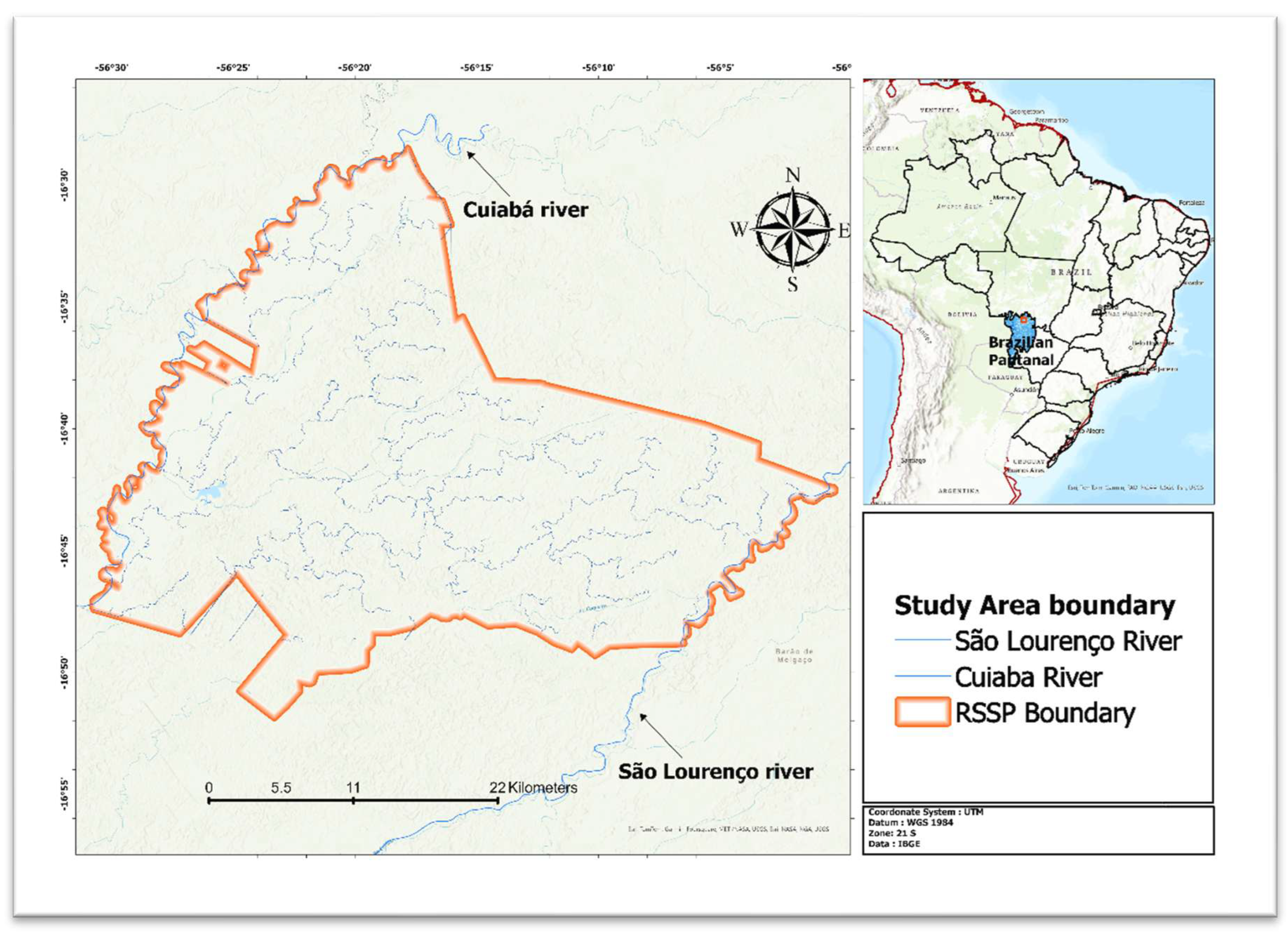
Figure 2.
Monthly average flow for Cuiabá and monthly rainfall during the period from 2017 to 2022. Data obtained from the river gauge stations at Porto Cercado on the Cuiabá River (river gauge station code: 66340000).
Figure 2.
Monthly average flow for Cuiabá and monthly rainfall during the period from 2017 to 2022. Data obtained from the river gauge stations at Porto Cercado on the Cuiabá River (river gauge station code: 66340000).
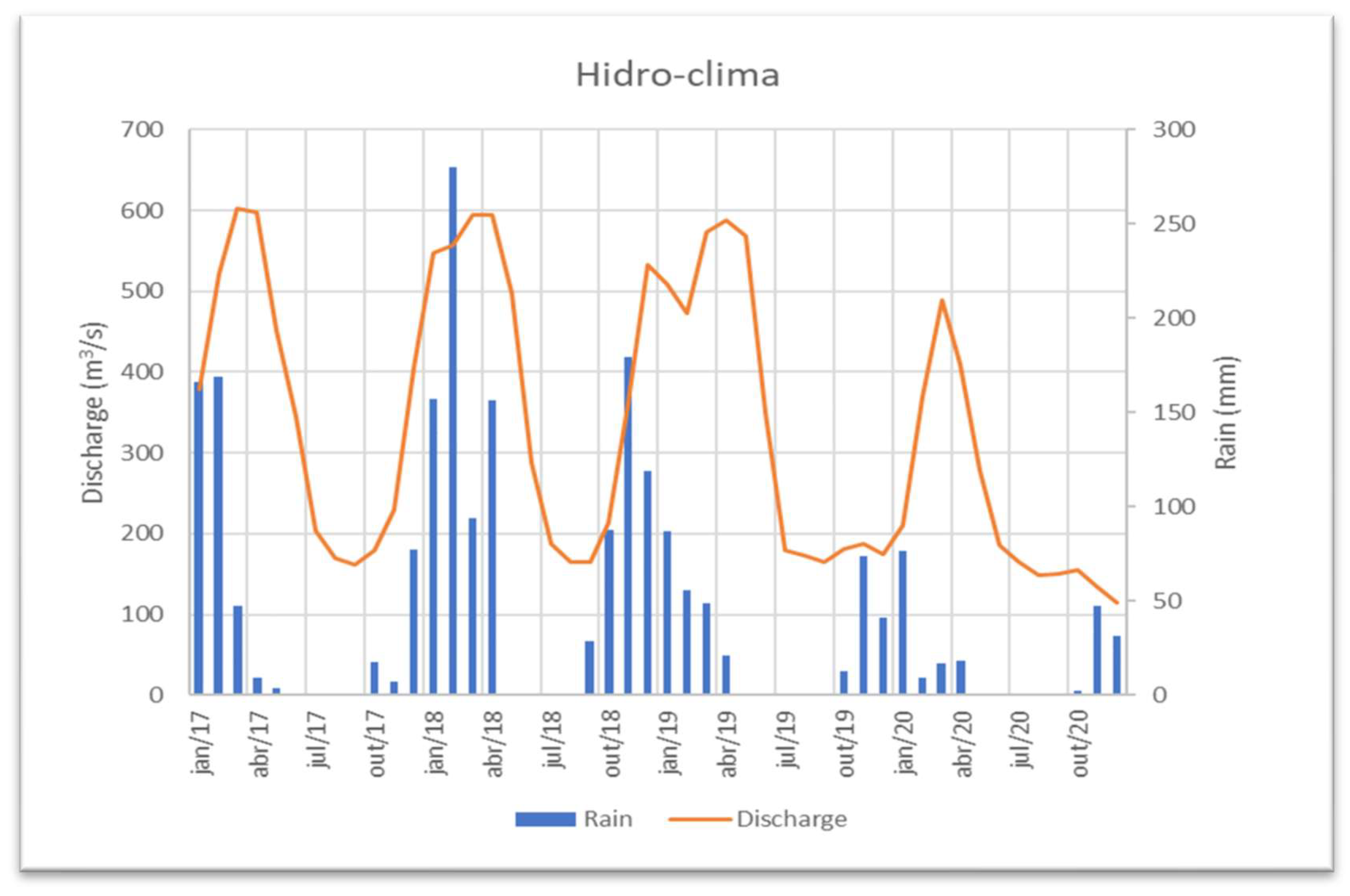
Figure 3.
Flood maps in the study area. The maps from January to April 2017 illustrate the variation of flooded areas during the flooded months. In September, at the end of the dry season, only the permanent water bodies are highlighted. Open water areas are highlighted.
Figure 3.
Flood maps in the study area. The maps from January to April 2017 illustrate the variation of flooded areas during the flooded months. In September, at the end of the dry season, only the permanent water bodies are highlighted. Open water areas are highlighted.
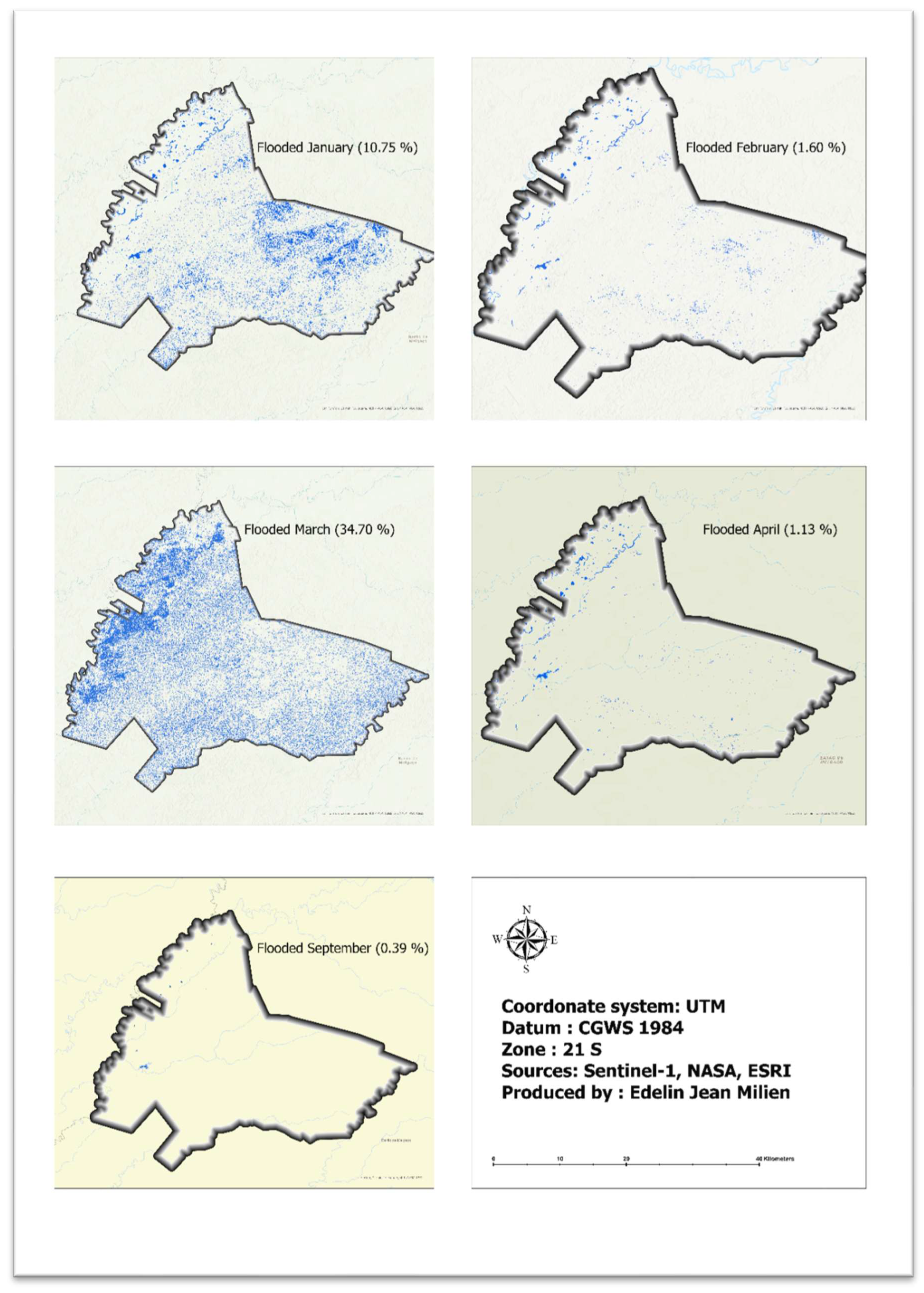
Figure 4.
Random Forest supervised classification for January, February, March and April 2017. The image was generated in the UTM coordinate system, SIRGAS 2000 Datum zone 21S.
Figure 4.
Random Forest supervised classification for January, February, March and April 2017. The image was generated in the UTM coordinate system, SIRGAS 2000 Datum zone 21S.
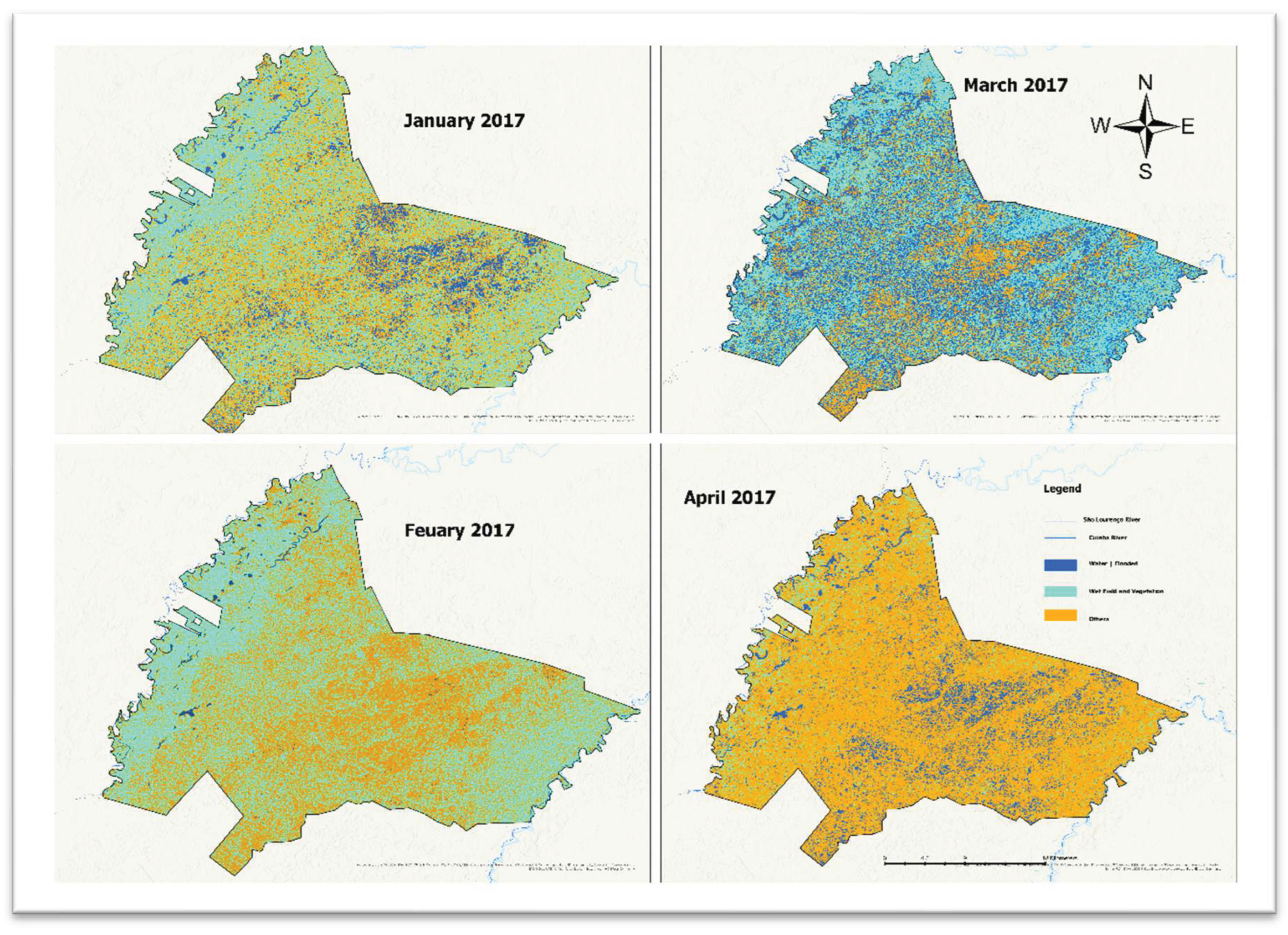

Table 1.
Temporal Variation of Flooded Areas Estimated Using the Binarization Linear Method (2017–2020).
Table 1.
Temporal Variation of Flooded Areas Estimated Using the Binarization Linear Method (2017–2020).
| Method of estimation | Flooded period | Open water bodies | Flood (ha) | Area (%) |
|---|---|---|---|
| January 2017 | 11619.6 | 10.75 | |
| February 2017 | 1731.4 | 1.60 | |
| March 2017 | 37509.8 | 34.70 | |
| Binarization linear | April 2017 | 1218.1 | 1.13 |
| September 2017 | 426.4 | 0.39 | |
| January 2020 | 1037.0 | 0.96 | |
| March 2020 | 809.3 | 0.75 | |
| September 2020 | 73.5 |
Table 2.
quantitative assessment of flooded areas derived from the random forest classification further supports the observed seasonal patterns.
Table 2.
quantitative assessment of flooded areas derived from the random forest classification further supports the observed seasonal patterns.
| Method of estimation | Period | Classes | Area (ha) | Area (%) |
|---|---|---|---|---|
| Random Forest Classification | January 2017 | Open water bodies | Flood | 11619.69 | 10.75 |
| Open Land | Vegetation | 47717.16 | 44.14 | ||
| Others | 48754.40 | 45.10 | ||
| February 2017 | Open water bodies | Flood | 831.13 | 0.77 | |
| Open Land | Vegetation | 53159.36 | 49.18 | ||
| Others | 54105.05 | 50.05 | ||
| March 2017 | Open water bodies | Flood | 37509.80 | 34.70 | |
| Open Land | Vegetation Others |
28618.17 41967.56 |
26.47 38.82 |
||
|
April 2017 |
Open water bodies | Flood Open Land | Vegetation Others |
86433.10 11587.07 10074.38 |
79.96 10.72 9.32 |
Disclaimer/Publisher’s Note: The statements, opinions and data contained in all publications are solely those of the individual author(s) and contributor(s) and not of MDPI and/or the editor(s). MDPI and/or the editor(s) disclaim responsibility for any injury to people or property resulting from any ideas, methods, instructions or products referred to in the content. |
© 2026 by the authors. Licensee MDPI, Basel, Switzerland. This article is an open access article distributed under the terms and conditions of the Creative Commons Attribution (CC BY) license (http://creativecommons.org/licenses/by/4.0/).
Copyright: This open access article is published under a Creative Commons CC BY 4.0 license, which permit the free download, distribution, and reuse, provided that the author and preprint are cited in any reuse.


