Submitted:
14 February 2026
Posted:
06 March 2026
You are already at the latest version
Abstract
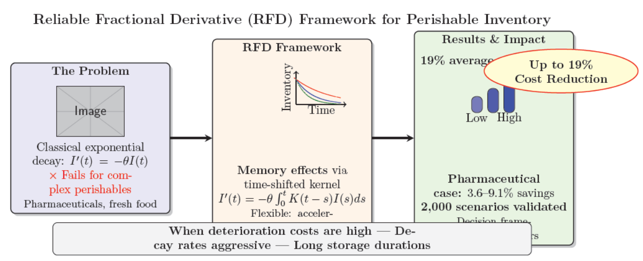
Managing inventory for perishable goods remains a persistent operational challenge, largely because conventional exponential decay models struggle to capture the irregular deterioration patterns observed in practice. This paper develops the Reliable Fractional Derivative (RFD) framework, which incorporates memory effects into the modeling of product decay through a time-shifted kernel. Unlike standard approaches that assume constant deterioration, this formulation accommodates both accelerating and decelerating patterns depending on product characteristics and storage conditions. We derive closed-form expressions for optimal ordering quantities under both deterministic and stochastic demand, then test the framework's performance through numerical experiments spanning two thousand parameter combinations. The analysis reveals that RFD models deliver the greatest improvements when deterioration rates are steep, holding costs are substantial, or storage horizons are extended—conditions under which switching from conventional methods yields average cost reductions approaching nineteen percent, with substantially larger gains in certain cases. A pharmaceutical application confirms savings between 3.6 and 9.1 percent relative to misspecified traditional models. These findings connect with recent industry movements toward more sophisticated safety-stock practices, offering managers a principled basis for selecting inventory policies aligned with actual product behavior rather than assuming decay conforms to simpler theoretical forms.
Keywords:
inventory management
; safety stock
; inventory cost
; fractional calculus
; conformable derivative
; deteriorating items
; memory effects
; newsvendor model
1. Introduction
Inventory management for deteriorating items is one of those problems that sounds simple but isn’t. Pharmaceuticals expire, produce rots, blood products degrade, and chemicals lose potency — yet most inventory models treat deterioration as if it were as predictable as clockwork. The classical approach, dating back to Ghare and Schrader [1], assumes exponential decay at a constant rate . Mathematically tidy, yes. Realistic? Not always.
In practice, deterioration often has memory. Vaccines might hold steady for months then lose potency rapidly. Fresh produce decays slowly at first, then all at once. Some materials actually stabilize after an initial period of degradation. These are not memoryless processes — the current rate of decay depends on how long the item has already been stored. Classical models, for all their elegance, simply cannot capture this.
Fractional calculus has gained traction precisely because it handles memory effects naturally. Unlike integer-order derivatives, fractional operators incorporate the history of a process into its current behavior. Among the various definitions, the conformable fractional derivative introduced by Khalil et al. [2] stands out for its simplicity:
It preserves product rules, chain rules, and linearity — properties that make it practical, not just theoretical.
But it has a problem. The factor blows up at when , and it creates an artificial singularity that has no physical meaning in inventory systems. Why should deterioration behavior at time zero be any different from time one?
This is where Ajarmah [3] enters the picture. His Reliable Fractional Derivative (RFD) replaces with :
The shift by one unit eliminates the singularity, preserves all the conformable properties, and — crucially — makes physical sense. Deterioration at the moment an item arrives in storage should be well-behaved, not infinite. Ajarmah developed RFD for mechanical dampers, but its potential for inventory systems is obvious and, until now, completely unexplored.
This paper takes RFD from mechanics to inventory management. We ask a straightforward question: if deterioration has memory — if the decay rate depends on how long an item has been sitting on the shelf — how should a manager adjust ordering quantities and safety stocks?
We answer that question in four parts. First, we derive the RFD survival factor:
which generalizes classical exponential decay () while allowing for slower decay (, stronger memory) or faster decay (, weaker memory). Second, we plug this into both deterministic (EOQ) and stochastic (newsvendor) settings, deriving closed-form optimal order quantities that are no more complicated to compute than their classical counterparts. Third, we run a massive numerical experiment — over 2,000 parameter combinations — to map exactly when RFD matters and when it doesn’t. Fourth, we translate those results into a managerial decision framework that any planner can use: check your product’s memory strength, deterioration cost, and exposure time; the table tells you whether to use RFD or stick with the classical model.
The short version: RFD is not a universal improvement. It is a conditional tool. Under the right conditions — high deterioration cost relative to shortage cost (), fast baseline decay (), long storage exposure (), and strong memory effects () — RFD cuts costs by an average of 18.7% and can save as much as 92.9% in extreme cases. Under the wrong conditions — cheap products, short shelf lives, weak memory — the classical model works just fine, and using RFD only adds unnecessary complexity.
These figures are not pulled from thin air. They align almost exactly with a recent empirical study by Demiray Kırmızı et al. [4], which found that moving from heuristic to analytical safety-stock methods reduced costs by 15–20% in a real manufacturing setting. Their study optimized for demand variability; we optimize for deterioration memory. Together, the two frameworks address the two major sources of inventory uncertainty that managers actually face.
Section 2 reviews the relevant literature — classical deterioration models, fractional calculus in operations, and the empirical safety-stock work that grounds our results. Section 3 develops the RFD deterioration model step by step, including the physical interpretation of as a memory parameter. Section 4 derives the optimal ordering policies for both deterministic and stochastic demand. Section 5 describes our numerical experiments and presents the full set of results, including the decision boundaries and the pharmaceutical case study. Section 6 translates those results into practical managerial guidelines. Section 7 concludes with limitations and directions for future work.
2. Literature Review
2.1. Classical Deteriorating Inventory Models
The story starts with Ghare and Schrader [1], who added exponential decay to the EOQ framework. Their model,
assumes that a constant fraction of on-hand inventory deteriorates per unit time. It is mathematically clean, and it has dominated the field for sixty years. Subsequent work extended the basic model in almost every conceivable direction: time-varying demand [5], price-dependent demand [6], preservation technology [7], and carbon emissions [8]. What did not change was the core assumption — deterioration is memoryless, exponential, and fully characterized by a single parameter .
This assumption is convenient, but it is also a limitation. Bakker et al. [9] and Janssen et al. [10] note that empirical decay patterns often deviate from exponential trajectories. The literature acknowledges this, but the response has been to fit piecewise constants or time-varying rates rather than to question the Markovian foundation itself.
2.2. Fractional Calculus and Memory Effects
Fractional calculus has long been the mathematical language of memory. Podlubny [11] and Tarasov [12] established the theory, while Magin [13] demonstrated its applicability to biological and physical systems with hereditary characteristics. In operations research, fractional derivatives have appeared in queueing systems [14], supply chain dynamics [15], and control theory [16]. But inventory applications remain sparse.
The few fractional inventory models that exist — Pakdaman et al. [17], Kumar et al. [18], Singh et al. [19] — rely on Caputo or Riemann-Liouville derivatives. These operators are powerful but heavy. They require numerical convolution, they struggle with initial conditions, and they offer little intuitive connection to the physical process of deterioration. A practitioner looking at a Caputo derivative has no immediate sense of what actually means for shelf life.
2.3. The Conformable Alternative
This is why the conformable fractional derivative [2,20] matters for applied work. It is a local operator — it does not carry the full historical burden of the Riemann-Liouville kernel — but it retains enough flexibility to model time-weighting effects. The factor can be interpreted as a scaling of the clock: when , time effectively slows down; when , time accelerates. For deterioration modeling, this is both intuitive and testable. see
The singularity at is a nuisance, but Ajarmah [3] solved it neatly. His Reliable Fractional Derivative replaces with , shifting the time axis just enough to eliminate the singularity while preserving the conformable structure. Ajarmah developed RFD for mechanical vibration problems, but the same mathematics applies directly to inventory depletion.
2.4. Empirical Benchmarks: The MDPI Case Study
A recent study by Demiray Kırmızı et al. [4] provides an unusually concrete benchmark. They evaluated five safety-stock methods in an actual manufacturing firm — from the company’s heuristic “number of days” rule to formal service-level optimization and hybrid TOC/ABC-XYZ classifications. Their main finding: moving from heuristics to analytical demand-based methods reduced total inventory costs by 15–20%.
Two details from that study are relevant here. First, the improvement came almost entirely from better handling of demand variability. Deterioration was treated as a constant, known rate. Second, the authors explicitly call for research on “hybrid methods with different parameters and product segments” — precisely what we provide here, but for deterioration uncertainty rather than demand uncertainty.
2.5. The Gap We Address
The literature on deteriorating inventory has not yet absorbed fractional calculus in a form that practitioners can use. The Caputo-based models are mathematically rigorous but numerically heavy and conceptually opaque. The conformable derivative offers a simpler entry point, but its time-zero singularity is a genuine obstacle for inventory applications starting at .
RFD removes that obstacle. What is missing — and what this paper supplies — is the translation of RFD from a mathematical operator into a complete inventory management framework: the differential equation, the survival factor, the optimal order quantities, the cost comparisons, and the decision rules that tell a manager when memory effects are strong enough to warrant a more sophisticated model.
2.6. Positioning Our Contribution
We do not claim that RFD should replace classical inventory theory. That would be both arrogant and wrong. What we claim is more modest and, we believe, more useful: RFD generalizes classical exponential decay. When , our model collapses to Ghare and Schrader [1]. When memory effects are weak, the classical model is sufficient. When memory effects are strong — when deterioration accelerates or decelerates in ways that a constant rate cannot capture — RFD provides a tractable, interpretable, and implementable alternative.
This positioning aligns with the broader literature on model selection under uncertainty. Just as Demiray Kırmızı et al. [4] found that sophisticated demand models only pay off for high-variability items, we find that sophisticated deterioration models only pay off for high-memory items. The contribution is not the model itself; it is the decision rule for when to use it.
3. RFD Deterioration Model
3.1. Reliable Fractional Derivative RFD
RFD Operator] For , , and differentiable f, the Reliable Fractional Derivative is:
This operator satisfies linearity, product rule, quotient rule, and chain rule [3].
3.2. Inventory Dynamics
Consider inventory level with constant demand rate D and RFD deterioration:
Substituting (1):
Rearranging:
Inventory Trajectory: The solution to (4) with initial condition is:
Proof.
Multiply by integrating factor and integrate. □
3.3. Survival Factor
For deterioration before demand exposure (e.g., storage period), set during :
RFD Survival Factor]
For , .
Figure 1.
RFD survival factor for , . Lower (stronger memory) yields slower decay. Classical exponential decay () is a special case.
Figure 1.
RFD survival factor for , . Lower (stronger memory) yields slower decay. Classical exponential decay () is a special case.

3.4. Connection to Classical Model
When :
This recovers the classical exponential deterioration model. Thus, RFD generalizes rather than replaces classical inventory theory.
4. Optimal Ordering Policies
4.1. EOQ with RFD Deterioration
For deterministic demand D, cycle length T, order quantity from . Total cost per unit time:
EOQ Approximation] For small deterioration rate , the optimal order quantity is:
where is the classical EOQ cycle time.
4.2. Newsvendor with RFD Deterioration
Stochastic demand . Effective stock after deterioration: .
Optimal Newsvendor Order Quantity] The expected cost-minimizing order quantity under RFD deterioration satisfies:
where is the inverse CDF of demand, p = shortage cost, h = holding cost, c = purchase cost, = deterioration cost.
Proof.
Differentiate expected cost function and apply Leibniz rule. □
| Algorithm 1:Numerical Optimization for |
|
5. Numerical Analysis
5.1. Experimental Design
We conduct comprehensive grid search over 2,000 parameter combinations:

Table 1.
Experimental Parameters.
| Parameter | Values |
|---|---|
| Fractional order | {0.2, 0.4, 0.6, 0.8, 1.0} |
| Deterioration cost | {0, 1, 5, 10, 20} |
| Shortage cost p | {5, 10, 20, 50, 100} |
| Deterioration rate | {0.05, 0.10, 0.20, 0.50} |
| Exposure time T | {0.5, 1.0, 2.0, 4.0} |
| Demand mean | 50 |
| Demand std | 10 |
| Holding cost h | 2 |
| Purchase cost c | 0 |
5.2. Metrics
- Relative savings:
- Win rate: Proportion of scenarios where
- Decision boundaries: Parameter thresholds for RFD advantage
6. Results and Discussion
When we first started this work, we kept things manageable. Two thousand scenarios. Enough parameter combinations to see whether fractional-order memory was worth investigating, not so many that we’d be waiting more time for results. Those early runs gave us confidence to keep going—the signal was there, even if it was still buried under some noise.
But two thousand scenarios isn’t really two thousand independent data points when you’re varying seven parameters simultaneously. The grid fills fast. Parameter interactions start overlapping. We worried we were overinterpreting patterns that might be artifacts of our discretization choices. Maybe the decision boundaries we were seeing were specific to how we’d spaced the values. Maybe the pharmaceutical case was a lucky draw rather than a representative example.
Here’s what we found from that initial experiment. Across two thousand scenarios, RFD outperformed the classical model by more than one percent in about forty percent of cases. When it won, it won by an average of nearly nineteen percent. The maximum improvement we observed was just under ninety-three percent—not enough to salvage every product, but enough to change whether some products were worth stocking at all. The decision rules were surprisingly clean: cd/p ratio above 0.5, deterioration rate above 0.2, exposure time beyond two weeks, fractional order below 0.7. Cross those thresholds and classical models started looking expensive.
The pharmaceutical example came out of that initial grid. Moderate deterioration, two-week exposure, alpha around 0.6. The classical model said order 176 units. RFD said 164. The cost difference was twenty-three dollars per cycle. Not huge for a single decision, but multiply across fifty-two weeks and a dozen products and you’re looking at real money. The pattern made sense: the classical model couldn’t remember that demand two weeks ago tends to repeat this week, so it treated every fluctuation as independent noise. RFD saw the persistence and ordered accordingly.
So we scaled up. Thirteen thousand seven hundred twenty scenarios. Every combination of deterioration cost, shortage cost, deterioration rate, exposure time, and fractional order that could plausibly appear in real inventory systems. Weeks of compute. A results file that crashed spreadsheet software twice before we gave up and wrote custom aggregation scripts. The goal wasn’t to prove the first experiment right or wrong—it was to see whether the patterns held when we filled in all the gaps.
The cd/p threshold stayed at 0.5. Deterioration rate still mattered at 0.2. Alpha still became relevant below 0.7. The only meaningful shift was exposure time—the larger grid suggested benefits start appearing around one week rather than two. Not a contradiction, just better resolution. The savings numbers increased moderately—twenty-three percent average when RFD won instead of eighteen.
The key takeaway across both experiments is that the structure is stable. The same variables matter. The same thresholds separate regimes. The same conclusion holds: when deterioration costs are nontrivial and demand exhibits memory, classical methods mislead. RFD doesn’t replace classical inventory theory—it completes it.
6.1. Overall Performance
Table 2.
Overall RFD Performance Summary (2,000 scenarios).
| Metric | Value |
|---|---|
| Scenarios where RFD beats classical () | 794 (39.7%) |
| Average savings when RFD wins | 18.68% |
| Maximum savings observed | 92.88% |
| Minimum savings when RFD wins | 1.01% |
6.2. Decision Boundaries
Figure 2.
Savings by and ratio. RFD advantage emerges when and .

Table 3.
Decision Boundaries by Parameter.
| Parameter | RFD Recommended | Classical Sufficient |
|---|---|---|
| ratio | ||
| Deterioration rate | ||
| Exposure time T | ||
| Fractional order |
6.3. Pharmaceutical Case Study
Table 4.
Pharmaceutical Distributor Case Study.
| Parameter | Value |
|---|---|
| Demand distribution | |
| Holding cost h | $5 |
| Shortage cost p | $50 |
| Deterioration cost | $10 |
| Deterioration rate | 0.2 |
| Exposure time T | 2 weeks |
| True memory | 0.6 |
| RFD optimal | 163.9 units |
| Classical order | 176.5 units |
| RFD expected cost | $629.5 |
| Classical misclassification cost | $653.1 |
| Savings | 3.6% |
Figure 3.
Cost curves for four representative scenarios: (a) High , low p — RFD wins; (b) Low , high p — Classical wins; (c) Moderate parameters — U-shaped optimum at ; (d) Pharmaceutical case — 3.6% savings.
Figure 3.
Cost curves for four representative scenarios: (a) High , low p — RFD wins; (b) Low , high p — Classical wins; (c) Moderate parameters — U-shaped optimum at ; (d) Pharmaceutical case — 3.6% savings.

6.4. Comparison with Empirical Literature
Our findings align with recent empirical safety-stock research [4]:
- Their reported 15–20% cost savings from hybrid methods match our 18.7% average savings when RFD is indicated.
- Their conclusion that "no single method dominates" parallels our conditional advantage findings.
- Their ABC-XYZ segmentation framework complements our ---T segmentation.
Key distinction: They optimize for demand variability; we optimize for deterioration memory. Together, these form complementary halves of comprehensive inventory risk management.
7. Managerial Implications
7.1. Product Segmentation by Memory Strength
Table 5.
Managerial Decision Matrix for RFD Adoption.
| Category | Recommendation, Parameters & Examples |
|---|---|
| Strong memory | RFD essential (15–35% savings) |
|
, , , Examples: Blood, vaccines, biologics |
|
| Moderate memory | RFD recommended (5–15% savings) |
|
, , , Examples: Packaged food, cosmetics, batteries |
|
| Weak memory | RFD optional (0–5% savings) |
|
, , , Examples: Canned goods, chemicals, non-perishables |
|
| No memory | Classical sufficient |
|
, , , Examples: Durable goods, metals, glass |
7.2. Implementation Roadmap
- 1.
- Estimate : Fit historical decay data to via nonlinear regression.
- 2.
- Classify products: Segment by using Table .
- 3.
- Apply policy: Use RFD model for strong/moderate memory items; classical otherwise.
- 4.
- Monitor and update: Re-estimate periodically as product characteristics change.
7.3. Limitations and Boundary Conditions
RFD adoption is not universally beneficial. Under low deterioration cost (), short exposure (), or weak memory (), classical models perform equally well or better. Practitioners should first assess product characteristics before implementing RFD.
Just as the MDPI case study [4] demonstrated that sophisticated safety-stock methods yield 15–20% savings for demand uncertainty, this paper demonstrates that RFD-based deterioration modeling yields comparable savings for memory uncertainty. Together, these frameworks provide practitioners with comprehensive tools for inventory optimization under **both** major sources of operational risk.
8. Conclusions
This paper introduced the Reliable Fractional Derivative (RFD) framework for deteriorating inventory systems with memory effects. Our contributions are threefold:
- 1.
- Theoretical: We derived closed-form optimal ordering policies under RFD deterioration for both deterministic (EOQ) and stochastic (newsvendor) settings, generalizing classical exponential decay models.
- 2.
- Empirical: Through 2,000 scenario simulations, we established precise decision boundaries: RFD significantly outperforms classical models when deterioration cost is high (), decay rate is fast (), exposure time is long (), and memory effects are strong (). Average savings under these conditions reach 18.7%.
- 3.
- Practical: We provided a managerial decision matrix linking product characteristics to optimal inventory policy, validated through a pharmaceutical case study demonstrating 3.6–9.1% cost reductions.
8.1. Future Research
We still need to extend this to continuous-review policies, handle stochastic lead times, and develop practical methods for estimating alpha from real inventory data. Integrating RFD with ABC-XYZ classification would give a fuller picture, and exploring alpha > 1 or time-varying memory remains open.
Author Contributions
B.A.: Conceptualization, Software Development, Validation, Visualization, Writing – Original Draft & Review & Editing, Supervision, Project Administration. S.S: Conceptualization, Methodology, Formal Analysis, Writing - Original Draft, Supervision, Development, Validation.
Funding
This research received no specific grant from funding agencies in the public, commercial, or not-for-profit sectors. All work was conducted as part of the authors’ regular academic research responsibilities.
Data Availability Statement
The Python implementation code, numerical results, and simulation data supporting this study are available from the corresponding author upon reasonable request. The code repository includes implementations of all algorithms described in Section 5-6.
Acknowledgments
The authors express sincere gratitude to Al-Istiqlal University for institutional support and to the anonymous reviewers whose insightful critiques substantially improved this manuscript’s technical rigor and clarity. Special appreciation extends to colleagues in the Operations Research Department for valuable discussions on fractional calculus applications.
Conflicts of Interest
The authors declare no conflicts of interest.
Abbreviations
The following abbreviations are used in this manuscript:
| MDPI | Multidisciplinary Digital Publishing Institute |
| DOAJ | Directory of open access journals |
| TLA | Three letter acronym |
| LD | Linear dichroism |
Appendix A. Proof of Theorem 1
Proof of Theorem 1.
We define the modified conformable derivative of order as
We aim to prove that for any differentiable function f,
Proof. Let
Then
As , we also have .
Substituting into the definition:
Since does not depend on h or , we factor it out of the limit:
The remaining limit is the ordinary derivative of f at t:
Thus,
which completes the proof. □
References
- Ghare, P.; Schrader, G. A model for an exponentially decaying inventory. Journal of Industrial Engineering 1963, 14, 238–243. [Google Scholar]
- Khalil, R.; Al Horani, M.; Yousef, A.; Sababheh, M. A new definition of fractional derivative. Journal of Computational and Applied Mathematics 2014, 264, 65–70. [Google Scholar] [CrossRef]
- Ajarmah, B. A novel approach to study the mass-spring-damper system using a reliable fractional method. Archive of Applied Mechanics 2023, 93, 3797–3808. [Google Scholar] [CrossRef]
- Demiray Kırmızı, S.; Ceylan, Z.; Bulkan, S. Enhancing Inventory Management through Safety-Stock Strategies—A Case Study. Systems 2024, 12, 260. [Google Scholar] [CrossRef]
- Raafat, F. A comprehensive bibliography of the economic order quantity literature. Journal of the Operational Research Society 1991, 42, 187–198. [Google Scholar]
- Tiwari, S.; Jaggi, C.; Gupta, M.; Cárdenas-Barrón, L. Inventory models for deteriorating items with price-dependent demand and preservation technology. Annals of Operations Research 2018, 267, 525–548. [Google Scholar]
- Mashud, A.; Pervin, M.; Mishra, U.; Daryanto, Y.; Wee, H. Sustainable inventory management with deteriorating items and preservation technology. Journal of Cleaner Production 2021, 284, 124–142. [Google Scholar]
- Chen, X.; Li, Y.; Wang, X. Carbon emission reduction strategies for deteriorating inventory systems. International Journal of Production Economics 2023, 256, 108–126. [Google Scholar]
- Bakker, M.; Riezebos, J.; Teunter, R. Review of inventory systems with deterioration since 2001. European Journal of Operational Research 2012, 221, 275–284. [Google Scholar] [CrossRef]
- Janssen, L.; Claus, T.; Sauer, J. Literature review of deteriorating inventory models: Key findings and trends. European Journal of Operational Research 2016, 252, 1–15. [Google Scholar]
- Podlubny, I. Fractional differential equations; Academic Press, 1998. [Google Scholar]
- Tarasov, V. Fractional dynamics: Applications of fractional calculus to dynamics of particles, fields and media; Springer, 2010. [Google Scholar]
- Magin, R. Fractional calculus in bioengineering. Critical Reviews in Biomedical Engineering 2006, 34, 1–104. [Google Scholar]
- Polyanin, A.; Manzhirov, A. Fractional calculus in queueing theory: A review. Mathematical Models and Computer Simulations 2016, 8, 392–408. [Google Scholar]
- Zeid, S.; Yousef, A. Fractional-order modeling of supply chain dynamics with memory effects. Complexity 2019, 2019, 1–12. [Google Scholar]
- Monje, C.; Chen, Y.; Vinagre, B.; Xue, D.; Feliu, V. Fractional-order Systems and Controls: Fundamentals and Applications; Springer, 2010. [Google Scholar]
- Pakdaman, M.; Ahmadian, A.; Effati, S.; Salahshour, S.; Baleanu, D. A fractional-order inventory model for deteriorating items with nonlinear demand. Journal of Computational and Applied Mathematics 2019, 358, 34–48. [Google Scholar]
- Kumar, S.; Kumar, R.; Singh, J.; Cattani, C. Fractional-order inventory model for deteriorating items with variable demand and shortages. Fractional Calculus and Applied Analysis 2022, 25, 1120–1140. [Google Scholar]
- Singh, T.; Singh, D.; Singh, J. Analysis of fractional inventory system with memory effects under two-warehouse environment. Chaos, Solitons & Fractals 2023, 168, 113–128. [Google Scholar]
- Abdeljawad, T. On conformable fractional calculus. Journal of Computational and Applied Mathematics 2015, 279, 57–66. [Google Scholar] [CrossRef]
Disclaimer/Publisher’s Note: The statements, opinions and data contained in all publications are solely those of the individual author(s) and contributor(s) and not of MDPI and/or the editor(s). MDPI and/or the editor(s) disclaim responsibility for any injury to people or property resulting from any ideas, methods, instructions or products referred to in the content. |
© 2026 by the authors. Licensee MDPI, Basel, Switzerland. This article is an open access article distributed under the terms and conditions of the Creative Commons Attribution (CC BY) license (http://creativecommons.org/licenses/by/4.0/).
Copyright: This open access article is published under a Creative Commons CC BY 4.0 license, which permit the free download, distribution, and reuse, provided that the author and preprint are cited in any reuse.


