
Submitted:
14 February 2026
Posted:
27 February 2026
You are already at the latest version
Abstract
Urban air quality is a key component of environmental sustainability and public health in large metropolitan areas. Following the substantial but temporary improvements in air quality observed during the COVID-19 lockdowns, it remains unclear whether structural changes in urban air pollution have persisted in the post-pandemic period. This study analyzes the temporal dynamics of major atmospheric pollutants in Mexico City between 2021 and 2024, including CO, NO₂, NOₓ, O₃, PM₁₀, PM₂.₅, and SO₂, using hourly data collected by the official air quality monitoring network SIMAT. Annual and monthly median concentrations were computed to reduce the influence of extreme values and short term pollution episodes. Station level monotonic trends were evaluated using the non-parametric Mann–Kendall test, complemented by Sen’s slope estimator to quantify the magnitude and direction of change. Absolute and relative changes between 2021 and 2024 were also analyzed to capture incremental variations not reflected by trend significance tests, together with hourly monthly analyses to characterize diurnal and seasonal patterns. Results indicate that no statistically significant monotonic trends were detected for any pollutant across the analyzed stations (p > 0.05), suggesting an overall stabilization of air quality levels during the post-pandemic period. Nevertheless, mod-erate increases in annual median concentrations were observed at specific locations, particularly for PM₁₀, PM₂.₅, NO₂, and NOₓ, with relative changes ranging from ap-proximately 5% to 35%. Persistent diurnal and seasonal patterns were identified, closely associated with traffic activity, photochemical processes, and meteorological conditions. These findings suggest that, although no robust long-term trends are evident, incre-mental increases and stable temporal structures remain relevant from a sustainability perspective. Continued monitoring and targeted air quality management strategies are therefore necessary to support long-term urban environmental sustainability.
Keywords:
urban air quality
; post-pandemic period
; Mann–Kendall test
; non-parametric trend analysis
; Mexico city
; ozone
; particulate matter
; environmental sustainability
1. Introduction
1.1. Global Relevance of Urban Air Quality
Air quality remains a central challenge for urban sustainability, particularly in large metropolitan areas experiencing sustained population growth, increasing traffic congestion, and intensified industrial activity. In megacities such as Mexico City, these dynamics exacerbate atmospheric emissions and pose significant challenges for public health and environmental governance. Monitoring and analyzing air quality is therefore a critical component not only for informing public policy but also for raising societal awareness and supporting preventive health strategies.
From a development perspective, urban air pollution has often been discussed within the framework of the environmental Kuznets curve, whereby pollution levels initially increase during early stages of economic development and are expected to decline as income rises and cleaner technologies are adopted [1]. However, empirical evidence suggests that this transition is neither automatic nor guaranteed, particularly in rapidly growing urban regions. Assessing whether air quality trends exhibit sustained temporal improvements is thus essential for advancing cleaner and more resilient cities.
The public health implications of air pollution are well documented. Prolonged exposure to particulate matter and gaseous pollutants has been associated with systemic inflammatory responses, respiratory diseases, childhood asthma, lung cancer, and cardiovascular conditions [2]. Moreover, air pollution has been linked to premature mortality from cardio-respiratory illnesses [3], among numerous other adverse health outcomes [4].
In the Latin American context, the ESCALA multicity study highlighted alarming associations between air pollution and mortality. In Mexico City, PM₁₀ concentrations were significantly associated with increased mortality from cardiopulmonary, respiratory, cardiovascular, cerebrovascular, and chronic obstructive pulmonary diseases, while ambient ozone (O₃) was also linked to all cause mortality, albeit with smaller effect sizes compared to particulate matter [5].
Consistent with this evidence, the World Health Organization [6] has emphasized that ambient air pollution causes millions of premature deaths annually and leads to substantial losses in healthy life years. Generating integrated, longitudinal, and well analyzed air quality information is therefore essential for supporting environmental education strategies, improving public health outcomes, and advancing sustainable urban development [2]. In this regard, air quality management directly contributes to the United Nations Sustainable Development Goals, particularly Goal 3 (Good Health and Well-Being) and Goal 11 (Sustainable Cities and Communities) [7].
1.2. COVID-19 Lockdowns and the Post-Pandemic Rebound
The COVID-19 pandemic introduced an unprecedented natural experiment for urban air quality. During periods of strict lockdown, numerous studies reported temporary reductions in atmospheric pollution, largely driven by declines in vehicular traffic and industrial activity. In particular, significant decreases in nitrogen dioxide (NO₂) were observed across many urban regions [8,9].
However, evidence regarding the persistence of these improvements remains inconclusive. Pollutants less directly linked to mobility, such as PM₂.₅, often showed limited or delayed responses to lockdown measures [8,10,11]. In the Mexican context, reductions in air pollutant concentrations during COVID-19 were lower than initially expected, suggesting structural sources of pollution beyond short-term mobility changes [12].
Additionally, secondary pollutants such as ozone (O₃) exhibited complex and sometimes counterintuitive behavior. While primary pollutants like SO₂ and NO₂ declined in many regions, O₃ concentrations remained stable or even increased in certain cities due to altered photochemical regimes [10,13]. Importantly, most studies agree that these air quality improvements were largely transient, with pollutant levels rebounding during the post-lockdown period [11].
1.3. Knowledge Gap and Research Motivation
Despite the growing body of literature on air quality during the COVID-19 pandemic, several limitations persist. Most existing studies are short-term, focus on a single pollutant, or concentrate exclusively on the year 2020. Comprehensive post-pandemic assessments that simultaneously examine multiple pollutants over extended periods remain scarce, particularly in Latin American megacities.
Mexico City, one of the largest metropolitan areas worldwide, represents a critical yet underexplored case in this regard. There is limited empirical evidence evaluating how air pollutant dynamics evolved during the post-pandemic period using recent data, station-level resolution, and robust statistical approaches. Addressing this gap is essential for distinguishing between temporary disruptions and structural changes in urban air quality.
To respond to this need, the present study conducts a multi-pollutant analysis using hourly data from 2021 to 2024 obtained from the Mexico City Atmospheric Monitoring System (SIMAT), operated by the Secretariat of the Environment of Mexico City [14]. By applying robust non-parametric methods, this research examines post-pandemic air quality dynamics and compares the behavior of primary and secondary pollutants, generating evidence relevant for urban sustainability and policy design.
1.4. Objective and Contributions
The objective of this study is to analyze the post-pandemic temporal dynamics of major atmospheric pollutants in Mexico City during the period 2021–2024. The main contributions of this work are fourfold: (i) it provides a recent multi year, multi pollutant assessment of air quality in a Latin American megacity; (ii) it applies robust non-parametric trend analysis methods suitable for non normal and heteroscedastic environmental data; (iii) it compares the temporal behavior of primary and secondary pollutants at the station level; and (iv) it offers empirical evidence to support urban sustainability strategies and air quality governance in the post pandemic context.
2. Materials and Methods
2.1. Global Studies on Temporal Air Pollution Dynamics in Large Cities
A substantial body of literature has examined temporal trends, interannual variability, and seasonal patterns of air pollutants in large urban areas worldwide. These studies consistently highlight the role of traffic intensity, urban growth, meteorological conditions, and regional characteristics in shaping air quality dynamics. In Asian megacities, particulate matter and nitrogen-based pollutants have been widely analyzed using both ground-based monitoring and modeling approaches. For instance, [15] investigated PM₂.₅ concentrations along heavily trafficked routes in Seoul, South Korea, employing the RLINE dispersion model and finding strong agreement with national monitoring networks. Long-term analyses in Iran and China further revealed pronounced diurnal and seasonal patterns in PM₁₀ concentrations, often linked to dust events, temperature, and humidity [16,17].
Multi-city and multi-pollutant studies have expanded this perspective by incorporating broader spatial scales and more diverse analytical techniques. Research conducted in several Indian megacities demonstrated strong associations between particulate matter, gaseous pollutants, and climatic factors, identifying consistent seasonal trends using correlation analysis and non-parametric methods such as the Mann–Kendall test [18]. Similarly, large-scale assessments across hundreds or thousands of Chinese cities combined satellite observations, statistical modeling, and machine learning approaches to analyze tropospheric NO₂ columns and air pollution islands, highlighting the influence of urban form, vegetation cover, and socioeconomic drivers [19,20]. These global studies demonstrate the value of long-term, multi-year analyses for understanding air pollution dynamics and supporting policy design. However, many remain focused on specific pollutants, limited geographic regions, or single methodological perspectives, constraining their applicability to post-disruption urban contexts.
2.2. Methodological Approaches and Temporal Scales
Methodologically, air quality trend studies exhibit considerable heterogeneity in terms of spatial resolution, temporal coverage, and analytical depth. Some investigations rely on station-level monitoring data to characterize pollutant behavior over extended periods, applying time series models such as ARIMA or non-parametric trend detection techniques [16,21]. Others integrate satellite derived observations with meteorological variables and machine learning algorithms, enabling broader spatial coverage and the assessment of urban scale drivers [19,22]. Despite these advances, several limitations persist. A significant proportion of studies focus on short term periods or specific interventions, such as traffic restrictions or emission control policies, while fewer examine multi-year post-intervention dynamics. Moreover, although multi pollutant analyses are increasingly common, they are often limited to two or three contaminants, reducing their ability to capture interactions between primary and secondary pollutants across different temporal scales.
2.3. Evidence from Mexico and Latin America
In Mexico and other Latin American countries, air quality research has primarily emphasized short term analyses, often motivated by specific emission sources, festive events, or the COVID-19 lockdown period. Several studies document variations in PM₂.₅, PM₁₀, and NO₂ concentrations in response to localized factors such as industrial activity, traffic intensity, or seasonal events. For example, [23] characterized particulate matter levels in Atoyac, Mexico, linking seasonal variability to sugarcane industry activity and associated health impacts. [24] analyzed short-term increases in PM₂.₅ concentrations during Christmas and New Year celebrations in Querétaro using low-cost sensors, while [25] reported reductions in NO₂ and PM₂.₅ associated with compliance with traffic speed limits. Recent methodological contributions have incorporated satellite observations and machine learning techniques to estimate pollutant concentrations in urban environments. [22], for instance, developed a random forest model combining Sentinel satellite data, meteorological variables, and ground-based observations to estimate NO₂ concentrations in Mexico City. However, these studies generally focus on single pollutants or limited temporal windows, with few addressing post-2021 dynamics in a comprehensive, multi-pollutant framework.
2.4. COVID-19 Studies and Transition to the Post-Pandemic Period
The COVID-19 pandemic provided a natural experiment to assess the sensitivity of urban air quality to abrupt changes in mobility and economic activity. Studies conducted in Mexico and other Latin American megacities consistently reported short term reductions in traffic-related pollutants such as NO₂, CO, and PM₁₀ during lockdown periods, while secondary pollutants exhibited more heterogeneous responses [26,27]. In some cases, PM₂.₅ concentrations remained stable despite mobility restrictions, underscoring the contribution of non-traffic emission sources. Importantly, existing evidence suggests that these improvements were largely temporary, with pollutant levels rebounding during the post-lockdown phase. Nevertheless, most COVID-related studies focus on the year 2020 or early 2021, leaving a critical gap in understanding how air quality has evolved during the subsequent recovery period. Comprehensive post-pandemic assessments covering multiple pollutants, extended time horizons, and station-level data in Latin American megacities remain limited.
Systematic reviews further support the notion that COVID-19 lockdowns led to widespread but temporary improvements in air quality. A recent PRISMA, based systematic review synthesizing evidence from multiple regions worldwide reported significant reductions in most ambient air pollutants, including PM₂.₅, PM₁₀, NO₂, SO₂, CO, during lockdown periods, primarily attributed to reduced industrial activity and road traffic. However, the review also highlighted controversial and region-specific responses of ozone (O₃), with increases frequently observed, particularly in East Asia, largely driven by meteorological and photochemical factors. Importantly, these findings reinforce the view that air quality improvements during the pandemic were largely transitory and do not necessarily indicate long term structural changes [28]. A summary of selected studies in presented in Table A1 in the Appendix A.
3. Materials and Methods
3.1. Study Area and Data Source
This study focuses on Mexico City, one of the largest metropolitan areas in Latin America and a region facing persistent air quality challenges. Hourly concentrations of major atmospheric pollutants—carbon monoxide (CO), nitrogen dioxide (NO₂), nitrogen oxides (NOₓ), ozone (O₃), particulate matter (PM₁₀ and PM₂.₅), and sulfur dioxide (SO₂)—were obtained for the period from January 2021 to December 2024 from the Mexico City Atmospheric Monitoring System (SIMAT), operated by the Secretariat of the Environment of Mexico City [14].
The SIMAT network provides continuous measurements through 34 fixed monitoring stations distributed across the metropolitan area and constitutes the official reference system for air quality surveillance in the city. Of these, 21 monitoring stations met the data availability criteria and were consistently operational throughout the 2021–2024 period. The nomenclature and geographic characteristics of the monitoring stations are provided in Appendix A (Table A2).
3.2. Data Preprocessing and Quality Control
Prior to analysis, the hourly database was cleaned to ensure internal consistency and to reduce the influence of anomalous records. Specifically, the preprocessing stage included: (i) removal of duplicated timestamps; (ii) exclusion of physically implausible observations (e.g., negative concentrations); and (iii) elimination of records identified as invalid when quality flags were available. No temporal imputation was performed. This decision aimed to preserve observed variability and avoid introducing artificial smoothing or bias in subsequent median aggregation and trend detection.
3.3. Data Completeness Criteria and Station Selection
To ensure comparability across years and reduce the sensitivity of summaries to missingness, analyses were restricted to station pollutant series meeting a minimum data completeness threshold. A station was included for a given pollutant if at least 70% of hourly observations were available within the corresponding aggregation period (monthly and/or annual). Stations failing to meet this criterion were excluded for that pollutant and period. This criterion was applied consistently across the entire 2021–2024 horizon.
Because particulate matter series frequently present larger data gaps in monitoring networks, PM₁₀ and PM₂.₅ analyses were limited to stations satisfying the completeness threshold across the study period. Consequently, PM₁₀ and PM₂.₅ results are interpreted cautiously as they reflect the subset of stations with consistent temporal coverage rather than the full monitoring network.
3.4. Temporal Aggregation and Descriptive Indicators
Urban air pollutant concentrations commonly exhibit skewed distributions and episodic peaks associated with short-term events (e.g., traffic surges, meteorological stagnation). Therefore, median values were used as robust summary statistics for temporal aggregation. Three aggregation levels were computed:
- Monthly medians (by month and year) to describe interannual seasonality and recovery patterns.
- Hourly monthly medians (by hour of day and month) to characterize diurnal cycles and seasonal structure.
- Annual medians (by station and year) to support trend detection and station-level comparisons.
To facilitate comparability across years, hourly monthly heatmaps were displayed using a fixed color scale based on the global concentration range observed during 2021–2024 for each pollutant. This approach prevents visual artifacts that can arise when each year is plotted with an independent scale.
3.5. Absolute and Relative Change Metrics
To complement trend testing and capture incremental variations over the study horizon, absolute and relative changes between 2021 and 2024 were computed at the station level based on annual medians:
Absolute change:
Relative change (%):
where denotes the annual median concentration in year . These indicators provide an interpretable measure of change even when formal trend tests are underpowered due to short time series. Absolute change is Delta_abs and relative change is Delta_pct in Tables 1 to 8.
3.6. Trend Detection Using Mann–Kendall and Sen’s Slope
Long-term monotonic trends were assessed at the station level using the non-parametric Mann–Kendall test applied to annual median concentrations for each pollutant over the 2021–2024 period. The Mann–Kendall test was selected because it does not assume normality, is robust to outliers, and is widely used in environmental time series analysis [29,30].
To quantify the magnitude and direction of monotonic change, Sen’s slope estimator was computed alongside the Mann–Kendall statistic. Sen’s slope provides a robust estimate of the median rate of change and is commonly used in conjunction with the Mann–Kendall test for environmental applications [30,31]. Detailed formulations of both methods are available in the cited literature.
Statistical significance was evaluated at the 5% level (α = 0.05). Given the short temporal span of the analysis (four annual observations), results were interpreted primarily in terms of: (i) statistical significance at α = 0.05; (ii) the sign and magnitude of Sen’s slope estimates; and (iii) consistency with absolute and relative change metrics, as well as with the observed seasonal and diurnal concentration patterns.
3.7. Reporting Conventions and Interpretation
Results are reported through (i) monthly median evolution plots, (ii) hourly monthly median heatmaps, and (iii) station-level tables summarizing annual medians, change metrics, and trend statistics. Because the study period is limited to four years, the trend analysis is intended to detect strong monotonic signals and to characterize post-pandemic stability versus incremental shifts, rather than to establish causal effects. Accordingly, findings are discussed in relation to urban sustainability and air quality governance implications under a post-pandemic recovery context.
4. Results
This section presents the post-pandemic temporal dynamics of major atmospheric pollutants in Mexico City during the 2021–2024 period. Results are reported separately for each pollutant to highlight differences between primary and secondary emissions, combining descriptive temporal patterns (monthly and hourly monthly medians), station-level absolute and relative changes, and non-parametric trend detection using the Mann–Kendall test and Sen’s slope estimator.
4.1. CO Results
Figure 1 shows the monthly evolution of median CO concentrations in Mexico City from 2021 to 2024. A consistent seasonal pattern is observed across all years, with higher concentrations during winter months (January–February and November–December) and lower levels during late spring and early summer (May–June). Interannual differences suggest a gradual rebound in CO levels after 2021, particularly evident in late 2023, while 2024 exhibits higher variability during mid-year months.
For comparability across years, hourly monthly heatmaps were displayed using a fixed color scale based on the global concentration range observed during 2021–2024.
Figure 2 shows the hourly monthly median CO concentration patterns for 2021 and 2024 using a common color scale. In both years, a pronounced morning peak between 7:00 and 9:00 is observed, consistent with traffic related emissions. Compared to 2021, 2024 exhibits higher peak intensities during winter months and increased variability in late summer and early autumn, suggesting a post pandemic rebound in vehicular activity.
Table 1 summarizes the absolute and relative changes in annual median CO concentrations between 2021 and 2024 at the station level. While some stations such as LPR exhibited stable concentrations over the study period, others showed substantial increases. Notably, CCA and FAC experienced relative increases of 36% and 29% (delta-pct)respectively, despite having moderate baseline concentrations in 2021.
Given the skewed distribution and episodic peaks characteristic of urban CO concentrations, median values were used as robust summary statistics for hourly, monthly, and annual aggregation. Trend detection was subsequently performed using the non-parametric Mann–Kendall test applied to annual median concentrations.
Station-level Mann–Kendall tests did not detect statistically significant monotonic trends at the 5% significance level for the 2021–2024 period in Table 2. However, all stations exhibited positive Sen’s slope estimates, indicating a consistent upward tendency in annual median CO concentrations. In several stations (e.g., CCA, CUA, and UIZ), p-values below 0.10 suggest a marginally increasing trend, which is consistent with the observed absolute and relative increases reported in Table 1.
Overall, the results indicate a stable and recurring seasonal and hourly structure in CO concentration with higher concentrations during winter and morning peak hours, a general upward tendency in CO levels from 2021 to 2024, and notable spatial heterogeneity in station level changes. While formal trend detection is limited by the short temporal span, the combined evidence from descriptive statistics, spatial patterns, and Sen’s slope estimates suggests a post 2021 increase in CO concentrations in Mexico City.
4.2. NO2 Results
Figure 3 illustrates the monthly evolution of median NO₂ concentrations in Mexico City from 2021 to 2024. A pronounced seasonal pattern is observed across all years, with higher concentrations during winter months and lower levels during summer, reflecting the combined effects of traffic related emissions and enhanced photochemical activity during warmer periods. Compared to 2021, subsequent years exhibit higher NO₂ levels, particularly during winter months, indicating a gradual rebound in urban activity. Interannual variability is more pronounced for NO₂ than for CO, consistent with the stronger sensitivity of NO₂ to short-term emission changes and atmospheric conditions.
Figure 4 shows the hourly monthly median NO₂ concentration patterns for 2021 and 2024 using a common color scale. In both years, pronounced morning peaks between 7:00 and 10:00 are observed across most months, followed by lower concentrations during midday hours, consistent with photochemical NO₂ depletion under high solar radiation. Compared to 2021, 2024 exhibits higher morning peak intensities and increased persistence of NO₂ concentrations, particularly during winter months, suggesting enhanced traffic related emissions and post pandemic recovery of urban activity.
Table 3 reports the absolute and relative changes in annual median NO₂ concentrations at the station level between 2021 and 2024. While some stations (e.g., MON and SAC) exhibited stable concentrations over the study period, most locations showed moderate increases. The largest relative increases were observed at MER and FAC (≈15%), indicating a sustained rise in traffic related NO₂ emissions. The magnitude of changes is smaller than that observed for CO, but more spatially consistent, reflecting the strong linkage between NO₂ and vehicular activity
Station-level Mann–Kendall tests applied to annual median NO₂ concentrations did not detect statistically significant monotonic trends at the 5% significance level over the 2021–2024 period, which is expected given the short length of the time series. Nevertheless, all monitoring stations exhibited positive Sen’s slope estimates, indicating a consistent upward tendency in NO₂ concentrations across Mexico City. Several stations, such as CCA and FAC, showed relatively larger slopes and absolute increases, suggesting localized intensification of traffic-related emissions.
4.3. O3 Results
Figure 5 shows the monthly evolution of median O₃ concentrations in Mexico City from 2021 to 2024. In contrast to primary pollutants, O₃ exhibits a pronounced spring maximum, with peak concentrations occurring between March and May across all years. This pattern reflects enhanced photochemical activity driven by increased solar radiation and the availability of precursor pollutants. Compared to 2021, subsequent years show progressively higher springtime O₃ levels, with 2024 displaying the highest peak values. The temporal behavior of O₃ differs markedly from that of CO and NO₂, underscoring the secondary nature of ozone formation and its nonlinear response to emission change.
Figure 6 shows the hourly monthly median O₃ concentration patterns for 2021 and 2024 using a common color scale. O₃ displays a pronounced diurnal cycle, with minimum concentrations during nighttime and early morning hours and maximum levels during midday to early afternoon (approximately 12:00–16:00), consistent with photochemical formation under high solar radiation. Seasonally, the highest O₃ concentrations occur during spring months (March–May). Compared to 2021, 2024 exhibits higher and more persistent daytime O₃ levels during the spring peak period, suggesting intensified photochemical activity and increased precursor availability and/or favorable meteorological conditions.
Table 4 summarizes station-level Mann–Kendall trend statistics together with absolute and relative changes in annual median O₃ concentrations between 2021 and 2024. Although no statistically significant monotonic trends were detected at the 5% level due to the short time series, all stations exhibited positive Sen’s slope estimates and substantial absolute and relative increases, particularly at CUT and SAC, where relative changes exceeded 50% O₃ exhibits a strong spring maximum, a pronounced daytime peak aligned with photochemical formation, and evidence of increasing levels after 2021, with 2024 showing the most intense springtime values. The temporal behavior of O₃ differs markedly from CO and NO₂, reinforcing the secondary nature of ozone formation and its nonlinear response to precursor availability and meteorological conditions.
4.4. PM10 Results
Figure 7 presents the monthly evolution of median PM₁₀ concentrations in Mexico City for the period 2021–2024, based on stations meeting the minimum data completeness criteria. PM₁₀ exhibits a clear seasonal pattern, with higher concentrations during winter and early spring and lower levels during the summer months, consistent with the combined effects of resuspension processes, atmospheric stability, and precipitation. Interannual comparisons indicate higher PM₁₀ levels in 2024 across most months relative to previous years, particularly during spring and autumn. Although the analysis is limited to five stations due to data availability constraints, the observed patterns are consistent across locations, suggesting a generalized increase in PM₁₀ levels after 2021.
The hourly monthly heatmaps of PM10 reveal a consistent diurnal cycle, with higher concentrations during morning hours and lower levels overnight, alongside a clear seasonal pattern characterized by higher values in the first half of the year. These patterns are consistent across the available monitoring stations and reflect the influence of local emission sources and meteorological conditions. Due to data completeness constraints, PM10 analyses were limited to five stations with sufficient temporal coverage.
Figure 8.
Hourly monthly median PM10 concentration patterns, a)2021, b)2024.
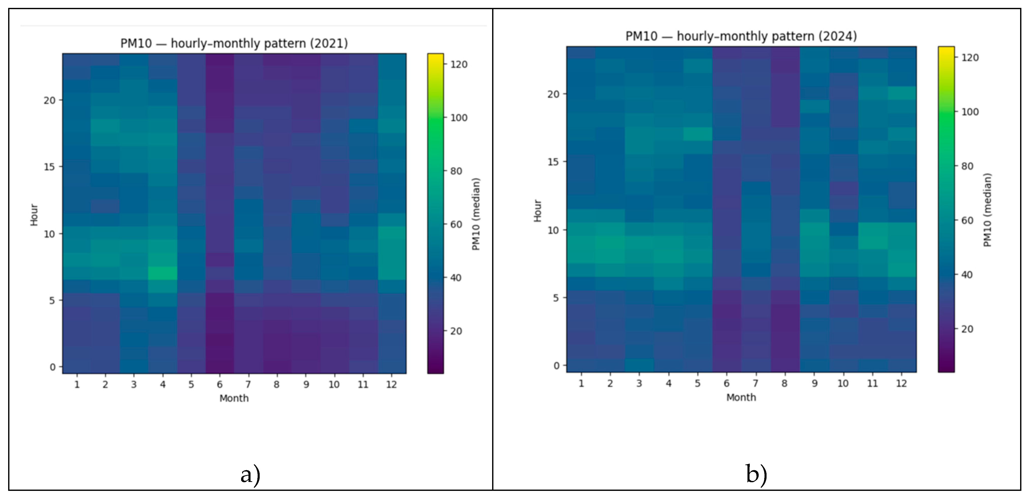
Table 5 reports the Mann–Kendall trend test and Sen’s slope estimates for annual median PM10 concentrations at stations with sufficient data coverage (n = 5). No statistically significant monotonic trends were detected between 2021 and 2024 (p > 0.05 for all stations). While some sites, such as BJU and UIZ, exhibited moderate absolute increases over the study period, these changes were not consistent enough to yield significant trends. This result suggests that PM10 levels during the study period were dominated by short term variability and seasonal dynamics rather than sustained interannual changes.
4.5. PM2.5 Results
The PM2.5 analysis was limited to five monitoring stations with sufficient data availability over the 2021–2024 period. Monthly median concentrations exhibit a clear seasonal pattern, with higher levels during the spring months and lower values in mid-year, consistent with regional meteorological conditions (Figure 9).
The results of the trend analysis for PM2.5 indicate that no statistically significant monotonic trends were detected at any of the analyzed stations during the 2021–2024 period, according to the Mann–Kendall test (p > 0.05 in all cases). Nevertheless, the analysis of absolute and relative changes reveals moderate increases in annual median PM2.5 concentrations at several stations.
In particular, stations such as BJU, CCA, FAR, and UIZ exhibited absolute increases of approximately 2 µg/m³, corresponding to relative increases of about 10–13% compared to 2021 levels, whereas MER maintained nearly constant concentrations throughout the study period. Although small, the positive Sen’s slope estimates suggest a slight upward signal that is not yet sufficient to be characterized as a statistically significant trend within the analyzed time horizon.

Table 6.
Sation-level Mann–Kendall tests, PM2.5.
| Station | trend | p | z | sen_slope | intercept | Delta_abs | Delta_pct |
|---|---|---|---|---|---|---|---|
| BJU | no trend | 0.148562 | 1.444630 | 0.583333 | 17.125 | 2.0 | 11.764706 |
| CCA | no trend | 0.371093 | 0.894427 | 0.333333 | 15.500 | 2.0 | 12.500000 |
| FAR | no trend | 1.000000 | 0.000000 | 0.333333 | 17.000 | 2.0 | 11.111111 |
| MER | no trend | 1.000000 | 0.000000 | 0.000000 | 20.000 | 0.0 | 0.000000 |
| UIZ | no trend | 1.000000 | 0.000000 | 0.333333 | 19.000 | 2.0 | 10.000000 |
These results indicate that, while no robust long-term trend is observed, incremental changes in PM₂.₅ are present and may reflect interannual variability and the influence of local and seasonal factors rather than a sustained structural change in air quality.
4.6. SO2 Results
Sulfur dioxide (SO₂) concentrations remained consistently low throughout the 2021–2024 period, with very limited temporal variability across the monitoring stations. Due to the low dynamic range of the observed values, no statistically significant monotonic trends were identified using the Mann–Kendall test. The observed month fluctuations reflect discrete changes around detection-level concentrations rather than meaningful long-term variability. SO₂ exhibited stable conditions over the study period, suggesting a limited contribution of stationary combustion sources within the urban monitoring network and reinforcing the dominance of other pollutants in shaping recent air quality dynamics in Mexico City.
The trend analysis for sulfur dioxide (SO₂) indicates no statistically significant monotonic trends at any of the analyzed stations during the 2021–2024 period, according to the Mann–Kendall test (Table 7). Sen’s slope estimates were close to zero, further supporting the absence of sustained long-term changes.
Although some stations exhibit relatively large absolute and relative changes between 2021 and 2024, these variations are driven by the very low concentration levels and the limited dynamic range of SO₂ measurements, often fluctuating around detection level values. Consequently, percentage changes should be interpreted with caution, as they do not reflect meaningful environmental shifts. Overall, SO₂ concentrations remained low and stable throughout the study period, suggesting a limited influence of stationary combustion sources within the urban monitoring network and reinforcing the secondary role of SO₂ in recent air quality dynamics in Mexico City.
4.7. NOx Results
Nitrogen oxides (NOₓ) exhibited a clear seasonal pattern, with higher median concentrations during winter months and lower values in mid-year, consistent with traffic related emission dynamics. However, the Mann–Kendall test did not identify statistically significant monotonic trends at any monitoring station during the 2021–2024 period.
Figure 10.
Monthly evolution, Nox.
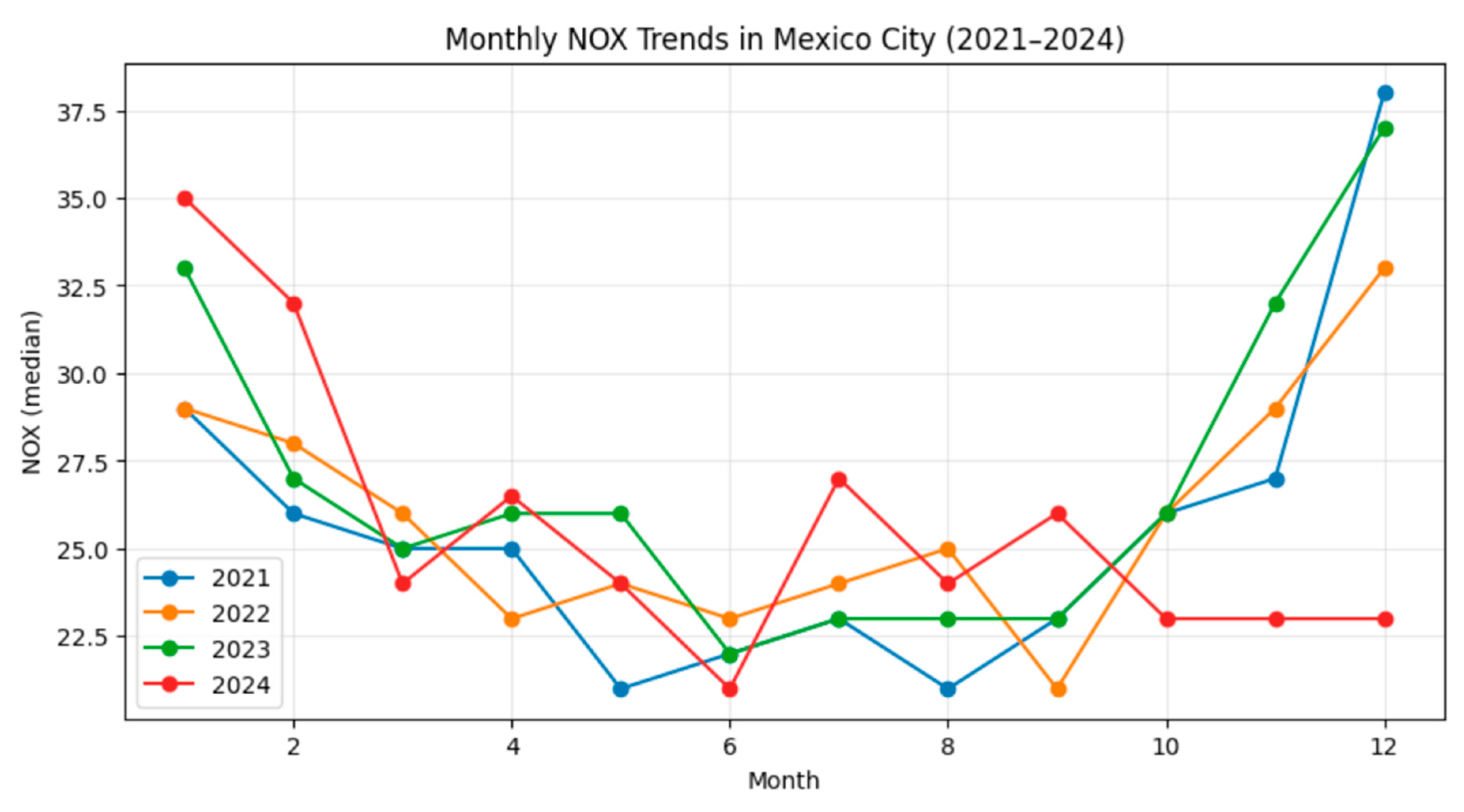
Sen’s slope estimates were generally small and heterogeneous across stations, indicating the absence of a sustained long-term increase or decrease. The observed absolute and relative changes between 2021 and 2024 reflect interannual variability rather than structural shifts in NOₓ emissions. The stability of NOₓ concentrations reinforces the findings obtained for NO₂ and supports the interpretation that primary traffic related emissions remained relatively stable in Mexico City during the post-pandemic period.
Table 8.
Sation-level Mann–Kendall tests, SO2.
| Station | trend | p | z | sen_slope | intercept | Delta_abs | Delta_pct |
|---|---|---|---|---|---|---|---|
| MGH | no trend | 0.245278 | 1.161895 | 0.416667 | 30.875 | 1.0 | 3.225806 |
| MER | no trend | 0.308180 | 1.019049 | 1.416667 | 37.375 | 4.0 | 10.810811 |
| SAG | no trend | 0.308180 | 1.019049 | 0.833333 | 24.250 | 2.0 | 8.333333 |
| CCA | no trend | 0.371093 | 0.894427 | 0.333333 | 21.500 | 2.0 | 10.000000 |
| FAC | no trend | 0.470101 | 0.722315 | 0.666667 | 26.000 | 1.0 | 3.703704 |
| CUT | no trend | 0.734095 | -0.339683 | -0.666667 | 22.500 | -1.0 | -4.761905 |
| MON | no trend | 1.000000 | 0.000000 | 0.000000 | 15.000 | 0.0 | 0.000000 |
| SAC | no trend | 1.000000 | 0.000000 | -0.166667 | 22.750 | -1.0 | -4.347826 |
Table 9 presents a summary of post pandemic pollutant behavior, trend signal refers to the qualitative indication of temporal change inferred from the combined evidence of Sen’s slope direction and magnitude, absolute and relative changes between 2021 and 2024, and the consistency of seasonal and diurnal patterns, even in the absence of statistically significant monotonic trends at α = 0.05.
5. Discussion
This study provides a comprehensive multi-pollutant assessment of air quality dynamics in Mexico City during the 2021–2024 post-pandemic period. Across all analyzed pollutants (CO, NO₂, NOₓ, O₃, PM₁₀, PM₂.₅, and SO₂), the Mann–Kendall test did not identify statistically significant monotonic trends at the station level. This result indicates an overall stabilization of air pollutant concentrations rather than pronounced long-term improvements or deteriorations following the COVID-19 mobility disruptions. The absence of significant monotonic trends should not be interpreted as an absence of change. Instead, the observed behavior suggests that air quality in Mexico City has entered a post-pandemic steady state, characterized by interannual variability and seasonal dynamics rather than structural shifts in emissions.
Primary pollutants directly linked to combustion processes, such as CO, NO₂, and NOₓ, exhibited consistent seasonal patterns dominated by traffic activity, with higher concentrations during winter months and lower levels during mid-year. Despite moderate absolute and relative increases at some stations, the absence of statistically significant monotonic trends suggests that post-pandemic mobility recovery did not translate into sustained structural emission changes.
In contrast to primary pollutants, ozone (O₃) exhibited greater variability and more pronounced seasonal dynamics, with elevated concentrations during spring and early summer months. This behavior reflects the complex photochemical formation of O₃, which depends not only on precursor availability but also on meteorological conditions such as solar radiation and temperature. Although no statistically significant monotonic trends were detected, the persistence of high O₃ levels during photochemically active periods highlights the nonlinear response of secondary pollutants to stable precursor emissions. This finding underscores the challenge of controlling ozone pollution through traffic emission reductions alone and emphasizes the importance of integrated precursor management strategies.
For PM₁₀ and PM₂.₅, the analysis was limited to stations with sufficient data coverage. Results indicate moderate increases in annual median concentrations at several stations, particularly for PM₂.₅, with relative changes on the order of 10–15% between 2021 and 2024. However, these increases were not statistically significant according to the Mann–Kendall test, and Sen’s slope estimates remained small. This suggests that particulate matter concentrations are influenced primarily by interannual variability, local conditions, and seasonal factors, rather than by sustained emission growth. The limited spatial coverage for PM₂.₅ and PM₁₀ highlights persistent challenges in long term particulate monitoring and suggests that caution is warranted when extrapolating city wide conclusions for these pollutants.
SO₂ concentrations remained consistently low throughout the study period, with minimal variability and a very limited dynamic range. The absence of statistically significant trends, combined with near-zero Sen’s slope estimates, indicates that stationary combustion sources currently play a minor role in shaping urban air quality dynamics in Mexico City. Observed relative changes in SO₂ should be interpreted cautiously, as they are largely driven by fluctuations around detection-level concentrations rather than meaningful environmental changes.
6. Conclusions
This study provides a recent (2021–2024) multi-pollutant assessment of post-pandemic air quality dynamics in Mexico City using robust non-parametric methods. The combined evidence from absolute and relative changes, Sen’s slope estimates, and temporal patterns indicates that several pollutants exhibited moderate to strong increases during the study period, particularly CO, NO₂, and O₃, as summarized in Table 9.
Primary pollutants (CO, NO₂, and NOₓ) displayed stable and recurring seasonal patterns dominated by traffic related emissions, consistent with previous findings in large metropolitan areas [15,32] In contrast, the secondary pollutant ozone (O₃) exhibited pronounced springtime maxima and a clear post-2021 increase, reflecting its nonlinear photochemical formation and sensitivity to meteorological conditions.
Although no statistically significant monotonic trends were detected due to the short temporal horizon, the presence of consistent upward signals across multiple pollutants suggests that current air quality management strategies have been insufficient to achieve sustained improvements. While Mexico City has avoided severe post-pandemic deterioration, the absence of clear long-term reductions indicates a need to strengthen integrated mitigation approaches.
In line with [4] effective urban air quality strategies should combine city renaturalization, the promotion of sustainable mobility, and data-driven management tools, including real time monitoring and advanced spatial interpolation techniques, supported by environmental education initiatives from early stages.
6.1. Limitations and Future Research
This study is subject to several limitations. First, the relatively short temporal horizon (four years) limits the statistical power of trend detection methods. Second, data availability constraints, particularly for particulate matter, reduced spatial coverage in some analyses. Finally, meteorological variables were not explicitly modeled and should be incorporated in future work to disentangle emission-driven changes from atmospheric effects.
Future research should extend the temporal scope, integrate meteorological normalization, and explore nonlinear interactions among pollutants to better inform long term air quality management strategies.
Author Contributions
Conceptualization, E.S.H.-G.; methodology, E.S.H.-G.; software, E.S.H.-G.; validation, D.C.G., (C.A.M.-I.); formal analysis, E.S.H.-G.; investigation, E.S.H.-G.; data curation, E.S.H.-G.; writing—original draft preparation, E.S.H.-G.; writing—review and editing methodology, D.C.G., (C.A.M.-I.); visualization, E.S.H.-G.; supervision, D.C.G. All authors have read and agreed to the published version of the manuscript.
Funding
This research was supported by the Secretaría de Educación, Ciencia, Tecnología e Innovacion (SECTEI) of Mexico City through the Innovation Project “Mapping and quantification of CH₄, CO, CO₂, NOx, and SO2 in soi and air in Mexico City as a mitigation strategy for reducing climate change effects SECTEI/083/2024.”.
Data Availability Statement
The data can be requested from the corresponding author when necessary, the datasets and the scripts used to perform the statistical and spatial analyses are in supplementary material.
Acknowledgments
The Mexico City Atmospheric Monitoring Directorate (SIMAT), administered by the Secretariat of the Environment of Mexico City (SEDEMA) under the General Directorate of Air Quality, is gratefully acknowledged for providing the data used in this study.
Conflicts of Interest
The authors declare no conflicts of interest.
Appendix A
Table A1.
Summary of selected studies on temporal air pollution analysis.
| Author(s) | City / Region | Period | Pollutants | Data Source | Methods | Main Focus |
|---|---|---|---|---|---|---|
| Lee & Batterman [15] | Seoul, South Korea | 2023–2024 | PM₂.₅ | Ground monitoring, traffic routes | RLINE dispersion model | Traffic-related PM₂.₅ exposure |
| Kumar et al. [33] | 7 cities, India | 2018–2021 | BC, PM₁₀, PM₂.₅, NOx, CO, SO₂ | Monitoring stations | Correlation analysis | Black carbon relationships |
| Sherrif et al. [34] | Chennai & Bengaluru, India | 2019–2023 | NO₂ | Satellite data | Statistical modeling | Spatio-temporal NO₂ patterns |
| Hamidi et al. [16] | Ahvaz, Iran | 2008–2019 | PM₁₀ | Monitoring stations | Descriptive & temporal analysis | Dust events and PM₁₀ |
| Gulia et al. [18] | 4 megacities, India | 2018–2022 | PM₁₀, PM₂.₅, NOx, SO₂, O₃ | Monitoring stations | Pearson correlation, Mann–Kendall | Seasonal variability |
| Chang et al. [19] | 346 cities, China | 2019–2023 | Tropospheric NO₂ | Satellite data | Random forest, SHAP | Urban drivers of NO₂ |
| Xiong et al. [17] | Chengdu, China | 2015–2021 | PM₁₀, PM₂.₅, O₃, NO₂ | Monitoring stations | Socio-environmental analysis | Urban growth effects |
| Singh et al. [35] | Handwar City, India | 2023–2024 | PM₂.₅, PM₁₀, NO₂, SO₂ | Monitoring stations | PCA, clustering, AQI | Critical pollution zones |
| Wen et al. [32] | SE China | 2015–2060 | PM₂.₅, PM₁₀ | Monitoring & scenarios | Forecasting, BAU scenarios | Electric vehicle adoption |
| Nasar-u-Minallah et al. [21] | Lahore, Pakistan | 2014–2024 | NOx, O₃, SO₂, PM₁₀, CO | Monitoring stations | ARIMA models | Long-term forecasting |
| Niu et al. [20] | >2000 cities, China | 2000–2020 | PM₂.₅, PM₁₀ | Monitoring & urban data | Durbin model | Air pollution island |
| Hernández-Sánchez et al. [23] | Atoyac, Mexico | – | PM₁₀, PM₂.₅ | Monitoring stations | Seasonal analysis | Industry and health |
| Monzón-Herrera et al. [22] | Mexico City | 2024 | NO₂ | Satellite & ground data | Random forest | NO₂ estimation |
| Rodríguez-Trejo et al. [25] | Querétaro, Mexico | 2023 | PM₂.₅ | Low-cost sensors | Descriptive analysis | Holiday pollution |
| Texcaloc-Sangrador et al. (2024) | Mexico | 2014–2018 | NO₂, PM₂.₅ | Traffic & monitoring data | Regression analysis | Speed limits |
| Nieto-Garzón & Lozano [25] | Mexico City, São Paulo, Bogotá | 2019–2021 | NO₂, O₃, CO, PM₁₀ | Monitoring data | Comparative analysis | COVID mobility effects |
| Méndez-Astudillo & Caetano [26] | Mexico City, Monterrey, Guadalajara | 2020 | PM₁₀, PM₂.₅ | Monitoring stations | Chow test, Mann–Whitney | Lockdown impacts |
| Martínez-Morales et al. [27] | Monterrey, Mexico | 2020–2021 | PM₂.₅ metals | Monitoring stations | Chemical analysis | Pandemic composition |
Table A2.
Nomenclature associated with air quality monitoring stations.
| Key | Name | Municipality | State | Latitude | Longitude |
|---|---|---|---|---|---|
| AJU | Ajusco | Tlalpan | CDMX | 19.1542 | -99.1626 |
| AJM | Ajusco Medio | Tlalpan | CDMX | 19.2721 | -99.2077 |
| ATI | Atizapán | Atizapán de Zaragoza | Estado de México | 19.5769 | -99.2541 |
| BJU | Benito Juarez | Benito Juárez | CDMX | 19.3716 | -99.1590 |
| CAM | Camarones | Azcapotzalco | CDMX | 19.4684 | -99.1697 |
| CHO | Chalco | Chalco | Estado de México | 9.487227 | -99.1142 |
| CUA | Cuajimalpa | Cuajimalpa de Morelos | CDMX | 19.365 | -99.2917 |
| CUT | Cuautitlán | Cuautitlán Izcalli | Estado de México | 19.6467 | 99.2102 |
| FAC | FES Acatlán | Naucalpan de Juárez | Estado de México | 19.4824 | -99.2435 |
| GAM | Gustavo A. Madero | Gustavo A. Madero | CDMX | 19.4827 | -99.0946 |
| HGM | Hospital General de México | Cuauhtémoc | CDMX | 19.41161 | -99.1522 |
| INN | Investigaciones Nucleares | Ocoyoacac | Estado de México | 19.2919 | -99.3805 |
| IZT | Iztacalco | Iztacalco | CDMX | 19.3844 | -99.1176 |
| MGH | Miguel Hidalgo | Miguel Hidalgo | CDMX | 19.4246 | -99.1195 |
| MPA | Milpa Alta | Milpa Alta | CDMX | 19.2007 | 99.0113 |
| PED | Pedregal | Álvaro Obregón | CDMX | 19.3251 | -99.2041 |
| SAG | San Agustín | Ecatepec de Morelos | Estado de México | 19.5329 | -99.0303 |
| TLA | Tlalnepantla | Tlalnepantla de Baz | Estado de México | 19.5290 | -99.2045 |
| TLI | Tultitlán | Tultitlán | Estado de México | 19.6025 | -99.1771 |
| UIZ | UAM Iztapalapa | Iztapalapa | CDMX | 19.3607 | -99.0738 |
| VIF | Villa de las Flores | Coacalco de Berriozábal | Estado de México | 19.6582 | -99.0965 |
References
- Dogan, A.; Pata, U.K. The role of ICT, R&D spending and renewable energy consumption on environmental quality: Testing the LCC hypothesis for G7 countries. J. Clean. Prod. 2022, 380, 135038. [Google Scholar] [CrossRef]
- Tavares, M.S.; Rodrigues, C.T.; de Menezes, S.L.S.; Moreno, A.M. Health at risk: Air pollution and urban vulnerability. Green Health 2025, 1, 21. [Google Scholar] [CrossRef]
- Jindal, S.K.; Aggarwal, A.N.; Jindal, A. Household air pollution in India and respiratory diseases. Curr. Opin. Pulm. Med. 2020, 26, 128–134. [Google Scholar] [CrossRef]
- Arriazu-Ramos, A.; Santamaría, J.M.; Monge-Barrio, A.; Bes-Rastrollo, M.; Gutierrez Gabriel, S.; Benito Frias, N.; Sánchez-Ostiz, A. Health impacts of urban environmental parameters: A review of air pollution, heat, noise, green spaces and mobility. Sustainability 2025, 17, 4336. [Google Scholar] [CrossRef]
- Romieu, I.; Gouveia, N.; A Cifuentes, L.; de Leon, A.P.; Junger, W.; Vera, J.; Strappa, V.; Hurtado-Díaz, M.; Miranda-Soberanis, V.; Rojas-Bracho, L.; et al. Multicity study of air pollution and mortality in Latin America (the ESCALA study). Res. Rep. Health Eff. Inst. 2012, 171, 5–86. [Google Scholar]
- World Health Organization. WHO Global Air Quality Guidelines: Particulate Matter (PM2.5 and PM10), Ozone, Nitrogen Dioxide, Sulfur Dioxide and Carbon Monoxide. Available online: https://www.who.int/publications/i/item/9789240034228 (accessed on 29 January 2025).
- United Nations. Transforming Our World: The 2030 Agenda for Sustainable Development. Available online: https://sdgs.un.org/2030agenda (accessed on 29 January 2025).
- Shi, Z.; Song, C.; Liu, B.; Lu, G.; Xu, J.; Van Vu, T.; Harrison, R.M. Abrupt changes in surface air quality attributable to COVID-19 lockdowns. Sci. Adv. 2021. [Google Scholar] [CrossRef]
- Tyagi, P.; Braun, D.; Sabath, B.; Henneman, L.; Dominici, F. Short-term change in air pollution following the COVID-19 emergency. medRxiv 2020, 2020.08.04.20168237. [Google Scholar]
- Adam, M.G.; Tran, P.T.; Balasubramanian, R. Air quality changes in cities during the COVID-19 lockdown: A critical review. Atmos. Res. 2021, 264, 105823. [Google Scholar] [CrossRef]
- Yadav, S.; Dhankhar, R.; Chhikara, S.K. Significant changes in urban air quality during COVID-19 lockdown in Rohtak City. Asian J. Chem. 2022, 34, 3189–3196. [Google Scholar] [CrossRef]
- Retana-Olvera, J.L.; Ruiz-Serrano, M. Movilidad urbana y calidad del aire en la zona metropolitana de Toluca a inicios del COVID-19. CienciAmérica 2021, 10, 81–98. [Google Scholar] [CrossRef]
- Zhang, Z.; Arshad, A.; Zhang, C.; Hussain, S.; Li, W. Temporary reduction in global air pollution during COVID-19 confinement. Remote Sens. 2020, 12, 2420. [Google Scholar] [CrossRef]
- Secretariat of the Environment of Mexico City (SEDEMA). Mexico City Atmospheric Monitoring System (SIMAT). Available online: https://www.aire.cdmx.gob.mx (accessed on 29 January 2025).
- Lee, S.J.; Batterman, S. Estimation of vehicle PM2.5 emissions with high spatio-temporal resolution and its application to air dispersion modeling in Seoul, South Korea. Environ. Pollut. 2025, 127479. [Google Scholar] [CrossRef]
- Hamidi, M.; Ghobadi, T.; Shao, Y.; Fallah, B.; Rostami, M.; Mao, R. Investigation of the role of southwestern Asia dust events on urban air pollution: A case study of Ahvaz. Sci. Rep. 2025, 15, 21981. [Google Scholar] [CrossRef] [PubMed]
- Xiong, X.; Qiu, J.; Zhao, R.; Du, P.; Zhao, L. Spatiotemporal heterogeneities of air pollution in Chengdu. Front. Environ. Sci. 2025, 13, 1540671. [Google Scholar] [CrossRef]
- Gulia, S.; Kumar, K.; Kumar, P.; Yadav, A.; Rajni. Navigating urban air pollution: Trends and climate links in Indian megacities. Environ. Qual. Manag. 2025, 35, e70210. [Google Scholar] [CrossRef]
- Cheng, F.; Sun, Q.; Zhang, J.; Liu, J.; Lü, W.; Shen, F.; Yang, H. Nitrogen dioxide pollution in 346 Chinese cities: Spatiotemporal variations and natural drivers frommulti-source remote sensing data. PLoS ONE 2025, 20, e0334535. [Google Scholar] [CrossRef]
- Niu, L.; Zhang, Z.; Liang, Y.; van Vliet, J. Spatiotemporal patterns of the urban air pollution island effect. Environ. Int. 2024, 184, 108455. [Google Scholar] [CrossRef]
- Nasar-u-Minallah, M.; Jabbar, M.; Zia, S.; Perveen, N. Assessing environmental challenges in Lahore. Environ. Monit. Assess. 2024, 196, 865. [Google Scholar] [CrossRef]
- Monzón Herrera, Y.R.; Polanco Gaytán, M.; Aquino Santos, R.T.; Babu Saheer, L.; Mendoza-Cano, O.; Macedo-Barragán, R.J. Estimating surface NO₂ in Mexico City using Sentinel-5P and machine learning. Atmosphere 2025, 17, 37. [Google Scholar] [CrossRef]
- Hernandez-Sánchez, U.A.; Meléndez-Armenta, R.Á.; González-Moreno, H.R.; López-Méndez, M.C.; Rico-Barragán, A.A. Impacts of sugarcane industry on air quality and public health in Atoyac, México. Urban Clim. 2025, 64, 102700. [Google Scholar] [CrossRef]
- Rodríguez-Trejo, A.; Böhnel, H.N.; Ibarra-Ortega, H.E.; Salcedo, D.; González-Guzmán, R.; Castañeda-Miranda, A.G.; Chaparro, M.A. Air quality monitoring with low-cost sensors in Querétaro. Atmosphere 2024, 15, 879. [Google Scholar] [CrossRef]
- Texcalac-Sangrador, J.L.; Pérez-Ferrer, C.; Quintero, C.; Galbarro, F.J.P.; Yamada, G.; Gouveia, N.; Barrientos-Gutierrez, T. Speed limits and their effect on air pollution in Mexico City. Sci. Total Environ. 2024, 924, 171506. [Google Scholar] [CrossRef] [PubMed]
- Nieto-Garzón, O.; Lozano, A. Different local air-pollution responses to COVID-19 lockdown measures. Air Qual. Atmos. Health 2025, 1–16. [Google Scholar]
- Méndez-Astudillo, J.; Caetano, E. The effect of abrupt changes to sources of PM10 and PM2.5 concentrations in Mexico. Atmosphere 2023, 14, 596. [Google Scholar] [CrossRef]
- SeyedAlinaghi, S.; Karimi, A.; Pashaei, A.; Kianzad, S.; Soleymanzadeh, M.; Mojdeganlou, H.; Afsahi, A.M. The effects of the COVID-19 pandemic on air pollution: A systematic review. Coronaviruses 2025, 6, E030724231565. [Google Scholar] [CrossRef]
- Thenmozhi, M.; Kottiswaran, S.V. Analysis of rainfall trend using Mann–Kendall test and Sen’s slope estimator. Int. J. Agric. Sci. Res. 2016, 6, 131–138. [Google Scholar]
- Venegas, Q.; Thomasson, M.; García, P. Trend analysis using Mann–Kendall and Sen’s slope estimator. Am. J. Environ. Sci. 2020, 15, 180–187. [Google Scholar] [CrossRef]
- Sen, P.K. Estimates of the regression coefficient based on Kendall’s tau. J. Am. Stat. Assoc. 1968, 63, 1379–1389. [Google Scholar] [CrossRef]
- Wen, Z.N.; Miao, Q.Y.; Chen, J.R.; Wu, S.P.; He, L.X.; Jiang, B.Q.; Huang, Z. Heavy metal emissions from on-road vehicles in southeastern China. Environ. Sci. Pollut. Res. 2025, 32, 298–313. [Google Scholar] [CrossRef]
- Kumar, V.; Devara, P.C.; Soni, V.K. Spatiotemporal variations in black carbon aerosol concentration in India. MAUSAM 2026, 77, 219–234. [Google Scholar] [CrossRef]
- Sheriff, R.; Meer, M.S.; Tariq, A. Remote sensing-based assessment of vegetation and LST effects on NO₂ concentrations. Eng. Rep. 2026, 8, e70436. [Google Scholar]
- Singh, J.; Kumar, P.; Kale, A.; Yadav, A.K.; Maurya, P.K.; Kumar, D.; Ahamad, F. Spatio-temporal analysis of air quality in Haridwar City. Environ. Monit. Assess. 2025, 197, 889. [Google Scholar] [CrossRef] [PubMed]
Figure 1.
Montly evolution, CO.
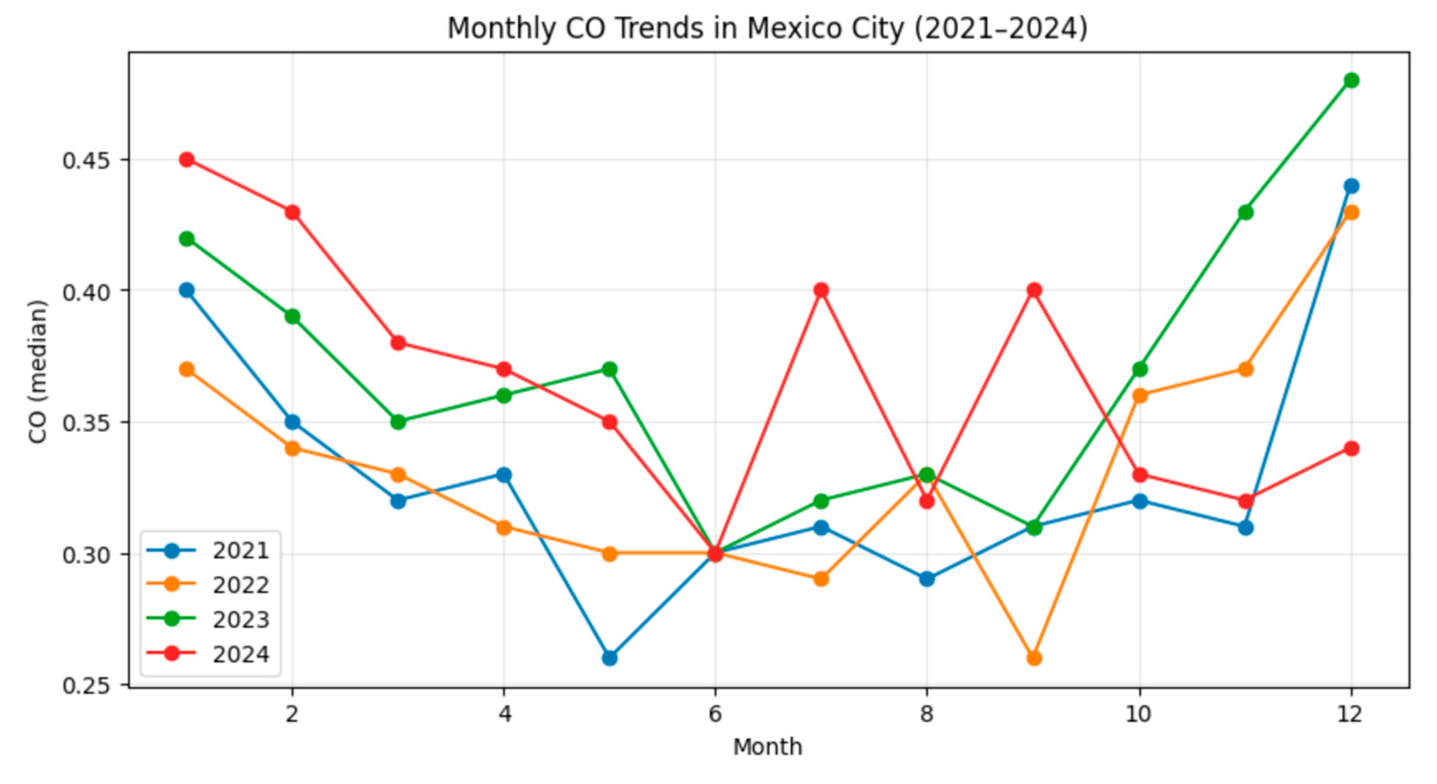
Figure 2.
Hourly–monthly median CO concentration patterns, a)2021, b)2024.
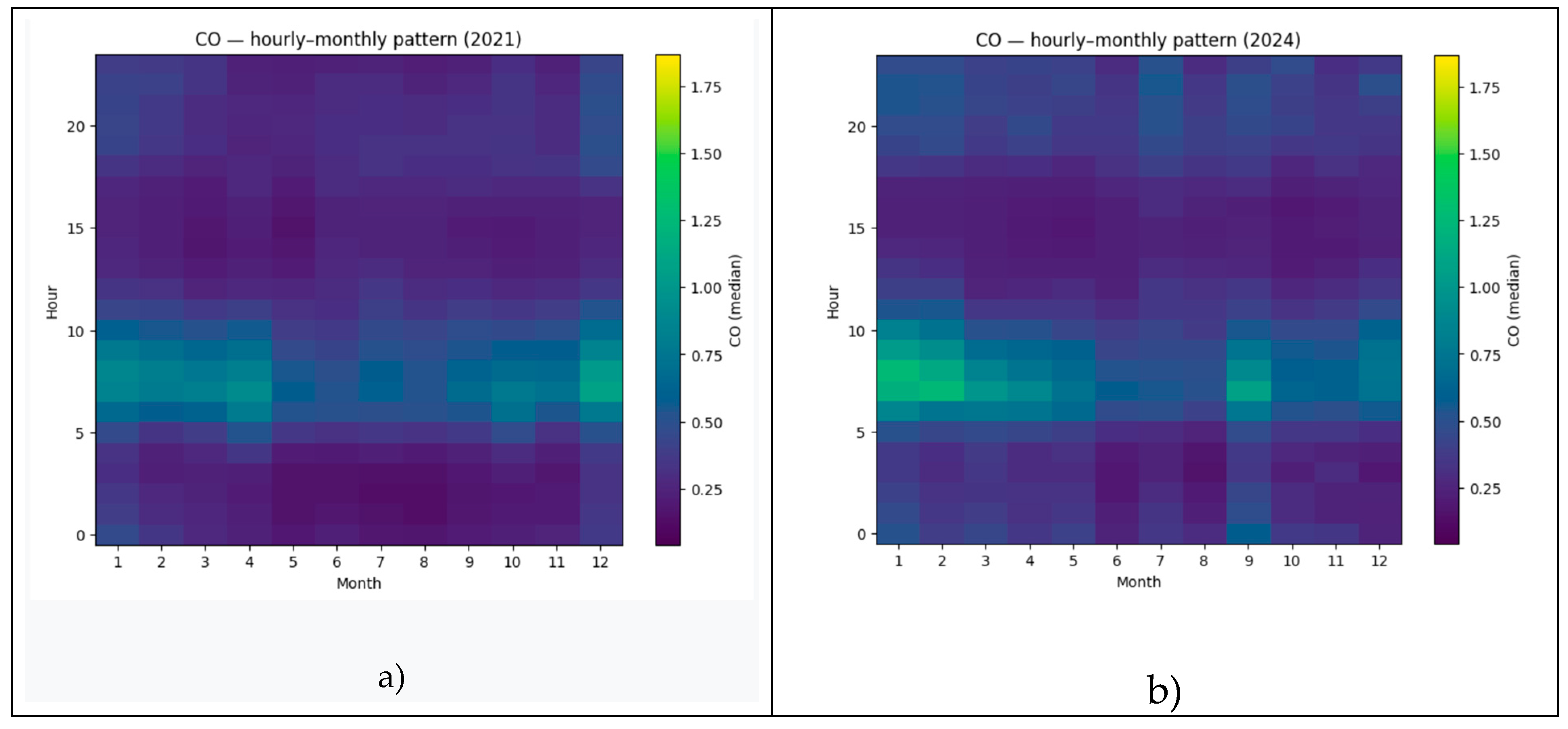
Figure 3.
Monthly evolution, NO2.
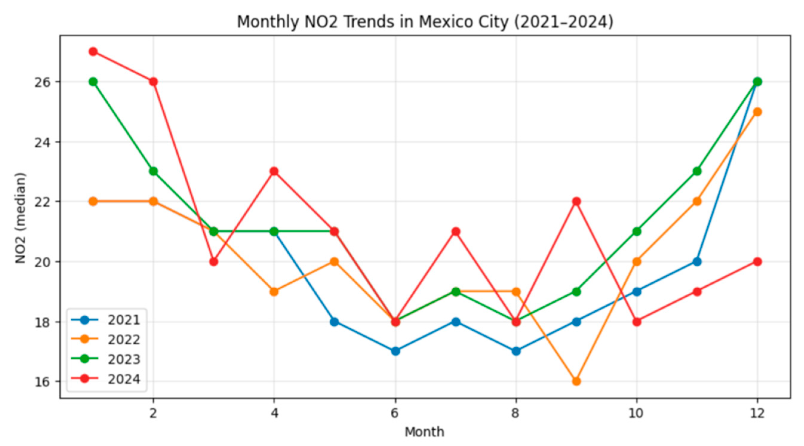
Figure 4.
Hourly monthly median NO2 concentration patterns, a)2021, b)2024.
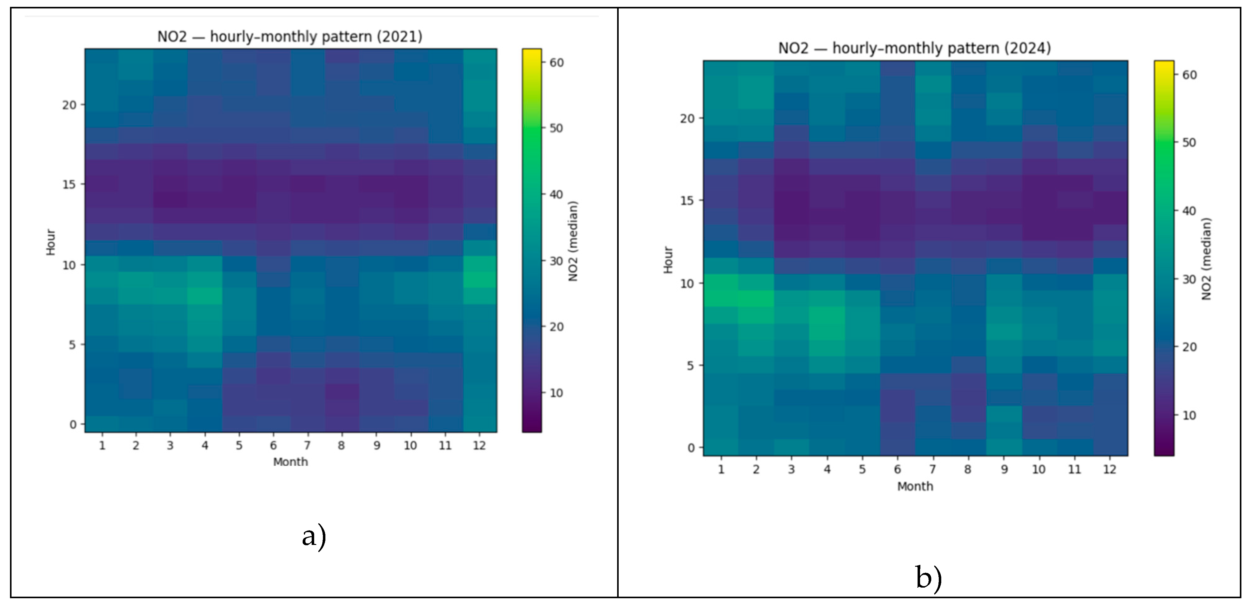
Figure 5.
Monthly evolution, O3.
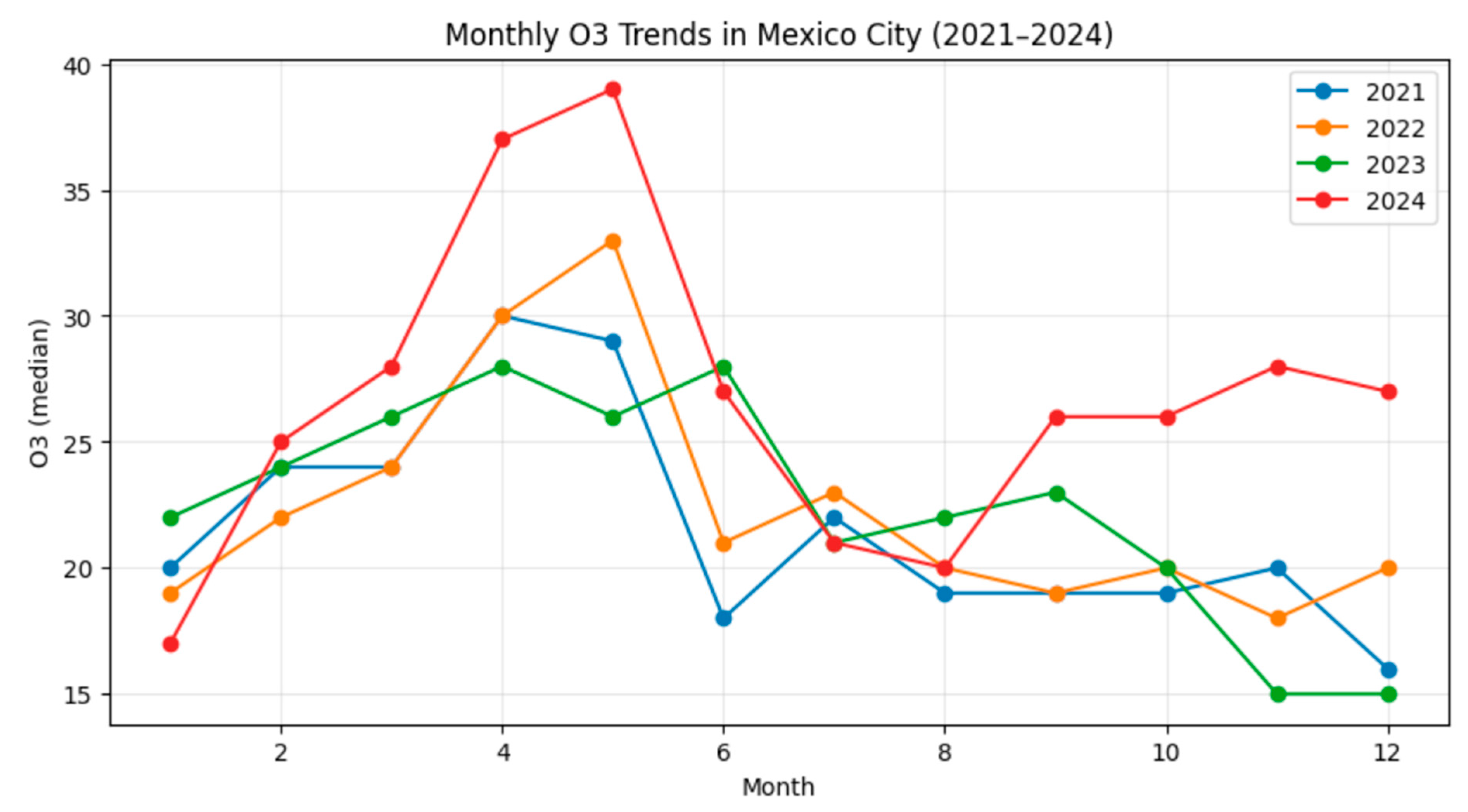
Figure 6.
Hourly–monthly median NO2 concentration patterns, a)2021, b)2024.
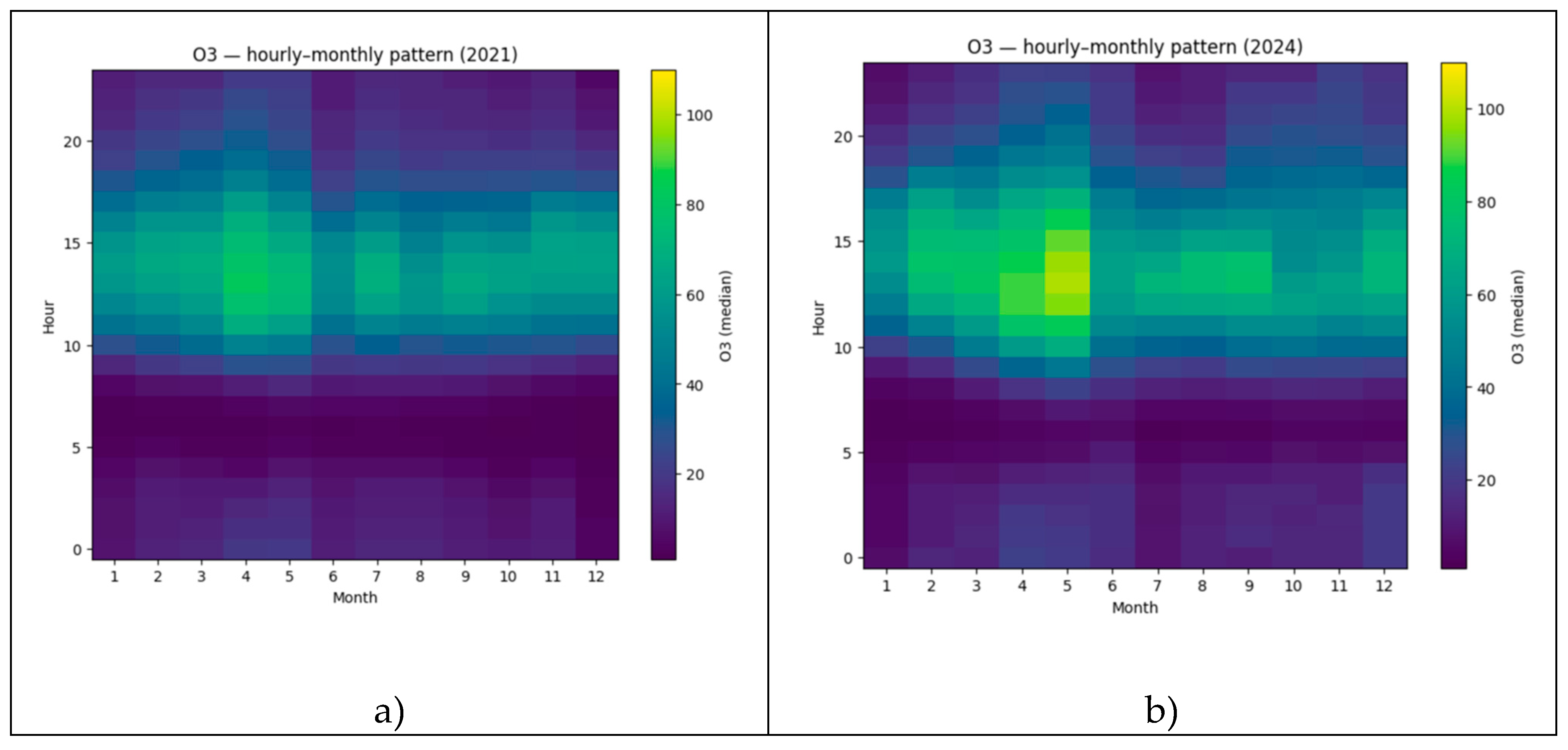
Figure 7.
Monthly evolution, PM10.
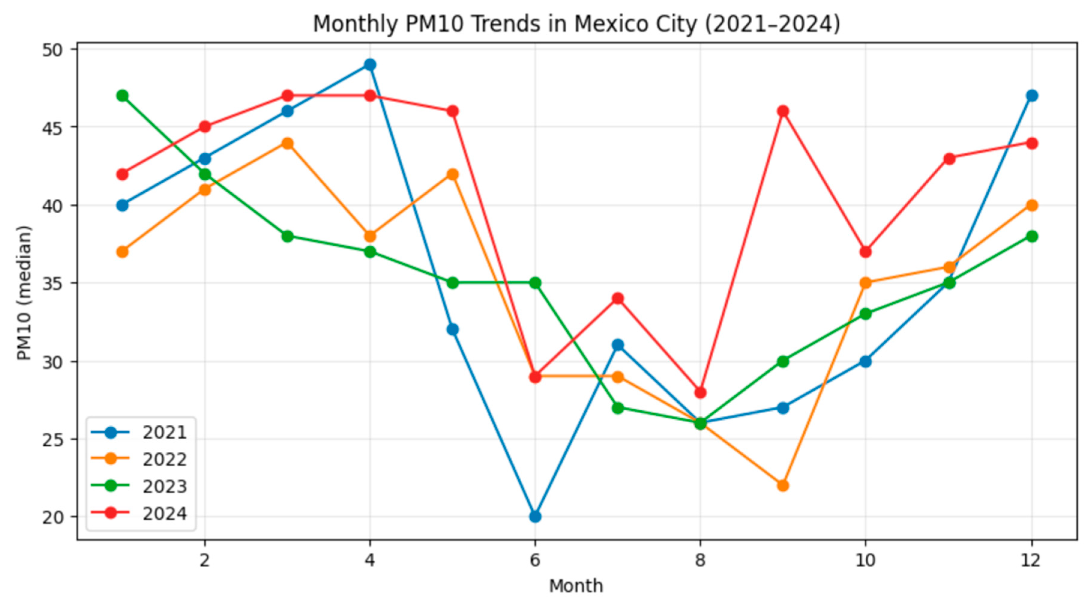
Figure 9.
Monthly evolution, PM2.5.
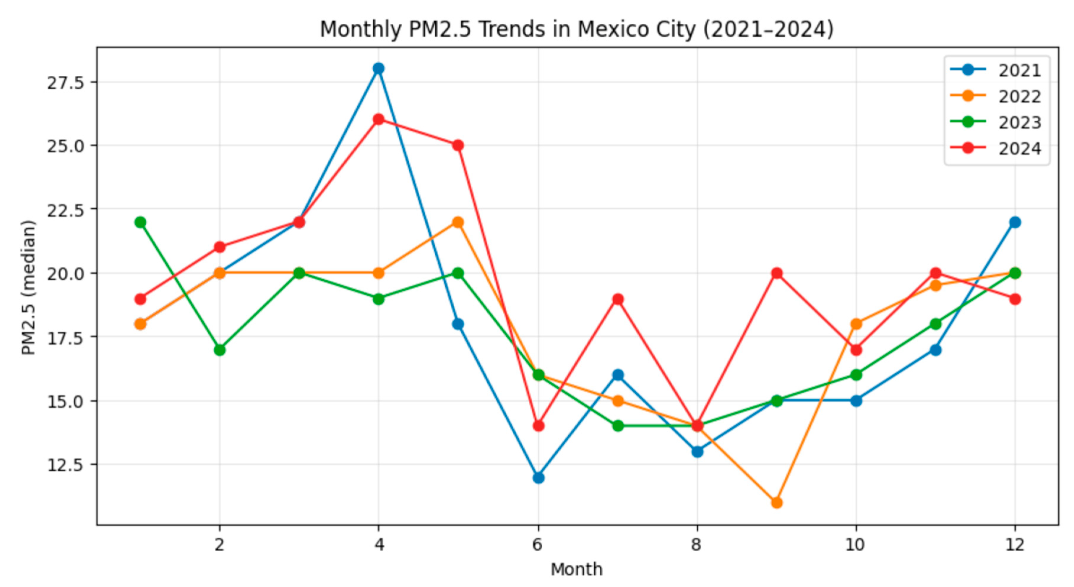
Table 1.
Annual median CO concentrations.
| Estacion | 2021 | 2022 | 2023 | 2024 | Delta_abs | Delta_pct |
|---|---|---|---|---|---|---|
| LPR | 0.46 | 0.49 | 0.51 | 0.46 | 0.00 | 0.000000 |
| SAC | 0.35 | 0.33 | 0.37 | 0.36 | 0.01 | 2.857143 |
| MGH | 0.34 | 0.33 | 0.36 | 0.36 | 0.02 | 5.882353 |
| BJU | 0.31 | 0.32 | 0.35 | 0.34 | 0.03 | 9.677419 |
| FAR | 0.28 | 0.27 | 0.30 | 0.32 | 0.04 | 14.285714 |
| MER | 0.39 | 0.39 | 0.45 | 0.45 | 0.06 | 15.384615 |
| UIZ | 0.33 | 0.33 | 0.37 | 0.39 | 0.06 | 18.181818 |
| CUA | 0.25 | 0.27 | 0.31 | 0.31 | 0.06 | 24.000000 |
| FAC | 0.31 | 0.30 | 0.36 | 0.40 | 0.09 | 29.032258 |
| CCA | 0.25 | 0.28 | 0.32 | 0.34 | 0.09 | 36.000000 |
Table 2.
Sation-level Mann–Kendall tests, CO.
| Station | trend | p | z | sen_slope | intercept | Delta_abs | Delta_pct |
|---|---|---|---|---|---|---|---|
| CCA | no trend | 0.089429 | 1.698416 | 0.030000 | 0.2550 | 0.09 | 36.000000 |
| CUA | no trend | 0.148562 | 1.444630 | 0.020000 | 0.2600 | 0.06 | 24.000000 |
| UIZ | no trend | 0.148562 | 1.444630 | 0.020000 | 0.3200 | 0.06 | 18.181818 |
| MER | no trend | 0.245278 | 1.161895 | 0.025000 | 0.3825 | 0.06 | 15.384615 |
| FAC | no trend | 0.308180 | 1.019049 | 0.035000 | 0.2825 | 0.09 | 29.032258 |
| FAR | no trend | 0.308180 | 1.019049 | 0.016667 | 0.2650 | 0.04 | 14.285714 |
| BJU | no trend | 0.308180 | 1.019049 | 0.010000 | 0.3150 | 0.03 | 9.677419 |
| MGH | no trend | 0.470101 | 0.722315 | 0.008333 | 0.3375 | 0.02 | 5.882353 |
| SAC | no trend | 0.734095 | 0.339683 | 0.006667 | 0.3450 | 0.01 | 2.857143 |
| LPR | no trend | 1.000000 | 0.000000 | 0.010000 | 0.4600 | 0.00 | 0.000000 |
Table 3.
Sation-level Mann–Kendall tests, NO₂.
| Station | trend | p | z | sen_slope | intercept | Delta_abs | Delta_pct |
| MER | no trend | 0.089429 | 1.698416 | 1.416667 | 26.875 | 4.0 | 14.814815 |
| FAC | no trend | 0.148562 | 1.444630 | 1.000000 | 19.000 | 3.0 | 15.000000 |
| MGH | no trend | 0.148562 | 1.444630 | 0.833333 | 23.250 | 2.0 | 8.333333 |
| SAG | no trend | 0.245278 | 1.161895 | 0.833333 | 19.750 | 2.0 | 10.000000 |
| CCA | no trend | 0.371093 | 0.894427 | 0.166667 | 18.750 | 1.0 | 5.555556 |
| FAR | no trend | 0.470101 | 0.722315 | 0.833333 | 16.750 | 2.0 | 11.111111 |
| BJU | no trend | 0.470101 | 0.722315 | 0.666667 | 21.000 | 1.0 | 4.761905 |
| CUT | no trend | 1.000000 | 0.000000 | 0.166667 | 17.250 | 1.0 | 6.250000 |
| MON | no trend | 1.000000 | 0.000000 | 0.000000 | 13.000 | 0.0 | 0.000000 |
| SAC | no trend | 1.000000 | 0.000000 | 0.000000 | 19.000 | 0.0 | 0.000000 |
Table 4.
Sation-level Mann–Kendall tests, O3.
| Station | trend | p | z | sen_slope | intercept | Delta_abs | Delta_pct |
|---|---|---|---|---|---|---|---|
| CUT | no trend | 0.089429 | 1.698416 | 2.666667 | 16.000 | 10.0 | 55.555556 |
| MON | no trend | 0.089429 | 1.698416 | 2.000000 | 25.000 | 6.0 | 24.000000 |
| SAC | no trend | 0.089429 | 1.698416 | 3.583333 | 21.125 | 11.0 | 50.000000 |
| SAG | no trend | 0.089429 | 1.698416 | 1.333333 | 18.500 | 5.0 | 29.411765 |
| UIZ | no trend | 0.089429 | 1.698416 | 1.500000 | 20.250 | 6.0 | 28.571429 |
| PED | no trend | 0.148562 | 1.444630 | 2.000000 | 23.000 | 9.0 | 36.000000 |
| TLA | no trend | 0.148562 | 1.444630 | 1.333333 | 17.000 | 5.0 | 27.777778 |
| MGH | no trend | 0.308180 | 1.019049 | 1.666667 | 19.000 | 4.0 | 19.047619 |
| BJU | no trend | 0.470101 | 0.722315 | 1.833333 | 19.750 | 8.0 | 36.363636 |
| NEZ | no trend | 0.470101 | 0.722315 | 2.166667 | 20.750 | 7.0 | 30.434783 |
Table 5.
Sation-level Mann–Kendall tests, PM10.
| Station | trend | p | z | sen_slope | intercept | Delta_abs | Delta_pct |
|---|---|---|---|---|---|---|---|
| BJU | no trend | 0.148562 | 1.444630 | 3.333333 | 27.00 | 8.0 | 26.666667 |
| MER | no trend | 0.470101 | 0.722315 | 1.166667 | 33.75 | 4.0 | 11.428571 |
| CUT | no trend | 1.000000 | 0.000000 | -0.333333 | 39.50 | 1.0 | 2.439024 |
| FAC | no trend | 1.000000 | 0.000000 | 0.000000 | 33.50 | 3.0 | 8.823529 |
| UIZ | no trend | 1.000000 | 0.000000 | 1.166667 | 37.75 | 7.0 | 17.073171 |
Table 7.
Sation-level Mann–Kendall tests, SO2.
| Station | trend | p | z | sen_slope | intercept | Delta_abs | Delta_pct |
|---|---|---|---|---|---|---|---|
| CUT | no trend | 0.371093 | -0.894427 | -0.166667 | 2.25 | -1.0 | -50.0 |
| FAC | no trend | 0.371093 | -0.894427 | -0.166667 | 2.25 | -1.0 | -50.0 |
| FAR | no trend | 0.371093 | 0.894427 | 0.166667 | 0.75 | 1.0 | 100.0 |
| LPR | no trend | 0.371093 | -0.894427 | -0.166667 | 2.25 | -1.0 | -50.0 |
| NEZ | no trend | 0.371093 | 0.894427 | 0.166667 | 0.75 | 1.0 | 100.0 |
| CCA | no trend | 1.000000 | 0.000000 | 0.000000 | 1.00 | 0.0 | 0.0 |
| MER | no trend | 1.000000 | 0.000000 | 0.000000 | 2.00 | 0.0 | 0.0 |
| MGH | no trend | 1.000000 | 0.000000 | 0.000000 | 2.00 | 0.0 | 0.0 |
Table 9.
Summary of temporal patterns and post-pandemic changes (2021–2024).
| Pollutant | Peak hours | Peak months | Seasonal pattern | Δ 2021–2024 | Stations with largest increase | Trend signal* |
|---|---|---|---|---|---|---|
| CO | 07:00–09:00 | Jan–Feb, Nov–Dec | Winter maximum | ↑ Moderate (up to +36%) | CCA, FAC, CUA | Weak positive |
| NO₂ | 07:00–10:00 | Dec–Feb | Winter maximum | ↑ Moderate (~10–15%) | MER, FAC | Weak positive |
| O₃ | 12:00–16:00 | Mar–May | Spring maximum | ↑ Strong (up to +55%) | CUT, SAC | Positive (non-linear) |
| PM₁₀ | 06:00–10:00 | Jan–Apr | Winter–spring | ↑ Mild–moderate | BJU, UIZ | No clear trend |
| PM₂.₅ | Morning | Feb–Apr | Late winter–spring | ↑ Mild (~10–13%) | BJU, CCA | No clear trend |
| SO₂ | — | — | Stable | ≈ No change | — | No trend |
| NOₓ | Morning | Dec–Feb | Winter | ≈ Stable | MER, CCA | No trend |
*Trend signal is a qualitative synthesis and does not imply statistical significance.
Disclaimer/Publisher’s Note: The statements, opinions and data contained in all publications are solely those of the individual author(s) and contributor(s) and not of MDPI and/or the editor(s). MDPI and/or the editor(s) disclaim responsibility for any injury to people or property resulting from any ideas, methods, instructions or products referred to in the content. |
© 2026 by the authors. Licensee MDPI, Basel, Switzerland. This article is an open access article distributed under the terms and conditions of the Creative Commons Attribution (CC BY) license.
Copyright: This open access article is published under a Creative Commons CC BY 4.0 license, which permit the free download, distribution, and reuse, provided that the author and preprint are cited in any reuse.


