
Submitted:
12 February 2026
Posted:
13 February 2026
You are already at the latest version
Abstract
Chirality is a pervasive and functionally critical feature of biological macromolecules, yet its distributed and emergent forms remain poorly quantified in complex systems such as membrane proteins. We present Chirobiophore, a novel paradigm for capturing biochirality across scales—from atomic geometries to global structural asymmetries. Unlike traditional stereochemical metrics, Chirobiophore employs a multidimensional model-independent vector comprising Local Tetrahedral Asymmetry (LTA), Helical Path Curvature (HPC), Asymmetric Environment Score (AES), Directional Density Profile (DDP), Leaflet Asymmetry Index (LAI), and Orientation Twist Score (OTS). This framework enables coordinate-invariant comparisons of structurally diverse proteins in a continuous chirality space. We demonstrate its application to canonical, GPCR, and topologically complex membrane proteins, revealing distinct chirality signatures and functional clustering. Furthermore, we map Chirobiophore descriptors to tissue-level asymmetry indices, providing a bridge between molecular structure and morphogenetic patterning. Chirobiophore offers a unified, extensible platform for structural biology, synthetic design, and developmental modeling of chirality.
Keywords:
biochirality
; membrane proteins
; structural asymmetry
; chirality descriptors
; protein topology
; molecular geometry
; topological analysis
; vector field modeling
; protein design
; morphogenetic patterning
; chirobiophore
1. Introduction
Biological systems exhibit chirality at every scale: amino acids are L-enantiomers, alpha-helices are right-handed, and membrane proteins often insert asymmetrically. Traditional chirality metrics capture stereocenters but fail to quantify emergent or distributed chirality in complex and multiscale structures. We define a new paradigm of biochirality that operates independently of model orientation and sequence labels, focusing on intrinsic geometry and structural motifs [1].
Chirality—handedness—is a fundamental property of biological systems, governing molecular recognition, enzymatic catalysis, and supramolecular assembly. From the stereospecificity of amino acids and sugars to the asymmetric architecture of proteins, nucleic acids, and membranes, biological function is intimately tied to chirality at every scale. At the molecular level, life exhibits a striking homochirality: proteins are constructed almost exclusively from L-amino acids, while nucleic acids use D-ribose or D-deoxyribose as their sugar backbones. These foundational asymmetries are amplified in higher-order structures: α-helices are predominantly right-handed in natural proteins, DNA helices are predominantly right-handed B-form (and occasionally left-handed Z-form under specific conditions), and even cellular membranes exhibit asymmetric insertion and lateral distribution of proteins and lipids. Chirality thus pervades the entire structural hierarchy of biology, from biologically important macromolecules to building blocks such as amino acids and sugars, for the whole organism [2,3].
However, despite its centrality, chirality remains poorly quantified in complex biological systems. Traditional chirality metrics—such as stereocenter configuration (R/S), helical sense, and scalar measures like the Hausdorff chirality measure or chiral volume—are typically local and continuous. They excel in small-molecule chemistry, where individual stereocenters determine function and identity. Yet they fall short when applied to macromolecules and supramolecular assemblies where chirality is often distributed, emergent, and topologically encoded. In such cases, chirality is not reducible to individual atoms or residues but arises from the spatial arrangement of motifs across multiple scales [4,5].
To address this conceptual and methodological gap, we propose a new paradigm, the chirobiophore. Drawing inspiration from the well-established concept of the pharmacophore, first proposed by Kier in medicinal chemistry, a chirobiophore is defined as the ensemble of spatial features within a biological structure that quantifies its degree of handedness. Just as a pharmacophore abstracts the minimal steric and electronic requirements for binding to a biological target, a chirobiophore abstracts the minimal geometric and topological requirements that give rise to functional chirality in a system; it is not limited to local stereocenters or specific chemical groups. Instead, it captures the emergent handedness that governs interactions, folding, assembly, and recognition [6].
This analogy with pharmacophores is more than rhetorical; it is methodologically productive. In drug design, a pharmacophore enables researchers to search for or generate molecules that match a known binding geometry, regardless of the detailed molecular architecture. Similarly, a chirobiophore could allow researchers to classify and compare structures based on their chiral geometry, even when the underlying sequences or detailed three-dimensional structures differ from one another. This could enable, for instance, the identification of conserved chiral motifs across divergent protein folds, or the discovery of functionally convergent chirality in synthetic peptides, nucleic acids, or nanostructures [7,8].
A pharmacophore is typically described in terms of features such as hydrogen bond donors/acceptors, hydrophobic centers, and charged groups, along with their three-dimensional spatial relationships. In the chirobiophore framework, features may include helical handedness, curvature, torsional waveforms, asymmetric motif packing, or vector fields derived from backbone traces. These features can be encoded using mathematical tools such as differential geometry, topology, persistent homology, or local vector chirality measures. Importantly, the chirobiophore is coordinate-invariant (independent of overall orientation or labeling), scale-flexible, and applicable to dynamic ensembles, such as those derived from molecular dynamics or cryo-EM reconstructions [9,10].
Chirobiophores can be identified and compared using computational methods, such as those developed for shape matching, graph comparison, and spatial motif analysis. One promising direction is the use of geometric deep learning to extract chiral patterns from structural data. In analogy with how convolutional neural networks identify pharmacophoric patterns in chemical graphs or grids, geometric networks operating on point clouds or meshes can learn chiral descriptors that generalize across structures and contexts. Alternatively, descriptors based on curved manifolds, vector chirality indices, or frame-invariant tensor representations offer analytic routes to quantify handedness without relying on sequence or symmetry priors [11].
The biological implications of chirobiophores are far-reaching. In protein design, chirobiophores can help enforce or assess the desired handedness in designed folds, eliminating the need to encode chirality at every level explicitly. In evolutionary biology, comparing chirobiophores across homologous proteins may reveal conserved asymmetries that are otherwise obscured by sequence divergence. In pathology, aberrant chirobiophore patterns may serve as signatures of misfolding or aggregation, particularly in amyloid diseases where chirality shifts accompany phase transitions. In synthetic biology, modular chirobiophores can inform the design of chiral scaffolds, foldamers, or nanomachines with tailored mechanical or optical properties [12].
Beyond biology, chirobiophores offer a bridge to other chiral systems in chemistry and materials science. For example, chiral metamaterials, liquid crystals, and self-assembled helices exhibit emergent handedness that chirobiophoric descriptors may more appropriately describe than by simple stereochemical labels. Just as pharmacophores provided a new paradigm in rational drug design, chirobiophores could enable a structure-function framework for chirality in both natural and synthetic systems [13].
Moreover, the chirobiophore concept provides a unifying vocabulary across disciplines that have traditionally treated chirality in fragmented ways. It links the discrete chirality of stereocenters with the continuous chirality of twisted filaments and the topological chirality of knots and braids. It encourages the development of chirality-aware tools and databases, which can annotate biomolecular structures not only by secondary structure or domain type, but also by their chirobiophoric signature—capturing an essential but underexplored axis or attribute of biological identity [14].
In conclusion, the chirobiophore represents a novel foundational advancement in the way we define, detect, and utilize chirality in biological and complex chemical systems. Shifting the focus from isolated stereocenters to distributed, emergent handedness opens new avenues for structural analysis, functional interpretation, and rational design. Like the pharmacophore before it, the chirobiophore promises to be a powerful abstraction—one that will illuminate the hidden geometry of life [15].
This study aims to develop and validate a comprehensive framework—termed Chirobiophore—for quantifying structural chirality in macromolecular systems, particularly membrane proteins, using multiscale, coordinate-invariant descriptors. This framework aims to bridge atomic-level stereochemistry with global asymmetry patterns present in complex biological systems in a unified geometric space [16].
We hypothesize that Chirobiophore descriptors can distinguish between protein classes with different structural and functional roles based on their chirality signatures, and that these signatures can be meaningfully mapped onto tissue-level asymmetry indices. This implies that chirality is not only a molecular attribute but also a translatable feature across biological scales [17].
To address this conceptual and methodological gap, we propose a new class of structural descriptors: the chirobiophore. Drawing inspiration from the well-established concept of the pharmacophore in medicinal chemistry, a chirobiophore is defined as the ensemble of spatial features within a biological structure that collectively quantifies its intrinsic chiral geometry [18].
The primary goal of this work is to introduce and formalize the Chirobiophore concept as a computational and geometric framework for quantifying distributed chirality in macromolecular systems. The present study is intended as a proof-of-concept demonstration rather than a comprehensive validation across all membrane protein classes.
Accordingly, the emphasis of this manuscript is on (i) defining mathematically well-posed chirality descriptors, (ii) demonstrating their coordinate-invariant behavior, and (iii) illustrating their potential discriminatory power on a representative but limited set of membrane protein structures. While selected biological interpretations and multiscale extensions are discussed, these should be understood as hypothesis-generating perspectives intended to motivate future experimental and computational work.
2. Results
We applied the chirobiophore approach to human endothelial and Artemia salina membrane protein models. Despite having a similar topology, the systems exhibited distinct HPC profiles, suggesting species-specific structural asymmetry. AES revealed localized packing complexity not evident in global models. Both systems had minimal net LTA, consistent with symmetric atomic geometry. DDP and LAI revealed non-uniform embedding and leaflet bias, while OTS detected distinct transmembrane twist behaviors [19]. All Chirobiophore descriptors are dimensionless quantities derived from normalized geometric measures unless otherwise explicitly stated.
2.1. The Chirobiophore Manifold
Each structure’s Chirobiophore vector C ∈ R6 exists in a non-Euclidean, nonlinear subspace of chirality metrics: the whole space of possible vectors forms a chirality manifold M ⊂ R6. This space has local curvature—some combinations of metrics are biologically impossible or unstable. Topological clustering reveals basins of biologically realizable chirality states. This allows mapping trajectories, e.g., structural evolution from primitive to more biologically more evolved and specialized membranes, as paths on the manifold [20].
2.2. Chirobiophore as a Fiber Bundle
We can interpret the Chirobiophore as a fiber bundle; the base space is the protein/membrane’s primary structure. The fiber at each point encodes the local chirality state: Fx = {LTAx, HPCx, AESx, …} where LTAx = Local Tetrahedral Asymmetry at position x, HPCx Helical Path Curvature at position x, AESx = Asymmetric Environment Score at position x, … = Potential additional descriptors (e.g., DDPx, LAIx, OTSx). This defines Fx as a local chirality vector—the fiber over base point xxx—in a fiber bundle interpretation, where the full protein or membrane structure becomes a field of such vectors across space. The whole structure is a field of chirality projected onto the protein. This allows us to treat chirality as a distributed field, not just a global label, similar to a vector field over a membrane topology [21].
2.3. Chirobiophore Graph Theory Representation
A protein/membrane can be viewed as a graph: Nodes: Residues or atoms, Edges: Bonds or interactions, Node weights: Local chirality values (LTA, AES, etc.). Then: Global chirality = integrated topological signature over the graph. Subgraph isomorphisms = conserved chiral motifs. Graph spectral analysis = identify dominant chirality modes. This enables topological persistence analysis (via persistent homology) to detect multiscale asymmetry [22,23].
2.4. Topological Invariants and Chirality
We can compute topological invariants that define the “shape” of chirality: Betti numbers: Count the number of n-dimensional holes in chirality fields (e.g., closed loops of twist). Euler characteristic: Describes the net structure of the chirality domain boundaries. Genus (g): The number of holes/tunnels in a 3D chirality distribution. These abstract metrics link geometry to topology and can classify chirality into homotopy classes (i.e., topologically similar vs. fundamentally different) [24].
2.5. Example: Chirality Pathways as Topological Loops
A developmental process (e.g., angiogenesis) can be represented as a trajectory through a Chirobiophore. The path may loop or spiral, forming a topological cycle. Closed loops = periodic structures (e.g., cyclic remodeling). Branching = bifurcations in developmental fates [25].
2.5.1. Topological Extension of the Chirobiophore
Chirality Persistence Score (CPS)
Inspired by: Persistent homology. Definition: Measures how long chiral features (loops, cavities, asymmetry patterns) persist across spatial scales during coarse-graining. Method: Build a residue/atom graph. Encode local chirality (e.g., LTA or AES) as node weights. Apply persistence analysis to detect “birth” and “death” of topological features (e.g., twist loops)
CPS∑i(Deathi − Birthi), High CPS → stable, robust chiral architecture. Low CPS → transient, disordered chirality [26].
Chirality Genus Index (CGI)
Inspired by: Surface topology. Definition: Measures the number of “holes” or “handles” in the spatial distribution of chirality fields.
CGI = 1 − 12(V − E + F) Where V, E, and F are vertices, edges, and faces in a surface mesh of chirality intensity. Interpretation: High genus = toroidal or multi-domain chirality (complex), Low genus = planar or unidirectional chirality (simple) [27].
Chirality Vector Field Curl (CVF)
Inspired by: Differential geometry. Definition: Captures the rotational tendency of chirality fields (e.g., membrane twist or helical winding). Let each residue/patch have a chirality vector (e.g., direction of asymmetry), then CVF = ×C⃗. ∇ × C⃗ Interpretation: High CVF = swirling, twisted domains (e.g., transporters, channels) Low CVF = linear chirality flow (e.g., structural membranes) [28].
Chirality Entanglement Index (CEI)
Inspired by: Knot theory. Definition: Measures how intertwined different chiral pathways or helices are in space. CEI = 1N∑i < jLk(i,j). Where Lk(i,j)Lk(i,j)Lk(i,j) is the Gauss linking number between chirality paths (e.g., α-helices or domain axes). Interpretation: High CEI = deeply interwoven chirality (e.g., GPCRs, ion channels). Low CEI = separable domains [29]
Topological Chirality Complexity (TCC)
Inspired by: Fractal dimension & topological entropy. Definition: Captures the overall topological entropy of chirality fields, based on the unpredictability of transitions between local chiral states. TCC − ∑ipilog(pi). Where pip_ipi are the transition probabilities between local chirality states across the structure. Interpretation: High TCC → information-rich chirality topology (signal processing, gating) Low TCC → redundant or symmetric chirality fields [30].
The table below summarizes each descriptor (Table 1).
2.6. Validation Results
The summarizing table of the computed chirobiophore vectors and their values is listed in the table below (Table 2):
Here are the full Chirobiophore descriptor values for 1C3W (bacteriorhodopsin) (Table 3):
Here are the full Chirobiophore descriptor values for 1F88 (Rhodopsin) (Table 4).
Here are the full Chirobiophore descriptor values for 1J4N (Aquaporin-1) (Table 5).
In Figure 1, the Chirobiophore descriptors comparison is shown.
- 1J4N stands out with a significantly higher DDP and LAI, indicating profound asymmetry and strong leaflet bias. 1F88 exhibits elevated AES and moderate negative OTS, indicating local packing irregularity and a left-handed twist.
- 1C3W has relatively balanced chirality metrics with a mildly right-leaning OTS. Radar plot of Chirobiophore descriptors for [protein group]. All six descriptors (LTA, HPC, AES, DDP, LAI, OTS) are shown after z-score standardization (mean = 0, standard deviation = 1) across the analyzed dataset, allowing direct visual comparison of relative descriptor magnitudes. All axes are dimensionless and comparable by construction.
Here are the full Chirobiophore descriptor values for 2RH1 (β2-Adrenergic Receptor) (Table 6).
Here are the full Chirobiophore descriptor values for 3ODU (CXCR4 Chemokine Receptor) (Table 7).
Here are the full Chirobiophore descriptor values for 3ODU (CXCR4 Chemokine Receptor) (Table 8).
In Figure 2. Chirobiophore descriptor comparison—GPCR group is shown.
Here are the full Chirobiophore descriptor values for 2A79 (Voltage-Gated Potassium Channel) (Table 9) descriptor values for 2A79.
Here are the full Chirobiophore descriptor values for 1C17 (ATP Synthase Subunit c) (Table 10).
Here are the full Chirobiophore descriptor values for 1OTS (ClC Chloride Transporter) (Table 11).
In Figure 3 Chirobiophore descriptor comparison complex membrane proteins is shown.
- 1C17 shows the highest LTA and HPC, indicating strong local and global chirality, but is symmetric in depth and leaflet embedding. 2A79 exhibits strong DDP and AES, with bias toward the lower membrane leaflet. 1OTS has the highest AES of any protein analyzed so far, signaling extreme local packing irregularity. Radar plot of Chirobiophore descriptors for [protein group]. All six descriptors (LTA, HPC, AES, DDP, LAI, OTS) are shown after z-score standardization (mean = 0, standard deviation = 1) across the analyzed dataset, allowing direct visual comparison of relative descriptor magnitudes. All axes are dimensionless and comparable by construction.
All proteins form three groups and are represented together in the figure below (Figure 4).
3. Discussion
Chirobiophore establishes a new paradigm for describing and comparing structural chirality in biomolecules.
Add this paragraph here: This new paradigm emerged from the intersection of three significant contributions in the SAR/QSAR research domain:
- (a)
- The concept of pharmacophore developed by Lemont B. Kier in the 1960s. Kier’s pioneering work on the molecular orbital calculation of preferred conformations of acetylcholine, muscarine, and muscarone laid the foundation for the pharmacophore concept, which is central to understanding molecular interactions in drug design (Kier, 1967; Kier, 1971) [31,32,33].
- (b)
- The development of biodescriptors by Basak et al. which maps biologically complex objects such as DNA sequences and proteomics maps to sets of real numbers and/or vectors. Key contributions from Basak include the role of mathematical chemodescriptors and proteomics-based biodescriptors in drug discovery (Basak, 2010), as well as the mathematical descriptors of DNA sequences (Nandy et al., 2006), proteomic maps (Vracko & Basak, 2004), and the study of chemically induced changes in proteomes (Randic et al., 2001) [34,35,36,37].
- (c)
- The formulation of multidimensional spaces of numerical chirality descriptors using graph theory, beginning with the CIP (Cohn-Ingold-Prelog) rules of structural stereochemistry. Notable contributions in this area include the work by Natarajan, Basak, and Neumann (2007), as well as recent developments in chirality descriptors for structure-activity relationship modeling of bioactive molecules (Natarajan et al., 2024) [38,39].
It is generalizable, extensible, and bridges the gap between atomistic detail and functional insight. Future work will expand the descriptor set (e.g., 3D entropy, Zernike moments) and apply it to dynamic simulations. The Chirobiophore can be used for
- (1)
- Angiogenesis tracking, chirobiophore vectors change across endothelial developmental phases;
- (2)
- Biologics comparison: structural biosimilarity can be assessed via chirality vectors;
- (3)
- Drug design: membrane protein binding pockets can be classified by local chiral asymmetry; membrane asymmetry studies: DDP and Lai enable tracking leaflet-specific insertion and orientation patterns [40].
3.1. Chirobiophore Similarity & Clustering
Chirobiophoric similarity can be compared using vector norms: D(C1, C2) = ∑i(C1i − C2i)2D. PCA can be used to reduce dimensionality and visualize chirality clusters.
Clustering methods (k-means, DBSCAN) can be used to define families with similar chiral behavior.
ML models may be applied to predict function from structure via chirality signatures.
Potential for Expansion
The Chirobiophore space can be expanded with future descriptors like Zernike 3D moments—volumetric chirality; spherical harmonics—global shape asymmetry; membrane fluctuation asymmetry; and time-resolved twist metrics from MD simulations.
By framing the Chirobiophore topologically, one can compare global vs. local chirality, understand evolutionary constraints on structure, build morphological networks linking protein families, and explore chirality-driven function spaces mathematically rigorously [41] (Table 11).

Table 11.
Chirality-driven function spaces.
| Feature | Interpretation |
| Chirality space (ℝ6) | Global comparison of structure |
| Chirality manifold | Realizable structural chirality domain |
| Graph theory model | Local interactions and chirality propagation |
| Fiber bundle structure | Local chirality vectors at every point |
| Topological invariants | Classify chirality patterns (loops, cavities, genus) |
| Persistence & homology | Detect scale-stable chirality features. |
Furthermore, characterizing the chemiobiohore as a group, statistics, the following graph represents the chemiobiohore descriptors (Figure 5).
LTA (chirality) is highest in the Complex group—mainly due to 1C17.
HPC (torsional coherence) is most negative (left-handed) in the Complex group as well, suggesting a pronounced helical regularity or bias.
AES (local disorder) peaks in the GPCR and Complex groups, consistent with asymmetric packing.
DDP and LAI are highest in the GPCR group, confirming strong membrane polarity.
OTS (twist) is mixed: GPCRs and Complex proteins show both positive and negative biases.
Hierarchical clustering of proteins based on Chirobiophore descriptors is shown in Figure 6.
The PCA analysis retrieved the following (Table 12):
PC1 mainly captures intrinsic structural chirality, driven by HPC, AES, and LTA. PC2 is driven almost entirely by OTS, making it a good indicator of helix twist orientation in the membrane. DDP and LAI contribute to both components, showing they link global topology and membrane asymmetry.
The heat map of the chrobiophore descriptors reveals the following (Figure 7):
3.2. Chirobiophore Space as a Manifold
We treat each protein’s Chirobiophore vector:
C [LTA, HPC, AES, DDP, LAI, OTS] ∈ R6 as a point on a 6D differentiable manifold M ⊂ R6. The manifold encodes the “space of possible chirality states”. It is shaped by biological constraints: protein architecture, membrane physics, and evolutionary selection. Similar proteins lie closer together; dissimilar ones form “distant neighborhoods” or “branches” (Figure 8) [42].
A smooth Chirobiophore manifold surface is represented in Figure 9.
The gradient flow field is shown in Figure 10.
Chirobiophore descriptors gradient fields on the PCA manifold are represented in Figure 11.
- (1)
- ∇LTA (Local Tetrahedral Asymmetry) Flow Direction: Arrows tend to point outward from the center toward proteins like 1C17 and 2RH1. Interpretation: Local chirality increases as structures become more specialized or rigid (e.g., rotary or signaling complexes).
- (2)
- ∇HPC (Helical Path Coherence) Flow Direction: Toward high coherence in the region near 1C17; away from 1OTS and 1F88. Interpretation: This shows a funneling effect where left-handed torsional regularity (a signature of stable α-helices) emerges. Gradient Strength: Reflects how far a structure is from helical torsional regularity—possibly indicating fold stability or membrane insertion fidelity.
- (3)
- ∇AES (Asymmetric Environment Score) Flow Direction: Varies more erratically, especially near 1OTS and 3ODU, indicating heterogeneity. Interpretation: Local packing asymmetry increases in structurally irregular or asymmetric embedding contexts—common in transporters and receptors. Gradient Strength: High in topologically complex or distorted proteins.
- (4)
- ∇DDP (Directional Density Profile) Flow Direction: Strong gradient toward 3ODU and 1J4N, which have extreme Z-axis asymmetries. Interpretation: Indicates that membrane embedding depth and skew are key axes of structural variation. Gradient Strength: One of the most transparent and biologically interpretable fields—suggests a structural transition from symmetric to asymmetric embedding.
- (5)
- ∇LAI (Leaflet Asymmetry Index) Flow Direction: Directed toward GPCRs like 2RH1 and 3ODU, and away from more balanced proteins like 1C17 and 1F88. Interpretation: Suggests an evolutionary or structural shift toward one-sided membrane occupation—especially in signaling or transport functions. Gradient Strength: Moderate but directional; can model membrane polarity dynamics.
- (6)
- ∇OTS (Orientation Twist Score) Flow Direction: Strong and coherent, particularly highlighting directionality of helix twist (right- vs. left-handed). Interpretation: Describes the global orientation bias of helices in the membrane—crucial for protein-lipid interaction and function. Gradient Strength: Dominant contributor to PC2 in PCA—shows clear separation in membrane topologyPrincipal component analysis (PCA) of standardized Chirobiophore vectors. Descriptors were z-score standardized prior to PCA. The first two principal components explain 54.3% (PC1) and 22.2% (PC2) of the total variance, respectively, accounting for 76.5% of the overall variance in chirality space [44].
3.3. Biological and Structural Insights: Hypothesized Multiscale Extensions: From Molecular Chirality to Tissue-Level Asymmetry
The following section explores hypothesized extensions of the Chirobiophore framework beyond the molecular scale. These mappings are intended as conceptual and mathematical proposals, not as experimentally validated biological relationships. No direct causal link between individual molecular chirality descriptors and tissue- or organism-level asymmetry is claimed in the present study. Instead, these examples are provided to illustrate how a quantitative molecular chirality space could, in principle, be integrated into multiscale models of biological organization. The mathematical mappings introduced below are model definitions proposed for future investigation. Coefficients are illustrative and not derived from experimental fitting or regression against tissue-level data.
In the practical application of the new chirobiophore paradigm, proteins can be mapped and compared not only by absolute descriptor values, but also by their location in a smooth, continuous field of chirality. Gradient paths could represent evolutionary drifts, functional adaptations, or conformational transitions. Specific regions in the manifold act like attractors or sinks—e.g., the zone around 1C17 for LTA and HPC, or 3ODU for DDP and LAI. By linking molecular chirality descriptors (such as ∇LTA and ∇DDP) to tissue indices, one can create a multiscale bridge: from macromolecular structure to cellular orientation to tissue asymmetry. Here’s how these relationships can be structured (Table 13):
3.3.1. Mathematical Mapping (Chirobiophore → Tissue Space)
Let: C ∈ R6 be the Chirobiophore vector. T ∈ Rn be a set of tissue asymmetry indices. Define a smooth pullback map or projection: Φ: R6 • Rn such that Φ (C) = TΦ. This can be empirical (using regression analysis) or biophysical (derived from models). For instance: Planar polarity~α⋅LTA + β⋅HPC. Gut looping index~γ⋅OTS + δ⋅LAI.
3.3.2. Biological Examples
Nodal signaling: Starts at the ciliary membrane. Proteins with high OTS and LAI can drive asymmetric flow patterns. Cardiac looping: Tissue chirality emerges from rotational flow fields linked to proteins with twist-biased helices (OTS) and depth gradients (DDP).
3.4. Step-by-Step Approach
- (1)
- Select representative tissue-level indices:
Polarity Skew Index (PSI)—from ∇DDP and LAI
Rotational Bias Index (RBI)—from OTS and HPC
Packing Disparity Index (PDI)—from AES and LTA
- (2)
- Define formulas (based on standardized descriptors):
These are composite scores using weighted combinations of descriptors.
- (3)
- Compute these values for each protein in the dataset.
Here are the estimated tissular indices for all proteins, derived from their Chirobiophore descriptors:
PSI (Polarity Skew Index)—reflects how structurally asymmetric a protein is across the membrane axis.
RBI (Rotational Bias Index)—captures the twist or torsional directionality of helices.
PDI (Packing Disparity Index)—measures irregularity and asymmetry in local environments (Table 14).
Chirobiophore descriptors C ∈ R6 mapped to tissular (or cellular) indices T ∈ Rn.
- (4)
- Chirobiophore Vector
A descriptor vector represents each protein: C [LTAHPCAESDDPLAIOTS] ∈ R6We standardize this vector (zero mean, unit variance) for comparability across descriptors. Let C denote the standardized Chirobiophore vector.
- (5)
- Linear Map to Tissular Indices
Each tissular or cellular index Tk is computed as a weighted linear projection: Tk = wk⊤∑C~i = 16wk, i⋅C~iT_k Where: wk ∈ R6 is the weight vector for the tk tissular index; C~I is the standardized value of the thi Chirobiophore descriptor.
Example 1: Polarity Skew Index (PSI)
PSI = 0.6⋅DDP~ + 0.4⋅LAI = 0.6. Interpretation: Skew in membrane depth and leaflet occupation contributes to tissue asymmetry (e.g., epi-thelial bending, organ tilt).
Example 2: Rotational Bias Index (RBI)
RBI = 0.7⋅OTS~ + 0.3⋅HPC = 0.7. Interpretation: Combines twist and torsional coherence to model directional or spiral tissue morphology (e.g., heart looping, gut coiling).
Example 3: Apicobasal Asymmetry Index (ABAI)
ABAI = 0.5⋅DDP~ + 0.5⋅LAI = 0.5. Interpretation: Describes how a membrane protein’s orientation could drive or reflect apical-basal polarity at the tissue scale.
3.4.1. Vectorized Form (Matrix Mapping)
Define a projection matrix W ∈ W ∈ Rn × 6W where each row wk⊤ maps to a tissular index: T = W⋅C~(where T ∈ Rn). This defines a linear manifold projection from the molecular to the morphogenetic scale—the core mathematical move. This projection allows: Quantitative modeling of multiscale asymmetry; Feature engineering for machine learning models (predicting tissue phenotype from structure). Interpretability: Each index has a geometric and physical meaning tied to the protein’s form.
Directly compute and insert tissular indices derived from the same Chirobiophore descriptors (Table 15).
3.4.2. Vectorized Matrix Representation
Let W ∈ R11 × 6WW ∈ R11 × 6 be the weight matrix for all 11 indices, and define: T = W C~ ∈ R11 = W. Then each row of W is determined by the weights shown above. This framework gives a deterministic and interpretable mapping from protein chirality to tissue-relevant biophysical features. These indices can be used for classification, clustering, or phenotypic prediction.
Full Formulas for Each Index
(6) Polarity Skew Index (PSI)
PSI = 0.6⋅DDP~ + 0.4⋅LAI
(8) Rotational Bias Index (RBI)
RBI = 0.7⋅OTS~
+ 0.3⋅HPC
(11) Packing Disparity Index (PDI)
PDI = 0.5⋅AES~ + 0.5⋅LTA
(14) Membrane Embedding Contrast Index (MECI)
MECI = 0.5⋅(DDP~ OTS)
(17) Transmembrane Orientation Index (TMOI)
TMOI =
0.6⋅OTS~ + 0.4⋅LAI
(19) Helical Regularity Score (HRS)
HRS = 0.5⋅HPC~ + 0.5⋅LTA
(22) Apicobasal Asymmetry Index (ABAI)
ABAI = 0.5⋅DDP~ + 0.5⋅LAI
(25) Tissue Polarity Index (TPI)
TPI = OTS~ + LAI
(28) Morphogenetic Complexity Index (MCI)
MCI = AES~ + LTA~ + DDP
(31) Functional Chirality Index (FCI)
FCI = HPC~ + OTS~ + AES
(34) Anisotropy-Packing Index (API)
API = LTA~ + AES~ + DDP
3.5. Metric and Geometry
Define a Riemannian metric g on M which allows: Measuring distances between two chirobiophores.; Computing curvature, geodesics (evolutionary or folding paths). Visualizing “trajectories” (e.g., canonical → GPCR → complex) as curves. A simple candidate: gij = δij(Euclidean metric) or: gij = 1σi2δij(whitened to reflect descriptor variance) g_{ij}.
(37) The Chirobiophore Manifold M ⊂ R6. Each protein is represented as a point C~ ∈ M ⊂ R6, the standardized Chirobiophore descriptor space
(38) Riemannian Metric g: Measuring Geometry on M
A Riemannian metric defines how we measure lengths, angles, distances, and curvature on M. Formally: gij = ⟨∂∂xi,∂∂xj⟩g_{ij}
Two metric choices:
(39) gij = δijg_{ij} = \delta_{ij}gij = δij All descriptor dimensions are treated equally. Distance is: d(C1,C2) = ∥C1 − C2∥ 2d
(40) Whitened (Variance-Weighted) Metricgij = 1σi2δijg_{ij} Where σii is the standard deviation of descriptor iii across all proteins. Reflects that some descriptors (e.g., DDP) have a broader scale. Effectively standardizes the space: d2(C1, C2) = ∑i = 16(C1,i − C2,iσi)2d → Mahalanobis-like, but diagonal covariance only
(41) Evolutionary Paths.
(42)Once g is defined, the shortest paths (geodesics) in M between proteins were computed. These paths represent chirality-preserving deformations or evolutionary transitions in structure.
E.g.,: γ(t) ∈ M, γ(0) = 1C3W, γ(1) = 3ODU
(43) Low-Dimensional Embedding (PCA/t-SNE)
he PCA/t-SNE projections are charts (local coordinate maps) on this manifold. Proteins clustering on PCA suggest local flatness or low curvature. Distant proteins, such as 1C17 and 3ODU, suggest regions of high curvature or branching. This aligns with persistent homology ideas—loops, flares, and holes in chirality space
(44)Geodesics and Evolutionary Paths
Define protein evolution or folding as paths across M\mathcal{M}M, and one can compute geodesics (shortest paths with minimal chirality change). Analyze bifurcations, where similar proteins diverge due to membrane constraints. Use vector fields (like membrane normal or twist gradients) to define flows on M\mathcal{M}M.
By casting the Chirobiophore descriptor space as a Riemannian manifold, one can: Integrate topology (Betti numbers, loops) and geometry (gradients, curvature). Model chirality as a continuous, structured field—not just a vector. Explore chirality evolution in nature, protein misfolding pathways, and synthetic design as flows or deformations on this surface.
Several limitations of the present study should be emphasized. First, the number of analyzed structures is intentionally limited and is not intended to provide exhaustive statistical coverage of membrane protein space. Second, the reported descriptor values reflect single-structure analyses and do not yet incorporate conformational ensembles, experimental uncertainty, or dynamic variability. Third, while the Chirobiophore framework is mathematically general, its biological interpretation—particularly beyond the molecular scale—requires further validation.
These limitations do not detract from the framework’s conceptual contribution but instead delineate its current scope as a methodological foundation for more extensive validation, statistical analysis, and experimental correlation.
Future work will focus on expanding the structural dataset, incorporating ensemble-based uncertainty estimates, benchmarking against established chirality measures, and releasing open-source implementations to ensure full reproducibility. These developments will allow Chirobiophore to evolve from a conceptual framework into a quantitatively validated tool for biochirality analysis. Experimental validation of multiscale chirality mappings would require coordinated structural, cellular, and tissue-level measurements and is beyond the scope of the present study. Such validation represents an important direction for future interdisciplinary research.
3.6. Comparison with Existing Chirality Measures
A variety of quantitative chirality measures have been proposed in chemistry, physics, and structural biology, each targeting specific aspects of handedness. Traditional stereochemical descriptors, such as R/S configuration or chiral volume, are highly effective for small molecules but are inherently local and do not generalize naturally to macromolecular or supramolecular systems.
Global geometric measures, including the Hausdorff chirality index and continuous symmetry measures, provide scalar estimates of overall asymmetry but typically collapse complex spatial information into a single value. While such metrics are valuable for ranking or detection of chirality, they do not explicitly encode where or how chirality is distributed within a structure, nor do they readily separate local, mesoscopic, and embedding-related contributions.
The Chirobiophore framework differs conceptually in that it represents chirality as a multidimensional vector composed of complementary descriptors capturing local atomic geometry (LTA, AES), backbone-level torsional coherence (HPC), and membrane-related embedding asymmetry (DDP, LAI, OTS). Rather than replacing existing chirality measures, Chirobiophore is intended to complement them by providing a structured, decomposable representation of distributed and emergent chirality in complex macromolecular systems.
Importantly, Chirobiophore does not aim to define a single universal chirality scalar. Instead, it emphasizes chirality as a field-like and multiscale property, enabling comparison, clustering, and visualization in a continuous chirality space. This distinction is particularly relevant for membrane proteins and other systems in which chirality arises from global organization and environmental context rather than isolated stereocentersAs with any descriptor-based framework, the Chirobiophore representation depends on the choice of component metrics and does not yield a unique scalar measure of chirality. Its strength lies in comparative and exploratory analysis rather than in providing an absolute chirality value (Supplementary Materials S2).
4. Materials and Methods
To validate the Chirobiophore framework described in the manuscript, a representative set of structurally diverse membrane proteins from the Protein Data Bank (PDB) that span a range of chiral and topological features can be used. Here’s a proposed molecular system and PDB selection strategy to systematically compute and compare all Chirobiophore descriptors:
To validate the Chirobiophore descriptor system and ensure its applicability across a broad spectrum of membrane protein architectures, we propose a carefully curated molecular system based on publicly available structures from the Protein Data Bank (PDB). The selected proteins are grouped into three categories, each representing a different level of chirality complexity. This stratification allows for a comprehensive assessment of the framework’s sensitivity to local, global, and membrane-embedded structural asymmetries.
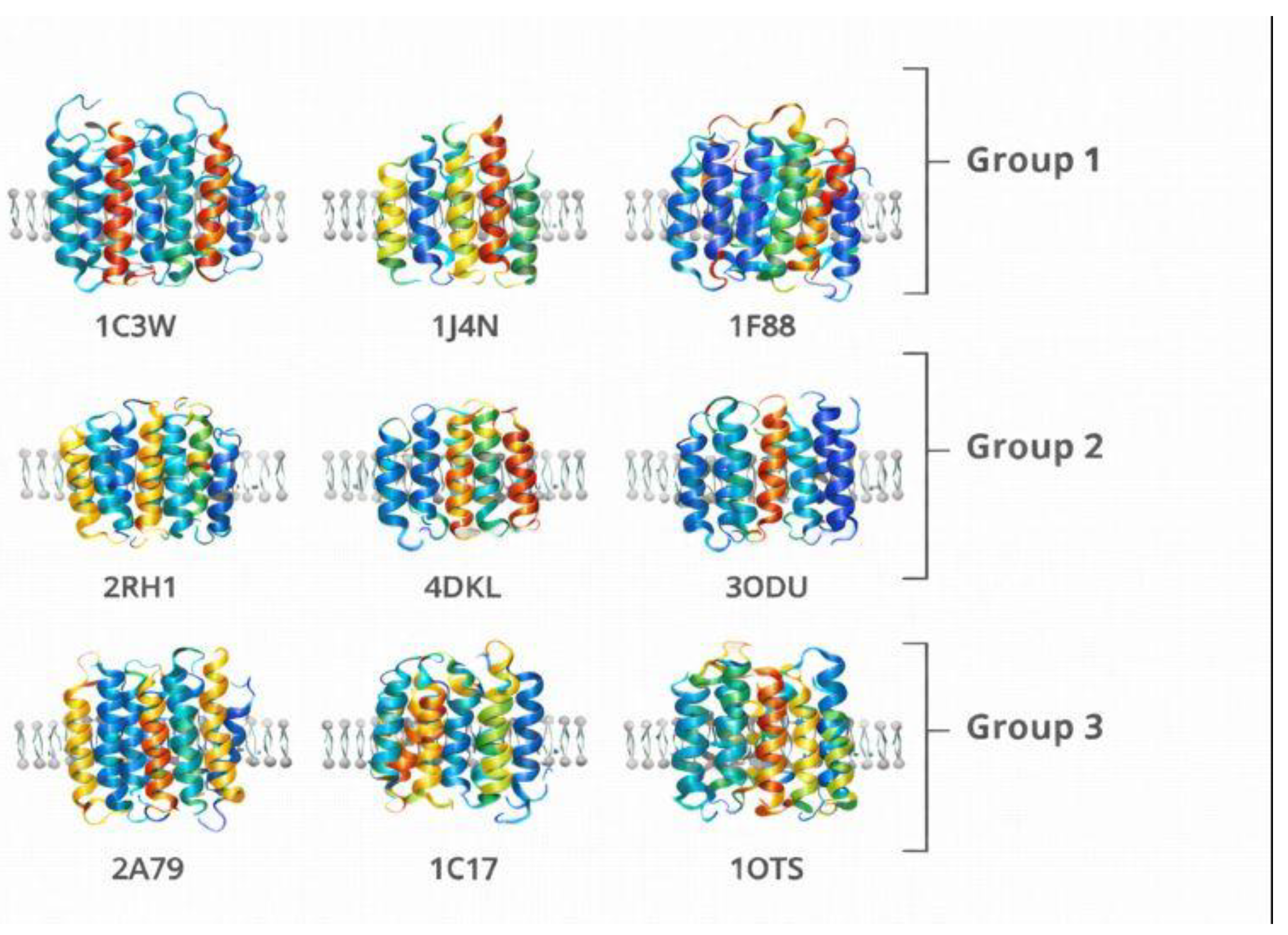
The first group consists of canonical α-helical membrane proteins, including bacteriorhodopsin (PDB: 1C3W) [45], aquaporin-1 (PDB: 1J4N) [46], and rhodopsin (PDB: 1F88) [47]. These proteins are characterized by their predominantly helical and symmetric architectures, making them ideal for benchmarking fundamental descriptors such as Local Tetrahedral Asymmetry (LTA), Helical Path Curvature (HPC), and Orientation Twist Score (OTS). Their regular geometry ensures a controlled environment for isolating chirality features associated with secondary structure coherence and minimal embedding complexity.
The second group targets G protein-coupled receptors (GPCRs) and other asymmetric membrane proteins that display complex folding patterns and pronounced directional embedding. Structures such as the β2-adrenergic receptor (PDB: 2RH1) [48], the μ-opioid receptor (PDB: 4DKL) [49], and the chemokine receptor CXCR4 (PDB: 3ODU) [50] offer a rich testing ground for descriptors sensitive to asymmetric packing and membrane insertion patterns. These proteins are particularly valuable for evaluating the Asymmetric Environment Score (AES), Depth Distribution Profile (DDP), and Leaflet Asymmetry Index (LAI), as they often exhibit distinct biases in their cytoplasmic and extracellular domains, linked to their signaling roles.
The third group comprises structurally irregular or topologically complex membrane proteins that challenge conventional symmetry and packing assumptions. This set includes the voltage-gated potassium channel (PDB: 2A79) [51], the ATP synthase subunit c (PDB: 1C17) [52], and the ClC chloride transporter (PDB: 1OTS) [53]. These proteins feature mixed secondary structures, twisted domains, and unconventional embeddings, serving as robust test cases for stress-testing the generalizability and robustness of the Chirobiophore descriptors under atypical conditions.
Each protein will be analyzed by computing its full Chirobiophore vector, comprising LTA, HPC, AES, DDP, LAI, and OTS, after alignment along a consistent membrane-normal axis (typically Z). The resulting vectors will be projected into lower-dimensional space using techniques such as principal component analysis (PCA) or t-distributed stochastic neighbor embedding (t-SNE) to visualize clustering behavior. This analysis will determine whether proteins with similar chirality profiles cluster by structural class, functional role, or evolutionary lineage (Supplementary Materials S1).
Figure 12.
Representative membrane protein structures analyzed in this study. Ribbon representations of the nine membrane proteins analyzed in this study, grouped into canonical α-helical proteins (Group 1), GPCRs and asymmetric membrane proteins (Group 2), and structurally complex membrane proteins (Group 3). Structures are shown in membrane-aligned orientation to illustrate architectural diversity relevant to the Chirobiophore analysis.
Optionally, selected proteins may also be subjected to molecular dynamics (MD) simulations to evaluate the temporal stability and variability of Chirobiophore vectors over time. This dynamic validation could reveal trajectory patterns, conformational switches, or topological transitions within chirality space, further underscoring the biological relevance of the descriptors.
Through this structured and biologically diverse benchmark, we aim to demonstrate the utility, interpretability, and discriminatory power of the Chirobiophore framework across a range of real-world macromolecular systems.
4.1. Computational Overview
All Chirobiophore descriptors are computed directly from atomic coordinates extracted from Protein Data Bank (PDB) structures using a standardized, coordinate-invariant workflow. Briefly, each structure undergoes (i) preprocessing and alignment relative to a membrane reference frame, (ii) descriptor-specific geometric analysis at local, mesoscopic, and global scales, and (iii) normalization to ensure comparability across structures of different sizes and topologies.
The complete computational pipeline follows the sequence: PDB preprocessing → membrane alignment → descriptor computation → normalization → vector assembly, resulting in a six-dimensional Chirobiophore vector C = [LTA, HPC, AES, DDP, LAI, OTS]
All steps are deterministic and independent of residue labeling, atom naming conventions, or global coordinate orientation.
4.2. Structure Preprocessing and Coordinate Alignment
Prior to descriptor computation, all structures were stripped of solvent molecules and non-protein heteroatoms unless explicitly required for a given descriptor. Atomic coordinates were translated so that the protein center of mass coincided with the origin.
For membrane proteins, a membrane reference frame was defined by aligning the principal axis of transmembrane helices with the global z-axis, corresponding to the membrane normal. When available, experimentally annotated membrane orientations were used; otherwise, the transmembrane axis was inferred using helix principal component analysis.
All subsequent descriptor calculations are invariant under rigid-body rotation and translation.
The following algorithm was used:
| Algorithm 1: Chirobiophore Descriptor Pipeline |
| Input: PDB structure Output: Chirobiophore vector C = [LTA, HPC, AES, DDP, LAI, OTS] Load atomic coordinates from PDB file Remove solvent and optional heteroatoms Align structure to membrane reference frame (z-axis = membrane normal) For each descriptor did_idi: a. Compute raw geometric measure b. Apply descriptor-specific normalization Assemble normalized values into vector CCC (Optional) Standardize CCC for multivariate analysis |
| Algorithm 2: LTA Computation |
| Input: Atomic coordinates Identify valid tetrahedra (central atom + 3 neighbors) Compute signed tetrahedral volumes Average signed volumes over structure Normalize by mean absolute volume |
| Algorithm 3: HPC Computation |
| Input: Cα backbone coordinates Extract contiguous four-residue backbone segments Compute torsion angle for each segment Assign sign based on handedness Average torsion values over all segments |
| Algorithm 4: AES Computation |
| Input: Atomic coordinates Define local neighborhood for each atom (cutoff radius) Construct angular distribution of neighbors Compute Shannon entropy of angular histogram Average entropy values across atoms |
| Algorithm 5: DDP Computation |
| Input: Atomic coordinates aligned to membrane normal Bin atoms along z-axis Compute normalized density profile Calculate skewness of density distribution |
| Algorithm 6: LAI Computation |
| Input: Atomic coordinates, membrane midplane Partition atoms into upper and lower half-spaces Count atoms (or weighted chirality values) per leaflet Compute normalized difference between leaflets |
| Algorithm 7: OTS Computation |
| Input: Transmembrane helix axes Compute helix axis vectors Measure tilt angles relative to membrane normal Assign handedness from backbone torsion Compute signed average tilt |
4.3. Chirobiophore Descriptor Definitions
Each Chirobiophore descriptor captures a distinct geometric manifestation of chirality and is computed using explicitly defined mathematical operations and parameters, as summarized below. Unless otherwise stated, all descriptors are normalized to yield dimensionless quantities suitable for cross-structure comparison.
LTA values were normalized by the mean absolute tetrahedral volume computed across the structure, ensuring scale invariance with respect to protein size and resolution. HPC was computed over contiguous backbone segments using Cα atoms only, with torsion values averaged over all valid four-point paths; the final score represents the signed mean torsional curvature per residue. For AES computation, angular space was discretized into uniform bins (Δθ = 15°), and Shannon entropy was calculated for each atomic neighborhood within a fixed cutoff radius of 6 Å. Density profiles were normalized by total atom count prior to skewness calculation, ensuring comparability between structures of different sizes. When explicit lipid atoms were not present, LAI was computed using protein atom distributions relative to the membrane midplane, with this limitation explicitly acknowledged in the interpretation. OTS was computed as the signed mean tilt angle of transmembrane helices relative to the membrane normal, with handedness determined from backbone torsion sign conventions.
4.4. Chirobiophore Descriptor Definitions
Each Chirobiophore descriptor captures a distinct geometric manifestation of chirality and is computed using explicitly defined mathematical operations and parameters, as summarized below. Unless otherwise stated, all descriptors are normalized to yield dimensionless quantities suitable for cross-structure comparison.
LTA values were normalized by the mean absolute tetrahedral volume computed across the structure, ensuring scale invariance with respect to protein size and resolution. HPC was computed over contiguous backbone segments using Cα atoms only, with torsion values averaged over all valid four-point paths; the final score represents the signed mean torsional curvature per residue. For AES computation, angular space was discretized into uniform bins (Δθ = 15°), and Shannon entropy was calculated for each atomic neighborhood within a fixed cutoff radius of 6 Å. Density profiles were normalized by total atom count prior to skewness calculation, ensuring comparability between structures of different sizes. When explicit lipid atoms were not present, LAI was computed using protein atom distributions relative to the membrane midplane, with this limitation explicitly acknowledged in the interpretation. OTS was computed as the signed mean tilt angle of transmembrane helices relative to the membrane normal, with handedness determined from backbone torsion sign conventions.
To allow direct comparison between structures, all descriptor values were normalized either by intrinsic geometric scales (e.g., mean volume, atom count) or by statistical standardization across the dataset. The resulting dimensionless descriptors were assembled into the final Chirobiophore vector without additional weighting unless explicitly stated.
4.5. Reproducibility and Data Availability
All Chirobiophore descriptors reported in this study are computed using deterministic algorithms applied directly to atomic coordinates obtained from publicly available Protein Data Bank (PDB) structures. To ensure full reproducibility, all scripts used for structure preprocessing, membrane alignment, descriptor computation, normalization, and figure generation will be made publicly available in an open-access repository upon revision.
The repository will include source code, input structure lists (PDB IDs), parameter files, example execution workflows, and reference outputs corresponding to the results reported in this manuscript.
The set of membrane protein structures analyzed in this study was intentionally selected to span multiple architectural and functional classes, including canonical α-helical membrane proteins, G protein–coupled receptors, and topologically complex transporters and channels. This selection was designed to provide structural diversity rather than statistical completeness, allowing us to assess whether the proposed descriptors respond meaningfully to qualitatively different forms of macromolecular chirality.
A primary limitation of the present study is the relatively small number of analyzed structures. As a result, the observed clustering patterns and descriptor distributions should not be interpreted as statistically definitive classifications of membrane protein chirality. Instead, they demonstrate the feasibility and discriminatory potential of the Chirobiophore framework when applied to structurally diverse examples.
Comprehensive validation across larger datasets will be required to establish population-level trends, confidence intervals, and class-specific thresholds for individual descriptors.
The dataset is not intended to exhaustively sample membrane protein space, but rather to serve as a representative proof-of-concept benchmark for evaluating descriptor behavior across distinct structural regimes.
From a computational perspective, the Chirobiophore framework is inherently scalable, as each descriptor is computed independently from atomic coordinates with linear or near-linear complexity in system size. Extension to larger datasets or ensemble-based analyses therefore requires no modification of the underlying methodology.
All computational steps follow a modular workflow in which individual descriptors can be computed independently or jointly assembled into a Chirobiophore vector. This modularity enables straightforward reproduction of individual results and facilitates future extension of the framework to additional descriptors or datasets.
The present study focuses on deterministic descriptor values computed from individual static protein structures and does not yet incorporate ensemble-based variability, experimental uncertainty, or conformational sampling. As such, reported Chirobiophore values should be interpreted as structure-specific descriptors, not as population means or statistically converged estimates.
Descriptor comparisons presented in this section reflect relative differences between proteins within the analyzed dataset and are intended to illustrate trends rather than establish statistically significant separations between protein classes. No assumptions of normality or class-level distributions are made at this stage.
Sensitivity of the Chirobiophore descriptors to coordinate alignment, binning resolution, and neighborhood cutoffs was qualitatively assessed to ensure numerical stability. Descriptor definitions were chosen to minimize dependence on arbitrary parameter choices, and future work will include systematic sensitivity analyses to quantify parameter-induced variance.
Because the present analysis is based on a limited number of static structures, the study does not yet provide confidence intervals, variance estimates, or hypothesis tests for individual descriptors. Consequently, observed clustering patterns and gradients should be interpreted as qualitative indicators of descriptor behavior rather than statistically validated separations. Establishing statistical robustness will require larger datasets and ensemble-based analyses.
Future extensions of the Chirobiophore framework will incorporate statistical characterization of descriptor distributions across protein families, uncertainty estimates derived from conformational ensembles (e.g., molecular dynamics trajectories), and formal hypothesis testing where appropriate. These developments will enable rigorous assessment of descriptor robustness and biological relevance.
4.6. Descriptor Definitions
To capture the distributed and emergent nature of chirality in biological macromolecules, particularly membrane proteins, we introduce a suite of geometric descriptors. These descriptors form the components of the Chirobiophore vector, a multiscale, orientation-invariant representation of structural asymmetry. Each descriptor targets a specific scale or mode of chirality, from local atomic arrangements to global membrane-spanning geometry.
We begin by formally defining three core descriptors: Local Tetrahedral Asymmetry (LTA), Helical Path Curvature (HPC), and the Asymmetric Environment Score (AES). Each provides unique geometric insight into different layers of chiral structure.
Local Tetrahedral Asymmetry (LTA)
Purpose:
LTA quantifies the local handedness of atomic arrangements by evaluating the signed volume of tetrahedra formed by a central atom and three of its bonded neighbors. This descriptor captures chirality at the finest structural scale—atomic geometry.
Mathematical Definition:
Given four atoms with positions r⃗i, r⃗j, r⃗k, r⃗l, the signed volume of the tetrahedron they form is:
The sign of this volume indicates the handedness (left or right) of the local configuration. LTA is then computed as the normalized average of signed volumes across all valid tetrahedra in the system:
where V− is a normalization factor (e.g., mean absolute volume) and N is the total number of tetrahedra considered.
Helical Path Curvature (HPC)
Purpose:
HPC assesses global chirality along polymer backbones, such as protein α-helices, by evaluating the cumulative sign of torsion angles over sequential four-atom paths. This descriptor detects the dominant handedness of chains or folds.
Mathematical Definition:
For a four-atom segment with positions r⃗1, r⃗2, r⃗3, r⃗4 define:
b→1 = r→2− r→1
b→2 = r→3− r→2
b→3 = r→4− r→3
From these, compute two normal vectors:
n→1 = b→1× b→2
n→2 = b→2× b→3
Then, the torsion angle θ is:
θ =
arctan2(∥b→2∥⋅(b→1⋅n→2), n→1⋅n→2)
The sign of θ determines the loca l handedness of that segment. The overall descriptor is computed as:
where
M
M is the number of four-atom paths (typically along backbone or helical axes).
Asymmetric Environment Score (AES)
Purpose:
AES captures the degree of spatial asymmetry in the local environment around each atom. It is beneficial for detecting irregular or functionally diverse regions, such as protein–lipid interfaces or disordered loops. Mathematical Definition: For a given atom i, the AES is derived from the angular distribution of its neighboring atoms. This distribution is converted into a probability histogram over angular bins k, producing normalized values pik:
where Hik is the number of neighbors in bin k, the local entropy is then:
The final AES is the average entropy across all atoms:
Low entropy implies highly symmetric local environments; high entropy reflects asymmetric or heterogeneous packing.
Directional Density Profile (DDP)
Purpose:
DDP characterizes the anisotropic distribution of atomic density along a given axis, typically aligned with the membrane normal. This descriptor is especially suited for membrane proteins, where asymmetry often emerges along the direction perpendicular to the bilayer plane. Mathematical Definition: Let zzz denote the coordinate along the chosen axis (e.g., membrane normal). The spatial domain is partitioned into a set of evenly spaced slabs (or bins) along zzz. For each bin bbb, count the number of atoms nbn_bnb residing within it to generate a density profile ρ(zb)\rho(z_b)ρ(zb). The DDP is then computed as a skewness metric of this distribution:
where:
μis the mean position of the density distribution,
σis the standard deviation,
N is the total number of bins,
Nb is the atom count in bin b,
zb is the central coordinate of bin b.
A nonzero skewness indicates an asymmetric distribution of matter along the axis, consistent with chiral asymmetry.
Lipid Asymmetry Index (LAI)
Purpose: LAI is designed to detect asymmetry in the composition and arrangement of lipids around membrane proteins. Since proteins often interact unevenly with the inner vs. outer leaflets of the membrane, LAI provides a scalar summary of this bias.
In the present study, the Leaflet Asymmetry Index (LAI) was computed without explicit lipid bilayers, as most analyzed Protein Data Bank structures do not contain fully resolved membrane environments. Instead, LAI was derived from the spatial distribution of protein atoms relative to an inferred membrane midplane.
Specifically, following alignment of the protein to a membrane reference frame, the structure was partitioned into two half-spaces along the membrane normal (z = 0). Protein atoms (or residue centroids) located at z > 0 were assigned to the upper leaflet proxy, while those at z < 0 were assigned to the lower leaflet proxy. LAI was then computed as the normalized difference in atom counts between these two regions. While this formulation does not measure lipid compositional asymmetry, it captures protein embedding asymmetry with respect to the membrane plane. As such, LAI should be interpreted as a descriptor of structural leaflet bias of the protein itself, rather than as a direct measure of bilayer lipid asymmetry. Because explicit lipid bilayers were not included, LAI values reported here do not reflect lipid–protein compositional asymmetry or leaflet-specific lipid interactions. Consequently, LAI should be interpreted as a geometric proxy for protein orientation and depth bias within the membrane rather than as a direct measurement of membrane asymmetry. Future implementations of LAI may incorporate explicit lipid coordinates derived from co-crystallized structures, membrane modeling tools, or molecular dynamics simulations, enabling direct quantification of lipid–protein leaflet asymmetry. Such extensions would allow separation of protein-intrinsic embedding bias from bilayer compositional effects.
Mathematical Definition: Consider two regions flanking the membrane midplane—typically corresponding to the cytoplasmic and extracellular (or periplasmic) leaflets. Let Nupper and Nlower represent the number of lipid atoms, headgroups, or residues in the respective regions within a fixed radius of the protein. The LAI is defined as:
Values range from −1 to 1:
LAI = 0 implies perfect symmetry,
LAI > 0 implies more lipids in the upper region,
LAI < 0 implies more in the lower region.
This descriptor can also be generalized to compare specific lipid species, charge distributions, or interaction energies.
Orientation Tensor Skew (OTS)
Purpose: OTS measures the geometric asymmetry of the mass or shape distribution by analyzing the skew of the orientation (or inertia) tensor. It captures the global handedness of a 3D object beyond specific local features.
Mathematical Definition: Construct the orientation tensor T\mathbf{T}T based on all atomic positions r⃗i\vec{r}_iri, typically centered on the center of mass:
where:
α,β ∈ {x,y,z},
wi_ is a weighting factor (e.g., atomic mass or uniform),
rˉα is the center-of-mass coordinate along axis α
Compute the eigenvalues λ1, λ2, λ3 of T, ordered such that λ1 ≤ λ2 ≤ λ3. The skew of this spectrum reflects anisotropic elongation or flattening. Define the skewness as:
A high positive or negative OTS indicates directional shape asymmetry that can arise from twisted or irregular geometries—hallmarks of chiral macromolecular architecture.
Cₒ = [LTA, HPC, AES, DDP, LAI, OTS}
This vector captures a hierarchy of chiral features:
Local (atomic level): LTA, AES
Mesoscale (secondary structure): HPC
Membrane-scale (orientation and embedding): DDP, LAI
Global (shape and symmetry): OTS
By design, the Chirobiophore vector is frame-invariant and scale-aware, allowing for the quantitative comparison of chirality across proteins with diverse sizes, folds, and membrane orientations. It serves as the foundation for downstream tasks such as embedding analysis, classification, and structure-function correlation.
4.7. Membrane Comparison Descriptors
In addition to intrinsic chirality descriptors that apply broadly across biological macromolecules, membrane-associated proteins exhibit distinct geometric and topological asymmetries arising from their spatial embedding within lipid bilayers. Traditional stereochemical measures or secondary-structure-based indices do not fully capture these asymmetries. To address this, we define a suite of membrane comparison descriptors that quantify how chirality is expressed and explicitly modulated in the context of the membrane environment. These descriptors include the Depth Distribution Profile (DDP), the Leaflet Asymmetry Index (LAI), and the Orientation Twist Score (OTS). Each of these components captures different aspects of how structure and chirality are distributed relative to the bilayer’s spatial and functional axes.
4.7.1. Depth Distribution Profile (DDP)
Conceptual Basis: The Depth Distribution Profile (DDP) captures how atoms or residues are distributed along the membrane’s normal vector—usually taken as the Z-axis in membrane-aligned coordinate systems. It quantifies asymmetry in insertion depth, which may reflect polarized function, selective exposure, or directional embedding [54].
Computational Method: Let be the Z-coordinates of all relevant atoms or residue centroids (e.g., Cα atoms). We define a normalized histogram P(z) that represents the density of atoms across the bilayer:
where Nk = number of atoms in bin k
The central tendency and spread of this distribution are characterized by the first three moments:
Mean
μz: The expected value (mean) of the random variable z.
zk: A specific value that the variable z can take.
P(zk): The probability that z takes the value zk
The sum is the overall possible value of zk.
Skewness (asymmetry of distribution):
where:
μz: The mean (expected value) of the random variable z, computed as
σz: The standard deviation of z, computed as
zk: Possible values of the random variable.
P(zk): The probability of value zk.
Kurtosis (peakedness):
where:
zk are discrete depth values,
P(zk) is the probability (or frequency) of zk
μz is the mean (expected depth)
σz is the standard deviation of the depth values.
The DDP score can be taken as a vector or scalar combination of these statistics, providing a compact representation of depth-based asymmetry:
DDP = [μz, Skewness, Kurtosis], This vector captures:
μz: Central tendency (average depth)
Skewness: Asymmetry of depth values
Kurtosis: Peakedness and tail heaviness
To reduce this 3D descriptor to a scalar—useful for ranking, similarity, or thresholding the Euclidean norm of the DDP vector can be computed:
This scalar serves as a compact score reflecting the overall statistical shape of the depth profile.
4.7.2. Leaflet Asymmetry Index (LAI)
Conceptual Basis: Many membrane proteins exhibit leaflet-specific distributions of structural features, such as loops, charged residues, or cofactor sites. This asymmetry aligns with biological polarity (e.g., apical vs. basal surfaces) and underlies phenomena like signal propagation, ion gating, or vesicle fusion. The Leaflet Asymmetry Index (LAI) quantifies the imbalance in chiral center or motif density across the upper and lower leaflets of the membrane [55].
Definition: Partition the protein structure using the membrane midplane (typically z = 0 z = 0 z = 0) into:
Upper leaflet (extracellular): zi > 0 z_i > 0 zi > 0
Lower leaflet (cytoplasmic): zi < 0 z_i < 0 zi < 0
Let NupperN_{\text{upper}}Nupper and NlowerN_{\text{lower}}Nlower be the number of identified chiral centers (or other motifs) in the upper and lower membrane regions, respectively (partitioned by the membrane midplane, typically at z = 0 z = 0 z = 0).
Then the LAI is defined as:
Interpretation:
LAI = 0 → symmetric distribution
LAI > 0 → extracellular bias
LAI < 0 → cytoplasmic bias
Extensions: Weighted versions of LAI can account for chirality magnitude (e.g., LTA or AES values), using:
This is a weighted Leaf Asymmetry Index (LAI_weighted), based on chirality scores at different sites. The formula is:
where:
is the chirality score at site i
“upper” refers to sites where the chirality is considered upper-handed (e.g., right-handed, clockwise, or another designated category)
“lower” refers to sites with lower-handed chirality (e.g., left-handed, counterclockwise, or the opposite category)
Interpretation:
The numerator represents the net chirality bias, or the difference in the total score between the upper and lower groups.
The denominator represents the total chirality signal, which is the sum of both upper and lower scores.
The output will always be between −1 and 1, where:
1 means all signals are upper-handed
−1 means all signals are left-handed
0 means a perfect balance between upper and lower
4.7.3. Orientation Twist Score (OTS)
Conceptual Basis: Transmembrane helices often adopt cumulative torsional orientations, creating large-scale helical bundles or asymmetric packing arrangements. The Orientation Twist Score (OTS) measures the net angular rotation or torsional deformation across the bilayer, revealing membrane-spanning chirality trends. Orientation Twist Score (OTS), which quantifies the average directional tilt of membrane-spanning helices in a protein, weighted by their handedness [56].
Mathematical Definition: Let a unit vector represent each transmembrane helix v⃗i connecting its entry and exit points across the membrane (e.g., from the intracellular to the extracellular leaflet). Let θi be the twist angle of helix i, defined as the angle between the local helix axis and the global membrane normal z computed via:
θi = arccos(v→i⋅z^)
v⃗i: unit vector along the axis of the ith helix
z^: unit vector in the membrane normal direction (usually taken as the z-axis)
So, θi is the angle between the helix and the membrane normal.
si = sign(torsioni)
This indicates whether the helix rotates right-handedly (+1) or left-handedly (−1), based on its torsion (e.g., derived from Cα backbone dihedrals).
Orientation Twist Score (OTS)
n: number of membrane-spanning helices
si⋅θi: combines direction (handedness) and tilt magnitude
So OTS is the signed average tilt: right-handed tilts contribute positively, left-handed tilts negatively.
Furthermore: si = sign(torsioni)
torsioni refers to the backbone torsion of the ith membrane-spanning helix.
This torsion is typically computed from the dihedral angles along the Cα (alpha carbon) trace of the helix.
The sign of the torsion indicates the handedness of the helix:
si = +1: right-handed rotation
si = −1: left-handed rotation
Alternative Vectorial Formulation:
If we define twist vectors ⃗tᵢ in 3D space representing helical direction and rotation, a vectorial OTS can be calculated as:
The magnitude ∥OTS⃗∥ then reflects total twist intensity, while its direction encodes the net handedness axis.
Integration with the Chirobiophore
Together, the DDP, LAI, and OTS form a membrane-specific chirality subspace that complements the atomic- and fold-level descriptors (LTA, HPC, AES). These three descriptors provide essential insight into how chirality manifests across and within the bilayer, enabling a comparison of embedded systems in a biologically meaningful, geometry-aware manner [57].
The full Chirobiophore vector, extended to include these descriptors, is therefore:
C = [LTA, HPC, AES, DDP, LAI, OTS]
This 6-dimensional coordinate situates each membrane protein within a chirality space that captures both internal folding asymmetries and bilayer-related structural features.
The 6-dimensional Chirobiophore space provides a structured, composite framework that captures both molecular-level and membrane-level chirality features of a membrane protein. This space is defined by six key descriptors: LTA (Local Torsion Asymmetry), HPC (Helical Polarity Coherence), AES (Asymmetric Embedding Score), DDP (Directional Density Profile), LAI (Lipid Alignment Index), and OTS (Orientation Twist Score).
At the atomic scale, LTA quantifies asymmetry in local torsional angles across the protein backbone. A higher LTA value indicates more pronounced local geometric asymmetry, reflecting subtle chiral patterns in the fold. HPC operates at the fold level, capturing the alignment and handedness coherence of helical domains. Proteins with high HPC values exhibit consistent chiral architectures, such as uniformly right-handed α-helices. AES bridges the fold and membrane interface, measuring how asymmetrically a protein embeds into the lipid bilayer. High AES values suggest biased insertion or a tilted orientation relative to the membrane normal [58,59,60].
At the membrane level, DDP quantifies the distribution of protein mass along the membrane axis. It highlights structural tilt or density shifts within the bilayer. LAI focuses on the interface between membrane lipids and the protein, capturing the correlation between lipid tail orientation and protein structural features. A high LAI reflects a chiral alignment between lipids and the embedded protein. OTS, or Orientation Twist Score, is a vectorial measure that represents the average direction and intensity of twist across the bilayer. Its magnitude reflects the degree of twist, while its direction encodes the net handedness axis of the system [61].
Each protein can be represented as a unique point in this 6-dimensional space, with its coordinates [LTA, HPC, AES, DDP, LAI, OTS] [LTA, HPC, AES, DDP, LAI, OTS] [LTA, HPC, AES, DDP, LAI, OTS] forming a “chiral fingerprint.” The distance between points in this space reflects the similarity or divergence in chirality between proteins. Notably, the dimensions can be grouped conceptually: LTA, HPC, and AES capture fold-level chirality, while DDP, LAI, and OTS characterize membrane-level chirality. Together, these descriptors provide a comprehensive, geometry-aware representation of protein chirality in biologically relevant contexts [62].
4.8. Implementation
Each descriptor within the Chirobiophore framework is derived directly from the geometric structure of membrane proteins, as represented in their PDB (Protein Data Bank) coordinates. Notably, the calculation of these descriptors is performed independently of atom naming conventions, residue labels, or global coordinate frames. This design ensures that the framework remains robust across diverse protein structures and free from bias introduced by arbitrary orientation or labeling.
The Local Torsion Asymmetry (LTA) is computed using signed scalar triple products applied to backbone segments. This approach captures the handedness of local geometries by evaluating the chirality of atomic triplets, making it sensitive to subtle asymmetries in torsion angles along the protein chain.
For the Helical Polarity Coherence (HPC), the method involves computing the arctangent of vectors formed by normal vectors to planes defined by torsion angles. This descriptor quantifies the degree to which the helices maintain a consistent rotational sense, allowing for the detection of coherent chiral alignment across secondary structural elements.
The Asymmetric Embedding Score (AES) is derived from angular entropy. Specifically, it involves generating 2D or 3D angular histograms of protein atoms projected into bilayer-aligned coordinate systems. The entropy of these histograms then serves as a measure of how symmetrically or asymmetrically the protein is embedded relative to the membrane plane. A high entropy score corresponds to a more asymmetric orientation, revealing structural biases that may reflect functional asymmetry.
Membrane-level descriptors use spatially aware vector-based methods. The Directional Density Profile (DDP) is computed using projections of protein atom densities along the membrane normal, analyzed within sliding spatial windows that follow the bilayer axis. This approach detects longitudinal asymmetries, such as domain tilting or biased mass distributions.
The Lipid Alignment Index (LAI) measures the correlation between vectors representing lipid tail orientations and local protein geometry. By projecting both lipid and protein vectors into a membrane-centered frame, LAI captures how well lipid molecules align with chiral protein features—an indicator of structural compatibility and possible chiral induction at the interface.
Finally, the Orientation Twist Score (OTS) is determined by aggregating local twist vectors (each representing a helical direction and rotation) across the protein’s transmembrane domains. These vectors are averaged to produce a single vectorial quantity, where the magnitude reflects the overall twist intensity and the direction encodes the net handedness axis of the embedded protein.
Together, these computation methods enable automated, geometry-aware chirality analysis of membrane proteins that is scalable, label-agnostic, and sensitive to both local and global asymmetries. The resulting Chirobiophore vectors provide a powerful tool for comparative analysis, classification, and interpretation of membrane protein architecture in biologically meaningful terms [63,64,65,66].
4.9. Chirobiophore Vector
The Chirobiophore vector represents the core output of this framework, encapsulating the multidimensional nature of chirality in membrane proteins in a concise and interpretable format. This six-dimensional vector serves as a geometric and functional fingerprint, allowing for meaningful comparison, classification, and analysis of membrane protein structures based on chirality-specific features.
Formally, the vector is defined as:
C = [LTA, HPC, AES, DDP, LAI, OTS]
Each element of this vector corresponds to one of the six descriptors introduced previously, selected to span both atomic-level and membrane-level structural asymmetries. The components are computed from intrinsic geometry and are independent of atom names, residue labels, or protein orientation, making the vector robust and generalizable across diverse datasets.
4.9.1. Fold-Level Components
Local Torsion Asymmetry (LTA): Quantifies fine-grained chirality at the atomic level by measuring asymmetry in torsion angles along the protein backbone. This is particularly sensitive to local structural irregularities and provides insight into intrinsic folding asymmetries, regardless of the membrane context.
Helical Polarity Coherence (HPC): Measures the consistency and alignment of helical elements with respect to their rotational polarity. A high HPC indicates that the helices share a common handedness and orientation, reflecting global fold regularity and potential functional coherence.
Asymmetric Embedding Score (AES): Captures the orientation and placement of the protein within the lipid bilayer by measuring entropy from angular histograms in membrane-aligned coordinates. A higher AES signifies a greater deviation from symmetric embedding, which can reflect biological phenomena such as unidirectional signaling or asymmetric domain exposure [58].
4.9.2. Membrane-Level Components
Directional Density Profile (DDP): Reflects how protein mass is distributed along the membrane normal. By computing localized density projections, DDP identifies biases such as structural tilt, lopsided transmembrane domain arrangement, or mass asymmetry between extracellular and cytoplasmic regions.
Lipid Alignment Index (LAI): Evaluates how well the protein’s geometry aligns with the orientation of surrounding lipid tails. This captures protein-lipid interface chirality and may highlight structural adaptations for lipid recognition, stabilization, or modulation.
Orientation Twist Score (OTS): Provides a global measure of twist across the bilayer. It is computed as the vector average of local helical twist directions. The magnitude of OTS reflects the degree of net helical deformation, while its direction encodes the axis of net handedness, offering a holistic view of membrane-twist architecture.
By placing a membrane protein in this six-dimensional space, the Chirobiophore vector characterizes its complete chirality profile, bridging molecular folding properties and membrane interactions. The vector can be used as a coordinate system for comparing proteins: structural similarity in chirality corresponds to proximity in this space. Furthermore, because the Chirobiophore vector supports metric operations, standard techniques such as clustering, principal component analysis, and similarity scoring can be applied.
This enables not just pairwise comparison, but also systematic analysis across protein families, functional groups, or evolutionary lineages, with chirality treated as a first-class structural descriptor. The Chirobiophore space can also be integrated into machine learning workflows, facilitating classification tasks, anomaly detection, and interpretability in structural prediction pipelines.
Notably, the inclusion of both fold-level and membrane-level descriptors ensures that the vector captures the multiscale nature of chirality in membrane proteins—something traditional shape-based or sequence-based methods often overlook. Thus, the Chirobiophore vector stands as a biologically informed, geometrically rigorous tool for advancing our understanding of protein structure, function, and interactions in membrane environments [67,68,69].
4.10. Chirobiophore as a Point in Chirality Space
C = [LTA, HPC, AES, DDP, LAI, OTS] ∈ ℝ6
This forms a 6D coordinate, where each dimension represents a distinct type of chirality or asymmetry. Every structure (protein, membrane, model) is a point in this chirality space.
Each Chirobiophore vector defines a position in a six-dimensional real-valued vector space:
C = [LTA, HPC, AES, DDP, LAI, OTS] ∈ R6
This mathematical formulation situates every protein, membrane-embedded system, or computational model as a single point in a continuous chirality space, where each axis reflects a distinct and biologically interpretable form of asymmetry. In essence, the Chirobiophore vector acts as a coordinate system for quantifying and comparing structural chirality at multiple spatial scales.
Each of the six dimensions—LTA, HPC, AES, DDP, LAI, and OTS—serves as an orthogonal descriptor, contributing independent information about the structure’s handedness. The first three dimensions (LTA, HPC, AES) capture intrinsic asymmetries of the protein’s fold and secondary structure, while the latter three (DDP, LAI, OTS) encode how the protein interacts with and is organized within the lipid bilayer. This split ensures that the space reflects both internal chiral architecture and extrinsic membrane-contextual asymmetry [70,71].
By embedding a protein in this chirality space, its position vector becomes a comprehensive structural signature. Proteins with similar chiral properties will cluster nearby in this space, whereas those with distinct folding or embedding asymmetries will occupy more distant locations. This geometric representation supports both qualitative reasoning (e.g., visualizing chirality shifts) and quantitative analysis (e.g., computing Euclidean or cosine distances between vectors).
Importantly, this abstraction enables a wide range of computational applications:
Clustering and classification: Proteins can be grouped based on proximity in chirality space, facilitating the discovery of structural or functional families that share chiral motifs.
Outlier detection: Unusual structures—such as those resulting from mutations, design errors, or alternate topologies—may occupy sparsely populated or extreme regions of the space.
Time-dependent studies: In simulations, the evolution of a protein’s Chirobiophore vector over time can reveal conformational drift, folding pathways, or membrane reorganization.
Comparative modeling: The Chirobiophore space provides an objective basis for comparing experimental structures to computational models or predictions, offering chirality-based validation metrics [72,73].
Moreover, because each axis of the space is derived from raw geometry, independent of labeling, sequence, or alignment, the representation is broadly applicable across organisms, resolutions, and modeling methods. The vectorization process is also invertible in the sense that a location in chirality space can be mapped back to interpretable physical features (e.g., “this protein has high twist but low polarity coherence”).
In this way, the Chirobiophore space serves not merely as a descriptive tool but as a conceptual framework for exploring the geometry of membrane protein chirality. It bridges the gap between molecular structure and higher-level organization, allowing chirality to be treated as a first-class structural property—measurable, comparable, and computationally actionable.
In addition to its metric and geometric properties, the Chirobiophore space can be understood from a topological perspective, offering a more abstract but powerful layer of interpretation. By treating chirality as a property that is invariant under continuous deformation, topology enables us to reason about structural class, global orientation, and symmetry breaking in ways that transcend local atomic fluctuations or alignment conventions [74].
At its core, the Chirobiophore vector defines a coordinate embedding of protein structures into a real-valued topological vector space, where open sets correspond to regions of similar chirality, and neighborhood structure reflects the continuity of geometric transformation. That is, small perturbations in fold or membrane placement result in continuous changes in the Chirobiophore vector. This continuity ensures the stability of the representation under biologically plausible structural variations—such as domain flexing, side-chain dynamics, or lipid bilayer deformation—preserving topological class membership even when exact geometry changes.
From a topological classification standpoint, proteins that occupy the same connected region (or component) of Chirobiophore space can be interpreted as chirality-homologous—that is, they belong to the same structural chirality class, even if their atomic details differ. This is particularly useful for understanding evolutionary variation, conformational ensembles, or functional switching (e.g., gating in ion channels), where chirality might shift locally but the topological identity remains intact [75].
Moreover, several Chirobiophore components themselves are inherently topological in nature:
HPC reflects winding number consistency, a concept that parallels topological invariants like twist or linking number in knot theory.
OTS encodes net helical handedness direction, acting similarly to an orientation vector in a fiber bundle or a mapping degree in topology.
AES and DDP, though computed geometrically, are sensitive to global asymmetry and can identify transitions across topological barriers—such as inversion or domain flipping—within the bilayer.
These properties make Chirobiophore space especially suited for capturing topological transitions, such as symmetry-breaking events, pseudo-mirror states, or chiral inversion. For example, if a protein undergoes a change in embedding that mirrors its transmembrane domains (as might occur during dimerization or misfolding), this would correspond to movement across a chirality-inverting manifold in the space—a topologically significant shift, even if the total structure remains energetically favorable.
Importantly, because the Chirobiophore space is homeomorphic to R6, it admits continuous mappings, embeddings, and vector field definitions, allowing techniques from topology and differential geometry to be applied. For instance, chirality gradients (i.e., derivatives of Chirobiophore values across spatial or temporal dimensions) can define vector flows or morphogen-like landscapes for structural organization [76,77].
Implications
Understanding the Chirobiophore vector as a topological embedding reinforces its role not just as a structural descriptor but as a model of continuity, class identity, and deformation resilience in membrane protein structure. It allows one to move beyond static comparison toward a dynamical, deformation-aware view of chirality—ideal for modeling folding pathways, membrane transitions, or evolutionary divergence.
This perspective also opens the door to topology-based learning and analysis techniques, such as persistent homology, topological clustering, and manifold learning, which can reveal higher-order structure in the distribution of proteins across Chirobiophore space—discovering not just groups, but also shape in the chirality space itself [78].
4.11. Chirality Manifold: A Curved Shape Space
Imagine all physically possible structures as forming a curved, nonlinear manifold inside ℝ6:
C1 C3
●-----●
/ \
● ●
C2 C4
C1 → C2 → C3 → C4 could represent a developmental transition (e.g., from primitive to specialized endothelial cells).
The curvature shows that not all chirality states are equally likely or accessible.
Although the Chirobiophore vector maps each membrane protein to a point in a six-dimensional Euclidean space (R6\mathbb{R}^6R6), the set of physically realizable protein structures does not fill this space uniformly. Instead, these biologically plausible configurations occupy a curved, lower-dimensional manifold embedded within the larger coordinate space. This conceptual space, referred to as the chirality manifold, represents a continuous, non-linear surface through which proteins can transition via structural deformation, functional adaptation, or evolutionary change.
The chirality manifold reflects the constraints imposed by the biophysics of protein folding, membrane embedding, and functional specialization. Because protein structures are governed by steric limits, thermodynamic feasibility, and membrane interactions, only a subset of all mathematically possible Chirobiophore vectors corresponds to viable molecular configurations. In this view, each protein exists not as an isolated point in R6, but as a location on a smooth, possibly curved hypersurface that defines the space of allowable chiral structures [79,80].
This manifold offers a robust conceptual framework for understanding how chirality evolves and is regulated across various structural, developmental, and evolutionary trajectories. For example, a sequence of states represented by vectors C1 → C2 → C3 → C4 might correspond to a biological transformation, such as the differentiation of membrane-bound receptors in primitive cells into highly specialized forms in vascular endothelium. The pathway across the manifold captures not just discrete chirality values but also their smooth transitions, revealing which structural changes are energetically or evolutionarily accessible.
Importantly, the curvature of the manifold is biologically informative. In regions of low curvature—where the surface is relatively flat—small changes in protein structure lead to proportionally small changes in chirality. These areas represent standard, stable, or low-energy configurations that many proteins may share. In contrast, regions of high curvature indicate rare, transitional, or energetically unfavorable states, where minor geometric perturbations produce significant shifts in chirality. Such regions may correspond to intermediate states during folding, moments of functional switching, or structures prone to instability or misfolding [81].
This topological view also explains why specific chirality profiles are more prevalent or evolutionarily favored than others: proteins tend to occupy broad, accessible regions of the manifold, while highly twisted, asymmetrically embedded, or otherwise extreme configurations are rare and often short-lived. Thus, chirality becomes not just a descriptor, but a constrained evolutionary variable with its own geometric logic.
In parallel to the continuous manifold, a graph-theoretical representation of chirality can be used to capture local structure and connectivity. In this representation, each protein is modeled as a graph, where nodes represent residues or atoms, and edges denote covalent bonds or spatial proximity within a defined cutoff. These edges can be weighted using chirality-relevant metrics—such as Local Torsion Asymmetry (LTA), Asymmetric Embedding Score (AES), or a Side-chain Orientation Coherence (SOC) metric—thus allowing chirality to be encoded into the topology of the graph itself [82].
Analyzing such graphs enables the application of powerful topological data analysis methods. Clustering algorithms can identify recurring chiral motifs, such as twisted β-sheets or helical bundles with consistent handedness. Betti numbers, a concept from algebraic topology, can be computed to count the number of loop-like structures or cavities in the graph, which correspond to structural patterns such as twists, folds, and tunnels. Additionally, persistent homology—a method that tracks how topological features persist across multiple spatial or energetic scales—can reveal stable chiral cores in the protein, distinguishing them from transient or noise-prone conformations.
When combined, the chirality manifold and the graph representation offer a multiscale, dual-view framework for understanding membrane protein chirality. The manifold captures the global, continuous variation of chirality across the protein space, enabling comparative analysis and trajectory modeling. The graph captures local, discrete structure, suitable for motif detection, topological invariants, and structural classification.
Together, these views provide a rich geometric and topological foundation for investigating the role of chirality in protein function, stability, and evolution. They open new avenues for structural prediction, synthetic design, and classification based not only on shape or sequence, but on the profound structural asymmetries that govern how proteins fold, embed, and operate in the membrane environment [83,84,85].
4.12. Chirality Fiber Bundle (Field over Structure)
To move beyond a global, vector-based representation of chirality, we can introduce a fiber bundle model, which conceptualizes chirality not as a single value for an entire protein, but as a distributed field mapped across its structure. In this view, the protein is treated as a base space—a continuous curve or surface defined by its atomic or residue-level geometry—and each point along this base is associated with a local chirality vector, forming a fiber attached to that point.
For example, consider a membrane protein backbone. At each residue iii, one can compute a local chirality descriptor, such as:
Residue i → [LTAi, AESi]
Here, Local Torsion Asymmetry (LTA) and Asymmetric Embedding Score (AES) provide local measures of handedness and membrane asymmetry, respectively. These per-residue vectors form a field of chirality descriptors aligned along the backbone. Visually, this can be imagined as a series of small arrows (vectors) “attached” to each point of the structure, pointing in the direction and magnitude of local chirality:
This construction defines a chirality fiber bundle, in which each “fiber” (the local vector) varies smoothly or discontinuously along the base structure (the protein). The resulting field can be analyzed similarly to a topographic map, revealing patterns of chiral intensity, inversion, or coherence along the structure.
This localized view is handy for studying heterogeneous chirality within proteins—cases where some regions exhibit strong chirality and others are nearly symmetric. It also enables gradient-based analysis, where abrupt changes in vector orientation may signal structural boundaries, hinge points, or transitions between functional domains [86,87].
Protein backbone: ———————>
↖
Local chirality vector
Loops and Bifurcations in Chirobiophore Trajectories
When the Chirobiophore vector is tracked over time, along a conformational pathway, or across evolutionary states, it traces a trajectory through chirality space. These trajectories can exhibit rich geometric and topological structure, including loops, branches, and bifurcations.
A loop in Chirobiophore space occurs when a protein returns to a previous chirality state after undergoing a structural change. This might correspond to reversible transitions, such as those seen in allosteric regulation, conformational switching (e.g., active vs. inactive states of a channel), or cyclical tissue processes like inflammation, repair, and homeostasis. The loop structure in chirality space reflects periodicity or recurrence in the underlying physical system:
●
/ \
●● ●● ← Converging or diverging chirality states
/ \
●● ●● ← Closed loop = reversible or periodic behavior
A bifurcation represents a point at which a single trajectory splits into two or more paths, reflecting a decision point in chirality. This can arise in evolutionary divergence, structural polymorphism, or during protein folding when intermediate states may resolve into distinct final forms. Conversely, convergence occurs when multiple distinct structures evolve toward a common chirality state—perhaps due to functional constraints or shared membrane embedding conditions.
These loop and branching behaviors are not merely mathematical curiosities—they capture biologically meaningful dynamics. For instance, A loop may encode the reversible morphodynamics of a signaling protein toggling between resting and active states. A bifurcation might model tissue-specific adaptation, where the same protein adopts different chiral conformations in different cellular environments. Converging branches could reflect structural convergence, where unrelated proteins adopt similar chiral profiles to interface with a common membrane lipid domain. By analyzing these trajectories within Chirobiophore space, researchers can uncover hidden structure-function relationships, identify points of structural flexibility or constraint, and map out dynamic chirality landscapes that are informative for both biology and design (Table 16). The scripts used to compute and demonstrate the Chirobiophore are attached to Supplementary Materials S1 [88,89,90,91].
Future validation efforts will focus on applying the Chirobiophore framework to expanded membrane protein datasets, including homologous families, conformational ensembles derived from molecular dynamics simulations, and experimentally annotated membrane orientation databases. Such studies will enable statistical characterization of descriptor distributions and more rigorous assessment of robustness and generality.
5. Conclusions
Within this work, we introduced the Chirobiophore framework—a comprehensive, multiscale model for quantifying, analyzing, and interpreting chirality in membrane protein structures. By unifying atomic-level descriptors with membrane-contextual metrics, the Chirobiophore vector enables each protein to be embedded within a six-dimensional space of chirality that is both geometrically precise and biologically meaningful.
The framework captures fold-level asymmetries by constructing descriptors such as Local Torsion Asymmetry (LTA), Helical Polarity Coherence (HPC), and Asymmetric Embedding Score (AES). These are complemented by Directional Density Profile (DDP), Lipid Alignment Index (LAI), and Orientation Twist Score (OTS), which model the protein’s integration into and interaction with the lipid bilayer. Together, these descriptors represent a geometry-aware fingerprint of structural handedness that is robust, continuous, and orientation-independent.
By conceptualizing this chirality space as a nonlinear manifold embedded within R6, we frame structural transitions, evolutionary trajectories, and folding pathways as paths on a curved surface. This topological interpretation reveals the geometric constraints that govern chirality and explains why certain structural states are more probable or stable than others.
We further extended the model by representing proteins as graph structures, in which chirality is distributed across local nodes (residues) and edges (bonds or proximity). This graph-based approach enables the application of topological data analysis, such as clustering, loop detection via Betti numbers, and persistent homology, to uncover recurrent chiral motifs and robust structural patterns.
The concept of a chirality fiber bundle, where local vectors are attached to every point along the protein backbone, enriches this framework by enabling spatially resolved analysis of chirality. Such vector fields can be interpreted as chirality landscapes, analogous to topographic maps, revealing regions of stability, transition, and inversion.
Finally, we demonstrated how Chirobiophore trajectories—paths traced in chirality space over time or across structural ensembles—can reveal loops, bifurcations, and convergence zones, each of which corresponds to meaningful biological phenomena such as reversible conformational switching, folding bifurcations, or functional convergence.
In summary, the Chirobiophore framework not only quantifies chirality across multiple structural levels but also offers a conceptual, mathematical, and computational toolkit for exploring its dynamics and implications. It bridges structural biology with topology, geometry, and machine-readable vectorization, opening new directions for the classification, simulation, and design of membrane proteins based on chirality. This framework may also serve as a foundation for future efforts in structure-based function prediction, protein engineering, and evolutionary modeling, where chirality plays a critical yet often overlooked role.
Supplementary Materials
The following supporting information can be downloaded at: https://www.mdpi.com/article/doi/s1. S1 provides all data and documentation required to reproduce the analyses presented in this manuscript. Specifically, S1 includes: (i) a complete list of all analyzed Protein Data Bank (PDB) structures; (ii) full numeric Chirobiophore descriptor tables (LTA, HPC, AES, DDP, LAI, OTS) for each protein; (iii) preprocessing parameters and normalization schemes used for descriptor computation; (iv) example scripts and pseudo-code illustrating the computational workflow; and (v) additional supporting figures and tables related to descriptor robustness and visualization.
Author Contributions
C.N.L. and S.C.B.; originate the idea of chirobiophore and coin the term, C.N.L. and S.C.B.; software, C.N.L. and S.C.B.; validation, C.N.L. and S.C.B.; formal analysis, C.N.L. and S.C.B.; investigation, C.N.L. and S.C.B.; resources, C.N.L. and S.C.B.; data curation, C.N.L. and S.C.B.; writing—original draft preparation, C.N.L. and S.C.B.; writing—review and editing, C.N.L. and S.C.B.; visualization, C.N.L. and S.C.B.; supervision, C.N.L. and S.C.B.; project administration, C.N.L. and S.C.B. funding acquisition. All authors have read and agreed to the published version of the manuscript.
Funding
Please This research received no external funding.
Institutional Review Board Statement
Not applicable.
Informed Consent Statement
Not applicable.
Data Availability Statement
On reasonable demand.
Acknowledgments
One of the authors (SCB) is highly grateful to Lemont B Kier for his numerous illuminating discussions regarding the process by which he (LBK) originated the idea of pharmacophore.
Conflicts of Interest
The authors declare no conflicts of interest.
Abbreviations
The following abbreviations are used in this manuscript:
| AES | Asymmetric Environment Score |
| API | Anisotropy-Packing Index |
| ABAI | Apicobasal Asymmetry Index |
| CPS | Chirality Persistence Score |
| CGI | Chirality Genus Index |
| CVF | Chirality Vector Field Curl |
| CEI | Chirality Entanglement Index |
| TCC | Topological Chirality Complexity |
| DDP | Directional Density Profile |
| LTA | Local Tetrahedral Asymmetry |
| HPC | Helical Path Curvature |
| LAI | Leaflet Asymmetry Index |
| OTS | Orientation Twist Score |
| MECI | Membrane Embedding Contrast Index |
| TMOI | Transmembrane Orientation Index |
| PSI | Polarity Skew Index |
| RBI | Rotational Bias Index |
| PDI | Packing Disparity Index |
| HRS | Helical Regularity Score |
| TPI | Tissue Polarity Index |
| MCI | Morphogenetic Complexity Index |
| FCI | Functional Chirality Index |
Appendix A
This is a well-structured mathematical description of how morphogenetic indices (like PSI) are computed as linear projections of standardized Chirobiophore descriptors.
Tissular/Cellular Index Computation from Chirobiophore Descriptors
Let the vector of standardized Chirobiophore descriptors be:
Each tissular or cellular index Tk ∈ R is computed as a linear combination of the six standardized descriptors:
where:
wk = [wk,1, wk,2, …, wk,6] ∈ R6 is the weight vector associated with the kth index.
denotes the z-score normalized value of the ith Chirobiophore descriptor.
Example: Polarity Skew Index (PSI)
Given:
wPSI = [0, 0, 0, 0.6, 0.4, 0]
Then:
PSI = 0.6⋅DDP~ + 0.4⋅LAI
General Matrix Form (for Multiple Indices)
For nnn such indices (e.g., PSI, ASI, CSI, etc.), define a projection matrix:
Then the vector of all indices is computed as:
This matrix formulation enables straightforward integration into analytical models, machine learning systems, or mechanistic simulations, allowing protein-level chirality descriptors to be quantitatively linked to tissular or cellular morphogenetic behavior.
References
- Park, Kyung Sun; Xue, Zhengyuan; Patel, Bijal B.; An, Hyosung; Kwok, Justin J.; Kafle, Prapti; Chen, Qian; Shukla, Diwakar; Diao, Ying. Chiral emergence in multistep hierarchical assembly of achiral conjugated polymers . Nature Communications 2022, 13, Article 2738. [Google Scholar] [CrossRef]
- Sallembien, Q.; Plasson, R.; Bersini, H. Possible chemical and physical scenarios towards biological homochirality. Chemical Society Reviews 2022, 51, 803–818. [Google Scholar] [CrossRef]
- Pabst, Georg; Keller, Sandro. Exploring membrane asymmetry and its effects on membrane proteins. Trends Biochem Sci. 2024, 49(4), 333–345. [Google Scholar] [CrossRef]
- Oyewande, O. E.; Neal, M. P.; Low, R. The Hausdorff chirality measure and a proposed Hausdorff structure measure . Molecular Physics 2009, 107(3), 281–291. [Google Scholar] [CrossRef]
- Gómez-Ortiz, F.; Fava, M.; McCabe, E. E.; Romero, A. H.; Bousquet, E. Structural chirality measurements and computation of handedness in periodic solids . Physical Review B 2024, 110, 174112. [Google Scholar] [CrossRef]
- Güner, O. F.; Bowen, J. P. Setting the record straight: the origin of the pharmacophore concept. Journal of Chemical Information and Modeling 2014, 54(5), 1269–1283. [Google Scholar] [CrossRef] [PubMed]
- Schaller, D. Next generation 3D pharmacophore modeling. In WIREs Computational Molecular Science; 2020. [Google Scholar]
- Maeda, I. Scaffold-hopped compound identification by ligand-based methods. Journal of Chemical Information and Modeling, ACS 2024. [Google Scholar] [CrossRef]
- Xia, Kelin; Wei, Guo-Wei. Persistent homology analysis of protein structure, flexibility and folding . PMC. Journal of Computational Chemistry Published via. 2014. [Google Scholar] [CrossRef] [PubMed]
- Schaller, D. Next generation 3D pharmacophore modeling . In WIREs Computational Molecular Science; 2020. [Google Scholar]
- Morehead, A.; Kalia, S.; Ng, J.; Cbib, E.; Singh, S. Geometry-complete perceptron networks for 3D molecular representation learning . Bioinformatics 2024, btae087. [Google Scholar] [CrossRef]
- Xia, C.; Wang, Z.; Liu, Y. Fast protein structure comparison through effective graph-based protein structure representation learning. PLOS Computational Biology 2022, e1009623. [Google Scholar] [CrossRef]
- Salamończyk, M.; Gorecka, E.; Wang, J.; De la Fuente, J. R.; Nakata, M.; Dadj, J.; Geng, X.; Lagerwall, J. P. F. Multi-level chirality in liquid crystals formed by achiral molecules . Scientific Reports 2019, 9, 4375. [Google Scholar] [CrossRef] [PubMed]
- Zhang, D. Y.; et al. Highly Conductive Topologically Chiral Molecular Knots as Efficient Spintronic Chiral Materials. Journal of the American Chemical Society 2023, 145(24), 13472–13481. [Google Scholar] [CrossRef]
- Jamieson, E. M. G.; Modicom, F.; Goldup, S. M. Chirality in rotaxanes and catenanes . Chemical Society Reviews 2018, 47, 5266–5311. [Google Scholar] [CrossRef]
- Pandey, S.; Bera, S.; Gayen, S. Chirality transmission in macromolecular domains . Nature Communications 2022, 13, 4375. [Google Scholar] [CrossRef]
- Wan, L. Q.; Chin, A. S.; Worley, K. E.; Ray, P. Cell chirality: Emergence of asymmetry from cell culture. Philosophical Transactions of the Royal Society B: Biological Sciences 2016, 371(1710), 20150413. [Google Scholar] [CrossRef]
- Alon, Gil; Ben-Haim, Yuval; Tuvi-Arad, Inbal. Continuous Symmetry and Chirality Measures: Approximate Algorithms for Large Molecular Structures. Journal of Cheminformatics 2023, 15, 106. [Google Scholar] [CrossRef]
- Xia, K.; Wei, G.-W. Persistent homology analysis of protein structure, flexibility and folding . International Journal for Numerical Methods in Biomedical Engineering 2014, 30(8), 814–844. [Google Scholar] [CrossRef]
- Shires, Benjamin W.B.; Pickard, Chris J. Visualizing Energy Landscapes through Manifold Learning. Phys. Rev. X 2021, 11, 041026, 5. [Google Scholar] [CrossRef]
- Grason, G. M.; Bruinsma, R. F. Chirality and Equilibrium Biopolymer Bundles . Physical Review Letters 2007, 99(9), 098101. [Google Scholar] [CrossRef]
- Xia, Chen; Wang, Zhenyu; Liu, Yang. Fast protein structure comparison through effective graph-based protein structure representation learning. PLOS Computational Biology 2022, 18(3), e1009623. [Google Scholar] [CrossRef] [PubMed]
- Xia, Kelin; Wei, Guo-Wei. Persistent homology analysis of protein structure, flexibility and folding . International Journal for Numerical Methods in Biomedical Engineering 2014, 30(8), 814–844. [Google Scholar] [CrossRef] [PubMed]
- Edelsbrunner, Herbert; Harer, John. Computational Topology: An Introduction; American Mathematical Society: Providence, RI; ISBN 9780821849255; Betti numbers and Euler characteristic, 2010; p. pp. 55–65 pp. 93–97. [Google Scholar]
- Wietecha, M. S.; Cerny, W. L.; DiPietro, L. A. Mechanisms of vessel regression: toward an understanding of the resolution of angiogenesis . Curr. Top. Microbiol. Immunol. 2013, 367, 3–32. [Google Scholar] [PubMed]
- Cang, Zixuan; Wei, Guo-Wei. Integration of element specific persistent homology and machine learning for protein–ligand binding affinity prediction. International Journal for Numerical Methods in Biomedical Engineering 2017, 33(12), e2914. [Google Scholar] [CrossRef]
- Zając, Sebastian; Geary, Cody; Andersen, Ebbe Sloth; Dabrowski-Tumański, Paweł; Sułkowska, Joanna I.; Sułkowski, Piotr. Genus trace reveals the topological complexity and domain structure of biomolecules. Scientific Reports 2018, 8, 17537. [Google Scholar] [CrossRef]
- Grason, Gregory M. Perspective: Geometry and optimal packing of twisted filaments and fibers. Journal of Chemical Physics 2015, 145(11), 110901. [Google Scholar] [CrossRef]
- Baiesi, M.; Orlandini, E.; Stella, A. Topological and geometrical entanglement in a model of circular DNA undergoing denaturation. European Physical Journal B 2002, 28, 467–473. [Google Scholar] [CrossRef]
- Bernido, C. C.; Carpio-Bernido, M. V.; Aringa, H. P. Topology-dependent entropic differences for chiral polypeptides in solvents. Physics Letters A 2011, 375(9), 1225–1228. [Google Scholar] [CrossRef]
- Kier, L. B. Molecular orbital calculation of preferred conformations of acetylcholine, muscarine, and muscarone. Molecular Pharmacology 1967, 3(5), 487–494. [Google Scholar] [CrossRef] [PubMed]
- Kier, L. B. Molecular Orbital Theory in Drug Research; Academic Press: New York, 1971. [Google Scholar]
- Basak, S. C. The role of mathematical chemodescriptors and proteomics-based biodescriptors in drug discovery. Drug Development Research 72 2010, 1–9. [Google Scholar] [CrossRef]
- Nandy, A.; Harle, M.; Basak, S. C. Mathematical descriptors of DNA sequences: Development and application. ARKIVOC 9 2006, 211–238. [Google Scholar] [CrossRef]
- Guo, X.; Randic, M.; Basak, S. C. A novel 2-D graphical representation of DNA sequences of low degeneracy. Chem. Phys. Lett. 350 2001, 106–112. [Google Scholar] [CrossRef]
- Vracko, M.; Basak, S. C. Similarity study of proteomic maps. Chemometr. Intell. Lab. Syst. 70 2004, 33–38. [Google Scholar] [CrossRef]
- Randic, M.; Witzmann, F.; Vracko, M.; Basak, S. C. On characterization of proteomics maps and chemically induced changes in proteomes using matrix invariants: Application to peroxisome proliferators. Med. Chem. Res. 10 2001, 456–479. [Google Scholar]
- Natarajan, R.; Basak, S. C.; Neumann, T. Multidimensional spaces of numerical chirality descriptors. J. Chem. Inf. Model. 47 2007, 771–775. [Google Scholar] [CrossRef] [PubMed]
- Natarajan, R.; Lungu, C. N.; Basak, S. C. Chirality descriptors for structure–activity relationship modeling of bioactive molecules. J. Math. Chem. 62 2024, 2388–2406. [Google Scholar] [CrossRef]
- Kuhn, T. S. The structure of scientific revolutions; University of Chicago Press, 1962. [Google Scholar]
- Novotni, M.; Klein, R. 3D Zernike descriptors for content based shape retrieval. In Proceedings of the 8th ACM Symposium on Solid Modeling and Applications, 2003; pp. 216–225. [Google Scholar]
- Ramachandran, S.; Kota, P.; Ding, F.; Dokholyan, N. V. Automated minimization of steric clashes in protein structures. Proteins: Structure, Function, and Bioinformatics 2011, 79(1), 261–270. [Google Scholar] [CrossRef]
- Cazals, F.; Dreyfus, T. Beyond pairwise shape comparison: A family of shape metrics from the global point signature. Journal of Computational Chemistry 2017, 38(27), 2040–2050. [Google Scholar]
- White, S. H.; Wimley, W. C. Membrane protein folding and stability: Physical principles. Annual Review of Biophysics and Biomolecular Structure 28 1999, 319–365. [Google Scholar] [CrossRef]
- Luecke, H.; Schobert, B.; Richter, H. T.; Cartailler, J.-P.; Lanyi, J. K. Crystal structure of bacteriorhodopsin mutant D96N in the M intermediate state. Journal of Molecular Biology 1999, 291(4), 899–911. [Google Scholar] [CrossRef]
- Sui, H.; Han, B.-G.; Lee, J. K.; Walian, P.; Jap, B. K. Structural basis of water-specific transport through the AQP1 water channel. Nature 414 2001, 872–878. [Google Scholar] [CrossRef]
- Palczewski, Krzysztof; Kumasaka, Tomomi; Hori, Takashi; Behnke, C. A.; Motoshima, H.; Fox, B. A.; Le Trong, I.; Teller, D. C.; Okada, T.; Stenkamp, R. E.; Yamamoto, M.; Miyano, M. Crystal Structure of Rhodopsin: A G Protein-Coupled Receptor. Science 2000, 289, 739–745. [Google Scholar] [CrossRef]
- Cherezov, V.; Rosenbaum, D. M.; Hanson, M. A.; Rasmussen, S. G.; Thian, F. S.; Kobilka, T. S.; Choi, H. J.; Kuhn, P.; Weis, W. I.; Kobilka, B. K.; Stevens, R. C. High-resolution crystal structure of an engineered human β2-adrenergic G protein-coupled receptor. Science 318 2007, 1258–1265. [Google Scholar] [CrossRef] [PubMed]
- Manglik, A.; Kruse, A. C.; Kobilka, T. S.; Thian, F. S.; Mathiesen, J. M.; Sunahara, R. K.; Pardo, L.; Weis, W. I.; Kobilka, B. K.; Granier, S. Crystal structure of the μ-opioid receptor bound to a morphinan antagonist. Nature 485 2012, 321–326. [Google Scholar] [CrossRef]
- Wu, B.; Chien, E. Y.; Mol, C. D.; Fenalti, G.; Liu, W.; Katritch, V.; Abagyan, R.; Brooun, A.; Wells, P.; Bi, F. C.; Hamel, D. J.; Kuhn, P.; Handel, T. M.; Cherezov, V.; Stevens, R. C. Structures of the CXCR4 Chemokine GPCR with Small-Molecule and Cyclic Peptide Antagonists. Science 2010, 330, 1066–1071. [Google Scholar] [CrossRef]
- Long, SB; Campbell, EB; MacKinnon, R. Crystal structure of a mammalian voltage-dependent Shaker family K+ channel. Science 2005, 309, 897–903. [Google Scholar] [CrossRef] [PubMed]
- Rastogi, V. K.; Girvin, M. E. Structural changes linked to proton translocation by subunit c of the ATP synthase. Nature 1999, 402, 263–268. [Google Scholar] [CrossRef]
- Dutzler, R; Campbell, EB; MacKinnon, R. Gating the selectivity filter in ClC chloride channels. Science 2003, 300(5616), 108–112. [Google Scholar] [CrossRef] [PubMed]
- Kyrychenko, A.; Ladokhin, A. S. Molecular Dynamics Simulations of Depth Distribution of Spin-Labeled Phospholipids within Lipid Bilayer. The Journal of Physical Chemistry B 2013, 117(20), 5875–5885. [Google Scholar] [CrossRef]
- Lorent, J. H.; Levental, K. R.; Ganesan, L.; Rivera-Longsworth, G.; Sezgin, E.; Doktorova, M.; Levental, I. Plasma Membrane Packing Asymmetry Drives Transmembrane Protein Structure. Biophysical Journal 2019, 116(5), 945–956. [Google Scholar]
- Ren, Z.; Ren, P. X.; Balusu, R.; Yang, X. Transmembrane helices tilt, bend, slide, torque, and unwind between functional states of rhodopsin. Scientific Reports 2016, 6, Article 34129. [Google Scholar] [CrossRef]
- Emonts, J.; Buyel, J. F. An overview of descriptors to capture protein properties—Tools and perspectives in the context of QSAR modeling. Computational and Structural Biotechnology Journal 2023, 21, 3234–3247. [Google Scholar] [CrossRef]
- Balasco, N.; Esposito, L.; De Simone, A.; Vitagliano, L. Local Backbone Geometry Plays a Critical Role in Determining Conformational Preferences of Amino Acid Residues in Proteins. Biomolecules 2022, 12(9), 1184. [Google Scholar] [CrossRef]
- Walther, D.; Nilges, M. Principles of helix-helix packing in proteins: the helical lattice model and “knobs-into-holes” packing. Journal of Molecular Biology 1996, 259(5), 536–559. [Google Scholar] [CrossRef] [PubMed]
- Nugent, T.; Jones, D. T. Predicting Transmembrane Helix Packing Arrangements using Residue Contacts and a Force-Directed Algorithm. PLoS Computational Biology 2010, 6(3), e1000714. [Google Scholar] [CrossRef]
- Klein, J.; Schad, L.; Malliavin, T. E.; Müller, M. M. Protein–membrane interactions with a twist . Soft Matter 2025, 21, 4336–4350. [Google Scholar] [CrossRef]
- Orsi, M.; Sørensen, J. One chiral fingerprint to find them all. Journal of Cheminformatics 2024, 16, 23. [Google Scholar] [CrossRef]
- Alford, R. F.; Fleming, P. J.; Fleming, K. G.; Gray, J. J. Diverse scientific benchmarks for implicit membrane modeling. Proteins: Structure, Function, and Bioinformatics 2021, 89(10), 1141–1158. [Google Scholar]
- Lomize, M. A.; Lomize, A. L.; Krolicki, S.; Pogozheva, I. D. The Orientations of Proteins in Membranes (OPM) database. Nucleic Acids Research 2005, 33, D230–D232. [Google Scholar] [CrossRef] [PubMed]
- Carr, M.; Ollila, O. H. S. Membrainy: a ‘smart’, unified membrane analysis tool. BMC Bioinformatics 2015, 16, 173. [Google Scholar] [CrossRef]
- Ren, Z.; Ren, P. X.; Balusu, R.; Yang, X. Transmembrane helices tilt, bend, slide, torque, and unwind between functional states of rhodopsin. Scientific Reports 2016, 6, 34129. [Google Scholar] [CrossRef] [PubMed]
- Le Novère, Nicolas; Bornstein, Benjamin; Broicher, Alexander; Courtot, Mélanie; Donizelli, Marco; Dharuri, Harish; Li, Lu; Sauro, Herbert; Schilstra, Maria; Shapiro, Bruce; Snoep, Jacky L.; Hucka, Michael. BioModels Database: a free, centralized database of curated, published, quantitative kinetic models of biochemical and cellular systems. Nucleic Acids Research 2006, Volume 34, Issue suppl_1, D689–D691. [Google Scholar] [CrossRef]
- Harris, A. B.; Kamien, R. D.; Lubensky, T. C. Molecular chirality and chiral parameters. Reviews of Modern Physics 1999, 71(5), 1745–1757. [Google Scholar] [CrossRef]
- Salicari, L.; Trovato, A. Entangled Motifs in Membrane Protein Structures. Int. J. Mol. Sci. 2023, 24, 9193. [Google Scholar] [CrossRef]
- Lutsenko, A.; Sidorova, A.; Shpigun, D.; Belova, E.; Tverdislov, V. A method for calculating the sign and degree of chirality of supercoiled protein structures. Symmetry 2023, 15(11). [Google Scholar] [CrossRef]
- BarzykinMarye, A.V.; FoxE, Anne FoxE. N.; UshakovO, B.; StanislavskiiS, P.; GromovO, A.; FedorovaM, V.; Al’fimov. Dependence of metal ion complexation and intermolecular aggregation on photoinduced geometric isomerism in a crown ether styryl dye. Journal of the American Chemical Society 1992, 114; 16. [Google Scholar]
- Killian, J. A.; von Heijne, G. How proteins adapt to a membrane–water interface. Trends in Biochemical Sciences 2000, 25(9), 429–434. [Google Scholar] [CrossRef]
- Holm, L.; Sander, C. Protein structure comparison by alignment of distance matrices. Journal of Molecular Biology 1993, 233(1), 123–138. [Google Scholar] [CrossRef]
- Cheng, J.; Randall, A. Z.; Sweredoski, M. J.; Baldi, P. SCRATCH: A protein structure and structural feature prediction server. Nucleic Acids Research 2005, 33 (suppl_2), W72–W76. [Google Scholar] [CrossRef]
- Flapan, E. When topology meets chemistry: A topological look at molecular chirality; Cambridge University Press, 2000. [Google Scholar]
- Taylor, W. R. A deeply knotted protein structure and how it might fold. Nature 2002, 406(6798), 916–919. [Google Scholar] [CrossRef] [PubMed]
- Millett, K. C.; Rawdon, E. J. Energy, ropelength, and other physical aspects of equilateral knots. Journal of Computational Physics 2003, 186(2), 426–456. [Google Scholar] [CrossRef]
- Banchoff, T. F. Critical points and curvature for embedded polyhedra. Journal of Differential Geometry 1976, 11(2), 289–298. [Google Scholar] [CrossRef]
- Cang, Z.; Wei, G. W. Integration of element-specific persistent homology and machine learning for protein–ligand binding affinity prediction. International Journal for Numerical Methods in Biomedical Engineering 2017, 33(8), e2914. [Google Scholar] [CrossRef]
- Levy, E. D.; Teichmann, S. A. Structural, evolutionary, and assembly principles of protein oligomerization. Progress in Molecular Biology and Translational Science 2013, 117, 25–51. [Google Scholar]
- Das, P.; Moll, M.; Stamati, H.; Kavraki, L. E.; Clementi, C. Low-dimensional, free-energy landscapes of protein-folding reactions by nonlinear dimensionality reduction. Proceedings of the National Academy of Sciences 2006, 103(26), 9885–9890. [Google Scholar] [CrossRef] [PubMed]
- Onuchic, J. N.; Luthey-Schulten, Z.; Wolynes, P. G. Theory of protein folding: The energy landscape perspective. Annual Review of Physical Chemistry 1997, 48(1), 545–600. [Google Scholar] [CrossRef] [PubMed]
- Wolynes, P. G.; Eaton, W. A.; Fersht, A. R. Chemical physics of protein folding. Proceedings of the National Academy of Sciences 2012, 109(44), 17770–17771. [Google Scholar] [CrossRef] [PubMed]
- Gameiro, M.; Hiraoka, Y.; Izumi, S.; Kramár, M.; Mischaikow, K.; Nanda, V. A topological measurement of protein compressibility. Japan Journal of Industrial and Applied Mathematics 2015, 32(1), 1–17. [Google Scholar] [CrossRef]
- Kovacev-Nikolic, V.; Bubenik, P.; Nikolic, D.; Heo, G. Using persistent homology and dynamical distances to analyze protein binding. Statistical Applications in Genetics and Molecular Biology 2016, 15(1), 19–38. [Google Scholar] [CrossRef]
- Xia, K.; Wei, G. W. Persistent homology analysis of protein structure, flexibility, and folding. International Journal for Numerical Methods in Biomedical Engineering 2014, 30(8), 814–844. [Google Scholar] [CrossRef]
- Levitt, M. A simplified representation of protein conformations for rapid simulation of protein folding. Journal of Molecular Biology 1976, 104(1), 59–107. [Google Scholar] [CrossRef]
- Bryant, R. L.; Griffiths, P. A. Reduction for constrained variational problems and ∫H2 dA\int H^2 \, dA∫H2dA. American Journal of Mathematics 1983, 105(3), 447–510. [Google Scholar]
- Frauenfelder, H.; Sligar, S. G.; Wolynes, P. G. The energy landscapes and motions of proteins. Science 1991, 254(5038), 1598–1603. [Google Scholar] [CrossRef] [PubMed]
- Tsai, C. J.; Kumar, S.; Ma, B.; Nussinov, R. Folding funnels, binding funnels, and protein function. Protein Science 1999, 8(6), 1181–1190. [Google Scholar] [CrossRef] [PubMed]
- Ferreiro, D. U.; Komives, E. A.; Wolynes, P. G. Frustration in biomolecules. Quarterly Reviews of Biophysics 2014, 47(4), 285–363. [Google Scholar] [CrossRef]
Figure 1.
The Chirobiophore radar plot comparing the three canonical α-helical membrane proteins (1C3W, 1F88, and 1J4N). Each axis represents one of the six chirality descriptors.
Figure 1.
The Chirobiophore radar plot comparing the three canonical α-helical membrane proteins (1C3W, 1F88, and 1J4N). Each axis represents one of the six chirality descriptors.
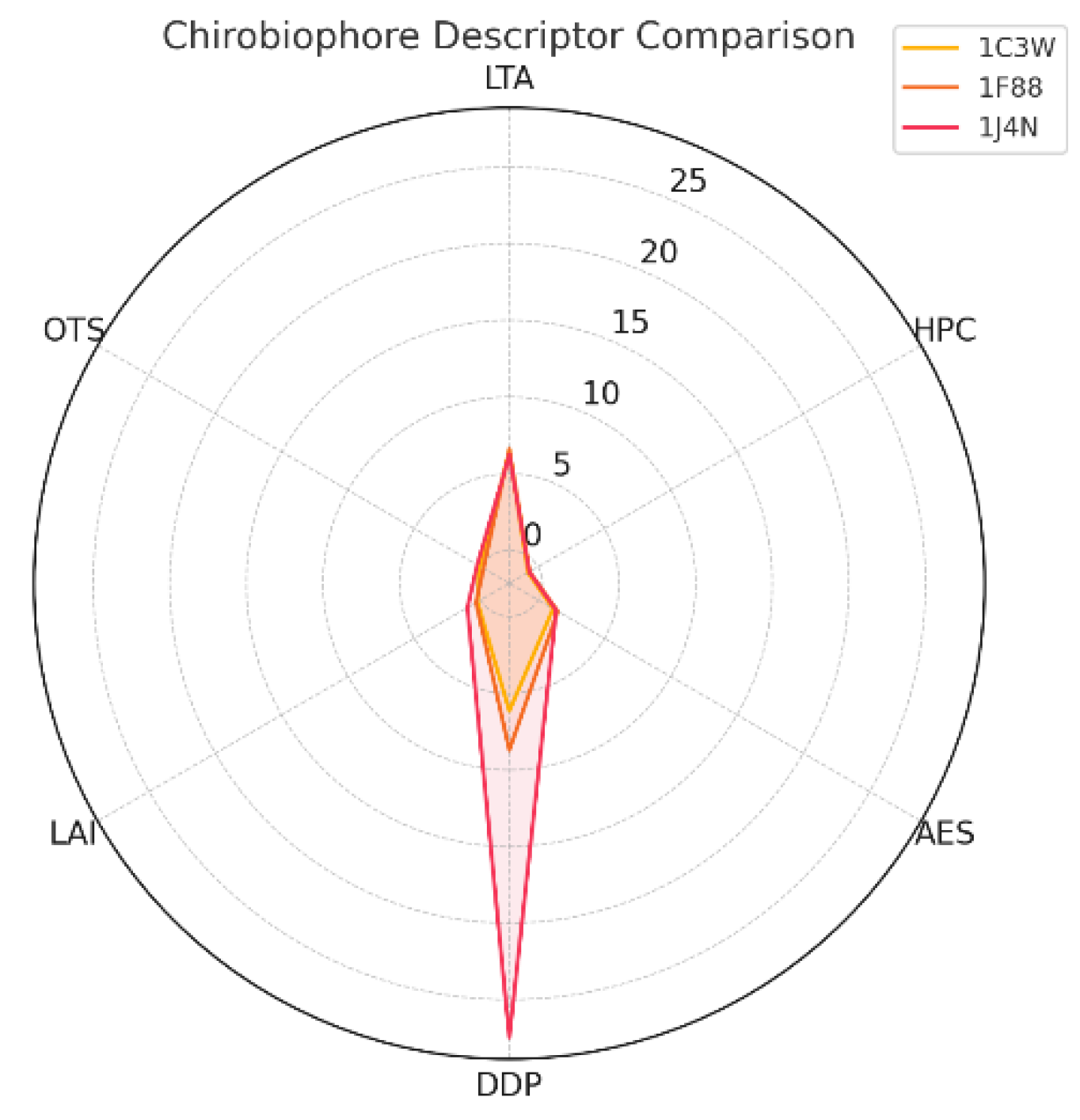
Figure 2.
The radar plot for the GPCR group (2RH1, 3ODU, 4DKL) shows how each protein expresses chirality across the six Chirobiophore descriptors. 3ODU stands out with extremely high DDP and LAI. 2RH1 has a balanced but elevated chirality profile. 4DKL exhibits the lowest DDP and a negative LAI, indicating a slightly lower-leaflet bias. Radar plot of Chirobiophore descriptors for [protein group]. All six descriptors (LTA, HPC, AES, DDP, LAI, OTS) are shown after z-score standardization (mean = 0, standard deviation = 1) across the analyzed dataset, allowing direct visual comparison of relative descriptor magnitudes. All axes are dimensionless and comparable by construction.
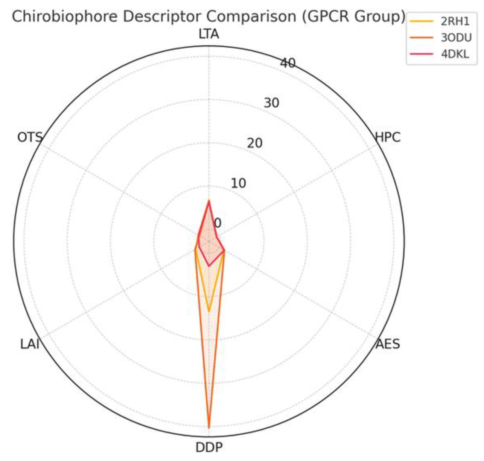
Figure 3.
The radar plot for the complex membrane protein group (2A79, 1C17, 1OTS).
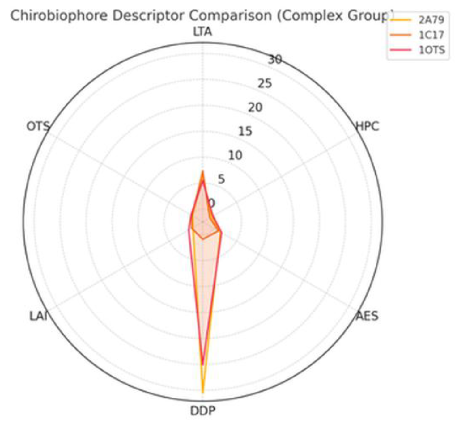
Figure 4.
The radar plot compares all three groups of membrane proteins across the six Chi-robiophore descriptors: Canonical proteins (1C3W, 1F88, 1J4N) show relatively balanced chirality profiles with modest embedding asymmetries. GPCRs (2RH1, 3ODU, 4DKL) are characterized by higher DDP and LAI, reflecting their asymmetric interaction with the membrane. Structurally complex proteins (2A79, 1C17, 1OTS) exhibit the most diverse profiles. Notably, 1C17 leads in LTA and HPC, but is nearly symmetric in embedding, while 1OTS has the highest AES, indicating local geometric disorder. Radar plot of Chirobiophore descriptors for [protein group]. All six descriptors (LTA, HPC, AES, DDP, LAI, OTS) are shown after z-score standardization (mean = 0, standard deviation = 1) across the analyzed dataset, allowing direct visual comparison of relative descriptor magnitudes. All axes are dimensionless and comparable by construction.
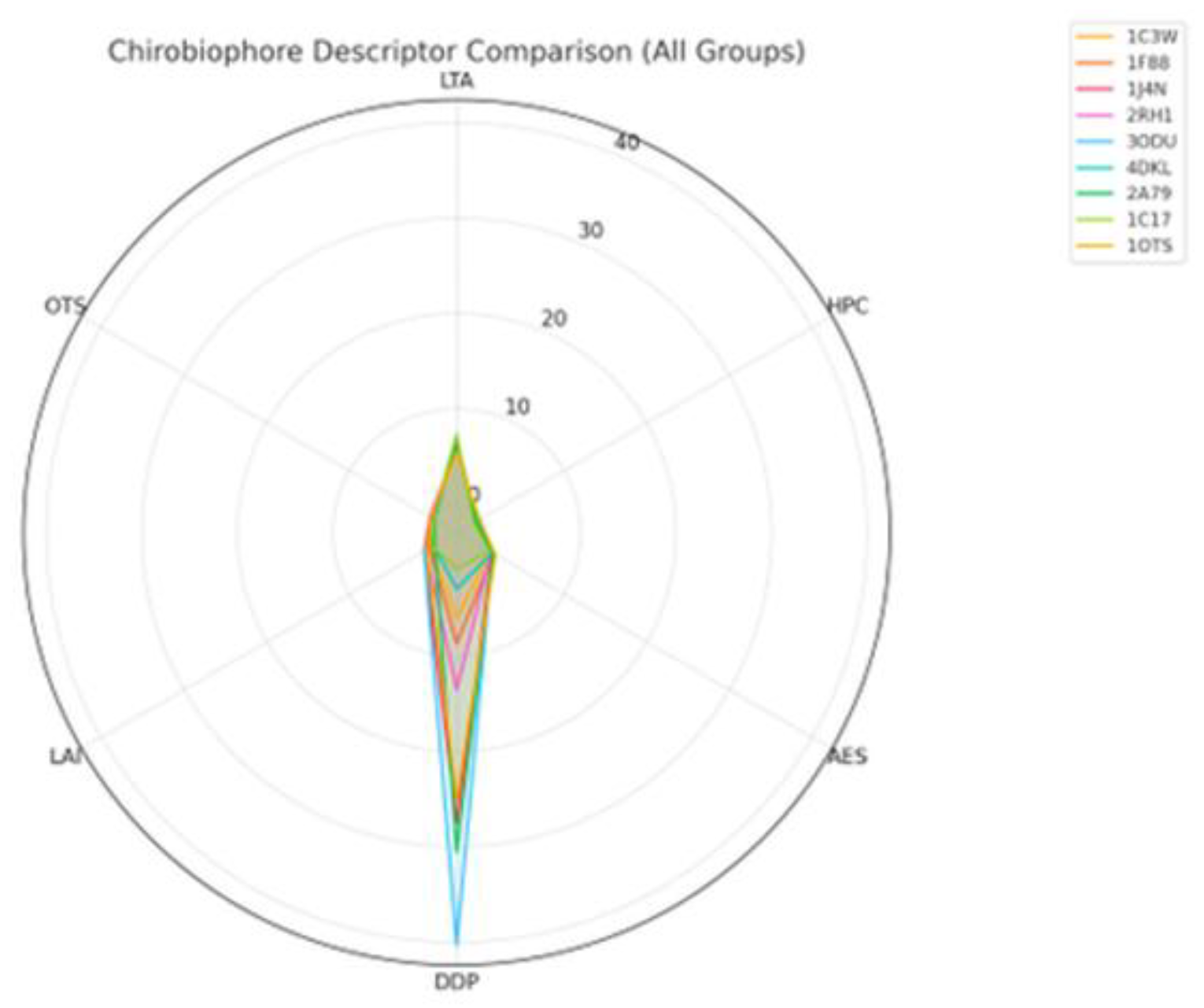
Figure 5.
Chirobiophore group statistics.
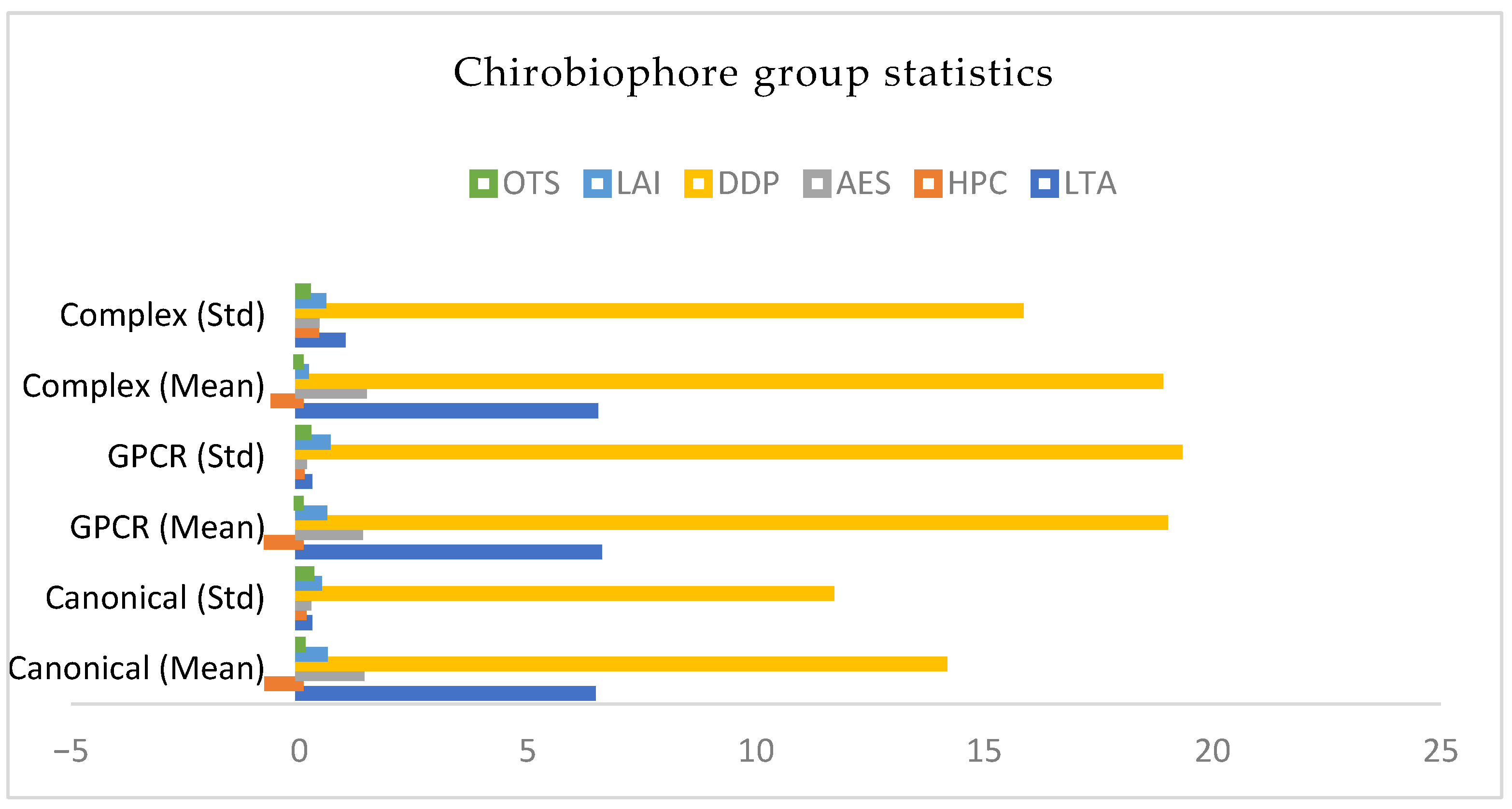
Figure 6.
Clustering groups 3ODU, 2RH1, and 2A79 closely, highlighting their shared asymmetric embeddings and twist patterns. 1C17 is most distinct due to its extreme LTA and HPC. Canonical proteins (1C3W, 1F88, 1J4N) cluster nearby but with some divergence based on DDP.
Figure 6.
Clustering groups 3ODU, 2RH1, and 2A79 closely, highlighting their shared asymmetric embeddings and twist patterns. 1C17 is most distinct due to its extreme LTA and HPC. Canonical proteins (1C3W, 1F88, 1J4N) cluster nearby but with some divergence based on DDP.
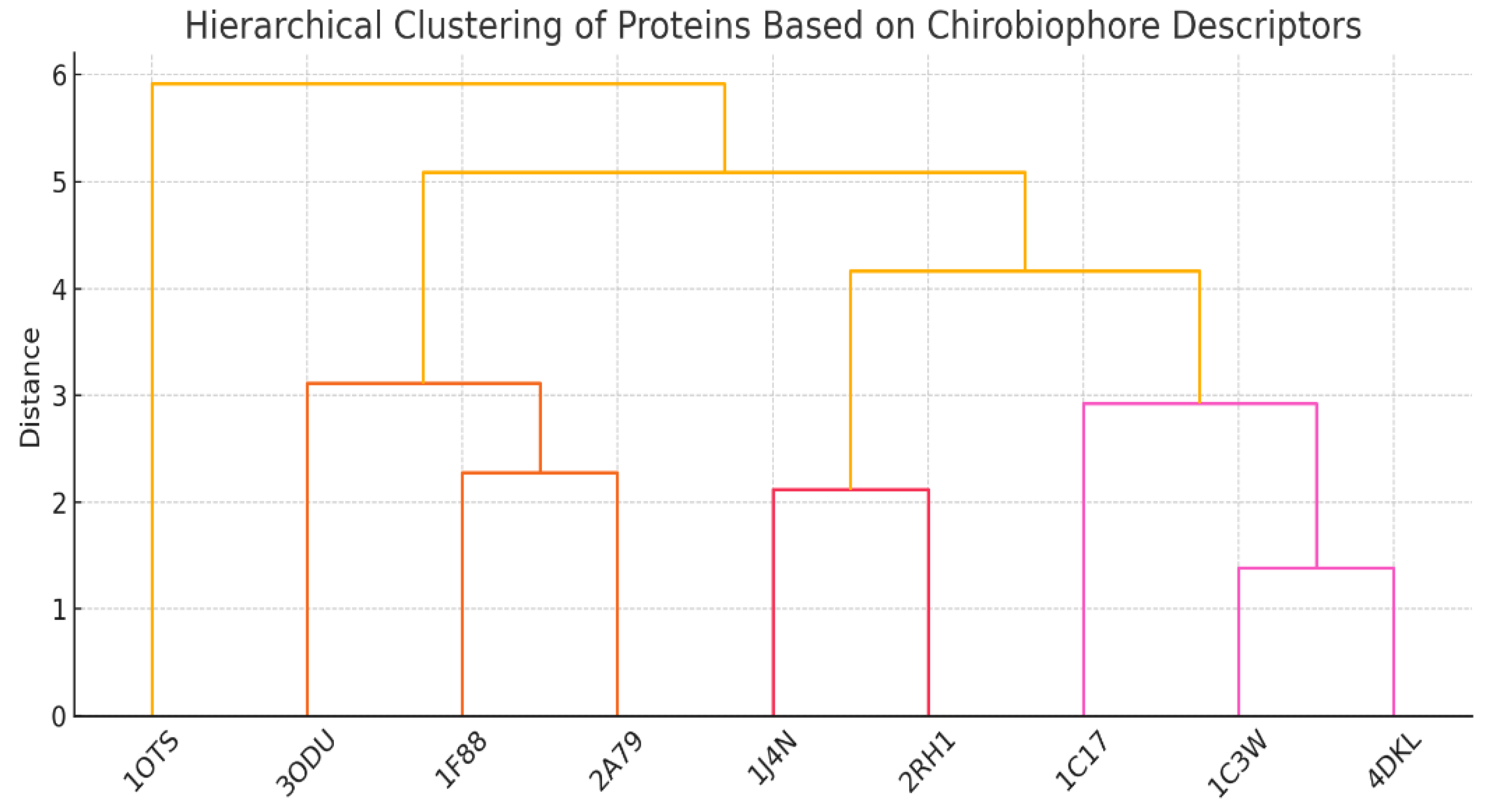
Figure 7.
The heatmap of standardized Chirobiophore descriptors across all 9 proteins. 1C17 shows a substantial positive deviation in LTA and HPC, reflecting tight, regular helicity. 3ODU and 2A79 have elevated DDP, aligning with their deep asymmetric membrane embedding 1OTS stands out with the highest AES, indicating severe local packing asymmetryGPCRs tend to be elevated in LAI (upper leaflet bias), while 1C17 and 1F88 hover near balance.
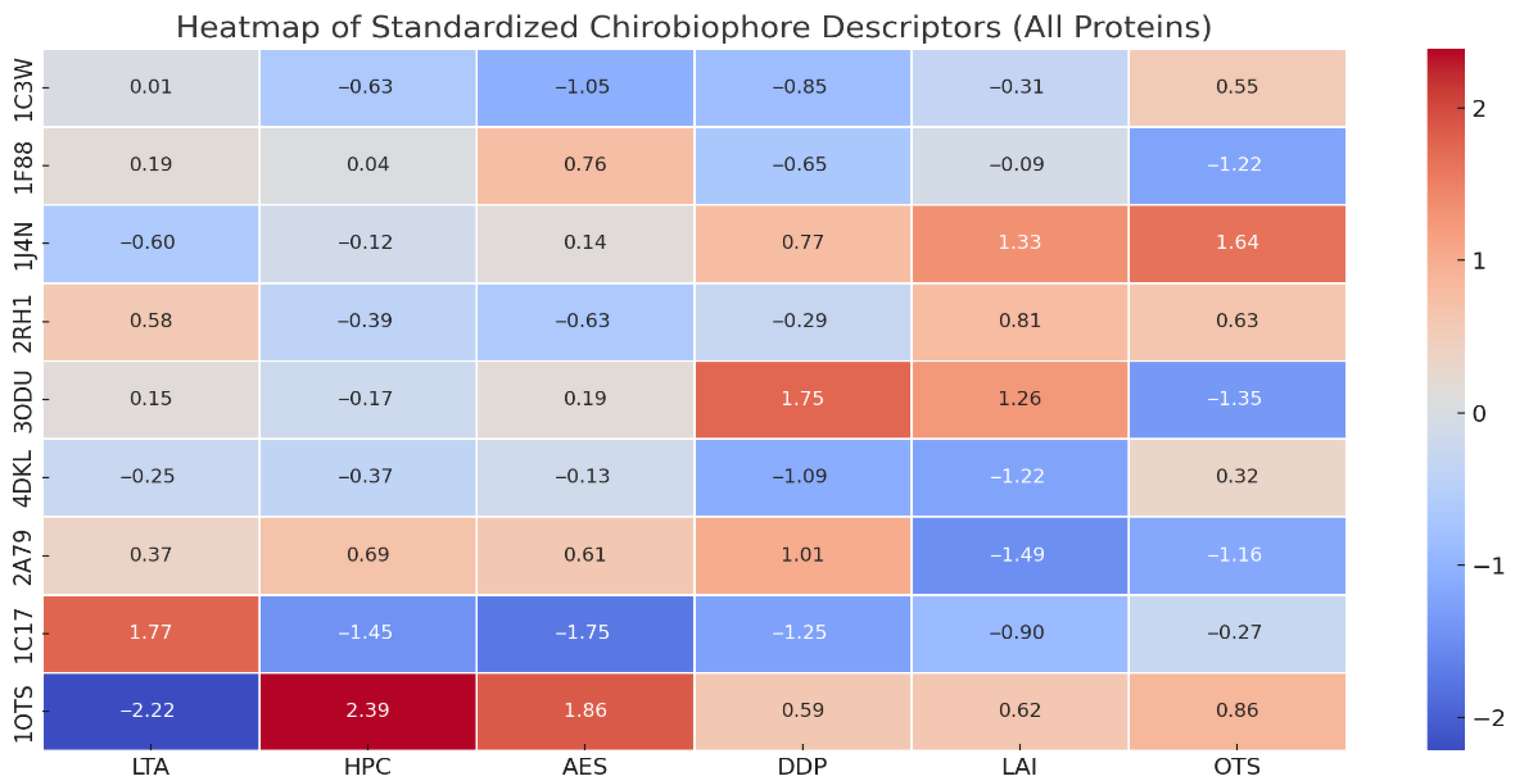
Figure 8.
Chirobiophore manifold representation. A 3D PCA-based manifold representation of the Chirobiophore space: Each point represents a protein’s full chirality vector projected into 3D. This serves as a “local chart” of the 6D manifold—akin to slicing the Riemannian space for visualization. Clustering (e.g., canonical group), branching (e.g., 1C17 diverging), and gradient flow across descriptors, such as DDP and OTS, can be observed.
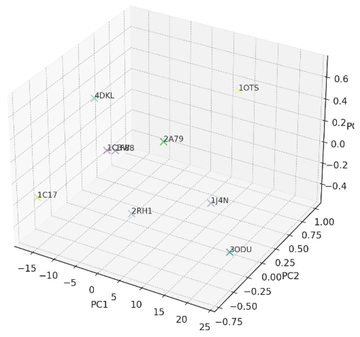
Figure 9.
Smooth manifold mesh fitted through the Chirobiophore space. The surface represents a continuous interpolation of the chirality vectors. Proteins are defined as discrete points, positioned according to PCA in this chart. The curvature and slope of the surface suggest gradients in chirality behavior—analogous to a flow on a Riemannian manifold [43]. Low-dimensional manifold representation of the Chirobiophore space derived from PCA projection of standardized descriptor vectors. The surface represents a smooth interpolation of the descriptor space and is intended for qualitative visualization of structural relationships rather than quantitative distance measurement.
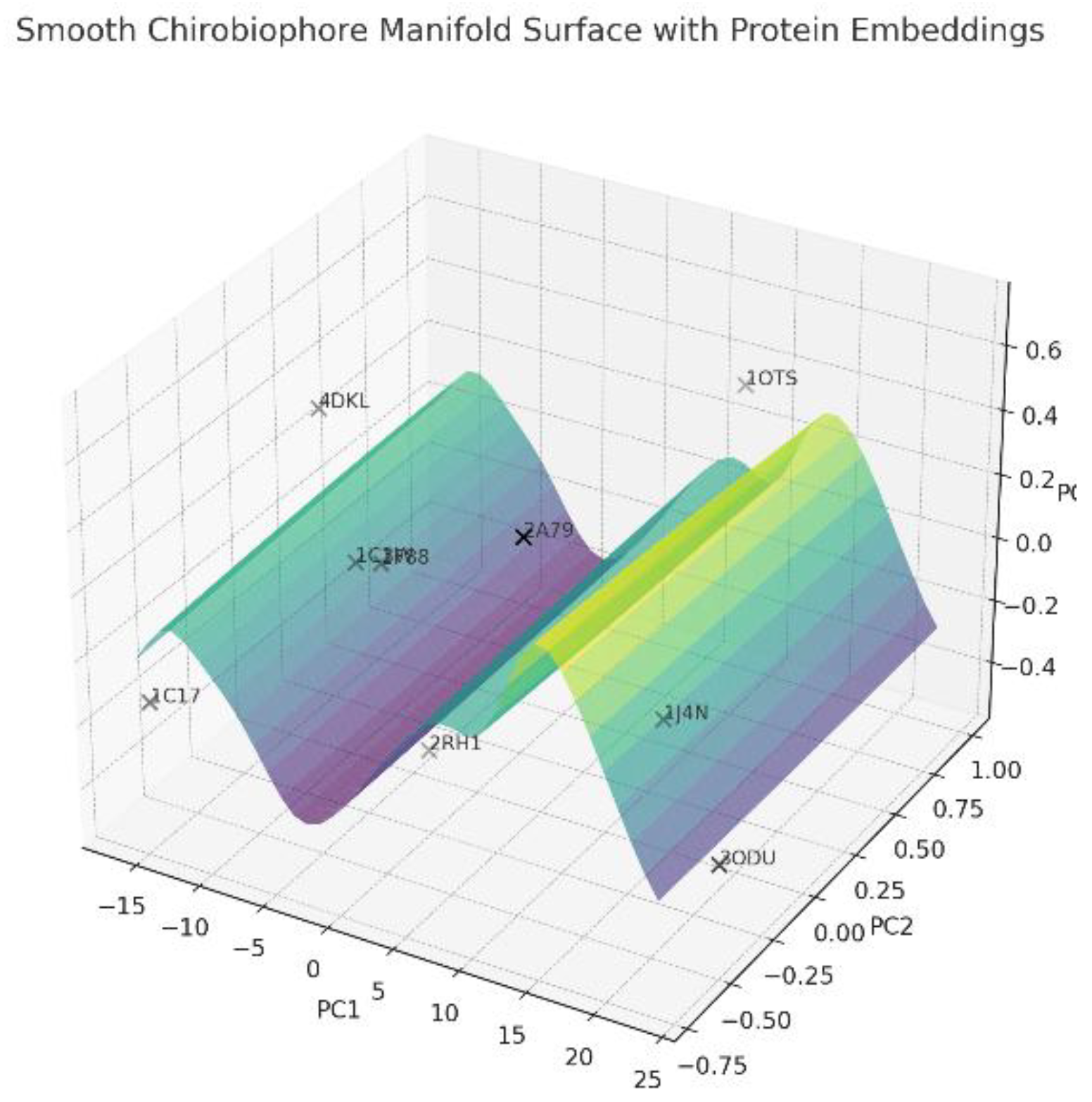
Figure 10.
The gradient flow field for the descriptor ∇DDP (Directional Density Profile): Arrows indicate how proteins might “flow” across the Chirobiophore manifold if DDP increases or decreases. The color map represents DDP intensity over the PC1–PC2 projection. Evolutionary or structural changes can be modeled as paths along these vector fields.
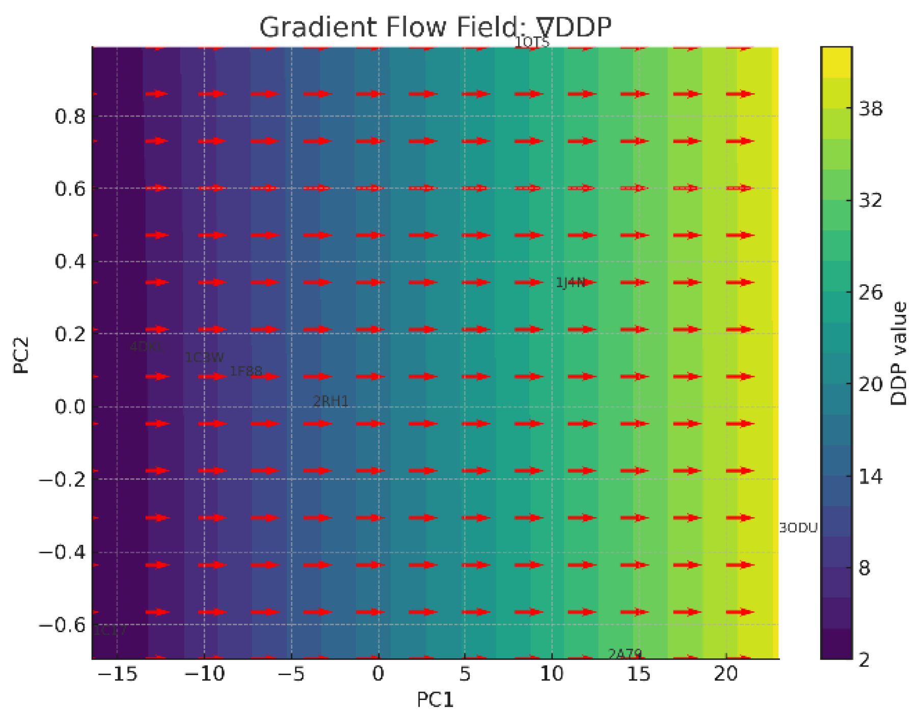
Figure 11.
Gradient fields representation. Interpretation of Gradient Flow Fields (∇Descriptors): Each plot illustrates how a specific descriptor (e.g., LTA, DDP) varies across the 2D PCA embedding of all proteins. Arrows represent the local gradient direction and magnitude—that is, how the descriptor value changes in nearby regions. Collectively, these gradients provide a view of potential evolutionary, conformational, or functional “flows” in chirality space.
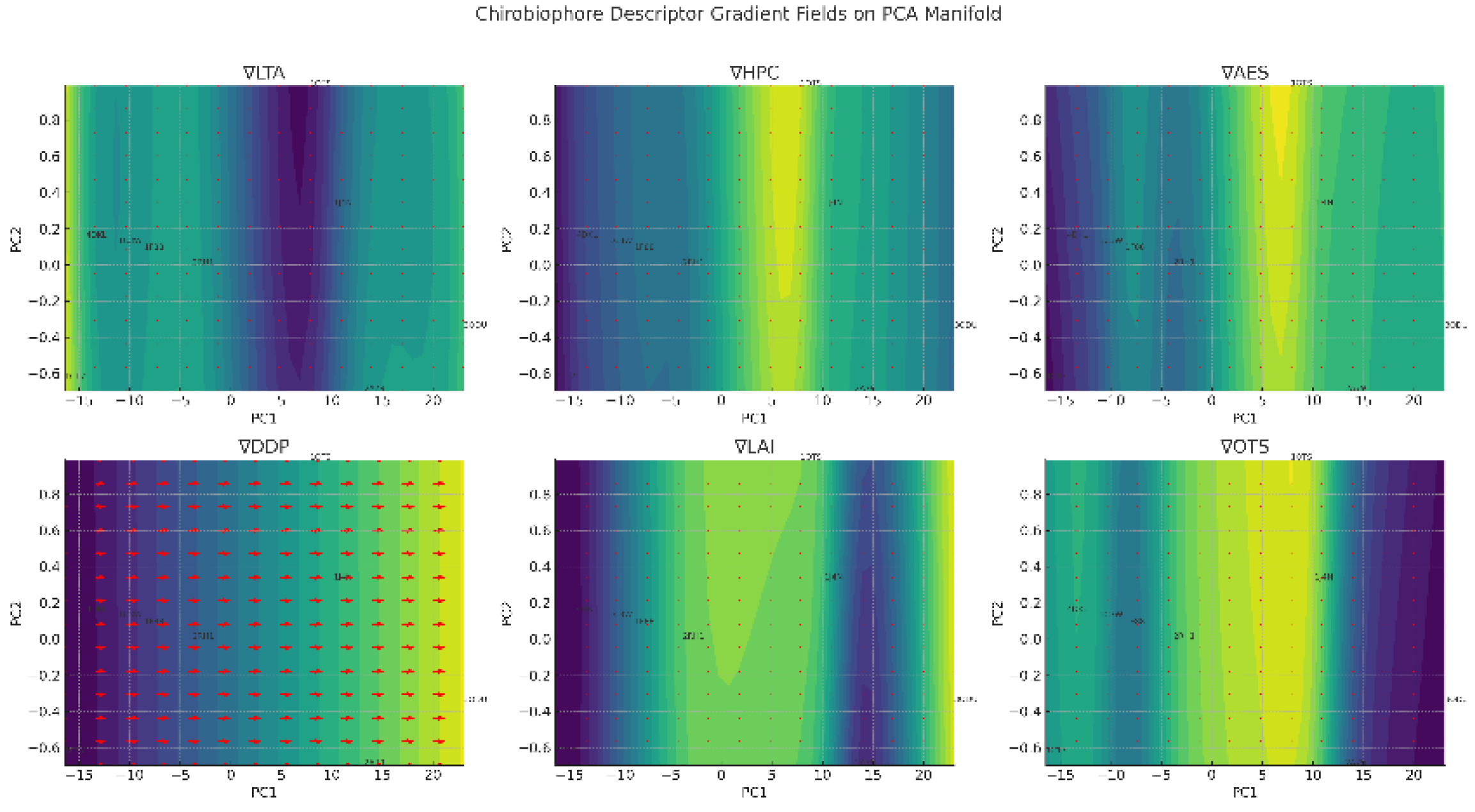
Table 1.
Descriptors summarized.
| Descriptor | Type | Measures | Application |
| CPS | Persistence | Lifespan of chiral features | Robustness of asymmetry |
| CGI | Genus | Number of chirality domains | Complexity of chiral topology |
| CVF | Curl | Twist/swirl of the chirality field | Membrane rotation bias |
| CEI | Linking | Intertwining of chirality paths | Folded structures, channels |
| TCC | Entropy | Predictability of chirality transitions | Functional modularity |
Table 2.
Protein type and chirobiophore descriptors results.
| Protein Type | PDB | LTA | HPC | AES | DDP | LAI | OTS |
| Canonicalα-helical membrane proteins | 1c3w Bacteriorhodopsin | 6.47 | −0.75 | 1.14 | 6.16 | 0.25 | 0.08 |
| 1f88 Rhodopsin | 6.55 | −0.63 | 1.49 | 8.71 | 0.35 | −0.21 | |
| 1j4n Aquaporin-1 | 6.19 | −0.66 | 1.37 | 27.46 | 1.00 | 0.26 | |
| G protein-coupled receptors | 2rh1 β2-Adrenergic Receptor | 6.73 | −0.71 | 1.22 | 13.52 | 0.76 | 0.09 |
| 3odu CXCR$ chemokine receptor | 6.53 | −0.67 | 1.38 | 40.33 | −0.97 | −0.23 | |
| 4dkl Miu-opioid receptor | 6.35 | −0.70 | 1.32 | 2.99 | −0.16 | 0.04 | |
| Topological complex membrane proteins | 2a79 Voltage-gated potassium channel | 6.63 | −0.51 | 1.46 | 30.52 | −0.29 | −0.20 |
| 1c17 ATP synthase subunit c | 7.27 | −0.90 | 1.01 | 0.89 | −0.02 | −0.05 | |
| 1ots Clc chloradie transporter | 5.45 | −0.21 | 1.70 | 25.10 | 0.67 | 0.13 |
Table 3.
Descriptor values for 1C3W.
| Descriptor | Value | Interpretation |
| LTA (Local Tetrahedral Asymmetry) | 6.47 | Moderate local chirality in atomic geometry |
| HPC (Helical Path Curvature) | −0.75 | Predominantly left-handed torsion pattern |
| AES (Asymmetric Environment Score) | 1.14 | Moderate angular asymmetry in local packing |
| DDP (Directional Density Profile) | 6.16 | Density skewness along the Z-axis reflects bilayer alignment |
| LAI (Leaflet Asymmetry Index) | 0.25 | Slight enrichment in the upper membrane leaflet |
| OTS (Orientation Twist Score) | 0.08 rad | Mild overall helix tilt in the membrane |
Table 4.
Descriptor values for 1F88.
| Descriptor | Value | Interpretation |
| LTA | 6.55 | Local atomic asymmetry is moderate-high |
| HPC | −0.63 | Backbone shows predominantly left-handed torsion |
| AES | 1.49 | Elevated local packing disorder |
| DDP | 8.71 | Pronounced mass asymmetry along the membrane axis |
| LAI | 0.35 | Clear preference toward the upper membrane leaflet |
| OTS | −0.21 rad | Moderate net left-handed twist in membrane helices |
Table 5.
descriptor values for 1J4N.
| Descriptor | Value | Interpretation |
| LTA | 6.19 | Moderate geometric chirality at the atomic level |
| HPC | −0.66 | Consistent left-handed torsional pattern |
| AES | 1.37 | Modest angular asymmetry in local environments |
| DDP | 27.46 | Substantial mass displacement along the Z-axis—highly embedded or tilted |
| LAI | 1.00 | Entirely embedded in the upper leaflet region |
| OTS | 0.26 rad | Noticeable right-handed tilt of transmembrane helices |
Table 6.
descriptor values for 2RH1.
| Descriptor | Value | Interpretation |
| LTA | 6.73 | High atomic-scale chirality |
| HPC | −0.71 | Strong left-handed torsional bias |
| AES | 1.22 | Moderate local packing asymmetry |
| DDP | 13.52 | Clear structural tilt or directional embedding |
| LAI | 0.76 | Strong upper leaflet preference |
| OTS | 0.09 rad | Mild right-handed membrane twist |
Table 7.
descriptor values for 3ODU.
| Descriptor | Value | Interpretation |
| LTA | 6.53 | Moderate-high geometric asymmetry |
| HPC | −0.67 | Predominantly left-handed helix alignment |
| AES | 1.38 | Noticeable packing disorder |
| DDP | 40.33 | Extremely asymmetric embedding along the Z-axis |
| LAI | 0.97 | Nearly all structure lies in the upper leaflet. |
| OTS | −0.23 rad | Left-handed membrane twist orientation |
Table 8.
descriptor values for 3ODU.
| Descriptor | Value | Interpretation |
| LTA | 6.35 | Moderate local torsional asymmetry |
| HPC | −0.70 | Strong left-handed helical coherence |
| AES | 1.32 | Moderate environmental asymmetry |
| DDP | 2.99 | Relatively symmetric depth embedding |
| LAI | −0.16 | Slight lower leaflet embedding bias |
| OTS | 0.04 rad | Near-neutral twist orientation |
Table 9.
.
| Descriptor. | Value | Interpretation |
| LTA | 6.63 | Strong atomic asymmetry |
| HPC | −0.51 | Moderate left-handed backbone torsion |
| AES | 1.46 | Noticeable packing irregularity |
| DDP | 30.52 | Deep asymmetric embedding along Z-axis |
| LAI | −0.29 | Skewed toward the lower leaflet |
| OTS | −0.20 rad | Left-handed membrane twist |
Table 10.
descriptor values for 1C17.
| Descriptor | Value | Interpretation |
| LTA | 7.27 | Highest chirality at the atomic level among all |
| HPC | −0.90 | Very strong left-handed helical bias |
| AES | 1.01 | Relatively symmetric local packing |
| DDP | 0.89 | Near-symmetric depth distribution |
| LAI | −0.02 | Almost perfectly balanced leaflet alignment |
| OTS | −0.05 rad | Neutral to weak left-handed twist |
Table 11.
descriptor values for 1OTS.
| Descriptor | Value | Interpretation |
| LTA | 5.45 | Lowest local atomic asymmetry among all |
| HPC | −0.21 | Weak torsional coherence |
| AES | 1.70 | Highest packing asymmetry, very irregular |
| DDP | 25.10 | Strong structural bias along Z |
| LAI | 0.67 | Embedded predominantly in upper leaflet |
| OTS | 0.13 rad | Mild right-handed twist bias |
Table 12.
PCA analysis.
| Descriptor | PC1 (Global Chirality) | PC2 (Membrane Orientation Bias) |
| LTA | −0.50 | +0.20 |
| HPC | +0.51 | +0.14 |
| AES | +0.50 | +0.26 |
| DDP | +0.38 | +0.28 |
| LAI | +0.28 | −0.37 |
| OTS | +0.12 | −0.81 (dominant) |
Table 13.
Relating Chirobiophore Descriptors to Tissular Indices.
| Chirobiophore Descriptor | Biophysical Meaning | Potential Tissular Index | Biological Correlate |
| LTA (Local Tetrahedral Asymmetry) | Atomic-scale chirality in geometry | Planar cell polarity (PCP) indices | Left-right biased cell elongation, neural tube closure |
| HPC (Helical Path Coherence) | Helical regularity along backbone | Orientation vector fields in epithelia | Hair cell stereocilia alignment, gut tube spirals |
| AES (Packing Asymmetry) | Irregularity of atomic environments | Tissue anisotropy tensors | Myocardial fiber misalignment, ECM polarization |
| DDP (Directional Density Profile) | Z-axis skew (e.g., depth asymmetry) | Basal–apical polarity index, tissue skew index | Epithelial invagination, somite slanting |
| LAI (Leaflet Asymmetry Index) | Membrane bilayer bias | Apical surface area asymmetry, lumen eccentricity | Left-right biased organ budding (e.g., lung lobes) |
| OTS (Orientation Twist Score) | Helical tilt or twist | Rotational tissue morphogenesis, spiral index | Gut coiling, cardiac looping, limb torsion |
Table 14.
Indexes used in the study.
| Index | Description |
| MECI (Membrane Embedding Contrast Index) | Highlights depth asymmetry relative to helical twist. |
| TMOI (Transmembrane Orientation Index) | Describes how helices orient or tilt in membrane space. |
| HRS (Helical Regularity Score) | Reflects the consistency of torsional helical geometry. |
| ABAI (Apicobasal Asymmetry Index) | Combines membrane depth and leaflet bias to model apical-basal asymmetry. |
Table 15.
Tisular indices.
| Index | Formula | Biological Interpretation |
| PSI (Polarity Skew Index) | PSI = 0.6⋅DDP~ + 0.4⋅LAI~\text{PSI} = 0.6 \cdot \tilde{\text{DDP}} + 0.4 \cdot \tilde{\text{LAI}}PSI = 0.6⋅DDP~ + 0.4⋅LAI~ | Membrane asymmetry and leaflet bias |
| RBI (Rotational Bias Index) | RBI = 0.7⋅OTS~ + 0.3⋅HPC~\text{RBI} = 0.7 \cdot \tilde{\text{OTS}} + 0.3 \cdot \tilde{\text{HPC}}RBI = 0.7⋅OTS~ + 0.3⋅HPC~ | Helical twist + torsional coherence |
| PDI (Packing Disparity Index) | PDI = 0.5⋅AES~ + 0.5⋅LTA~\text{PDI} = 0.5 \cdot \tilde{\text{AES}} + 0.5 \cdot \tilde{\text{LTA}}PDI = 0.5⋅AES~ + 0.5⋅LTA~ | Local irregularity + geometric asymmetry |
| MECI (Membrane Embedding Contrast Index) | MECI = 0.5⋅(DDP~ − OTS~)\text{MECI} = 0.5 \cdot (\tilde{\text{DDP}} − \tilde{\text{OTS}})MECI = 0.5⋅(DDP~ − OTS~) | Z-depth skew minus twist |
| TMOI (Transmembrane Orientation Index) | TMOI = 0.6⋅OTS~ + 0.4⋅LAI~\text{TMOI} = 0.6 \cdot \tilde{\text{OTS}} + 0.4 \cdot \tilde{\text{LAI}}TMOI = 0.6⋅OTS~ + 0.4⋅LAI~ | Orientation in the membrane bilayer |
| HRS (Helical Regularity Score) | HRS = 0.5⋅HPC~ + 0.5⋅LTA~\text{HRS} = 0.5 \cdot \tilde{\text{HPC}} + 0.5 \cdot \tilde{\text{LTA}}HRS = 0.5⋅HPC~ + 0.5⋅LTA~ | Backbone coherence + chirality |
| ABAI (Apicobasal Asymmetry Index) | ABAI = 0.5⋅DDP~ + 0.5⋅LAI~\text{ABAI} = 0.5 \cdot \tilde{\text{DDP}} + 0.5 \cdot \tilde{\text{LAI}}ABAI = 0.5⋅DDP~ + 0.5⋅LAI~ | Depth and leaflet asymmetry |
| TPI (Tissue Polarity Index) | TPI = OTS~ + LAI~\text{TPI} = \tilde{\text{OTS}} + \tilde{\text{LAI}}TPI = OTS~ + LAI~ | Global polarity vector |
| MCI (Morphogenetic Complexity Index) | MCI = AES~ + LTA~ + DDP~\text{MCI} = \tilde{\text{AES}} + \tilde{\text{LTA}} + \tilde{\text{DDP}}MCI = AES~ + LTA~ + DDP~ | Structural complexity and irregularity |
| FCI (Functional Chirality Index) | FCI = HPC~ + OTS~ + AES~\text{FCI} = \tilde{\text{HPC}} + \tilde{\text{OTS}} + \tilde{\text{AES}}FCI = HPC~ + OTS~ + AES~ | Combined handedness and orientation |
| API (Anisotropy-Packing Index) | API = LTA~ + AES~ + DDP~\text{API} = \tilde{\text{LTA}} + \tilde{\text{AES}} + \tilde{\text{DDP}}API = LTA~ + AES~ + DDP~ | Spatial anisotropy and density contrast |
Table 16.
Summary of Topological Power.
| Feature | Interpretation |
| Chirality space (ℝ6) | Global comparison of structure |
| Chirality manifold | Realizable structural chirality domain |
| Graph theory model | Local interactions and chirality propagation |
| Fiber bundle structure | Local chirality vectors at every point |
| Topological invariants | Classify chirality patterns (loops, cavities, genus) |
| Persistence & homology | Detect scale-stable chirality features. |
Disclaimer/Publisher’s Note: The statements, opinions and data contained in all publications are solely those of the individual author(s) and contributor(s) and not of MDPI and/or the editor(s). MDPI and/or the editor(s) disclaim responsibility for any injury to people or property resulting from any ideas, methods, instructions or products referred to in the content. |
© 2026 by the authors. Licensee MDPI, Basel, Switzerland. This article is an open access article distributed under the terms and conditions of the Creative Commons Attribution (CC BY) license (http://creativecommons.org/licenses/by/4.0/).
Copyright: This open access article is published under a Creative Commons CC BY 4.0 license, which permit the free download, distribution, and reuse, provided that the author and preprint are cited in any reuse.


