Submitted:
12 February 2026
Posted:
12 February 2026
You are already at the latest version
Abstract
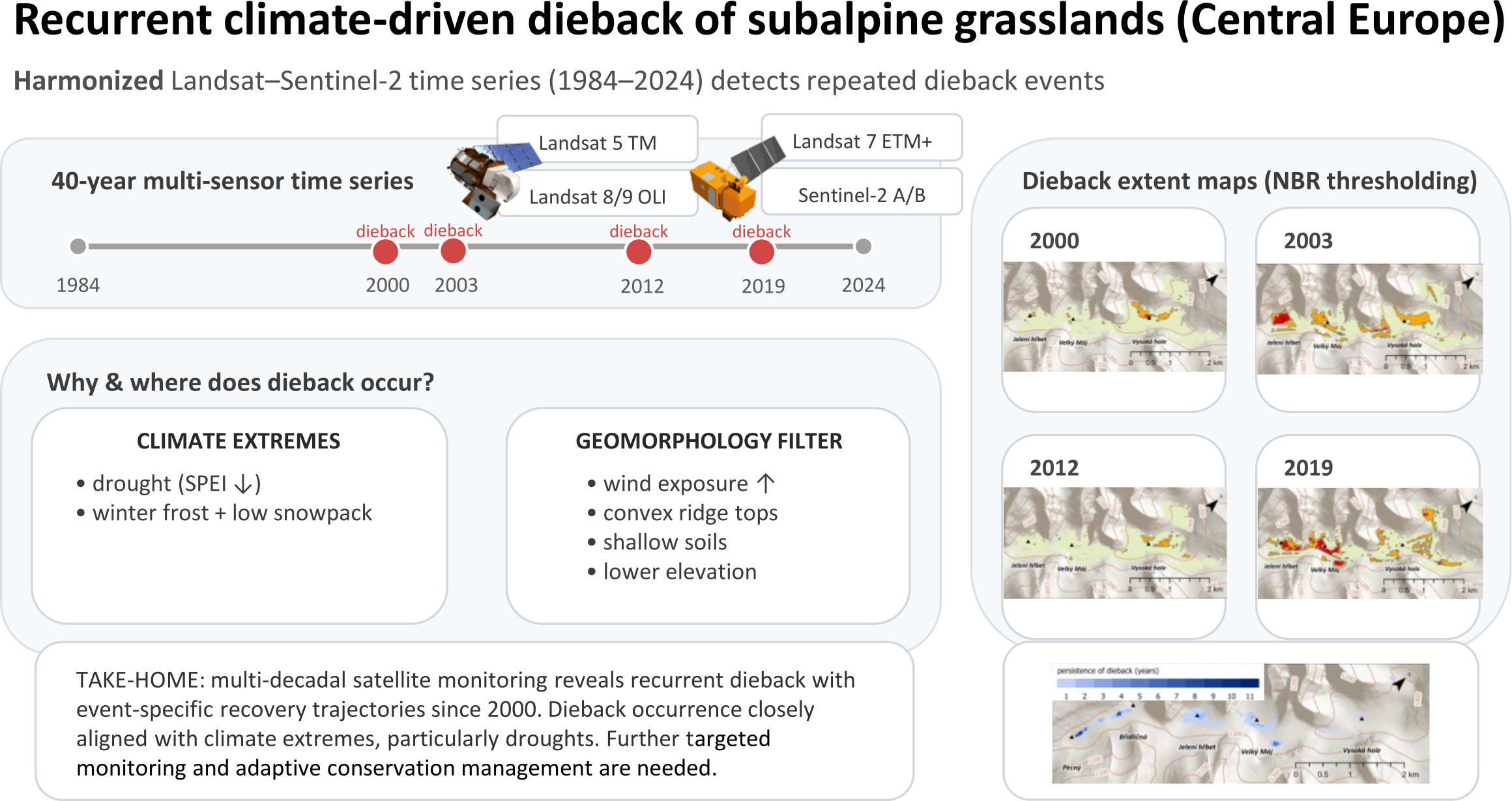
Subalpine grasslands represent highly sensitive ecosystems that are increasingly exposed to climate extremes, yet their long-term disturbance dynamics remain poorly documented. This study investigates climate-driven dieback of subalpine grasslands in Central Europe using a harmonized, multi-decadal satellite time series. We analyzed Landsat (TM, ETM+, OLI, OLI-2) and Sentinel-2 imagery spanning 1984–2024 to detect changes in grassland condition, supported by field-based validation, climatic indices, and geomorphological analysis. Several spectral indices related to non-photosynthetic vegetation were evaluated, with the Normalized Burn Ratio (NBR) showing the highest ability to discriminate dead grassland biomass from live vegetation. Retrospective mapping revealed four distinct dieback events since 2000, comprising two short-term episodes with rapid within-season recovery and two long-term events characterized by persistent degradation and slow regeneration. Dieback timing corresponded closely with climatic extremes, particularly droughts of varying duration, while winter frost under shallow soil conditions likely contributed to long-term damage in some cases. Geomorphological analysis indicated that wind exposure, elevation, and terrain convexity strongly modulate dieback susceptibility, highlighting the importance of fine-scale environmental controls. Our results demonstrate the value of long-term, multi-sensor satellite observations for detecting and interpreting climate-driven disturbances in subalpine grasslands and provide a transferable framework to support monitoring and conservation of mountain ecosystems under ongoing climate change.
Keywords:
subalpine grasslands
; grassland dieback
; climate extremes
; Landsat
; Sentinel-2
; time series analysis
; non-photosynthetic vegetation
; mountain ecosystems
; Central Europe
; geomorphological controls
1. Introduction
Alpine and subalpine ecosystems are among the most vulnerable to global change, primarily due to their limited and fragmented spatial distribution, confinement to higher elevations, and the overall adaptation of mountain species to cool and moist environmental conditions, especially in the temperate zone of Europe [1,2,3]. Particularly dramatic transformations may be observed in subalpine habitats of mid-latitude mountain ranges, such as the Sudetes, where subalpine grasslands form the highest vegetation belt. The ongoing progression of global warming [4] is inducing significant alterations in subalpine ecosystems, most notably triggering an upward shift of the treeline, which is primarily constrained by temperature [1,5]. This, in turn, is already contributing to a decline in the extent of treeless habitats [6,7], along with structural and functional modifications within them. These include the upward movement of species distributions [8], compositional shifts in subalpine communities [9,10,11,12], changes in plant physiology and reproduction [13,14], and variations in nutrient cycling and microbial activity [15,16].
In addition to rising temperatures, climate change is modifying precipitation patterns [17], increasing the frequency, magnitude, and duration of extreme events such as droughts [18], and reducing the accumulation of winter snowpack [19]. Historically, alpine and subalpine ecosystems have not been regularly exposed to drought conditions [20], and the comparatively lower drought resistance of subalpine grasslands may be attributed to their shallower rooting systems relative to forests. As a result, persistent soil moisture deficits may lead to severe water stress, declines in productivity, and potential dieback of grassland vegetation [21]. Additionally, diminished snow depth may lead to more severe soil freezing, increasing the risk of freezing damage to perennial vegetative structures [22,23].
Initially, the effects of reduced snow cover and early snowmelt [24,25,26], as well as extreme droughts [27,28,29], were extensively investigated in alpine and subalpine habitats, typically through manipulative experiments. These experiments have demonstrated that alpine grasslands may suffer severe declines in vitality, even leading to dieback [30].
Over the past two decades, reports of severe drought events in Central Europe have begun to emerge, underscoring their substantial impact on grassland vegetation. This recent dry period has been assessed as extraordinary in the context of the last two millennia [31]. In the Czech Republic, numerous episodes of early vegetation season (April–June) soil drought have been indicated using soil water balance model SoilClim [32,33], some of those fulfilling the conditions for being labeled as “flash droughts”, causing rapid decrease of soil water content in topsoil layer within only few weeks [34]. A notable reduction in primary productivity across Europe was documented already during the 2003 European heatwave [35]. Significant community composition changes were observed in mountain Nardus grasslands in the Rhön Mountains, Germany [36], following the severe summer droughts of 2015 [37] and 2018–2019 [38]. The impact of the same event on lowland grasslands was assessed via remote sensing in northeastern Germany [39], revealing a substantial increase in the non-photosynthetic fraction of grassland cover, particularly on less productive, sandy soils. The extreme drought of 2022 [40] caused notable dieback of dominant perennial grasses in open sandy grasslands in Hungary [41]. Prior to this, drought-induced dieback was reported in alpine Poa grasslands in Australia in 2007 [42].
Repeated dieback in subalpine grasslands in the Hrubý Jeseník Mountains, Czech Republic, was first reported by local conservation authorities (see Figure 1). Subsequent research focused on assessing vegetation changes associated with dieback [43], evaluating management approaches aimed at accelerating regeneration [44], and investigating historical long-term land-use conditions that may have contributed to the current state of subalpine grassland ecosystems [45].
Remote sensing techniques offer extensive opportunities for monitoring vegetation cover dynamics in both near-real-time and retrospective analyses. This is particularly effective through indicators of non-photosynthetic biomass coupled with change detection methods. Specifically, the non-photosynthetic vegetation fraction (NPV) can be effectively indicated using a variety of spectral vegetation indices, collectively referred to as NPV indices. These have been addressed in numerous studies, many of which employ spectral unmixing methods (either regression-based or in combination with synthetic training data derived from spectral libraries) to differentiate NPV from bare soil and photosynthetic vegetation (PV) fractions [46,47,48,49,50]. Most NPV indices are designed to detect either the presence or absence of chlorophyll, primarily using red, red-edge, and near-infrared (NIR) bands [51,52]; or vegetation water-content deficits, using shortwave infrared (SWIR) bands [53,54]. Notably, a generalized framework for drought monitoring in Central European grasslands using Sentinel-2 time series was proposed by Kowalski et al. [55], building on the previously developed Normalized Difference Fraction Index (NDFI) [39]. Although the applicability of specific NPV indices may vary by site, the studies demonstrate that NPV index-based detection of dead phytomass in grasslands can serve as a robust indicator for examining extreme vegetation changes. Since the NPV/PV fraction ratio is also influenced by phenological cycles characterized by seasonal grassland growth and senescence, utilizing time series of multi- and hyperspectral imagery, rather than single-date images, can greatly enhance our ability to distinguish irreversible changes such as dieback from regular seasonal variability [48,56,57,58].
In this study, we pursued three main scientific objectives:
- To identify the most suitable Non-Photosynthetic Vegetation (NPV) index for detecting dieback in subalpine grasslands of the Hrubý Jeseník Mountains.
- To perform a retrospective analysis using archival satellite imagery to determine the onset and progression of dieback events, their spatial localization and extent, as well as the post-event recovery dynamics of subalpine grasslands.
- To evaluate the influence of climate extremes and geomorphology on the spatiotemporal distribution of dieback events, including the relative contribution of factors to explaining the phenomenon.
2. Materials and Methods
2.1. Study Area
The study area is situated in the southern part of the Hrubý Jeseník Mountains in northeastern Czech Republic. This mountain range represents the second-highest massif in the country and forms part of the Sudetes. The investigated area is restricted to the treeless section of the main mountain ridge, which extends from southwest to northeast and encompasses the highest peaks of the range at an altitude of approximately 1330 to 1491 m above sea level. The location and spatial extent of the study area are shown in Figure 2.
The current treeline in the Hrubý Jeseník Mountains lies at approximately 1,250–1,300 m a.s.l. Above this elevation, the ridge is characterized by convex or plateau-like summits separated by concave saddles. The geological substrate is dominated by metamorphic rocks, primarily phyllites with minor occurrences of metadolerites, locally overlain or intermixed with deluvial sediments (https://mapy.geology.cz/arcgis/rest/services/Pudy/pudni_typy50/MapServer?f=jsapi). Soils across the ridge are strongly acidic (pH in H2O varies from 3.5 to 4 in A horizons) and consist mainly of shallow, skeletal rankers and podzols. Peat bogs occur locally, most notably on the summit plateau of Velký Máj and in some saddle depressions. Soil depth is generally limited, rarely exceeding 40 cm even in saddle areas, and is particularly shallow in the southwestern part of the ridge near Břidličná, where depths of only 4–6 cm have been documented.
Climatic conditions in the study region reflect pronounced recent warming trends caused by the ongoing anthropogenic climate change. According to Dolák et al. [59], mean annual air temperature increased from 1.0 °C during the period 1961–1990 to 2.0 °C, or even 2.2 °C, according to Lipina and Šustková [60] in 1991–2020. Warming has been more pronounced during summer than in the winter. Long-term mean annual precipitation (1991–2020) ranges from 1,180 mm at 1,300–1,400 m a.s.l. to 1,254 mm above 1,400 m a.s.l.
Vegetation above the upper treeline is dominated by three native habitat types. Siliceous short subalpine grasslands, habitat type 6150 in Natura 2000 classification, occur on flat mountain tops in climatically most extreme conditions. They are entirely dominated by three grass species: Avenella flexuosa, Festuca supina and Nardus stricta. The short subalpine grasslands are prone to sudden dieback and therefore subject of the present study. Subalpine tall grasslands, part of the habitat type 6430, are dominated by grasses Calamagrostis villosa and Luzula luzuloides, less frequently by Luzula sylvatica. Alpine dwarf-shrub vegetation, part of the habitat type 4060, is dominated by Calluna vulgaris, Vaccinium myrtillus and V. vitis-idaea. Parts of the ridge are additionally occupied by stands of the non-native dwarf pine Pinus mugo, which are currently being removed under conservation management. A fine-scale mosaic of other vegetation types is present, including raised bogs, rocky outcrops and screes, springs, tall-forb and fern communities in depressions, and occasional sparse tree cover [61]. The entire area has been protected as part of the Jeseníky Landscape Protected Area, Praděd National Nature Reserve and Site of Community Importance.
2.2. Climate Data
Climatological variables relevant to the study area, including mean daily air temperature and the Standardized Precipitation Evapotranspiration Index (SPEI), were extracted for the Hrubý Jeseník region from gridded datasets of the SoilClim soil water balance model in horizontal resolution of 500 m [33,62] whose calculations use in-situ measurements from the Czech Hydrometeorological Institute (CHMI).
Mean daily temperature was used to determine the onset of the growing season, defined as the first day of a five-day period with mean temperature exceeding 5 °C [63]. This definition enabled alignment and comparison of seasonal index trajectories among years and dieback episodes. Drought conditions were characterized using SPEI computed over 3-, 6-, and 12-month accumulation windows (SPEI-3, SPEI-6, and SPEI-12); in this study, declines below −1 were considered indicative of moderate or severe drought. These indices were used to assess the temporal correspondence between water balance deficits and observed dieback events.
2.3. Construction of a Harmonized Multi-Sensor Surface Reflectance Time Series (1984–2024)
To quantify the onset, extent, and temporal dynamics of subalpine grassland dieback, we constructed a harmonized multi-decadal time series of multispectral satellite imagery from Landsat (TM, ETM+, OLI, OLI-2) and Sentinel-2 (MSI A/B) surface reflectance products covering the period 1984–2024. These missions provide long-term temporal continuity combined with spatial resolutions suitable for retrospective monitoring of the spatially limited treeless zone of the Hrubý Jeseník Mountains.
We generated a spectrally harmonized four-band dataset (Red, NIR, SWIR1, SWIR2) by combining (i) analysis-ready surface reflectance (SR) collections with per-pixel quality screening and (ii) cross-sensor spectral harmonization to a common reference sensor. Landsat SR data were obtained from the USGS Landsat Collection 2 Level-2 SR products, and Sentinel-2 SR data were obtained from the COPERNICUS/S2_SR_HARMONIZED collection in Google Earth Engine (GEE). Spectral harmonization followed the “virtual constellation” concept of NASA’s Harmonized Landsat and Sentinel-2 (HLS) framework, which aims to make multi-sensor observations directly comparable by reducing systematic differences caused by sensor-specific bandpasses and processing chains [64,65]. Unlike standard HLS products, which are distributed on a common 30 m grid and limited to the Sentinel-2 era, our implementation adopted HLS-consistent spectral harmonization while preserving each sensor’s native spatial resolution and acquisition metadata for subsequent analyses and exports.
All image collections were filtered to the study area and restricted to the vegetation season (1 May–30 September). Scenes with excessive cloudiness were excluded using scene-level cloud metadata, applying a maximum cloud cover threshold of 30%.
Digital numbers were converted to unitless surface reflectance values prior to masking and harmonization. Landsat Collection 2 Level-2 SR was scaled using the USGS-provided factor and offset [66]:
ρ = (DN × 0.0000275) − 0.2
Sentinel-2 SR bands in the COPERNICUS/S2_SR_HARMONIZED collection are scaled by 10,000, and reflectance was obtained as:
ρ = DN / 10,000
Clouds, cloud shadows, cirrus, and sensor artefacts were masked using the quality assurance layers provided with each product. For Landsat, masking relied on the QA_PIXEL and QA_RADSAT bands, while for Sentinel-2, QA60 and the Scene Classification Layer (SCL) were used.
All reflectance measurements were harmonized to an OLI-equivalent spectral reference, with Landsat 8/9 used as the reference sensor, consistent with HLS practice where OLI bandpasses serve as the baseline for MSI adjustments. All harmonization transformations were applied after conversion to physical surface reflectance units.
For Sentinel-2 MSI, we applied the official HLS bandpass adjustment (SBAF-style) linear transformation:
where the coefficients aλ and bλ are band-specific, provided separately for Sentinel-2A and Sentinel-2B, and derived from synthetic OLI and MSI reflectances generated by convolving hyperspectral (Hyperion) spectra with sensor spectral response functions [65].
ρλOLI = aλρλMSI + bλ
To reduce discontinuities between Landsat 7 ETM+ and Landsat 8/9 OLI within the long-term time series, we applied published ordinary least squares (OLS) cross-sensor transformation functions for surface reflectance [67]. Landsat 5 TM reflectance was transformed using the same correction coefficients as ETM+, as these sensors are spectrally similar in the VNIR–SWIR region.
Outputs were produced at each sensor’s native surface reflectance pixel size: Landsat reflective bands at 30 m; Sentinel-2 reflective bands at 20 m: upscaled Red, SWIR1, SWIR2, and NIR using band B8A, consistent with the HLS configuration. Each processed acquisition was clipped to the area of interest and exported as a per-date multiband GeoTIFF containing the harmonized four-band reflectance stack (Red, NIR, SWIR1, SWIR2).
All preprocessing was implemented in the Google Earth Engine Code Editor (https://code.earthengine.google.com). The GEE JavaScript code developed for this workflow, is available via GitHub (https://github.com/olkachalova/subalpine_diebacks). The final dataset comprised 214 analysis-ready, harmonized four-band images spanning August 1984 to September 2024.
2.4. Selection, Validation, and Thresholding of the Optimal NPV Index
Among the large number of spectral indices proposed for detecting non-photosynthetic vegetation (NPV) [68,69], we restricted the candidate set to indices that are cross-sensor compatible, i.e., computable using bands available across Landsat 5–9 and Sentinel-2: red, near-infrared (NIR), shortwave infrared 1 (SWIR1), and shortwave infrared 2 (SWIR2). The final set of candidate indices is listed in Table 1.
To validate the performance of the candidate indices, field reference data were collected in July 2022. Homogeneous polygons representing four land cover classes were delineated: (1) dead grassland; (2) semi-open, windswept grasslands dominated by Avenella flexuosa; (3) dense grasslands dominated by Festuca supina and/or Nardus stricta; and (4) non-vegetated surfaces (screes, trails, rocks, built-up features, and recently removed vegetation under experimental management). Validation polygons were digitized using GPS, each with a minimum size of 20 × 20 m (corresponding to the Sentinel-2 SWIR spatial resolution) and located at sufficient distance from neighboring vegetation types to minimize mixed-pixel effects. Non-vegetated areas were digitized using RGB orthophotos.
Validation polygons were subsequently converted to points according to a common Sentinel-2/Landsat computational grid in 10 m resolution, which was used to extract pixel values from the images. In total, 807 validation points were generated; their spatial distribution is shown in Figure 2.
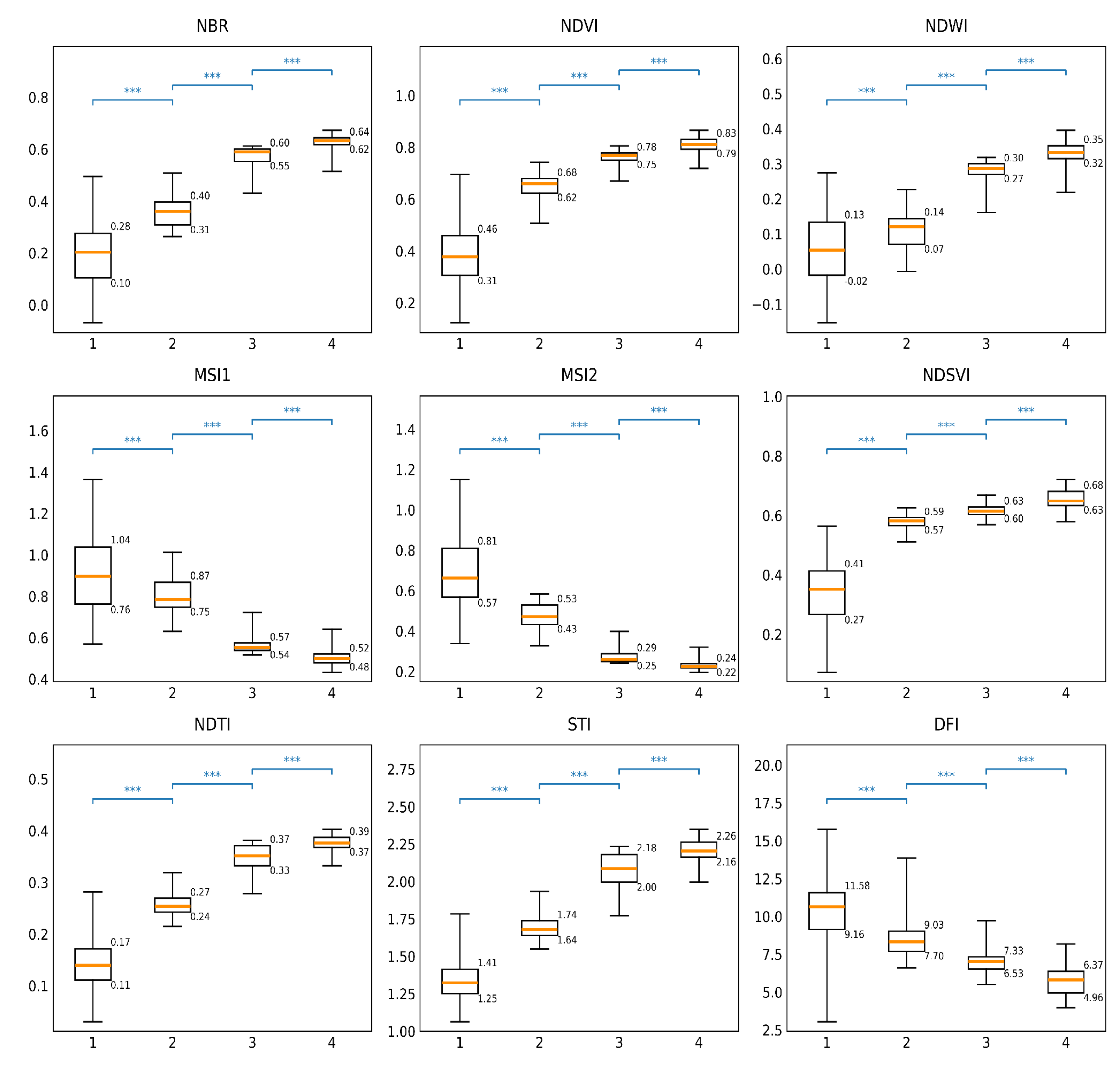
For validation, NPV index values were calculated from the harmonized Sentinel-2 image acquired on 19 July 2022 and the Landsat 9 image acquired on 21 July 2022, representing the closest available dates to the field survey. Index distributions were compared among land cover classes using analysis of variance (ANOVA) and Cohen’s d effect sizes. Given the large sample size, effect sizes were used to assess practical separability among classes. The index that most strongly separated dead grassland from windswept healthy grassland was selected as the primary metric for retrospective dieback mapping, as both classes are characterized by relatively low index values.
Boxplots illustrating the performance of individual NPV indices in distinguishing dead grasslands from other land cover types are shown in Figure 3. Overall, all nine tested indices demonstrated statistically significant separation among the land cover classes. However, the Normalized Burn Ratio (NBR) showed the highest Cohen’s d values for separating dead grassland from windswept grassland (Table 2) and was therefore selected for historical grassland dieback detection.
Considering that some areas affected by the 2019 dieback had already initiated regeneration by 2022, potentially influencing index values, NBR thresholds for detecting dead grassland were defined in the range [0.28–0.40], corresponding to the 95th percentile of the unvegetated class and the 95th percentile of the dead grassland class. As the 25th percentile of the windswept grassland class was approximately 0.55 and its distribution exhibited a slight lower-tail skew, an intermediate threshold range of [0.40–0.50] was defined to represent vegetation with partial damage or ongoing recovery. Because this transitional category was not explicitly sampled during field surveys, it should be regarded as an interpreted class rather than a fully validated land cover type.
Consequently, the NBR index was calculated for all images in the time series. Index images were then masked using the grassland extent layer and classified according to the defined thresholds for dead and partially damaged or regenerating grassland. The resulting classes were vectorized, and detected dieback patches were overlaid with spatial layers of management interventions to exclude areas affected by mowing or turf removal from being falsely classified as dieback. This stage of geospatial processing and map visualization was performed locally using Python scripts in ArcGIS Pro. Maps were produced using ArcGIS Pro 3.6 software. The complete workflow is summarized in Scheme 1.
2.5. Geomorphological Feature Analysis
To identify geomorphological controls on the spatial distribution of grassland dieback, we combined binary logistic regression with Random Forest classification and feature-importance analysis. Terrain predictors were derived from the Digital Terrain Model of the Czech Republic, 5th Generation (DMR 5G), with a spatial resolution of 5 m and mean vertical errors of 0.18 m in open terrain and 0.30 m in forested areas. The dataset is provided by the Czech Office for Surveying, Mapping and Cadastre (ČÚZK) via its Geoportal under an open data license. Elevation grid from DEM was resampled to a common Sentinel-2/Landsat computational 10 m grid using bilinear interpolation to align with imagery. Topographic variables in 10 m resolution were computed using SAGA v8.2.2 [77].
All analyses were performed in Python 3.12.7. To reduce multicollinearity, predictors showing strong pairwise correlations (|R| ≥ 0.8) were excluded prior to modelling. The retained predictor set included elevation, slope, eastness and northness (sine and cosine of aspect), total curvature, plan curvature, profile curvature, convexity, topographic position index (TPI), flow accumulation, wind exposition index, and the SAGA Wetness Index (TWI-SAGA), a modification of the standard Topographic Wetness Index using an alternative catchment area formulation. Eastness and northness were used to represent aspect as continuous variables while avoiding circularity.
The response variable was defined as a binary indicator of dieback, distinguishing areas exhibiting total dieback (1) from unaffected grasslands (0). Areas showing partial dieback or clear regeneration were excluded to reduce ambiguity in class assignment.
Logistic regression was fitted as a generalized linear model with binomial error distribution and logit link, implemented via the Logit class in the statsmodels Python package. An intercept term was included by adding a constant to the predictor matrix. Model fit was evaluated using log-likelihood, McFadden’s pseudo-R2, and a likelihood ratio test against a null model.
To capture potential nonlinear relationships and interactions among predictors, a Random Forest classifier was additionally applied. Data was split into training (75%) and test (25%) subsets using stratified random sampling to preserve class proportions. The classifier was implemented in scikit-learn (RandomForestClassifier) using 500 trees (n_estimators = 500) and a fixed random seed (random_state = 42). Predictor importance was quantified as the mean decrease in Gini impurity across the ensemble, normalized, ranked, and visualized using horizontal bar plots.
2.6. Declaration on the Use of Artificial Intelligence
The authors used large language model-based artificial intelligence tools (OpenAI ChatGPT versions 5.1 and 5.2) for language editing, refinement and troubleshooting of JavaScript and Python code, improvement of the visual quality and design of figures, and verification of compliance with the journal requirements. The authors take full responsibility for the content of the manuscript and confirm that artificial intelligence tools were not used to generate or change original data, interpret results, or draw scientific conclusions. All content was carefully reviewed and validated by the authors to ensure accuracy and integrity.
3. Results
3.1. Retrospective Detection and Mapping of Dieback Events
A dieback event was defined as a distinct decline in NBR values into the range indicative of dead biomass, following a prior exceedance of this threshold, or as a failure to return above the threshold after the 50th day of the growing season. This temporal criterion was established based on inspection of long-term NBR trajectories, allowing delayed seasonal greening to be excluded while still capturing early-season dieback.
A series of maps was generated based on NBR threshold values distinguishing total dieback and partial dieback or regeneration. This enabled retrospective identification of the timing and spatial extent of individual dieback events.
During the reference period 1984–1999, NBR values remained within the range of normal seasonal variability, and no dieback events were detected. The first dieback was observed in 2000. Since then, four distinct events have been identified:
- Two short-term events (2000, 2003) characterized by rapid desiccation of grassland vegetation followed by regeneration mainly within the same growing season. These events likely affected primarily aboveground biomass, with root systems remaining mainly intact.
- Two long-term events (2012, 2019) involving complete dieback of grass cover and accumulation of undecomposed biomass, resulting in multi-year persistence of degraded conditions and slow regeneration.
A summary of identified dieback events and subsequent regeneration dynamics is provided in Table 3. In years when no substantial within-season dieback dynamics were observed, the reference date corresponds to the best-quality satellite observation acquired during the middle of the vegetation season (July–early August). In years with pronounced intra-seasonal dieback/regeneration dynamics, multiple reference dates are presented to capture the temporal evolution of dieback and recovery. Given the limitations associated with the threshold-based approach, the estimated affected areas should be interpreted as approximate and indicative rather than exact. The spatial extent of dieback-affected areas since 2000 is shown in Figure 4. Annual maps illustrating degradation and regeneration dynamics are provided in the Supplementary Materials (Figure S1).
Figure 5 shows the recurrence of diebacks (repeated observations of dead grassland) at individual locations over the study period (2000–2024). The number of years with observed dieback ranges from 1 to 11. This measure is not ordinal and does not represent continuous duration, but rather the frequency (recurrence) of dieback events through time.
3.2. Seasonal Changes in NBR Values
Seasonal trajectories of NBR values, aligned by day of the growing season, are shown in Figure 8 for dieback-affected grasslands at four localities: Pecný–Břidličná, Jelení hřbet, Velký Máj, and Vysoká hole. The onset of the growing season, derived from daily mean air temperature (SoilClim), is provided in Supplementary Materials (Table S1).
Curves represent mean NBR values for areas ever affected by total dieback at each locality, with shaded bands indicating the 25th–75th percentile range. Missing observations caused by cloud cover were linearly interpolated between adjacent dates, and a 5-day moving window was applied to smooth each curve. The black curve represents the reference seasonal trajectory derived from the period 1984–1999. Colored curves show deviations during years affected by dieback. Owing to the limited number of cloud-free observations in 2012, interpretation of within-season dynamics for that year is constrained. Dashed horizontal lines indicate threshold values for dead grassland and damaged or regenerating vegetation.
Across all localities, years affected by dieback show clear deviations from the reference seasonal NBR trajectory, particularly during the early and mid-growing season. In 2000 and 2003, NBR values frequently remained below the damaged or dead thresholds for extended periods; however, recovery of grassland vegetation is evident toward the end of the growing season in 2000. The 2012 dieback episode was largely confined to, and most intense at, the Pecný–Břidličná locality. In 2019, pronounced early-season declines were observed at Jelení hřbet and Velký Máj, whereas the other localities were less affected. Overall, the responses differed among localities, highlighting site-specific sensitivity to dieback processes.
3.3. Role of Geomorphological Factors
The relative importance of geomorphological variables was evaluated using Random Forest modelling and binary logistic regression (Figure 9). Both modelling approaches revealed consistent patterns of predictor importance. Elevation and wind exposition emerged as the most influential variables. Elevation showed a strong negative relationship with dieback probability, indicating lower susceptibility at higher elevations. In contrast, wind exposition exhibited a positive effect, suggesting increased vulnerability in more exposed locations.
Additional influential predictors included slope and total curvature, indicating a preference for dieback occurrence on relatively gentle, convex landforms such as flattened or weakly convex ridge tops. As suggested in, for example, [78], the positive contribution of the SAGA Wetness Index should be interpreted with caution: in this topographic context, higher wetness index values primarily reflect low slope angles rather than actual soil moisture accumulation. Thus, elevated wetness index values likely indicate summit positions with shallow soils and limited water retention capacity rather than persistently moist conditions.
3.4. Role of Climate Extremes
Our results show that the occurrence of subalpine grassland dieback is closely aligned with pronounced declines in the Standardized Precipitation–Evapotranspiration Index (SPEI) (Figure 10), supporting the interpretation that water balance deficits represent a primary driver of this phenomenon.
During the 2000 event, NBR values remained suppressed within the range interpreted as substantial vegetation damage until approximately day 100 of the growing season, and patches classified as total dieback developed at Vysoká hole and Pecný–Břidličná. However, SPEI indices during this period did not show a marked decline, except for short-term SPEI-3 in the second half of the vegetation season. This combination suggests that the 2000 episode was not primarily driven by long-term soil drought caused by accumulated water balance deficits, but rather by a short-lived yet intense climatic stressor, potentially including a heatwave or a brief topsoil moisture deficit (i.e., flash drought) not captured by the aggregated SPEI accumulation windows.
In contrast, the 2003 event coincided with a clear and sustained decline in SPEI-3, SPEI-6, and SPEI-12, indicating prolonged drought conditions. In agreement with reports documenting widespread drought impacts across the Czech Republic [44], dieback in 2003 affected the entire ridge system, with particularly large areas on Jelení hřbet. Vegetation remained dry until late in the growing season, and regeneration became evident only after drought conditions weakened toward the end of the season.
The dieback in 2012 began at the very start of the growing season at Pecný–Břidličná, indicating that grassland vegetation failed to emerge from winter dormancy. During this period, SPEI indices also declined, and in addition, extremely low air temperatures (down to −25 °C over a two-week period) recorded in the preceding February may have played an important role. At dieback sites in the Pecný–Břidličná area, soils are extremely shallow (<10 cm); under severe frost and a probable deficit of insulating snow cover, this likely led to soil freezing and frost heave, detaching the surface soil layer together with vegetation and damaging root systems. Subsequent drought conditions probably intensified this effect, resulting in the persistence of dieback patches at this site for more than a decade.
Another long-term water balance deficit occurred in 2015, as indicated by a prolonged decline in SPEI-12; however, SPEI-3 and SPEI-6 exhibited short-term increases, suggesting that locally the drought was neither as prolonged nor as severe and was likely interrupted by precipitation events. During this period, no new dieback events were detected, but areas undergoing regeneration after the 2012 dieback experienced renewed stress and partial degradation.
The most severe drought occurred in 2018 and extended through almost the entire 2019 growing season. During this period, renewed degradation of previously regenerating grasslands in the Pecný–Břidličná area began already at the end of 2018, and a new episode of long-term dieback developed at Velký Máj. Extensive damage persisted throughout 2019. Regeneration began more intensively in 2020 on the summit of Velký Máj, whereas recovery in its southern part was considerably slower, with remnants of dry, undecomposed litter still observed there in 2024.
Drought conditions were also recorded in the middle of the 2022 growing season; however, their impact on vegetation at the local scale was relatively minor, leading mainly to partial senescence in areas that had been affected previously.
4. Discussion
Our results indicate that dieback of subalpine grasslands in the Hrubý Jeseník Mountains began around the year 2000 and has recurred intermittently since then. Across events, dieback manifested as rapid senescence of grassland vegetation during the growing season, affecting spatially extensive patches. In 2000 and 2003, dieback was short-lived and recovery occurred by the end of the same or the following growing season, suggesting that plant belowground organs largely remained viable and that stress primarily affected aboveground biomass. This interpretation is consistent with other studies indicating that some grassland dieback during climatic extremes reflects reversible dormancy rather than irreversible mortality. For example, during a severe hot drought in the Alps in 2013, alpine grasses lost approximately 80% of green cover, yet it remained unclear how much of this loss represented true mortality versus protective senescence to conserve water [79].
Most temperate grassland species are perennials with extensive belowground buds, rhizomes, or meristems, which often survive aboveground dieback. Following drought, dormant buds on grass tillers or roots can rapidly produce new shoots once moisture conditions improve [80]. Thus, observed aboveground dieback does not necessarily imply recolonization from seed; in many cases, vegetation can regenerate from existing belowground organs, leading to rapid recovery once stress subsides.
In contrast, the dieback events in 2012 and 2019 likely also affected plant regeneration organs, resulting in the persistence of a layer of dry, weakly decomposed litter and, consequently, a substantially slower recovery process extending over several years. In lowland temperate grasslands, Yu et al. [81] reported that most grassland types recovered within five months following drought during a four-year experimental drought in a C3-dominated grassland in northeastern China. Subalpine grasslands, however, operate under much stronger seasonal constraints: the effective growing season is limited to approximately 100 days, leaving little time for recovery after severe disturbance. Prolonged or repeated droughts may therefore progressively degrade the regenerative capacity of these systems. Supporting this view, a recent global experiment demonstrated that extreme multi-year drought caused substantially greater productivity losses and slower recovery than a single-year drought [82].
In addition to climatic anomalies, local geomorphological conditions play a significant role in determining the likelihood of grassland dieback, as demonstrated by our geomorphological analysis. The most important factors promoting dieback were wind exposure, terrain convexity (narrow ridges versus extensive plateaus), and proximity to local summits. Similar patterns have been reported from other mountain regions, where vegetation on convex or elevated microsites is more prone to drought-induced damage than vegetation in concave, water-accumulating positions. For example, a drought-impact survey on Australia’s Bogong High Plains found that subalpine shrubs growing on the shallowest soils (rock outcrops and knolls) experienced the most severe dieback during a summer drought, whereas the same species on deeper valley soils largely survived [83].
The strong influence of wind is intuitive. Wind-exposed areas dry rapidly due to enhanced evapotranspiration, particularly where soil depth is very shallow. At the same time, such locations are strongly affected by snow redistribution during winter and may experience reduced snow accumulation, resulting in lower spring soil moisture availability. Moreover, wind-exposed slopes are especially prone to winter drought injury. On convex, wind-blown terrain with little or no snowpack, vegetation is directly exposed to frigid air and desiccating winds. Snowpack distribution plays a crucial role in alpine plant survival, creating sharp contrasts in freezing stress and season length between convex and concave microsites over distances of only a few meters [3]. Loss of insulating snow cover during cold, dry spells can therefore trigger widespread dieback. In coastal and boreal heathlands, an extreme “frost drought” event in 2014 led to massive dieback of Calluna vulgaris across exposed sites following an extended period of sub-zero temperatures with minimal snow or precipitation [84]. As noted above, we hypothesize that frost damage may have amplified the effects of the subsequent summer drought during the 2012 event.
Elevation above sea level was another key factor, showing a strong negative relationship with dieback probability. Higher elevations are generally characterized by lower mean temperatures and higher moisture availability, which may still provide conditions suitable for subalpine grassland persistence. This interpretation is consistent with the absence of observed dieback on the nearby summit of Praděd (1491 m a.s.l.) and in the Krkonoše Mountains, where subalpine grasslands occur at higher elevations, on broader plateau-like surfaces, and often on north-facing slopes that are less exposed to wind.
The apparent positive importance of the Topographic Wetness Index should be interpreted cautiously and likely reflects a known limitation of TWI-based metrics, which tend to overestimate moisture accumulation in flat or gently sloping terrain. In this context, higher TWI values primarily indicate the tendency of dieback sites to occur near local summits with low slope angles rather than genuinely higher soil moisture availability. Due to shallow soil depth in these positions, drainage may still be rapid, with infiltrating water moving downslope and re-emerging as springs at lower elevations.
Climatic and geomorphological drivers therefore operate in a complex interplay and manifest differently at fine spatial scales, explaining why dieback events did not occur synchronously along the entire mountain ridge but instead emerged locally and repeatedly at different sites. A similar role of microtopography and habitat mosaics in buffering grasslands against extreme drought has been reported by Gyalus et al. [41]. These findings suggest that local microclimatic conditions are key determinants of subalpine grassland resilience yet remain difficult to assess due to the scarcity of fine-scale environmental data.
To address this limitation, we established a network of microclimatic sensors to monitor aboveground, surface, and belowground (root-zone) temperature and soil moisture. In addition, the local meteorological observation network was expanded by installing three additional meteorological mini stations along the main ridge of the Hrubý Jeseník Mountains. These high-resolution, long-term observations will provide a foundation for future analyses of microclimatic controls on soil moisture dynamics and grassland vitality.
Climatic anomalies and geomorphological factors are unlikely to be the sole drivers of subalpine grassland dieback in the Jeseníky Mountains; land management practices also play an important role. Historically, subalpine treeless areas and grasslands were maintained through grazing and mowing, as is still common in parts of the Carpathians. Following World War II, these practices largely ceased in the Jeseníky Mountains, leading to changes in vegetation structure and species composition [85] as well as to the accumulation of undecomposed aboveground biomass. Wild ungulates do not fully compensate for the effects of historical livestock management. Accumulated phytomass, particularly when heated and desiccated, may impede water infiltration and root growth, thereby exacerbate soil moisture deficits and increasing susceptibility to dieback [86]. For example, long-term field experiments in subalpine meadows have shown that regular defoliation (simulated grazing) limits litter accumulation and maintains higher soil water infiltration rates [87]. Similarly, a study conducted in Austrian mountain grasslands demonstrated that land-use intensity alters drought responses of plant–soil systems, with pasture-managed grasslands allocating carbon differently and recovering more rapidly after drought than grasslands under low-intensity management [88]. Experimental evaluation of alternative management strategies, including grazing, mowing, or turf removal, therefore represents an important direction for future research.
The dieback of subalpine grasslands documented in this study likely represents early evidence of broader ecosystem changes driven by ongoing climatic trends. Mean annual air temperature in the Jeseníky region has already increased by approximately 1.5 °C over the past 150 years and reached an average of 2.2 °C during the period 1991–2020 [60]. Climate projections suggest a further increase to approximately 5.7 °C by 2100 under the SSP2-4.5 scenario, or up to 8.3 °C under SSP5-8.5 [89]. Although projected changes in total annual precipitation remain uncertain, ranging from slight decreases to increases of approximately 200 mm yr−1 relative to 1991–2020, a shift in seasonal precipitation distribution and an increased frequency and duration of extreme droughts and heatwaves are expected, particularly after 2060 [89].
The satellite-based monitoring methodology developed in this study, together with ongoing and planned investigations of microclimatic processes and ecosystem responses, provides a robust framework for detecting, interpreting, and anticipating subalpine grassland dieback. This approach can support evidence-based management and conservation of vulnerable mountain grassland ecosystems in Central Europe under future climate change.
5. Conclusions
This study demonstrates that multi-decadal satellite time series can be effectively used to detect, characterize, and interpret dieback dynamics of subalpine grasslands in mid-latitude mountain environments. By integrating long-term multisensor satellite observations with field-based validation, climatic indices, and high-resolution geomorphological data, we provide the first comprehensive reconstruction of grassland dieback events in the treeless zone of the Hrubý Jeseník Mountains.
Among the tested spectral indices, the Normalized Burn Ratio (NBR) showed the highest ability to discriminate dead grassland biomass from live vegetation and non-vegetated surfaces. Thresholds derived from field observations enabled consistent detection of total dieback and partial damage or regeneration across a harmonized Landsat–Sentinel-2 time series spanning four decades. This approach revealed four distinct dieback episodes since 2000, comprising two short-term events (2000, 2003) followed by rapid within-season recovery, and two long-term events (2012, 2019) associated with prolonged degradation and slow regeneration.
The temporal patterns of dieback correspond closely with climatic extremes, particularly droughts of varying duration and intensity, while the 2012 event additionally highlights the potential role of winter frost damage under conditions of shallow soils and reduced snow insulation. These findings indicate that subalpine grasslands may respond to different types of climatic stress through distinct dieback trajectories, ranging from transient aboveground damage to persistent ecosystem degradation.
Geomorphological analysis further showed that dieback susceptibility is strongly modulated by local terrain characteristics. Wind exposure, elevation, and terrain convexity emerged as key predictors, indicating that dieback preferentially occurs on exposed, gently sloping ridge-top areas with shallow soils. This underscores the importance of fine-scale topographic controls and microclimatic variability in shaping grassland resilience to climatic extremes.
Overall, the observed dieback events likely represent early signals of broader ecosystem changes driven by ongoing climate warming and increasing climate variability. The satellite-based framework developed in this study provides a robust and transferable tool for monitoring grassland dieback and recovery dynamics in mountain regions. When combined with in situ microclimatic observations and experimental management interventions, this approach can support adaptive conservation strategies aimed at maintaining the ecological integrity of vulnerable subalpine grassland ecosystems under future climate scenarios.
Supplementary Materials
The following supporting information can be downloaded at the website of this paper posted on Preprints.org. Figure S1: Dynamics of subalpine grassland diebacks and regeneration; Table S1: Onset of the growing season across the subalpine grassland extent in the Hrubý Jeseník Mountains, derived from mean daily air temperature (SoilClim); Table S2: List of geomorphological variables, derived from DEM; Figure S2: Cross-correlation matrix of geomorphological variables showing significant correlations (p < 0.05).
Author Contributions
Conceptualization, T.Ř., J.H., O.K. and R.H.; methodology, O.K.; software, O.K.; validation, O.K., J.Ř., M.T and J.B.; formal analysis, O.K., J.Ř., M.T., and J.B; investigation, O.K. and R.H.; resources, J.H., J.Ř., M.T., and J.B.; data curation, O.K.; writing—original draft preparation, O.K.; writing—review and editing, T.Ř., J.Ř. and R.H.; visualization, O.K.; supervision, T.Ř.; project administration, R.H.; funding acquisition, J.H. and R.H. All authors have read and agreed to the published version of the manuscript.
Funding
This research was funded by the Technology Agency of the Czech Republic under the research projects SS03010065 “Causes of decline and a system of effective restoration of priority habitat types of subalpine grasslands” and SQ01010248 “Analysis of spatial data as a practical tool to protect species and habitats of alpine and subalpine zone under the global change”. R.H. received funding from the long-term research development project RVO67985939 from the Czech Academy of Sciences. The APC was funded by [to be added in case of acceptance].
Data Availability Statement
The original data presented in the study are openly available in https://drive.google.com/drive/folders/1gG-RxRPK2myH1aEpcUzCdhQr5BrKnsbM?usp=sharing [for peer-review process only, to be deposited in a trusted repository with a DOI assigned upon acceptance of the publication]. Geomorphological data were derived from the DEM 5G available in the public domain in the frame of INSPIRE infrastructure: https://geoportal.cuzk.cz/(S(03hutqumifcxmhdqaglyc3es))/Default.aspx?mode=TextMeta&metadataID=CZ-CUZK-EL&metadataXSL=Full&side=vyskopis. We used Google Earth Engine as the source of satellite data collections. Code, produced for data processing, is openly available at https://github.com/olkachalova/subalpine_diebacks/tree/main.
Acknowledgments
The authors would like to express their sincere gratitude to Radek Štencl and Jindřich Chlapek from the Nature Conservation Agency of the Czech Republic for initiating this study and data on experimental management. We also thank to Marie Vymazalová (Landscape Research Institute) and Martina Fabšičová (Institute of Botany of the Czech Academy of Sciences) for their assistance in organizing and conducting the field research. The authors used GenAI tools (OpenAI ChatGPT 5.1 and 5.2) for language editing, refinement and troubleshooting of JavaScript and Python code, improvement of the visual quality and design of figures, and verification of compliance with the journal requirements. The authors take full responsibility for the content of the manuscript and confirm that artificial intelligence tools were not used to generate or change original data, interpret results, or draw scientific conclusions. All content was carefully reviewed and validated by the authors to ensure accuracy and integrity. Parts of this study were previously presented in preliminary form at international scientific conferences, including the IALE 2023 World Congress (Nairobi, Kenya) [90] and the ESA Living Planet Symposium 2025 (Vienna, Austria) [91]. These contributions were limited to conference abstracts and oral/poster presentations and did not constitute prior publication of the results presented in this manuscript.
Conflicts of Interest
The authors declare no conflicts of interest. The funders had no role in the design of the study; in the collection, analyses, or interpretation of data; in the writing of the manuscript; or in the decision to publish the results.
Abbreviations
The following abbreviations are used in this manuscript:
| ANOVA | Analysis of variance |
| CHMI | Czech Hydrometeorological Institute |
| ČÚZK | Czech Office for Surveying, Mapping and Cadastre |
| DEM | Digital elevation model |
| DFI | Dead Fuel Index |
| ETM+ | Enhanced Thematic Mapper Plus |
| GEE | Google Earth Engine |
| HLS | Harmonized Landsat and Sentinel-2 framework |
| INSPIRE | Infrastructure for Spatial information in the European Community |
| L(5,7,8,9) | Landsat (5,7,8,9) |
| MSI | Moisture Stress Index |
| MSI A/B | Multispectral Imager A/B |
| NASA | The National Aeronautics and Space Administration |
| NBR | Normalized Burn Ratio |
| NDFI | Normalized Difference Fraction Index |
| NDSVI | Normalized Difference Senescent Vegetation Index |
| NDTI | Normalized Difference Tillage Index |
| NDVI | Normalized Difference Vegetation Index |
| NDWI | Normalized Difference Water Index |
| NIR | Near infrared |
| NPV | Non-Photosynthetic Vegetation |
| OLI | Operational Land Imager |
| PV | Photosynthetic Vegetation |
| RGB | Red, Green, Blue |
| RMSE | Root Mean Squared Error |
| S2 | Sentinel-2 |
| SCL | Scene Classification Layer |
| SPEI | Standardized Precipitation Evapotranspiration Index |
| STI | Soil Tillage Index |
| SWIR | Short-wave infrared |
| TM | Thematic Mapper |
| TPI | Topographic Position Index |
| TWI | Topographic Wetness Index |
| USGS | United States Geological Survey |
References
- Grabherr, G.; Gottfried, M.; Pauli, H. Climate change impacts in alpine environments. Geogr. Compass 2010, 4, 1133–1153. [Google Scholar] [CrossRef]
- Gobiet, A.; Kotlarski, S.; Beniston, M.; Heinrich, G.; Rajczak, J.; Stoffel, M. 21st century climate change in the European Alps—A review. Sci. Total Environ. 2014, 493, 1138–1151. [Google Scholar] [CrossRef]
- Körner, C.; Hiltbrunner, E. Why is the alpine flora comparatively robust against climatic warming? Diversity 2021, 13, 383. [Google Scholar] [CrossRef]
- Calvin, K.; Dasgupta, D.; Krinner, G.; Mukherji, A.; Thorne, P.W.; Trisos, C.; et al. IPCC, 2023: Climate Change 2023: Synthesis Report. Contribution of Working Groups I, II and III to the Sixth Assessment Report of the Intergovernmental Panel on Climate Change; IPCC: Geneva, Switzerland, 2023. [Google Scholar] [CrossRef]
- Peringer, A.; Frank, V.; Snell, R.S. Climate change simulations in Alpine summer pastures suggest a disruption of current vegetation zonation. Glob. Ecol. Conserv. 2022, 37, e02140. [Google Scholar] [CrossRef]
- Leonelli, G.; Pelfini, M.; Morra Di Cella, U.; Garavaglia, V. Climate warming and the recent treeline shift in the European Alps: The role of geomorphological factors in high-altitude sites. AMBIO 2011, 40, 264–273. [Google Scholar] [CrossRef]
- Potůčková, M.; Kupková, L.; Červená, L.; et al. Towards resolving conservation issues through historical aerial imagery: Vegetation cover changes in the Central European tundra. Biodivers. Conserv. 2021, 30, 3433–3455. [Google Scholar] [CrossRef]
- Vitasse, Y.; Ursenbacher, S.; Klein, G.; et al. Phenological and elevational shifts of plants, animals and fungi under climate change in the European Alps. Biol. Rev. 2021, 96, 1816–1835. [Google Scholar] [CrossRef] [PubMed]
- Zeidler, M.; Husek, V.; Banaš, M.; Krahulec, F. Homogenization and species compositional shifts in subalpine vegetation during the 60-year period. Acta Soc. Bot. Pol. 2023, 92, 171689. [Google Scholar] [CrossRef]
- Engler, R.; Randin, C.F.; Thuiller, W.; et al. 21st century climate change threatens mountain flora unequally across Europe: Climate change impacts on mountain florae. Glob. Change Biol. 2011, 17, 2330–2341. [Google Scholar] [CrossRef]
- Jiménez-Alfaro, B.; Gavilán, R.G.; Escudero, A.; Iriondo, J.M.; Fernández-González, F. Decline of dry grassland specialists in Mediterranean high-mountain communities influenced by recent climate warming. J. Veg. Sci. 2014, 25, 1394–1404. [Google Scholar] [CrossRef]
- Boutin, M.; Corcket, E.; Alard, D.; et al. Nitrogen deposition and climate change have increased vascular plant species richness and altered the composition of grazed subalpine grasslands. J. Ecol. 2017, 105, 1199–1209. [Google Scholar] [CrossRef]
- Hoyle, G.L.; Venn, S.E.; Steadman, K.J.; et al. Soil warming increases plant species richness but decreases germination from the alpine soil seed bank. Glob. Change Biol. 2013, 19, 1549–1561. [Google Scholar] [CrossRef]
- Doležal, J.; Altman, J.; Jandová, V.; et al. Climate warming and extended droughts drive establishment and growth dynamics in temperate grassland plants. Agric. For. Meteorol. 2022, 313, 108762. [Google Scholar] [CrossRef]
- Breidenbach, A.; Schleuss, P.M.; Liu, S.; et al. Microbial functional changes mark irreversible course of Tibetan grassland degradation. Nat. Commun. 2022, 13, 2681. [Google Scholar] [CrossRef] [PubMed]
- Hafeez, F.; Clément, J.; Bernard, L.; Poly, F.; Pommier, T. Early spring snowmelt and summer droughts strongly impair the resilience of bacterial community and N cycling functions in a subalpine grassland ecosystem. Oikos 2023, 2023, e09836. [Google Scholar] [CrossRef]
- Seneviratne, S.I.; Zhang, X.; Adnan, M.; et al. Weather and climate extreme events in a changing climate. In Climate Change 2021: The Physical Science Basis: Working Group I Contribution to the Sixth Assessment Report of the Intergovernmental Panel on Climate Change; Masson-Delmotte, V.P., Zhai, A., Pirani, S.L., Connors, C., Eds.; Cambridge University Press: Cambridge, UK, 2021; pp. 1513–1766. [Google Scholar] [CrossRef]
- Dai, A. Increasing drought under global warming in observations and models. Nat. Clim. Chang. 2013, 3, 52–58. [Google Scholar] [CrossRef]
- Rumpf, S.B.; Gravey, M.; Brönnimann, O.; et al. From white to green: Snow cover loss and increased vegetation productivity in the European Alps. Science 2022, 376, 1119–1122. [Google Scholar] [CrossRef] [PubMed]
- Van Der Schrier, G.; Efthymiadis, D.; Briffa, K.R.; Jones, P.D. European Alpine moisture variability for 1800–2003. Int. J. Climatol. 2007, 27, 415–427. [Google Scholar] [CrossRef]
- Bayat, B.; Van Der Tol, C.; Verhoef, W. Remote sensing of grass response to drought stress using spectroscopic techniques and canopy reflectance model inversion. Remote Sens. 2016, 8, 557. [Google Scholar] [CrossRef]
- Gu, L.; Hanson, P.J.; Post, W.M.; et al. The 2007 Eastern US spring freeze: Increased cold damage in a warming world? BioScience 2008, 58, 253–262. [Google Scholar] [CrossRef]
- Lubbe, F.C.; Bitomský, M.; Hajek, T.; et al. A tale of two grasslands: How belowground storage organs coordinate their traits with water-use traits. Plant Soil 2021, 465, 533–548. [Google Scholar] [CrossRef]
- Buttler, A.; Teuscher, R.; Deschamps, N.; et al. Impacts of snow-farming on alpine soil and vegetation: A case study from the Swiss Alps. Sci. Total Environ. 2023, 903, 166225. [Google Scholar] [CrossRef] [PubMed]
- Gavazov, K.; Ingrisch, J.; Hasibeder, R.; et al. Winter ecology of a subalpine grassland: Effects of snow removal on soil respiration, microbial structure and function. Sci. Total Environ. 2017, 590–591, 316–324. [Google Scholar] [CrossRef]
- Möhl, P.; Vorkauf, M.; Kahmen, A.; Hiltbrunner, E. Recurrent summer drought affects biomass production and community composition independently of snowmelt manipulation in alpine grassland. J. Ecol. 2023, 111, 2357–2375. [Google Scholar] [CrossRef]
- De Boeck, H.J.; Bassin, S.; Verlinden, M.; Zeiter, M.; Hiltbrunner, E. Simulated heat waves affected alpine grassland only in combination with drought. New Phytol. 2016, 209, 531–541. [Google Scholar] [CrossRef]
- Niu, Q.; Jin, G.; Yin, S.; Gan, L.; Yang, Z.; Dorji, T.; Shen, M. Transcriptional Changes Underlying the Degradation of Plant Community in Alpine Meadow Under Seasonal Warming Impact. Plant Cell Environ. 2025, 48, 526–536. [Google Scholar] [CrossRef] [PubMed]
- Niu, Y.; Schuchardt, M.A.; Von Heßberg, A.; Jentsch, A. Stable plant community biomass production despite species richness collapse under simulated extreme climate in the European Alps. Sci. Total Environ. 2023, 864, 161166. [Google Scholar] [CrossRef] [PubMed]
- Steinbauer, K.; Lamprecht, A.; Semenchuk, P.; Winkler, M.; Pauli, H. Dieback and expansions: Species-specific responses during 20 years of amplified warming in the high Alps. Alp. Bot. 2020, 130, 1–11. [Google Scholar] [CrossRef]
- Büntgen, U.; Urban, O.; Krusic, P.J.; et al. Recent European drought extremes beyond common era background variability. Nat. Geosci. 2021, 14, 190–196. [Google Scholar] [CrossRef]
- Trnka, M.; Brázdil, R.; Možný, M.; et al. Soil moisture trends in the Czech Republic between 1961 and 2012. Int. J. Climatol. 2015, 35, 3733–3747. [Google Scholar] [CrossRef]
- Řehoř, J.; Brázdil, R.; Trnka, M.; et al. Effects of climatic and soil data on soil drought monitoring based on different modelling schemes. Atmosphere 2021, 12, 913. [Google Scholar] [CrossRef]
- Řehoř, J.; Brázdil, R.; Trnka, M.; et al. Flash droughts in Central Europe and their circulation drivers. Clim. Dyn. 2024, 62, 1107–1121. [Google Scholar] [CrossRef]
- Ciais, P.; Reichstein, M.; Viovy, N.; et al. Europe-wide reduction in primary productivity caused by the heat and drought in 2003. Nature 2005, 437, 529–533. [Google Scholar] [CrossRef] [PubMed]
- Stanik, N.; Peppler-Lisbach, C.; Rosenthal, G. Extreme droughts in oligotrophic mountain grasslands cause substantial species abundance changes and amplify community filtering. Appl. Veg. Sci. 2021, 24, e12617. [Google Scholar] [CrossRef]
- Ionita, M.; Tallaksen, L.M.; Kingston, D.G.; et al. The European 2015 drought from a climatological perspective. Hydrol. Earth Syst. Sci. 2017, 21, 1397–1419. [Google Scholar] [CrossRef]
- Hari, V.; Rakovec, O.; Markonis, Y.; Hanel, M.; Kumar, R. Increased future occurrences of the exceptional 2018–2019 Central European drought under global warming. Sci. Rep. 2020, 10, 12207. [Google Scholar] [CrossRef] [PubMed]
- Kowalski, K.; Okujeni, A.; Brell, M.; Hostert, P. Quantifying drought effects in Central European grasslands through regression-based unmixing of intra-annual Sentinel-2 time series. Remote Sens. Environ. 2022, 268, 112781. [Google Scholar] [CrossRef]
- Bevacqua, E.; Rakovec, O.; Schumacher, D.L.; et al. Direct and lagged climate change effects intensified the 2022 European drought. Nat. Geosci. 2024, 17, 1100–1107. [Google Scholar] [CrossRef]
- Gyalus, A.; Bertalan, L.; Csonka, A.C.; et al. Nearby woody patches and microtopography reduce grass dieback during extreme drought. Glob. Ecol. Conserv. 2025, 60, e03596. [Google Scholar] [CrossRef]
- Griffin, P.C.; Hoffmann, A.A. Mortality of Australian alpine grasses (Poa spp.) after drought: Species differences and ecological patterns. J. Plant Ecol. 2012, 5, 121–133. [Google Scholar] [CrossRef]
- Vymazalová, M.; Fabšičová, M.; Mrázková, M.; Hédl, R.; Kachalova, O. Spontaneous regeneration of subalpine grasslands after large-scale dieback events. Ecosystems submitted. 2026. [Google Scholar]
- Mrázková-Štýbnarová, M.; Kolářová, M.; Štencl, R.; et al. Revitalising subalpine grasslands: Floristic shifts under renewed grazing. Plant Soil Environ. 2025, 71, 338–352. [Google Scholar] [CrossRef]
- Szabó, P.; Bobek, P.; Dudová, L.; Hédl, R. From oxen to tourists: The management history of subalpine grasslands in the Sudeten mountains and its significance for nature conservation. Anthropocene Rev. 2025, 12, 18–34. [Google Scholar] [CrossRef]
- Dennison, P.E.; Qi, Y.; Meerdink, S.K.; et al. Comparison of methods for modeling fractional cover using simulated satellite hyperspectral imager spectra. Remote Sens. 2019, 11, 2072. [Google Scholar] [CrossRef]
- Bai, X.; Zhao, W.; Ji, S.; Qiao, R.; Dong, C.; Chang, X. Estimating fractional cover of non-photosynthetic vegetation for various grasslands based on CAI and DFI. Ecol. Indic. 2021, 131, 108252. [Google Scholar] [CrossRef]
- Guerschman, J.P.; Hill, M.J.; Renzullo, L.J.; et al. Estimating fractional cover of photosynthetic vegetation, non-photosynthetic vegetation and bare soil in the Australian tropical savanna region upscaling the EO-1 Hyperion and MODIS sensors. Remote Sens. Environ. 2009, 113, 928–945. [Google Scholar] [CrossRef]
- Wang, G.; Wang, J.; Zou, X.; et al. Estimating the fractional cover of photosynthetic vegetation, non-photosynthetic vegetation and bare soil from MODIS data: Assessing the applicability of the NDVI-DFI model in the typical Xilingol grasslands. Int. J. Appl. Earth Obs. Geoinf. 2019, 76, 154–166. [Google Scholar] [CrossRef]
- Zheng, B.; Campbell, J.B.; De Beurs, K.M. Remote sensing of crop residue cover using multi-temporal Landsat imagery. Remote Sens. Environ. 2012, 117, 177–183. [Google Scholar] [CrossRef]
- Tian, J.; Su, S.; Tian, Q.; et al. A novel spectral index for estimating fractional cover of non-photosynthetic vegetation using near-infrared bands of Sentinel satellite. Int. J. Appl. Earth Obs. Geoinf. 2021, 101, 102361. [Google Scholar] [CrossRef]
- Tian, J.; Zhang, Z.; Philpot, W.D.; et al. Simultaneous estimation of fractional cover of photosynthetic and non-photosynthetic vegetation using visible-near infrared satellite imagery. Remote Sens. Environ. 2023, 290, 113549. [Google Scholar] [CrossRef]
- Daughtry, C.S.T. Discriminating crop residues from soil by shortwave infrared reflectance. Agron. J. 2001, 93, 125–131. [Google Scholar] [CrossRef]
- Hively, W.D.; Lamb, B.T.; Daughtry, C.S.T.; et al. Mapping crop residue and tillage intensity using WorldView-3 satellite shortwave infrared residue indices. Remote Sens. 2018, 10, 1657. [Google Scholar] [CrossRef]
- Kowalski, K.; Okujeni, A.; Hostert, P. A generalized framework for drought monitoring across Central European grassland gradients with Sentinel-2 time series. Remote Sens. Environ. 2023, 286, 113449. [Google Scholar] [CrossRef]
- Moon, M.; Zhang, X.; Henebry, G.M.; et al. Long-term continuity in land surface phenology measurements: A comparative assessment of the MODIS land cover dynamics and VIIRS land surface phenology products. Remote Sens. Environ. 2019, 226, 74–92. [Google Scholar] [CrossRef]
- Luna, D.A.; Pottier, J.; Picon-Cochard, C. Variability and drivers of grassland sensitivity to drought at different timescales using satellite image time series. Agric. For. Meteorol. 2023, 331, 109325. [Google Scholar] [CrossRef]
- Reinermann, S.; Gessner, U.; Asam, S.; et al. The effect of droughts on vegetation condition in Germany: An analysis based on two decades of satellite Earth observation time series and crop yield statistics. Remote Sens. 2019, 11, 1783. [Google Scholar] [CrossRef]
- Dolák, L.; Řehoř, J.; Láska, K.; et al. Air temperature variability of the northern mountains in the Czech Republic. Atmosphere 2023, 14, 1063. [Google Scholar] [CrossRef]
- Lipina, P.; Šustková, V. The climate of the Jeseníky Mountains and its development. Meteorologické Zprávy 2024, 77, 151–163. [Google Scholar] [CrossRef]
- Kachalova, O.; Červenka, J.; Hédl, R.; Houška, J. Map of vegetation types on the main ridge of the Hrubý Jeseník Mountains in 2022. Landscape Research Institute, 2024. Available online: https://agp.vukoz.cz/arcgis/apps/experiencebuilder/experience/?id=4308fc92df6e45f8bcca65b4c8906cc5 (accessed on 09 February 2026).
- Hlavinka, P.; Trnka, M.; Balek, J.; et al. Development and evaluation of the SoilClim model for water balance and soil climate estimates. Agric. Water Manag. 2011, 98, 1249–1261. [Google Scholar] [CrossRef]
- Frich, P.; Alexander, L.; Della-Marta, P.; et al. Observed coherent changes in climatic extremes during the second half of the twentieth century. Clim. Res. 2002, 19, 193–212. [Google Scholar] [CrossRef]
- Claverie, M.; Ju, J.; Masek, J.G.; et al. The Harmonized Landsat and Sentinel-2 surface reflectance data set. Remote Sens. Environ. 2018, 219, 145–161. [Google Scholar] [CrossRef]
- Claverie, M. Evaluation of surface reflectance bandpass adjustment techniques. ISPRS J. Photogramm. Remote Sens. 2023, 198, 210–222. [Google Scholar] [CrossRef]
- U.S. Geological Survey. Landsat Collection 2 (ver. 1.1, January 15, 2021). U.S. Geological Survey Fact Sheet 2021–3002; U.S. Geological Survey: Reston, VA, USA, 2021; p. 4 pp. [Google Scholar] [CrossRef]
- Roy, D.P.; Kovalskyy, V.; Zhang, H.K.; et al. Characterization of Landsat-7 to Landsat-8 reflective wavelength and normalized difference vegetation index continuity. Remote Sens. Environ. 2016, 185, 57–70. [Google Scholar] [CrossRef]
- Yue, J.; Tian, Q. Estimating fractional cover of crop, crop residue, and soil in cropland using broadband remote sensing data and machine learning. Int. J. Appl. Earth Obs. Geoinf. 2020, 89, 102089. [Google Scholar] [CrossRef]
- Guo, Z.; Kurban, A.; Ablekim, A.; et al. Estimation of photosynthetic and non-photosynthetic vegetation coverage in the lower reaches of Tarim River based on Sentinel-2A data. Remote Sens. 2021, 13, 1458. [Google Scholar] [CrossRef]
- Cao, X.; Chen, J.; Matsushita, B.; Imura, H. Developing a MODIS-based index to discriminate dead fuel from photosynthetic vegetation and soil background in the Asian steppe area. Int. J. Remote Sens. 2010, 31, 1589–1604. [Google Scholar] [CrossRef]
- Gao, B.C. NDWI—A normalized difference water index for remote sensing of vegetation liquid water from space. Remote Sens. Environ. 1996, 58, 257–266. [Google Scholar] [CrossRef]
- Key, C.H.; Benson, N.C. Landscape Assessment (LA). In FIREMON: Fire Effects Monitoring and Inventory System; Lutes, D.C., Keane, R.E., Caratti, J.F., Key, C.H., Benson, N.C., Sutherland, S., Gangi, L.J., Eds.; U.S. Department of Agriculture, Forest Service, Rocky Mountain Research Station: Fort Collins, CO, USA, 2006; p. pp. LA-1–LA-55. [Google Scholar]
- Rouse, J.W.; Haas, R.H.; Scheel, J.A.; Deering, D.W. Monitoring vegetation systems in the Great Plains with ERTS. Proceedings of the 3rd Earth Resource Technology Satellite (ERTS) Symposium 1974, Vol. 1, 48–62. Available online: https://ntrs.nasa.gov/citations/19740022614 (accessed on 09 February 2026).
- Qi, J.; Marsett, R.; Heilman, P.; et al. RANGES improve satellite-based information and land cover assessments in southwest United States. Eos Trans. Am. Geophys. Union 2002, 83, 601–605. [Google Scholar] [CrossRef]
- Hunt, E.R., Jr.; Rock, B.N. Detection of changes in leaf water content using near- and middle-infrared reflectances. Remote Sens. Environ. 1989, 30, 43–54. [Google Scholar] [CrossRef]
- Van Deventer, A.P.; Ward, A.D.; Gowda, P.M.H.M.; Lyon, J.G. Using thematic mapper data to identify contrasting soil plains and tillage practices. Photogramm. Eng. Remote Sens. 1997, 63, 87–93. [Google Scholar] [CrossRef]
- Conrad, O.; Bechtel, B.; Bock, M.; et al. System for Automated Geoscientific Analyses (SAGA) v. 2.1.4. Geosci. Model Dev. 2015, 8, 1991–2007. [Google Scholar] [CrossRef]
- Kopecký, M.; Macek, M.; Wild, J. Topographic Wetness Index calculation guidelines based on measured soil moisture and plant species composition. Sci. Total Environ. 2021, 757, 143785. [Google Scholar] [CrossRef]
- De Boeck, H.J.; Hiltbrunner, E.; Verlinden, M.; et al. Legacy effects of climate extremes in alpine grassland. Front. Plant Sci. 2018, 9, 1586. [Google Scholar] [CrossRef]
- Luo, W.; Ma, W.; Song, L.; et al. Compensatory dynamics drive grassland recovery from drought. J. Ecol. 2023, 111, 1281–1291. [Google Scholar] [CrossRef]
- Yu, H.; Zhu, L.; He, X.; et al. Resistance, resilience, and recovery time of grasslands in response to different drought patterns. Remote Sens. 2025, 17, 559. [Google Scholar] [CrossRef]
- Ohlert, T.; et al. Drought intensity and duration interact to magnify losses in primary productivity. Science 2025, 390, 284–289. [Google Scholar] [CrossRef] [PubMed]
- Morgan, J. Drought-related dieback in four subalpine shrub species, Bogong High Plains, Victoria. Cunninghamia 2004, 8, 326–330. [Google Scholar]
- Gjedrem, A.M.; Log, T. Study of heathland succession, prescribed burning, and future perspectives at Kringsjå, Norway. Land 2020, 9, 485. [Google Scholar] [CrossRef]
- Zeidler, M.; Chmelinová, B.; Banaš, M.; Lešková, M. Dlouhodobé změny subalpínské vegetace svahu Petrových kamenů v Hrubém Jeseníku. Příroda 2014, 32, 5–17. Available online: https://www.priroda.nature.cz/index.php/priroda/article/view/34/64 (accessed on 09 February 2026).
- Deutsch, E.S.; Bork, E.W.; Willms, W.D. Soil moisture and plant growth responses to litter and defoliation impacts in Parkland grasslands. Agric. Ecosyst. Environ. 2010, 135, 1–9. [Google Scholar] [CrossRef]
- Inauen, N.; Körner, C.; Hiltbrunner, E. Hydrological consequences of declining land use and elevated CO2 in alpine grassland. J. Ecol. 2013, 101, 86–96. [Google Scholar] [CrossRef]
- Karlowsky, S.; Augusti, A.; Ingrisch, J.; et al. Land use in mountain grasslands alters drought response and recovery of carbon allocation and plant-microbial interactions. J. Ecol. 2018, 106, 1230–1243. [Google Scholar] [CrossRef] [PubMed]
- Šustková, V.; Valík, A.; Tolasz, R.; Dvoretska, I. Scenarios of future climate development in the Jeseníky Mountains according to the ALADIN-CLIMATE/CZ model. Meteorologické Zprávy 2024, 77, 173–178. [Google Scholar] [CrossRef]
- Kachalova, O. Retrospective Analysis of The Sudden Mortality and Recovery of Subalpine Grasslands in the Czech Republic Using Remote Sensed Satellite Data. Proceedings of IALE 2023 World Congress, Nairobi, Kenia, 9 - 15 July, 2023. [Google Scholar]
- Kachalova, O.; Houška, J.; Hédl, R. Assessing subalpine grassland mortality in the Czech Republic using satellite multispectral imagery combined with machine learning techniques. In Proceedings of the ESA Living Planet Symposium 2025, Vienna, Austria, 23 - 27 June, 2025. [Google Scholar]
Figure 1.
Patches of dead subalpine grassland on the Velký Máj summit, Hrubý Jeseník Mountains, June 2021: (a) overview of affected area; (b) detail of dead vegetation. Photographs by Radim Hédl.
Figure 1.
Patches of dead subalpine grassland on the Velký Máj summit, Hrubý Jeseník Mountains, June 2021: (a) overview of affected area; (b) detail of dead vegetation. Photographs by Radim Hédl.
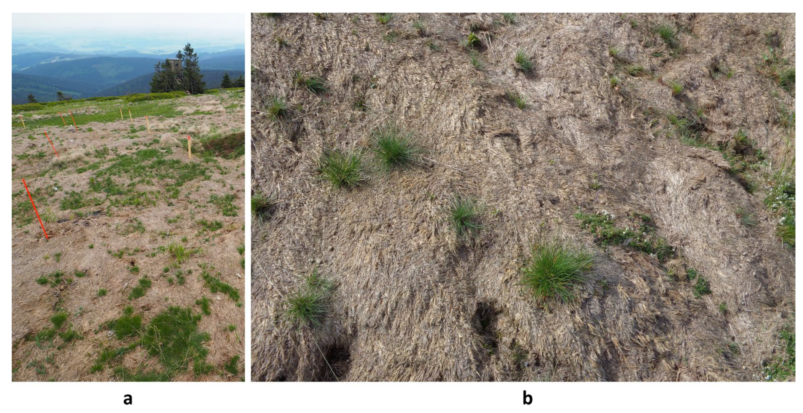
Figure 2.
Study area with location of field points used for the field validation of land cover categories (1 – unvegetated, 2 – dead grassland, 3 – windswept grassland, 4 – dense grassland).
Figure 2.
Study area with location of field points used for the field validation of land cover categories (1 – unvegetated, 2 – dead grassland, 3 – windswept grassland, 4 – dense grassland).
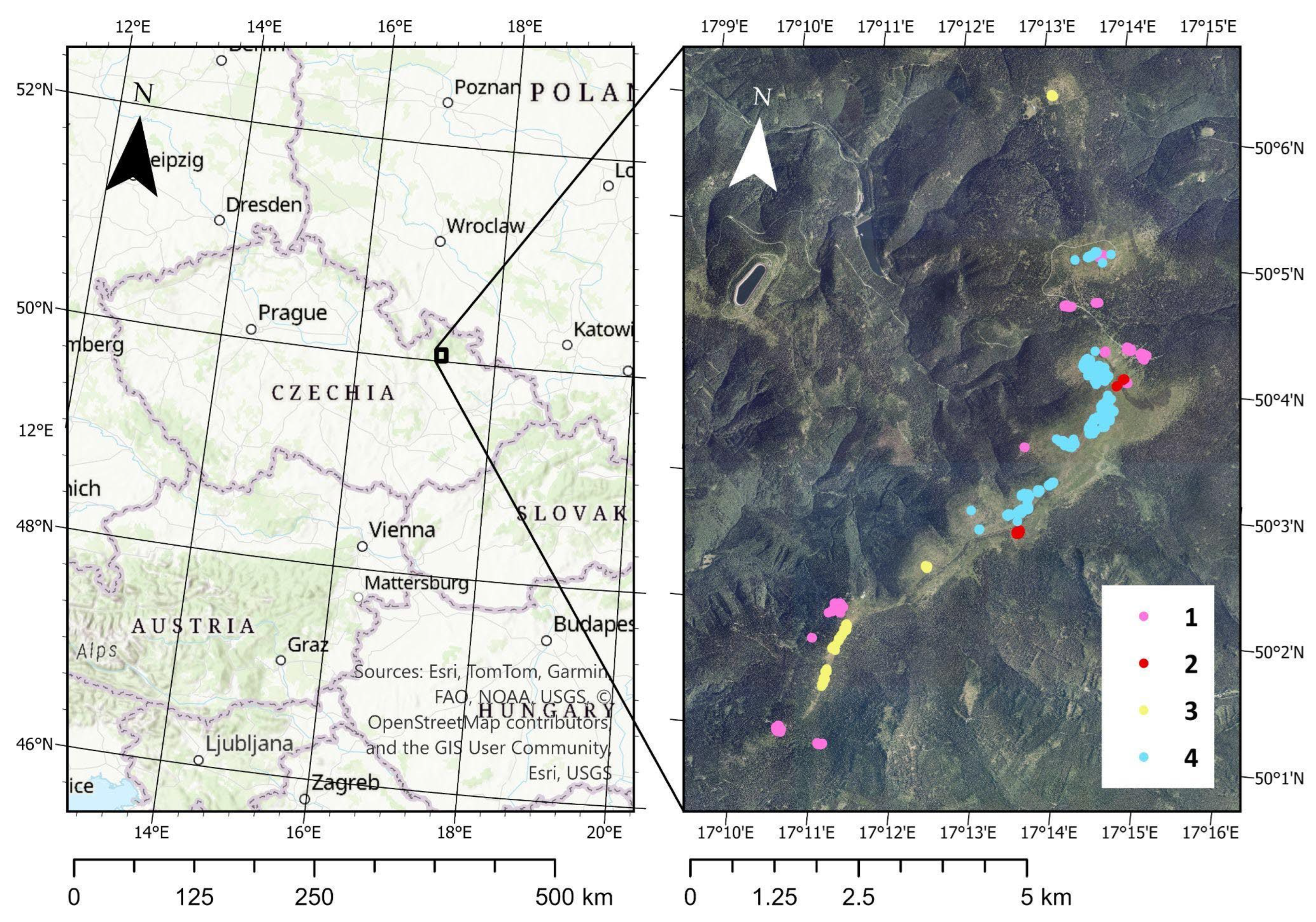
Figure 3.
Boxplots of NPV index values for four land cover classes: (1) unvegetated surfaces, (2) dead grassland, (3) windswept grassland, and (4) dense grassland. Boxes indicate the interquartile range (Q1–Q3), horizontal lines represent medians, and whiskers extend to 1.5× the interquartile range. Numeric labels denote Q1–Q3 values. Statistical significance of pairwise differences among classes was evaluated using Tukey’s HSD test (*** p < 0.001).
Scheme 1.
Workflow for grassland diebacks detection and mapping.
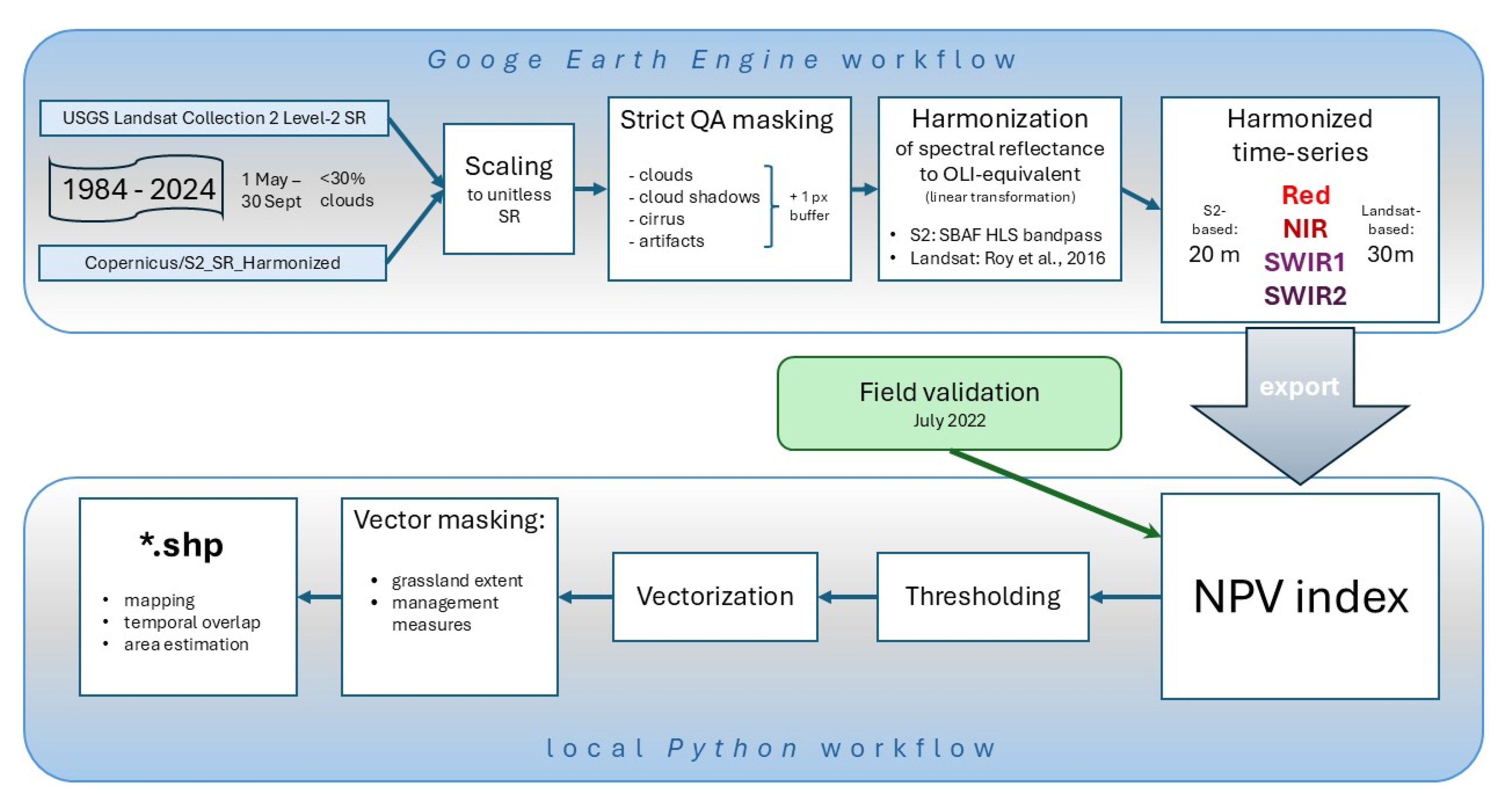
Figure 4.
Spatial extent of four subalpine grassland dieback events: 2000 (a), 2003 (b), 2012 (c), and 2019 (d).
Figure 4.
Spatial extent of four subalpine grassland dieback events: 2000 (a), 2003 (b), 2012 (c), and 2019 (d).
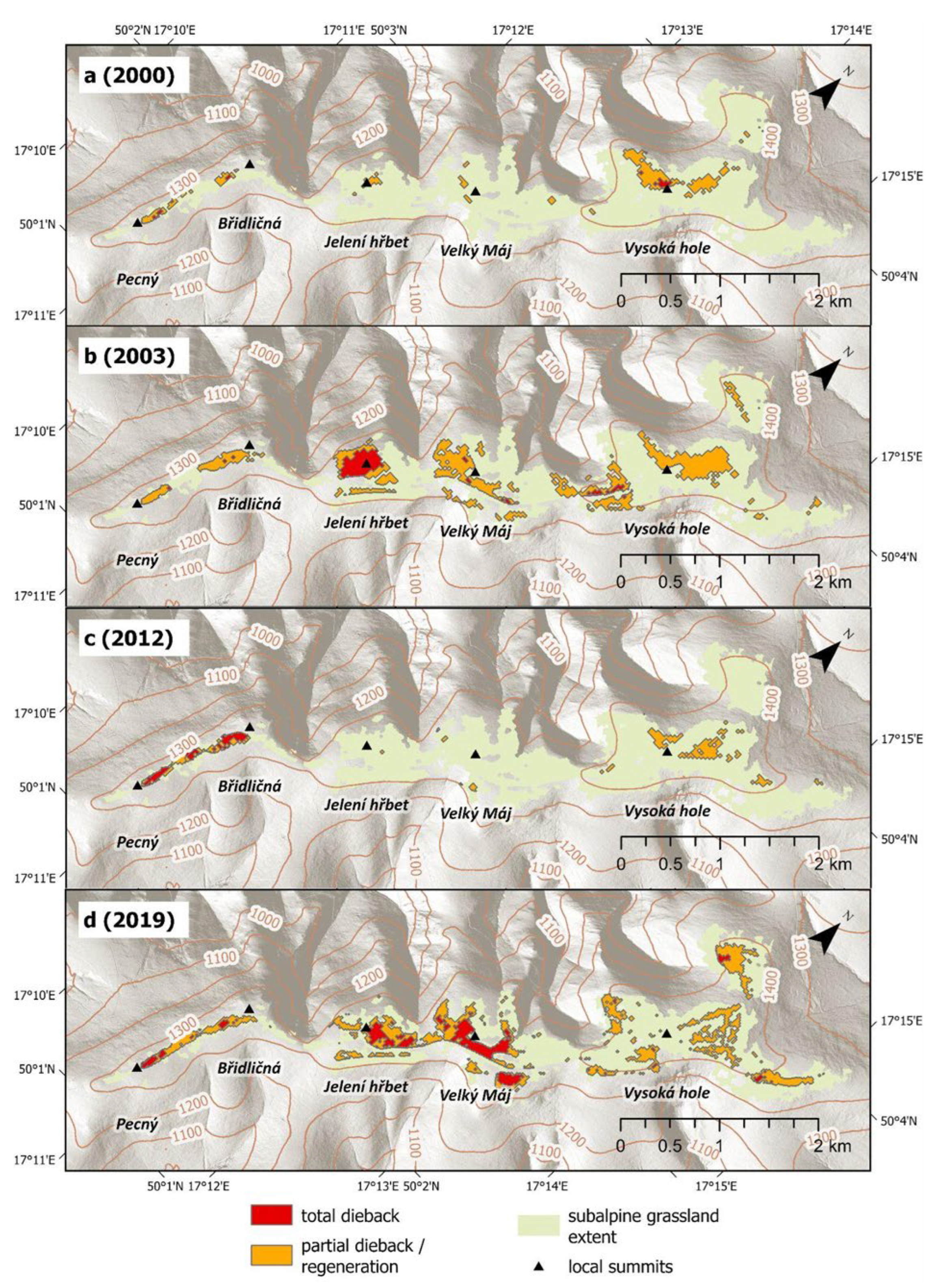
Figure 5.
Duration of dieback persistence at specific locations during the study period (2000–2024).
Figure 5.
Duration of dieback persistence at specific locations during the study period (2000–2024).
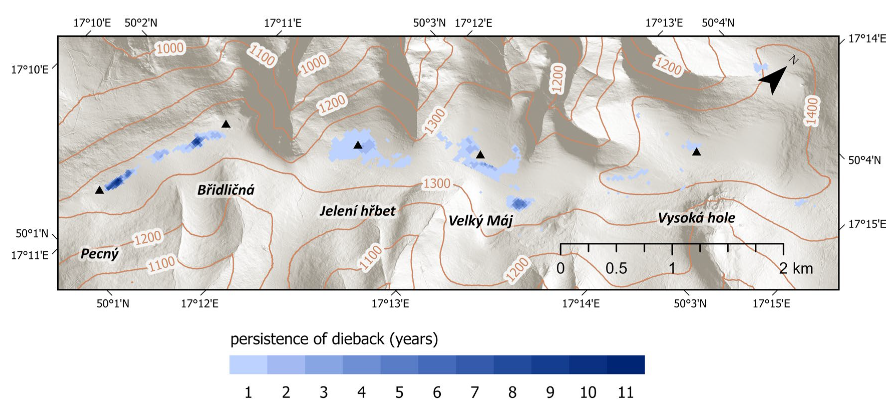
Figure 6.
Subalpine grassland dieback in 2003: (a) RGB orthophoto from August 2003 (source: Mapy.cz © Seznam.cz, a.s. and partners); (b) Normalized Burn Ratio (NBR) derived from Landsat 5 imagery acquired on 11 August 2003, resampled to a 5 m grid for visualization purposes.
Figure 6.
Subalpine grassland dieback in 2003: (a) RGB orthophoto from August 2003 (source: Mapy.cz © Seznam.cz, a.s. and partners); (b) Normalized Burn Ratio (NBR) derived from Landsat 5 imagery acquired on 11 August 2003, resampled to a 5 m grid for visualization purposes.
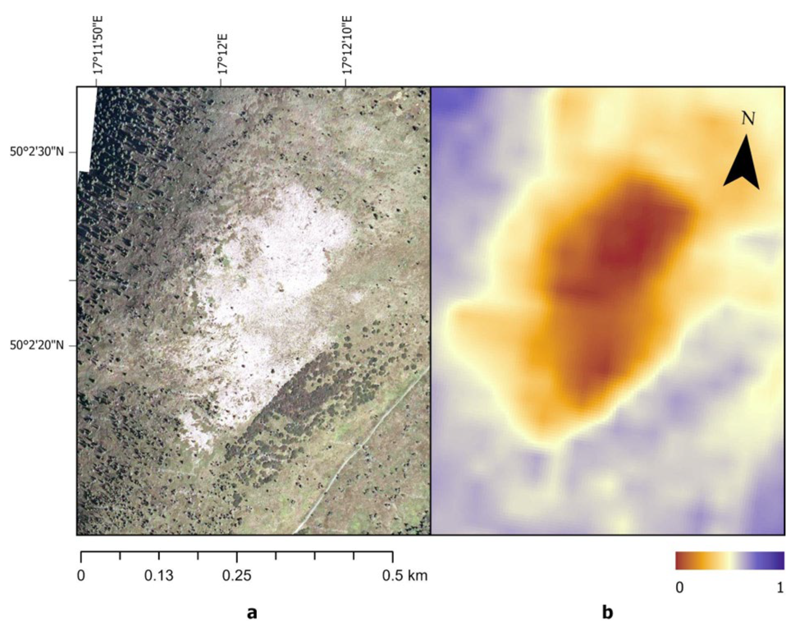
Figure 7.
Subalpine grassland dieback in 2012: (a) RGB orthophoto acquired on 19 August 2012 (source: Czech Office for Surveying, Mapping and Cadastre, ČÚZK); (b) Normalized Burn Ratio (NBR) derived from Landsat 7 imagery (composite of 16 June and 11 September 2012), resampled to a 5 m grid for visualization purposes.
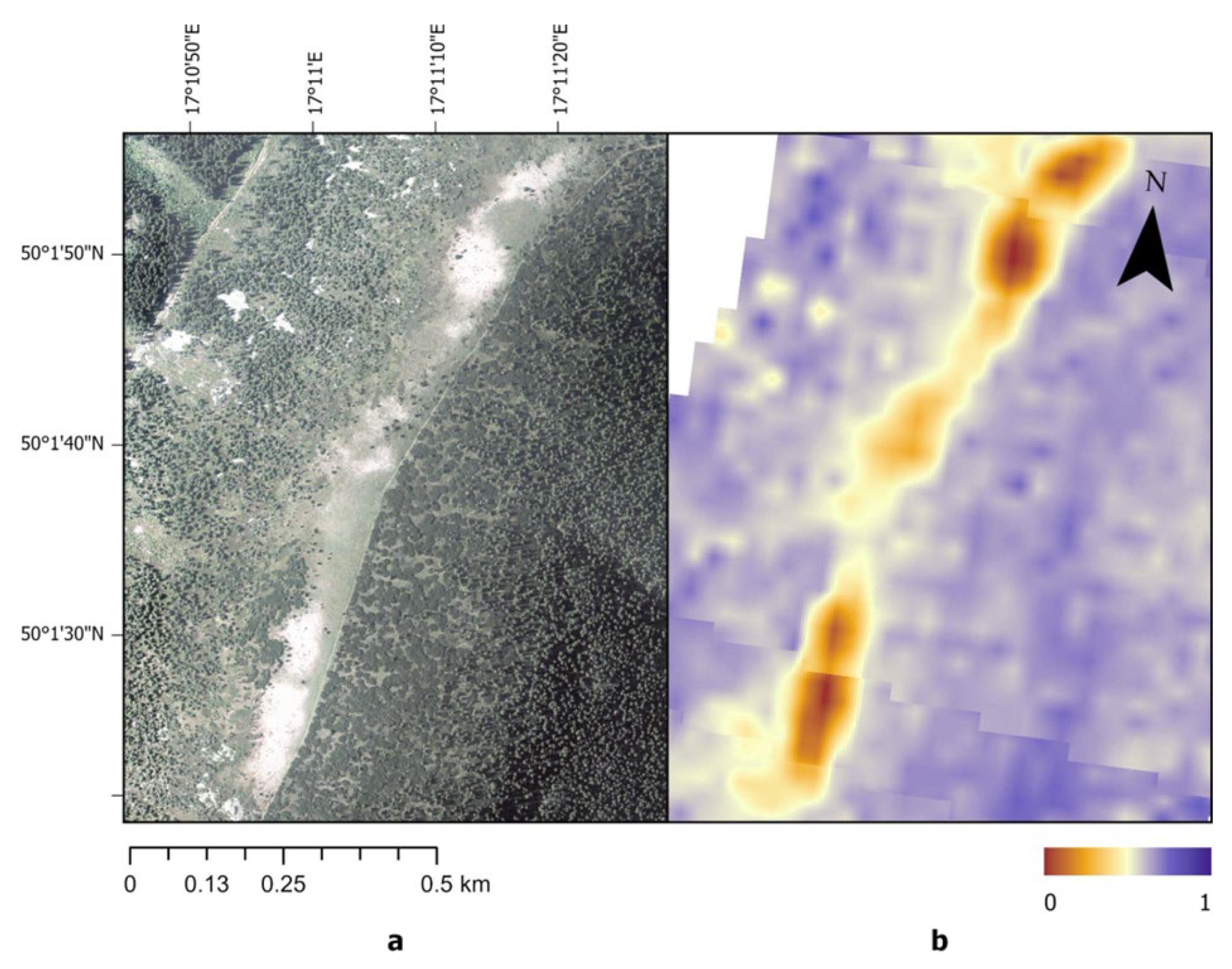
Figure 8.
Seasonal trajectories of mean NBR values for grasslands affected by dieback at four localities (a) to (d). Shaded areas indicate the interquartile range. The black curve represents the reference period (1984–1999), while coloured curves correspond to individual dieback years. Horizontal dashed lines indicate NBR thresholds used to classify dead and damaged vegetation.
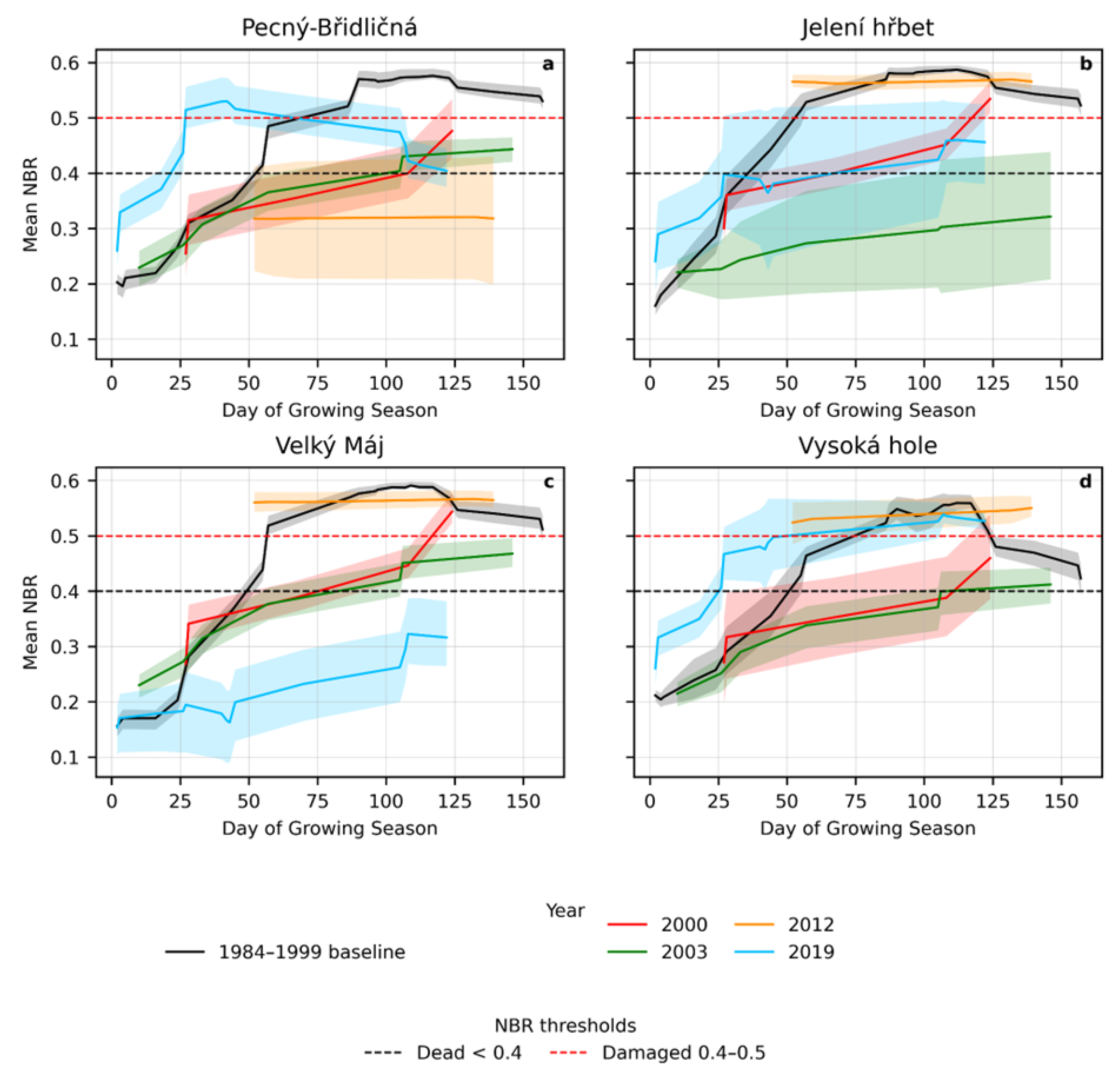
Figure 9.
(a) Relative importance of geomorphological predictors derived from Random Forest classification; (b) Standardized coefficients from binary logistic regression indicating the direction and strength of relationships between predictors and dieback occurrence.
Figure 9.
(a) Relative importance of geomorphological predictors derived from Random Forest classification; (b) Standardized coefficients from binary logistic regression indicating the direction and strength of relationships between predictors and dieback occurrence.
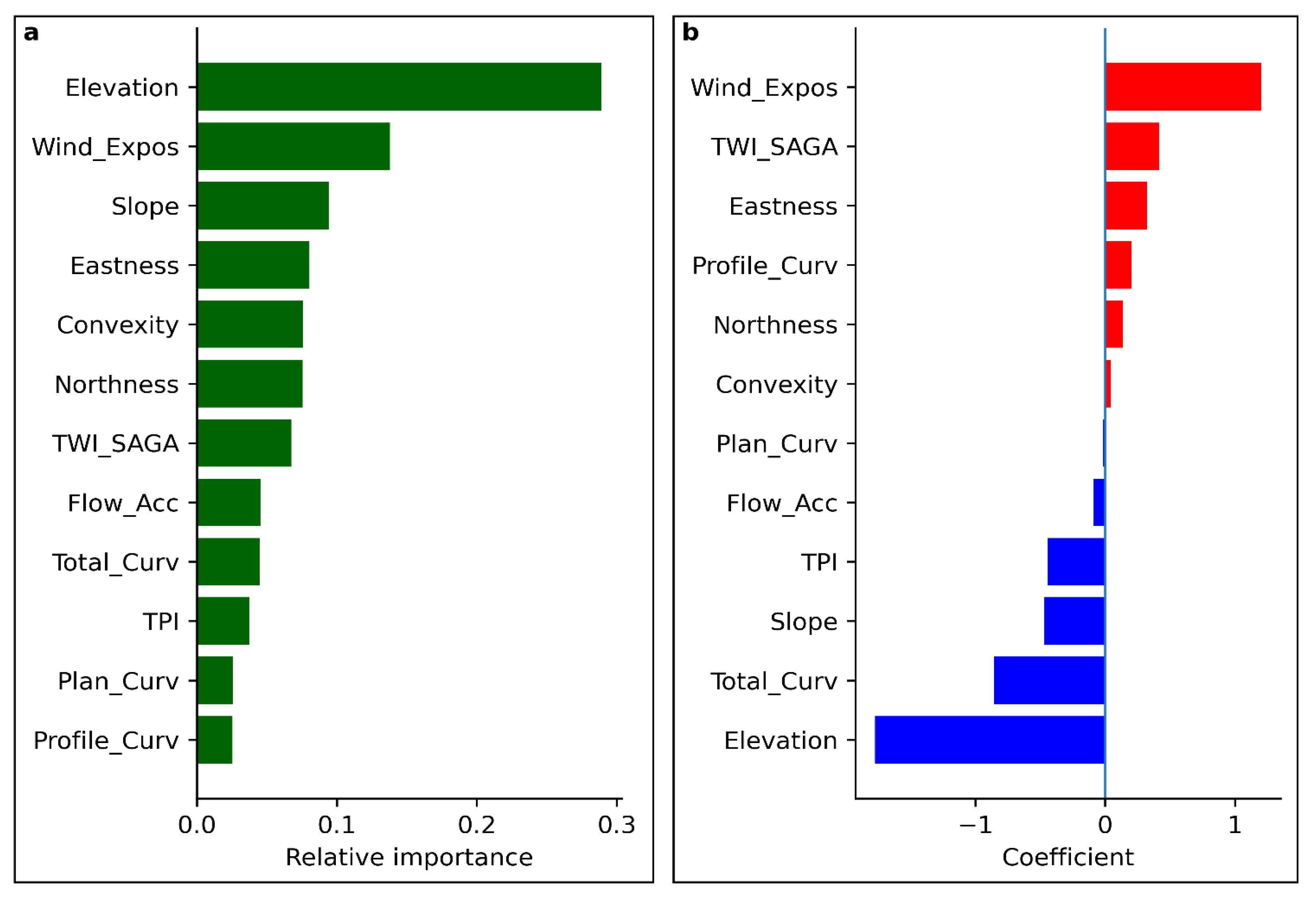
Figure 10.
Standardized Precipitation–Evapotranspiration Index (SPEI-3, SPEI-6, and SPEI-12) in a weekly step (a); and the annual extent of total and partial subalpine grassland dieback/regeneration (b).
Figure 10.
Standardized Precipitation–Evapotranspiration Index (SPEI-3, SPEI-6, and SPEI-12) in a weekly step (a); and the annual extent of total and partial subalpine grassland dieback/regeneration (b).
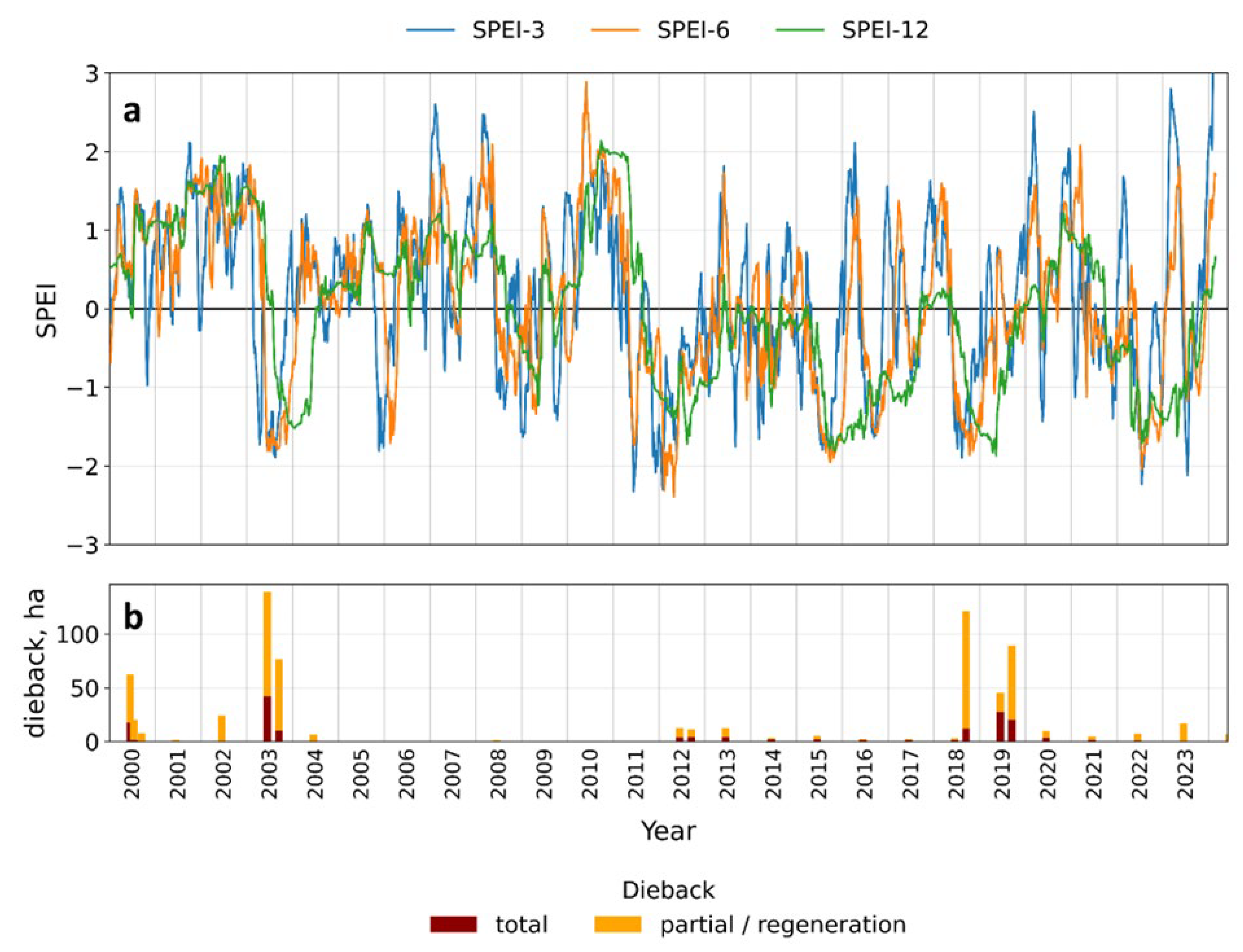

Table 1.
Candidate NPV-related indices for detecting subalpine grassland dieback, compatible with Landsat 5, 7, 8, 9 and Sentinel-2 sensors.
Table 1.
Candidate NPV-related indices for detecting subalpine grassland dieback, compatible with Landsat 5, 7, 8, 9 and Sentinel-2 sensors.
| Abbreviation | Index formulation | Reference |
|---|---|---|
| DFI | DFI=100×(1−(SWIR2/SWIR1))×(Red/NIR) | [70] |
| NDWI | NDWI = (NIR – SWIR1) / (NIR + SWIR1) | [71] |
| NBR | NBR = (NIR − SWIR2) / (NIR + SWIR2) | [72] |
| NDVI | NDVI = (NIR − Red) / (NIR + Red) | [73] |
| NDSVI | NDSVI = (SWIR1 – Red) / (SWIR1 + Red) | [74] |
| MSI(1) | MSI(1) = SWIR1 / NIR | [75] |
| MSI(2) | MSI(2) = SWIR2 / NIR | [75] |
| NDTI | NDTI = (SWIR1 − SWIR2) / (SWIR1 + SWIR2) | [76] |
| STI | STI = SWIR1 / SWIR2 | [76] |
Table 2.
Absolute Cohen’s d effect sizes for pairwise comparisons between land cover classes.
| NPV index | Cohen’s d (absolute values) | ||
|---|---|---|---|
| unvegetated vs dead | dead vs windswept | windswept vs dense | |
| NBR | 1.51981 | 3.79886 | 2.08758 |
| MSI2 | 1.41773 | 3.77823 | 2.07653 |
| NDWI | 0.69399 | 3.43319 | 1.79646 |
| MSI1 | 0.71761 | 3.33757 | 1.80475 |
| NDTI | 2.36804 | 3.26404 | 1.83914 |
| STI | 2.54613 | 3.13174 | 1.79815 |
| NDVI | 2.20674 | 2.93388 | 1.73470 |
| NDSVI | 2.35602 | 1.89167 | 1.32456 |
| DFI | 0.59534 | 1.76564 | 1.33966 |
Table 3.
Estimated area (ha) of total dieback (T) and partial dieback/regeneration (P) of subalpine grasslands by locality, for individual dieback events and post-event years between 2000 and 2024.
Table 3.
Estimated area (ha) of total dieback (T) and partial dieback/regeneration (P) of subalpine grasslands by locality, for individual dieback events and post-event years between 2000 and 2024.
| Dieback event | Year | Locality | Pecný- Břidličná |
Jelení hřbet | Velký Máj | Vysoká hole | In total | |||||
|---|---|---|---|---|---|---|---|---|---|---|---|---|
| Reference date | T | P | T | P | T | P | T | P | T | P | ||
| I (short-term) |
2000a | 22-Jun | 3.72 | 3.70 | 0.45 | 6.57 | 3.97 | 13.81 | 9.43 | 20.56 | 17.57 | 44.64 |
| 2000b | 2-Aug | 0.61 | 3.56 | 0.00 | 1.34 | 0.00 | 1.35 | 0.99 | 12.50 | 1.60 | 18.75 | |
| 2000c | 18-Aug | 0.00 | 0.45 | 0.00 | 0.17 | 0.00 | 0.00 | 0.18 | 6.94 | 0.18 | 7.56 | |
| 2001 | 28-Jul | 0.00 | 0.00 | 0.00 | 0.00 | 0.02 | 1.63 | 0.00 | 0.00 | 0.02 | 1.63 | |
| 2002 | 24-Aug | 0.00 | 3.30 | 0.00 | 1.39 | 0.00 | 4.72 | 0.09 | 14.76 | 0.09 | 24.17 | |
| II (short-term) |
2003a | 23-Jun | 6.17 | 4.58 | 19.34 | 14.53 | 4.43 | 16.46 | 12.25 | 61.38 | 42.19 | 96.95 |
| 2003b | 11-Aug | 0.27 | 7.48 | 8.27 | 8.75 | 0.63 | 20.29 | 1.24 | 29.31 | 10.41 | 65.83 | |
| 2004 | 29-Aug | 0.00 | 0.12 | 0.18 | 2.87 | 0.00 | 0.05 | 0.00 | 3.25 | 0.18 | 6.29 | |
| 2005 | 30-Jul | 0.00 | 0.00 | 0.00 | 0.36 | 0.00 | 0.01 | 0.00 | 0.18 | 0.00 | 0.55 | |
| 2006 | 17-Jul | 0.00 | 0.00 | 0.00 | 0.00 | 0.00 | 0.05 | 0.00 | 0.00 | 0.00 | 0.05 | |
| 2007 | 5-Aug | 0.00 | 0.00 | 0.00 | 0.00 | 0.00 | 0.05 | 0.00 | 0.00 | 0.00 | 0.05 | |
| 2008 | 31-Aug | 0.00 | 0.00 | 0.00 | 0.00 | 0.00 | 0.23 | 0.00 | 1.08 | 0.00 | 1.31 | |
| 2009a | 17-Jul | 0.00 | 0.00 | 0.00 | 0.00 | 0.00 | 0.00 | 0.00 | 0.09 | 0.00 | 0.09 | |
| 2009b | 2-Aug | 0.00 | 0.00 | 0.00 | 0.00 | 0.00 | 0.04 | 0.00 | 0.00 | 0.00 | 0.04 | |
| 2010 | 21-Aug | 0.00 | 0.47 | 0.00 | 0.00 | 0.00 | 0.00 | 0.00 | 0.09 | 0.00 | 0.56 | |
| 2011 | 29-Jun | 0.00 | 0.00 | 0.00 | 0.00 | 0.00 | 0.14 | 0.00 | 0.09 | 0.00 | 0.23 | |
| III (long-term) |
2012a | 23-Jun | 3.88 | 2.42 | 0.00 | 0.00 | 0.00 | 0.04 | 0.00 | 6.38 | 3.88 | 8.84 |
| 2012b | 4-Sep | 3.98 | 1.75 | 0.00 | 0.09 | 0.00 | 0.66 | 0.00 | 4.95 | 3.98 | 7.45 | |
| 2013 | 29-Jul | 2.72 | 3.43 | 0.00 | 0.18 | 1.33 | 4.36 | 0.00 | 0.45 | 4.05 | 8.42 | |
| 2014 | 9-Aug | 1.83 | 1.51 | 0.00 | 0.00 | 0.00 | 0.00 | 0.00 | 0.00 | 1.83 | 1.51 | |
| 2015 | 20-Aug | 1.73 | 3.65 | 0.00 | 0.00 | 0.00 | 0.00 | 0.00 | 0.00 | 1.73 | 3.65 | |
| 2016 | 21-Jul | 1.52 | 1.06 | 0.00 | 0.00 | 0.00 | 0.09 | 0.00 | 0.00 | 1.52 | 1.15 | |
| 2017 | 1-Aug | 1.36 | 1.28 | 0.00 | 0.00 | 0.00 | 0.00 | 0.00 | 0.03 | 1.36 | 1.31 | |
| 2018a | 5-Jul | 1.24 | 1.26 | 0.00 | 0.00 | 0.00 | 0.41 | 0.00 | 0.00 | 1.24 | 1.67 | |
| 2018b | 9-Aug | 8.64 | 3.26 | 0.16 | 20.41 | 2.68 | 32.01 | 0.51 | 53.88 | 11.99 | 109.56 | |
| IV (long-term) |
2019a | 25-Jul | 0.28 | 1.64 | 9.83 | 4.24 | 17.46 | 11.54 | 0.00 | 0.25 | 27.57 | 17.67 |
| 2019b | 31-Aug | 2.14 | 7.22 | 4.82 | 11.21 | 11.61 | 15.54 | 1.74 | 35.18 | 20.31 | 69.15 | |
| 2020 | 31-Jul | 2.08 | 3.20 | 0.00 | 0.20 | 1.43 | 2.88 | 0.00 | 0.01 | 3.51 | 6.29 | |
| 2021 | 15-Aug | 0.28 | 0.68 | 0.00 | 0.12 | 0.90 | 2.86 | 0.00 | 0.13 | 1.18 | 3.79 | |
| 2022 | 5-Aug | 0.16 | 1.27 | 0.00 | 0.50 | 0.80 | 2.70 | 0.00 | 1.82 | 0.96 | 6.29 | |
| 2023 | 25-Aug | 0.00 | 3.76 | 0.00 | 2.55 | 0.54 | 4.50 | 0.00 | 5.55 | 0.54 | 16.36 | |
| 2024 | 12-Aug | 0.00 | 1.31 | 0.00 | 0.73 | 0.16 | 2.06 | 0.00 | 2.57 | 0.16 | 6.67 | |
Disclaimer/Publisher’s Note: The statements, opinions and data contained in all publications are solely those of the individual author(s) and contributor(s) and not of MDPI and/or the editor(s). MDPI and/or the editor(s) disclaim responsibility for any injury to people or property resulting from any ideas, methods, instructions or products referred to in the content. |
© 2026 by the authors. Licensee MDPI, Basel, Switzerland. This article is an open access article distributed under the terms and conditions of the Creative Commons Attribution (CC BY) license.
Copyright: This open access article is published under a Creative Commons CC BY 4.0 license, which permit the free download, distribution, and reuse, provided that the author and preprint are cited in any reuse.


