Submitted:
10 February 2026
Posted:
11 February 2026
You are already at the latest version
Abstract
Background: some widely used wildland fire behavior models like FARSITE propagate fire fronts by computing the front-normal velocity (spread rate) as a function of local inputs and the front-normal direction. Such models are sometimes observed to cause the collapse of crown fires into sharp wedge shapes that eliminate heading fire behavior. Aims: we set out to document this phenomenon, and more generally understand the relationships between fire shapes and spread rate functions. Methods: the phenomenon is studied both mathematically and through simulation experiments. Non-smooth fire fronts are theorized mathematically by an Eikonal partial differential equation ($H(x, \tau, D\tau) = 1$), where the unknown $\tau(x)$ is the time-of-arrival function and the Hamiltonian $H(x, t, p)$ is positively homogeneous and possibly non-convex in $p$; convex analysis is used to study viscosity solutions in constant conditions. Results: we show that a fire spread model preserves the smoothness of fire fronts if and only if it is equivalent to using the Huygens principle. Non-trivially, this is equivalent to a convexity criterion on the inverse spread rate profile, which is then the polar dual of the Huygens wavelet; this corresponds to Hamiltonian-Lagrangian duality. The relevance of smoothness-destroying models to crown fire is debated. Exact analytical formulas are derived for fire growth in spatially constant conditions. Conclusions: our understanding of fire spread models is improved by solving the spread equations in more general ways than previously known. In particular, the collapse of heading crown fires into sharp shapes is now explained. Smoothness-destroying spread models cannot be simulated by algorithms based on travel time like cellular automata; their general well-definedness remains an open question. Fire modelers can use these findings to guide their search for improved crown fire models, and more generally to verify the accuracy of numerical implementations.
Keywords:
wildfire
; fire behavior modelling
; crown fire
; huygens principle
; legendre-fenchel trans-form
; viscosity solution
; Hopf formula
; nonconvex Hamiltonian
1. Introduction
There is considerable interest in accurately modeling the impacts of real or hypothetical wildland fires [1]. One approach consists of using fire spread models in computer simulations that aim to approximately recreate the behavior of real-world fires [2]. Crown fire is a critical aspect of fire behavior modeling, as the onset of crown fire can cause major increases in the intensity and velocity of fire fronts [3]. Some models represent fire spread through highly sophisticated systems of equations [4,5,6], but some very commonly used models like FARSITE [7] simply represent the speed of the fire front as a function of the front-normal unit vector. This paper studies some surprising implications of such models when crown fire occurs. Our main insights come from deriving general analytical formulas that solve the fire spread equations under constant conditions.
In their simplest form, fire spread models propagate fire fronts by using the Huygens principle [8,9]: fire is assumed to grow from an ignition point into a pre-determined wavelet shape (typically, an ellipse), and the fire front is grown by treating the burned perimeter as an infinity of secondary ignition points, and merging the resulting wavelets. Some front-tracking methods, like cellular automata [10] or the Minimal Travel Time algorithm [11], are naturally described and readily implemented in terms of Huygens wavelets. Others numerical methods, such as the Level Set method [12,13] or those based on polygon representations of the fire front, need to convert the wavelet shape into a front-normal spread rate that depends on the direction normal to the fire front (see [14]); we call these speed-from-tangent models, a notion that we define more precisely in Section 2.2. The principle of speed-from-tangent models has been clearly stated by [14]:
The basic premise of the model is that the rate of spread at any point on the perimeter is a function of the angle between the normal vector to the curve and the effective wind direction, with the functional relationship corresponding to that of equilibrium phase fire growth for the fuel and effective wind velocity instantaneously occuring at the point and time in question.
Thus, we are dealing with two classes of models: Huygens wavelet models, and speed-from-tangent models. We saw that some elliptical Huygens wavelet models are equivalent to a speed-from-tangent model, and that some simulation algorithms rely on this equivalence for their implementation. It is natural to ask what the intersection of these two classes is: which Huygens wavelet models are equivalent to a speed-from-tangent model, and vice-versa? This paper fully solves this question, using concepts from convex analysis [15]: every Huygens wavelet model is equivalent to some speed-from-tangent model, but the converse is not true, and the connection between wavelet shapes and spread rate functions is a matter of convex duality. More precisely, the Legendre-Fenchel transform (Section 2.4) is the key tool to convert between the wavelet shape and the (inverse) spread rate function; a speed-from-tangent model is equivalent to a Huygens wavelet model if and only if its inverse spread rate function satisfies a convexity criterion (see Proposition 1 of Section 2.5).
Fire spread models are complicated by the inclusion of crown fire modeling components [3,16]. Models will resolve surface fire behavior using a Huygens wavelet model, then test whether the surface front-normal spread rate is high enough to trigger crown fire initiation [7], in which case the front-normal spread rate might be increased by crown fire. These models are still speed-from-tangent models, but it is no longer clear that they are equivalent to Huygens wavelet models. This paper shows when the equivalence doesn’t hold, with challenging consequences in terms of model well-definedness and numerical accuracy.
In particular, it has been observed that fire simulations sometimes yield sharp pointed fire shapes in conditions conducive to crown fire (see for example color plate 7 of [7], as well as Figure 11 of the present paper). This paper documents this surprising phenomenon more precisely, showing that these conditions yield to the collapse of heading crown fire into pointed shapes: said informally, heading fire orientations of the fire front are not sustainable, because heading fire advances so fast compared to other orientations that it “rips itself free” from the fire perimeter. We study the phenomenon both theoretically and experimentally, showing that these conditions correspond to violating the above-mentioned convexity criterion of the inverse spread rate function, and that some numerical algorithms will yield inconsistent and incorrect predictions in these conditions. Importantly, we show empirically that the phenomenon can still happen in non-constant conditions, although its prevalence in practice remains an open question.
This collapse into a sharp shape is not a numerical artifact, but a mathematical inevitability. This raises questions about the well-definedness of the model: indeed, speed-from-tangent models rely in their definition on resolving the tangent to the fire front, and yet they yield sharp fire fronts where the tangent does not always exist. Other scientific fields have grappled with this problem before, and solved it through the notion of weak solutions to partial differential equations [17]. There are several approaches to defining weak solutions, but what seems to have emerged is the notion of viscosity solution [18,19]. This paper adopts this approach: in Section 2.7, we reframe fire spread with speed-from-tangent models as equivalent to solving a certain partial differential equation (namely, an Eikonal equation with a positively homogeneous Hamiltonian, possibly discontinuous and non-convex, see Equation 20 of Section 2.7.2), and study the corresponding viscosity solutions. The convexity criterion we mentioned above corresponds exactly to the convexity of the Hamiltonian.
To the authors’ knowledge, our Equation 20 is the first occurrence in the wildfire literature of front-propagation models like FARSITE [7] and ELMFIRE [13] being formalized mathematically in a way that allows for sharp fire fronts while accounting for the loss of regularity caused by their approach to crown fire modeling. We note that previous works have studied very similar problems in more sophisticated systems of equations for fire spread such as reaction-diffusion systems [4,5,6] which include small-scale effects. [4] and [5] are especially similar to the present paper, thus supporting our approach of studying viscosity solutions; however, the Hamiltonians considered in these works are always convex, and therefore cannot cover the full range of situations studied in this paper. More generally, we have found it difficult to find previous works in the Hamilton-Jacobi literature that cover the convexity and continuity violations that we have to deal with for crown fire modeling, presumably because the Hamiltonian is naturally convex in most problem spaces and because discontinuity is a very nasty assumption to deal with. Also note that [20] and [21] might seem superficially similar to the present analysis, but they studied a much narrower problem of isotropic fire spread.
For model design and verification purposes, it is useful to compare simulated fire perimeters to correct fire perimeters derived from theory, in situations that are simple enough to be solved analytically. Historically, this has been done by simulating fires from point ignitions in constant conditions that yield either only surface fire or only crown fire, because then the fire perimeter would be an ellipse of known shape (see for example [22]). The mathematical theory derived in this paper solves this problem in much more general settings: in particular, we provide formulas (Equations 16, 24 and 41) for any convex initial burned region in any set of spatially constant conditions, even in the challenging cases that yield a mix of surface and crown fire violating the convexity criterion.
The above tells us what correctly implemented simulation algorithms should predict, but not whether that the underlying model is desirable. There are reasons to be distrustful of sharp fire fronts and heading fire collapse: does it make sense that heading crown fire is unsustainable? Does it make sense that the heading fire gets narrower as the fire spreads? Some modelers might brush the issue aside by simply deciding that sharp fire fronts are unphysical, thus following the assumptions of [14]. We are more nuanced, because some evidence suggests that pointed shapes might be a natural phenomenon [23]: this is discussed in Section 4.
These findings are arguably of high relevance to authors of wildland fire spread models, by raising their awareness of sharpness in predicted fire fronts, and helping them address it:
- If they want to disallow sharpness in predicted fire fronts and preserve the Huygens principle, the convex duality of Section 2.4 will guide their search for suitable spread rate functions or wavelet shapes.
- If they do want to allow sharpness, Section 2.7 and Section 2.8 will help them verify the accuracy of their numerical algorithms.
This paper is structured as follows. Section 2.1 briefly recalls some mathematical foundations. Section 2.2 defines what we call speed-from-tangent models (the class of models studied in this paper) and what it means for them to be smooth-growing, i.e. to preserve the smoothness of the fire perimeter over time. Section 2.3 defines and studies fire spread using the Huygens principle [9], showing that such models are a subclass of speed-from-tangent models that are smooth-growing. Section 2.4 then introduces the polar Legendre-Fenchel transform, which will be instrumental to studying the convex duality between fire (wavelet) shape and spread rate profiles. This is leveraged by Section 2.5 to show that smooth-growing models are exactly those following the Huygens principle, such that the wavelet shape and inverse spread rate profile are conjugate via the polar Legendre-Fenchel transform (proposition 1). Section 2.6 further characterize such models as convolutions, and derive a first round of analytical formulas for constant-conditions spread. Section 2.7 then moves on to theorize models that are not smooth-growing, by studying viscosity solutions of the Eikonal equation: in particular, Proposition 2 provides an analytical formula for the evolution of the fire front from a convex initial burned region in constant conditions, which notably explains the collapse of smooth perimeters into sharp pointed shapes. Section 2.8 generalizes these results to time-varying conditions. Finally, Section 2.9 describes simulation experiments we conducted to confirm and complement the theoretical results, the results of which are analyzed in Section 3. Section 4 discusses the implications of these findings, relates them to other scientific fields, and lays out potential directions for future research. Finally, Section 5 summarizes the above.
Readers in a hurry might want to go straight to Figure 6, which captures much of the insights from this paper in one self-contained visual explanation.
2. Materials and Methods
This section mostly studies the mathematical properties of speed-from-tangent models (defined in Section 2.2), with Huygens wavelet models (defined in Section 2.3) as a special case. In addition, Section 2.9 describes the design of the simulation experiments conducted in this study. For reference, Table 1 summarizes the notation used in this paper, which will be introduced as needed.
2.1. Mathematical Definitions
In this paper, the symbol represents an azimuth, i.e. an angle indicating a direction. Functions denoted are always assumed to be -periodic, i.e. ; this simply says that the value of is fully determined by the direction represented by .
A subset S of the plane is said to be convex if S contains the line segment joining any two of its points [15,24]. The intersection of two or more convex sets is convex.
We define the radial graph of a function as the set of points of the plane described by the polar-coordinates equation . Intuitively, f can be viewed as a closed curve in the plane, and the radial graph is the set of points inside that curve.
We will say that a function is polar-convex if its radial graph is convex. See Figure 1 for an illustration. The visual intuition is that the curve of f delineates a convex shape. A polar-convex function is always continuous, but not necessarily smooth: it may have sharp “corners”. Not all continuous functions are polar-convex. Polar-convexity is the most important regularity condition in this paper.
2.2. Speed-from-tangent Models
The most general class of fire spread models studied in this paper is what we call speed-from-tangent models. The fire spread components of models like FARSITE, Prometheus, ELMFIRE and Pyretechnics [7,13,25,26] are instances of speed-from-tangent models.
Speed-From-Tangent Models are defined as follows. In a given set of environmental conditions (wind, fuels, topography, etc.), the front-normal spread rate (in m/s) is fully determined by the unit vector normal to the fire front (or equivalently, by the direction tangent to the front, hence the name “speed-from-tangent”). What we call the front-normal spread rate is the velocity at which the fire front advances in the direction perpendicular to itself. See Figure 2 for a schematic illustration. This means that the model can be described by a spread rate function , in which is an azimuth (in radians) representing the front-normal direction, C captures environmental conditions like fuels and wind, and is a speed in m/s. To keep notation lightweight, we will make the dependency on C implicit and just write . Typically, will be highest in the downwind or upslope direction.
The function is typically specified as follows, based on physical and empirical modeling arguments that involve both surface and crown fire:
- 1.
- A surface fire spread rate is derived from an elliptical wavelet model (see Section 2.3) [8,9]. The dimensions of the wavelet are determined using Rothermel’s model [27,28], along with a model that determines a length/width ratio. A fireline intensity (in kW/m) is derived from using Byram’s equation [29].
- 2.
- If exceeds a threshold, crown fire occurs. Then, another elliptical wavelet model is applied for crown fire, yielding a spread rate .
- 3.
- and are combined in some way to yield the actual spread rate , for example by taking the maximum of the two: . Some models like FARSITE use more sophisticated logic, but the results of this paper will still be applicable to them.
2.2.1. Smooth-Growing Models
Not all possible functions are necessarily valid or reasonable; this paper is interested in finding constraints on that ensure well-behaved fire growth in simulations. In particular, note that speed-from-tangent models have historically [14] been based on the assumption that the front-normal direction can always be resolved, whereas the onset of pointed fire shapes contradicts this assumption. This compels us to define the following regularity condition: we will say that is smooth-growing if it essentially preserves the smoothness of fire perimeters over time. More precisely, we adopt the following definition:
Definition 1
(Smooth-growing models). A speed-from-tangent model issmooth-growingif a fire front which is R-propagated from a circular initial front at time has a tangent at all points for all .
Note: it might seem arbitrary to require the initial perimeter to be circular. It will become clear in later sections that this arbitrariness is inconsequential: what matters is that the initial burned region be smooth, bounded, and convex. Convexity is an important assumption because smoothness might be destroyed by the merging of fire fronts even if R is highly regular.
Section 2.5 will provide necessary and sufficient conditions for a function to be smooth-growing.
2.3. Huygens Wavelet Models
Another approach to modeling fire spread is to use a Huygens wavelet model [8,9]. A Huygens wavelet specifies the shape of a fire growing around a point of ignition as a function (in m/s): in direction , the fire grows a distance from the point of ignition for a duration . In other words, the burned region when spreading a fire from the origin for a duration is the radial graph of .
A Huygens wavelet model spreads fires as follows: the burned region at time is obtained by merging all the duration- wavelets from the burned region at time t, as if the time-t burned region consisted of an infinity of secondary ignition points (See Figure 3).
Importantly, we must assume that the wavelet function is polar-convex. Polar-convexity is an essential consistency criterion: it ensures that growing a point ignition for duration then yields the same result as growing it for time . It can be seen that polar-convexity is equivalent to satisfying a triangle inequality, i.e. that spreading from point A to point C takes no longer than spreading from A to B then from B to C. The Huygens principle makes essentially no sense without this assumption.
The shape of the wavelet generally varies based on environmental conditions: typically, in fire simulations, drier fuels will yield larger wavelets, and high winds will yield more elongated wavelets. In homogeneous conditions, all points and all instants in time will have the same wavelet function . Then, the function fully describes the growth of the fire perimeter from a point ignition: if a fire is ignited from the origin and grown for duration , the burned region is described in polar coordinates by the equation . In other words, the arrival time of the fire at a point with polar coordinates is equal to .
It can be seen that a Huygens wavelet model implies a speed-from-tangent model , given by the equation:
Surface fire spread algorithms often work by defining a wavelet function , then finding an analytical expression for the right-hand side of equation 1. One way to understand equation 1 is to see that quantifies how fast the -radius of the wavelet is progressing in direction . See Figure 4 for a visual proof. If follows that is the “distance” between the origin and a supporting line of the wavelet which is oriented with normal direction .
Because the wavelet is convex, it is the intersection of the half-planes defined by these supporting lines; it follows that can be recovered from by the equation:
To make sense of equation 2, note that the supporting half-plane with normal direction can be described by the inequality in polar coordinates ; equation 2 follows by substituting and expressing the intersection as an infimum. See Figure 5 for a visual proof. We shall find it interesting to rewrite equation 2 as follows:
Note that W is differentiable (i.e. has a tangent) at if and only if the supremum in equation 3 is strict, i.e. attained at only one point . From this property, along the results that will be derived in Section 2.6, it can be seen that Huygens wavelet models are smooth-growing:
Lemma 1.
Let a Huygens wavelet model.
Then the speed-from-tangent model implied by W is smooth-growing (as defined in Section 2.2.1).
2.3.1. Elliptical Wavelets
To make the above notions more tangible, this section will provide concrete formulas for and in the special case of elliptical wavelets, which are common building blocks in wildfire spread models. The rest of the paper is independent of this section. Let us say that an elliptical wavelet is focalized if it grows around a focus of the ellipse, which is a common modeling choice; then the wavelet function is:
in which is the direction of fastest spread (typically, the downwind direction), is the spread rate in that direction, and e is the eccentricity of the ellipse, which can be expressed in terms of the length-to-width ratio as:
It can then be seen that the front-normal spread rate can be expressed as:
in which is the backing spread rate, and is the flanking spread rate which can be expressed as:
This formula holds even if the elliptical wavelet is not focalized, as long as the point of ignition lies on the main axis of the ellipse.
If W is a focalized wavelet, it can be seen (nontrivially) that describes a circle of diameter . This explains the aspect of some curves that will appear later in this paper. Of course, this circle is generally not centered at the origin.
Note that in typical spread models, the above formulas hold in the plane tangential to the slope. This means that these formulas no longer hold once the wavelets and spread rates are vertically projected onto a horizontal plane, and accounting for slope makes the calculations more complicated (see for example [25]).
2.4. Convex Conjugacy: The Polar Legendre-Fenchel Transform
Definition 2
(Polar Legendre-Fenchel Transform). If is a positive function, then we define itspolar Legendre-Fenchel transform as:
This transform will be important to us, because it reveals the duality between Huygens wavelet and speed-from-tangent models. Indeed, note that equations 1 and 3 from Section 2.3 can be rewritten as:
in which denotes the multiplicative inverse of R, i.e. .
The polar Legendre-Fenchel transform we introduced above plays a similar role to the ordinary Legendre-Fenchel transform [30], but for functions defined by polar coordinates instead of Cartesian coordinates . In particular, it enjoys similar properties:
- 1.
- is polar-convex (even if f is not polar-convex).
- 2.
- (i.e. induces an involution on its image).
- 3.
- .
- 4.
- f is polar-convex if and only if .
- 5.
- is the polar-convex extrapolation of f, i.e. the smallest polar-convex function no smaller than f. Intuitively, one can picture a loop of string being tightened into a convex shape around the curve of f.
- 6.
- If f is polar-convex and , then .
- 7.
- if and only if f is polar-convex at θ, i.e. if the radius of f in direction touches a supporting line. This essentially means that there is no “concavity” at .
- 8.
- If , then .
- 9.
- .
- 10.
- for any positive scalar .
- 11.
- transforms sharp corners into straight line segments, and conversely.
- 12.
- Let f polar-convex; then is differentiable at is and only if the supremum in equation 8 is attained at exactly one .
As we saw in equations 9 and 10, in the context of Huygens wavelets models, W and are conjugate through the polar Legendre-Fenchel transform. Thus, can help us understand how properties of spread rates translate to properties of wavelets, and vice-versa. For example, because , we have just learned an important property of the spread rate function implied by a Huygens wavelet model: must be polar-convex. As will be shown in Section 2.5, this turns out to be the key requirement for a speed-from-tangent model to be smooth-growing.
The transform we defined here is not conventional: mathematicians tend to use more general definitions. We find our present definition useful to make our analysis self-contained and tailor-suited to two-dimensional front propagation. However, the connections to more general definitions are insightful, and some of them will be explained in Section 2.7.4. In the meantime, we note the following connection to convex geometry: if denotes the radial graph of f and the radial graph of , then , in which denotes the real polar of set A, defined as [15].
2.5. Regularity Property: Smooth-Growing Models are Huygens Wavelets
Recall that we want to characterize which speed-from-tangent models are smooth-growing (Section 2.2.1). We learned from Section 2.3 that how to obtain some smooth-growing models: start from a Huygens wavelet model , then derive R as . It turns out that this is the only way to obtain a smooth-growing model - all smooth-growing models are equivalent to some Huygens wavelet model, as stated in the following proposition:
Proposition 1.
Let be the spread rate function of a speed-from-tangent model. The following propositions are equivalent:
- 1.
- R is smooth-growing.
- 2.
- is polar-convex.
- 3.
- R is the spread rate function implied by some Huygens wavelet model .
When the above applies, then and W are conjugate by the polar Legendre-Fenchel transform: and .
Proof
(Disclaimer: the standard of proof we use here is that of physics, not mathematics. We will not go into checking all mathematical details. Instead, we will give readers an intuitive understanding of the processes at play. Note that this proposition can be more rigorously proved as a corollary of Proposition 2.)
We already know from Lemma 1 (Section 2.3) that a Huygens wavelet model implies a smooth-growing speed-from-tangent model. Therefore, we only prove the reverse implication.
Consider a smooth-growing speed-from-tangent model with spread rate function . It is enough to show that = for some polar-convex function , as this means that our model is equivalent to a Huygens wavelet model. Said informally, the main idea of the proof are that (1) we know how to find the function W: it is the asymptotic shape of the fire perimeter, and (2) is the speed at which the -oriented tangent of the fire perimeter is being pushed away from the origin.
We assume that a fire is grown from a circular initial perimeter, which shape is described by a constant polar-convex function . In a way reminiscent of equation 1, we define a time-varying function which describes how far the fire has advanced in direction at time t. For example, if quantifies radians clockwise from North, and we choose , then is the Northernmost latitude reached by the fire at time t. Denoting the polar-convex function describing the convex hull of the time-t burned region, we have:
... which can be rewritten as .
Because the perimeter is smooth, for any , the supremum in the above equation is attained at some point along the perimeter where the front-normal direction is . Because the front-normal rate of spread is , it follows that
and therefore .
We now choose t to be high enough that the initial perimeter has negligible size compared to the perimeter at time t, so that the approximation holds. Denoting , we thus have . Because is polar-convex, so is W; this completes the proof. □
Some remarks on Proposition 1:
- 1.
- A sufficient condition for being smooth-growing is that R be twice differentiable and .
- 2.
- However, non-smoothness of R is also allowed: sharp angle in the curve of will turn into straight line segments in the curve of .
2.6. Constant-Conditions Wavelet Spread as a Convolution
This section will provide exact expressions for fire growth in constant conditions using Huygens wavelet models. We already know from Section 2.3 how such models grow fires from a point ignition: a fire perimeter grown from the origin can be exactly expressed as , in which is the Huygens wavelet function. The rest of this section will extend this result to arbitrary initial perimeters, by introducing a convolution operation.
Let and two functions; let and be their radial graphs (see Section 2.1), viewed as sets of 2-dimensional vectors. We can consider the set ; it is easily verified that this set is the radial graph of some function (in fact, ). We call g the convolution of and , and denote it by .
It can be seen that the convolution operation is commutative and associative, and that the convolution of polar-convex functions is itself polar-convex. Because set union corresponds to a max operation, the convolution also has a distributivity property: . Furthermore, by reasoning about the position of supporting lines, it can be seen that the polar Legendre-Fenchel transform maps convolutions to sums of inverses:
Homogeneous fire spread with a Huygens wavelet can be viewed as a convolution. Indeed, observe that applying the Huygens principle is equivalent to taking a sum of sets: if is the time-t burned region (viewed as a set of 2-dimensional vectors), then , in which denotes the radial graph of the -scaled Huygens wavelet . It follows that if the initial burned region is the radial graph of some function , and the fire is grown with wavelet for a duration t, then the burned region at time t is the radial graph of some function , which can be expressed as the following convolution:
If we further assume that the initial burned region is convex, we can derive from Equation 14 a more computationally efficient formula to calculate . Indeed, if is polar-convex, then is polar-convex too, therefore . Denoting the spread rate function, and recalling that (Section 2.4), we can then express as:
Equation 15 is interesting both theoretically and computationally. It can be used in validation experiments, to check that a simulated fire perimeter agrees with the one predicted by theory. Equation 15 also reveals that the asymptotic fire shape is insensitive to the initial perimeter, and given by the Huygens wavelet: indeed, as , we have , therefore .
Equation 15 corresponds to the Hopf formula [31] in the Hamilton-Jacobi literature. We will see in Proposition 2 of Section 2.7 that the equation 15 can still be applied to models that do not follow the Huygens principle.
2.7. Viscosity Solutions: Allowing for Sharpness
The previous sections have studied the conditions in which fire spread yields smooth fronts. We now study the possibility of sharpness in the fire front, from models that violate the convexity condition of Proposition 1. This gives us a problem of model definition: a speed-from-tangent model is defined by associating a rate of spread to each front-normal direction ; yet we now need to defined how the model is supposed to behave at sharp corners where the front-normal direction is undefined. Other scientific fields have struggled with this problem, and addressed it through the notion of weak solutions to partial differential equations [17]. We shall take a similar approach:
- 1.
- We will describe fire spread in terms of Time-of-Arrival (ToA) functions , which describe the time at which a spatial point is burned by the fire.
- 2.
- The ToA function must be a solution to a partial differential equation, the Eikonal equation (Equation 20).
- 3.
- Because of sharpness in the fire fronts, the ToA function might be non-differentiable. Therefore, we need to choose some notion of weak solution in order to model the problem. We argue that the notion of viscosity solution [17,19] is suitable and appealing, because of its properties in terms of existence, uniqueness and stability of solutions, and because it is widely adopted for theorizing the propagation of fronts [32].
- 4.
- We will not prove the uniqueness of solutions mathematically, but argue that it is a reasonable assumption to make in Section 2.7.3. Therefore, when we prove that some function is a viscosity solution, we will take for granted that it is the correct solution.
- 5.
- We will prove in Section 2.7.4 that the “polar Hopf Formula” (Equation 15) we introduced in Section 2.6 corresponds to a (the) viscosity solution, even when the assumptions of Section 2.6 (Huygens principle) do not apply. This will give us the exact fire growth in constant conditions, which will be useful both to explain the onset of sharp corners in fire fronts, and to verify the accuracy of numerical algorithms.
Based on the above, we state our generalization of the polar Hopf Formula (Equation 15):
Proposition 2
(Constant-conditions fire growth from a convex initial burned region). We assume a speed-from-tangent model with spread rate function , which is:
- 1.
- bounded above and below: for some velocity constants ;
- 2.
- lower semi-continuous, i.e. if θ is a point of discontinuity.
We consider fire spread in constant conditions using this model, from a bounded convex initial burned region represented by a polar-convex function .
Then the correct time-t fire front (in the sense of viscosity solutions to the Eikonal equation) is described in polar coordinates by , where is the following function:
Proof.
See Section 2.7.4 for existence, and Section 2.7.3 for uniqueness.
Note: the assumption of lower semi-continuity is a technical point that will be justified in Section 2.7.5. □
Let us give a visual interpretation of Proposition 2. The initial burned region being convex, it is the intersection of the half-planes containing it; and we saw in Section 2.3 and Section 2.4 that the transform gives us the location of these half-planes. The boundary of each half-plane can be viewed as an infinite linear fire front that has just burned past the initial burned region. One can imagine letting these linear fire fronts move away from the initial perimeter for a duration t, each at the velocity prescribed by the model, then taking their intersection again. Proposition 2 tells us that this is the correct way of calculating the time-t burned region. This is illustrated in Figure 6.
This also sheds light on the onset of sharp pointed shapes: if lies in a concavity of , the corresponding linear fire front moves so fast that it “escapes” and cannot be tangential to the time-t perimeter (see Figure 6).
Figure 6.
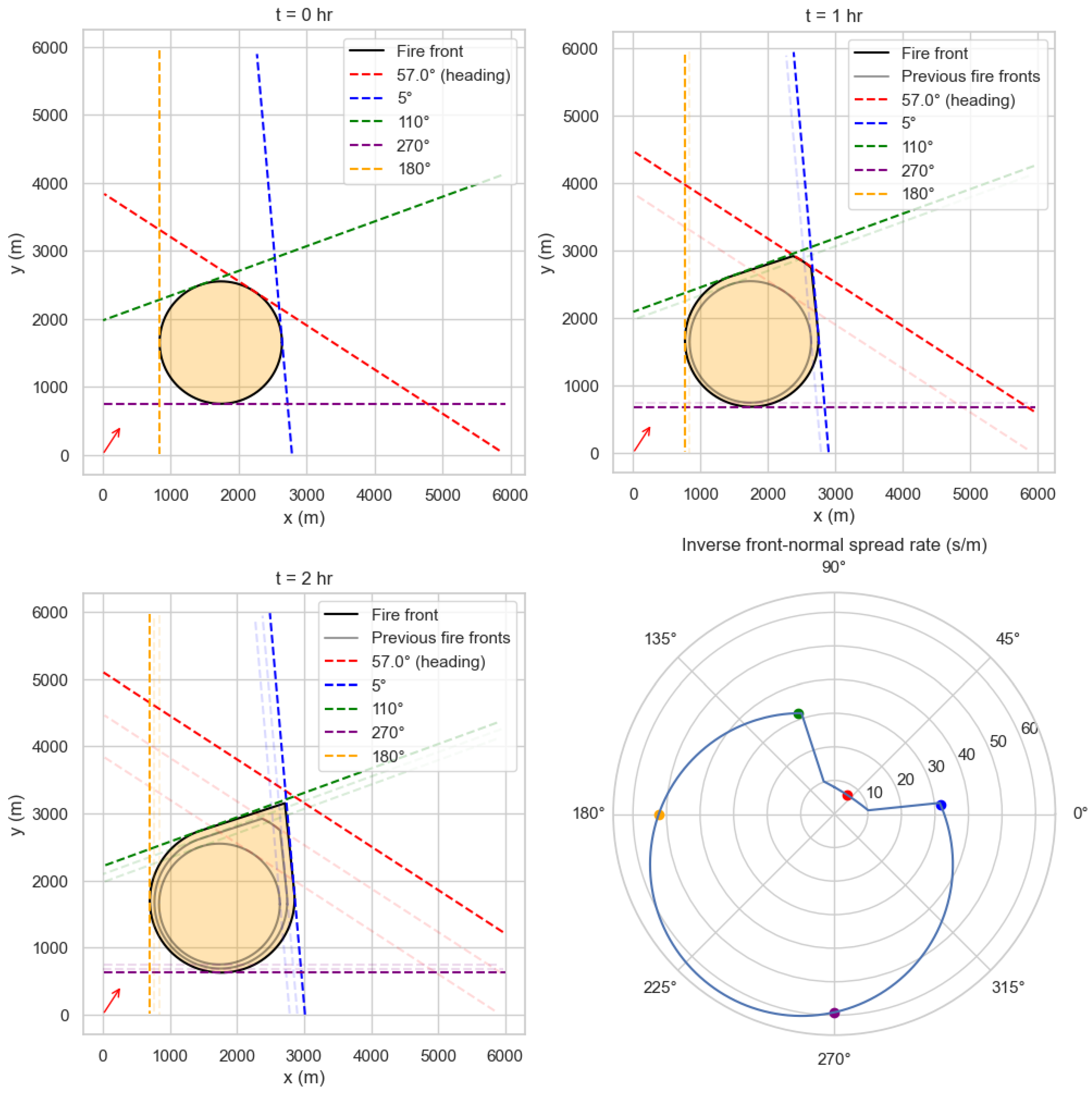
A geometric explanation of fire growth under constant conditions from a convex initial burned region, and how it can lead to the collapse of a heading crown fire into a pointed shape. Black solid curves represent the fire front at various times, with the burned region filled in semitransparent orange. A red arrow indicates the heading fire azimuth - that is, the front-normal direction of fastest spread, which in this example is the downwind direction (57°). The initial fire front (upper left) is decomposed as the envelope delimited by its supporting lines, a few of which are displayed as dashed lines. Each of these lines can be viewed as an infinite linear fire front, and marched forward at the velocity predicted by the model (bottom-right polar plot), yielding new envelopes at later times (top-right and bottom-left plots). The previous positions of the lines are displayed in semitransparent colors. The polar Hopf formula derived in this paper states that this geometric envelope construction correctly calculates the front evolution that follows from the fire spread model. The bottom-right polar plot displays the inverse spread rate function as a light blue curve; colored dots correspond to the lines in other plots. We see sharp changes in spread rates at about 5° and 110°, corresponding to the transition to crown fire. This creates a concavity that shelters the direction of fastest spread (57°, in red): nontrivially, this means the dashed red line advances so fast that it eventually “escapes” from the envelope delimited by other spread directions, at which point the heading direction is no longer represented by a tangent to the fire front (bottom-left plot). This is how pointed fire shapes develop.
Figure 6.
A geometric explanation of fire growth under constant conditions from a convex initial burned region, and how it can lead to the collapse of a heading crown fire into a pointed shape. Black solid curves represent the fire front at various times, with the burned region filled in semitransparent orange. A red arrow indicates the heading fire azimuth - that is, the front-normal direction of fastest spread, which in this example is the downwind direction (57°). The initial fire front (upper left) is decomposed as the envelope delimited by its supporting lines, a few of which are displayed as dashed lines. Each of these lines can be viewed as an infinite linear fire front, and marched forward at the velocity predicted by the model (bottom-right polar plot), yielding new envelopes at later times (top-right and bottom-left plots). The previous positions of the lines are displayed in semitransparent colors. The polar Hopf formula derived in this paper states that this geometric envelope construction correctly calculates the front evolution that follows from the fire spread model. The bottom-right polar plot displays the inverse spread rate function as a light blue curve; colored dots correspond to the lines in other plots. We see sharp changes in spread rates at about 5° and 110°, corresponding to the transition to crown fire. This creates a concavity that shelters the direction of fastest spread (57°, in red): nontrivially, this means the dashed red line advances so fast that it eventually “escapes” from the envelope delimited by other spread directions, at which point the heading direction is no longer represented by a tangent to the fire front (bottom-left plot). This is how pointed fire shapes develop.
Note that spreading fire from point ignition is a special case of Proposition 2:
Corollary 1
(Constant-conditions fire growth from point ignition). Let be a speed-from-tangent model as in Proposition 2. We consider spreading fire from a point ignition at the origin. Then the correct time-t fire front is given by:
Proof.
We apply Proposition 2 with , which means and . Thus . □
In other words, when starting from a point ignition, we obtain the same fire growth as if we had replaced by its polar-convex extrapolation (see Section 2.4). This in turn is equivalent to spreading with a Huygens wavelet model of wavelet function . This has important implications for model validation experiments, because it reveals that (under constant conditions) some aspects of model behavior - such as heading fire collapse - cannot be observed by spreading from point ignitions (this fact will later motivate our experiment B3 - see Figure 11). Keep in mind that both Proposition 2 and Corollary 1 require the environmental conditions to be spatially and temporally constant.
Some notation: in the rest of this section, we will often find it more practical to use vectors instead of polar coordinates:
- 1.
- represents a spatial point as a 2-dimensional vector (with coordinates in m);
- 2.
- will represent an inverse spread rate vector (with coordinates in ).
2.7.1. Time-of-Arrival Functions
We will use a real-valued time-of-arrival function to represent the evolution of a fire front. For a point , represents the time at which the fire burns . It follows that:
- 1.
- The time-t burned region is given by the sublevel set.
- 2.
- The time-tfire front is the level set.
- 3.
- If , then at any time t the region burned by is contained in the region burned by .
- 4.
- More generally, the function that maps to the burned region is increasing in t and decreasing in .
This should be familiar to fire modelers: ToA maps are a very common output of fire spread algorithms.
2.7.2. Hamiltonian Function and the Eikonal Equation
We now describe the partial differential equation that must be satisfied by a ToA map .
Consider a speed-from-tangent model, with polar spread rate function . This is equivalent to a function , where represents a unit vector normal to the fire front; if is the unit vector in direction , then .
At any point where is smooth (differentiable), the gradient vector points in the direction normal to the fire-front; therefore, the front-normal unit vector is given by:
Furthermore, the magnitude is an inverse spread rate (in s/m): thus the front-normal rate of spread (in m/s) is . The model says that this rate of spread must be equal to , and therefore:
Thus, must satisfy the Eikonal equation:
in which denotes the Hamiltonian, a real-valued function of a 2-dimensional vector , defined by
with the special case . It follows that:
- 1.
- If is a unit vector, then , i.e. the front-normal rate of spread for a fire front oriented in direction .
- 2.
- is 1-homogeneous, i.e. for all . Note that if quantifies a duration, then quantifies the distance covered by the fire front in direction in time .
In other words, if a vector has polar coordinates , then . It follows that:
- 1.
- The sublevel set is the radial graph of (see Section 2.1);
- 2.
- is polar-convex if and only if is convex.
- 3.
- The graph of looks like a cone; horizontal sections of this cone look are shaped like the polar curve of (see Figure 7 for an example).
Equation 20 is the partial differential equation that must satisfy in order to be consistent with our speed-from-tangent model. We will be interested in viscosity solutions to equation 20 [18,19]. See [18] for an introduction to viscosity solutions; we will be content to say that viscosity solutions are an established way to allow for sharpness in solutions to partial differential equations.
2.7.3. Uniqueness of Viscosity Solutions
This paper will not go so far as to prove mathematically the uniqueness of viscosity solutions to Equation 20. However, we have reasons to be confident that the uniqueness property holds. The Eikonal equation is quite amenable to proving a comparison principle that guarantees uniqueness: Theorem 3.5 of [18] proves a comparison principle in the case where the Hamiltonian is continuous and the domain is bounded. The Hamiltonians of the present paper are not continuous, but the proof of Theorem 3.5 in [18] does not seem to rely on the continuity of the Hamiltonian in the variable.
We are also not worried about unbounded domains. Consider this thought experiment: consider propagating not only our initial fire front of interest (spreading outwards), but at the same time a circular fire front surrounding it with a 10,000 km radius (spreading inwards). We are now in the situation of a bounded domain where uniqueness is proven; but we also have good reasons to believe that the ToA map in the vicinity of our original front will be exactly the same in the bounded and unbounded experiments.
We are more worried about uniqueness in non-constant conditions, where the Hamiltonian becomes a function instead of simply . Then, discontinuities in the or t variables might make uniqueness more difficult to establish. That said, we conjecture that the monotonicity principle mentioned in Section 2.7.5 might still be useful to address discontinuities.
2.7.4. Viscosity Solution from Convex Initial Perimeter
This section will prove Proposition 2, by constructing a viscosity solution to the Eikonal equation (Equation 20).
Before we proceed, we will need some notions from convex analysis (see [24]). First, we recall the definition of the classical Legendre-Fenchel transform (not to be confused with the polar transform we introduced in Section 2.4, which is inspired from it). If is a function, its Legendre-Fenchel transform or convex conjugate is the function defined by:
Some properties of the Legendre-Fenchel transform are:
- 1.
- is always convex.
- 2.
- if and only if f is convex.
- 3.
- is the convex extrapolation of f, i.e. the largest convex function that is no greater than f.
- 4.
- if , then .
If is a set, we define its indicator function as:
is convex when S is convex, and its Legendre-Fenchel transform is 1-homogeneous, i.e. for all and . If S is nonempty and bounded, then for all .
We are now ready to prove Proposition 2, which is the “polar coordinates” version of the following proposition:
Proposition 3
(Hopf formula for Time-of-Arrival functions). Let H be a real-valued function such that:
- 1.
- H is 1-homogeneous, i.e. for all and ;
- 2.
- H is lower semi-continuous;
- 3.
- There exist constants such that for all .
Let be a nonempty compact convex set. Define function as:
in which denotes the indicator function of the set .
Then is a viscosity solution to the Eikonal equation on , and satisfies the boundary condition:
for all , in which denotes the euclidean distance from to . In particular:
- 1.
- for all ;
- 2.
- for all ;
- 3.
- .
Some observations before we prove Proposition 3. is convex, being a Legendre-Fenchel transform. Furthermore, notice that can also be expressed as follows:
in which we define functions as:
Note that each corresponds to an infinite linear fire front that has just burned past the set at :
- 1.
- is a linear fire front, being of the form ;
- 2.
- the speed of the fire front is ;
- 3.
- the region burned at time is the half-space ;
- 4.
- thus, ensuring that is burned at is equivalent to: .
- 5.
- Choosing saturates the above constraint, so that the fire front at is a supporting line of .
- 6.
- ensures that the fire front advances no slower than allowed by the model.
Proof of Proposition 3
We denote .
Boundary condition. We shall prove equation 25 based on equation 26. Let in . If , then for any , therefore . Furthermore, choosing , we have , therefore , and equation 25 holds trivially.
Assume now that . being convex, let be the orthogonal projection of onto , such that . Let . By design, , so . Furthermore, it is easily seen that , therefore . is positively proportional to , therefore . Because , we have . Putting these facts together, we conclude .
Now, for any such that , we have , therefore . Because , we have , from which it follows that . By the Cauchy-Schwarz inequality, we have . Putting these facts together, we conclude . This being true for all , it is also true for their supremum , so we conclude .
We will now prove that is a viscosity solution to the Eikonal equation. We will do so by proving that it is both a subsolution and a supersolution.
Viscosity subsolution. Let . Let a function such that and . We must show that , which will prove that is a viscosity subsolution to the Eikonal equation.
We write as the sup of a function in :
Because is compact (therefore bounded) and nonempty, is continuous. Also, because and H is lower semi-continuous, the set is compact. Therefore, the function is continuous by composition, and attains its supremum at some over the compact set . It follows that . Furthermore, it is easily seen that we must have , which means that is a viscosity solution.
We then have and . Because is a viscosity solution - and therefore a subsolution - it follows that .
Viscosity supersolution. Let . Let a function such that and . We must show that , which will prove that is a viscosity supersolution to the Eikonal equation.
Denoting , consider the affine approximation of at :
Because is convex, encodes a supporting hyperplane of at : and . Said informally, the essential idea of the proof that follows is that this equality cannot be attained if , because has to grow faster than l.
, therefore is not a minimum of , and . Denote , so that .
Note that by equation 26. Furthermore, we can choose such that
Indeed, recall and ; because is compact, this supremum is attained at some .
We have the inequality:
Therefore, . From this fact and , we can then write:
Because , it follows that . □
Let us now explain how Proposition 2 follows from Proposition 3 and Equation 26. For , if is the direction of , then is the half-plane which is represented in polar coordinates by . The sup in Equation 26 computes the intersection of these half-planes, which is equivalent to the in Proposition 2 as we know from Section 2.4.
By the way, we note that the time-t burned region implied by can also be expressed with the following equation, which is none other than the original Hopf formula from Hamilton-Jacobi theory [31] applied to indicator functions:
Proposition 4
(Hopf formula for indicator functions). Let the region burned by at time t. Then has the following indicator function:
2.7.5. Justifying Semi-Continuity
(Readers should feel free to skip this section on first reading.)
A rather advanced technical point is that Proposition 2 assumed that the spread rate function was lower semi-continuous, i.e. that at points of discontinuity (as can happen at the transition from surface to crown fire) “settles” in favor of the lower spread rate. This is a rather innocuous assumption in practice, as the exact of discontinuity will never occur in simulations based on floating-point numbers. We made this assumption so that we could prove the existence of viscosity solutions to the Eikonal equation (Equation 20).
We conjecture that viscosity solutions do not generally exist without this assumption. That said, even assuming that this assumption is not met, we still believe that the Hopf formula (Proposition 2) is the only one that makes physical sense, based on a monotonicity principle: all else being equal, we want faster spread rates to yield larger perimeters.
Therefore, consider approximating from above and below by sequences of continuous functions and , which converge pointwise to except at points of discontinuity. Proposition 2 does apply to such functions, and does so in a way that respects the monotonicity principle. Furthermore, the time-t perimeters yielded by Proposition 2 will converge to the same value, which is the same as the one obtained by assuming lower semi-continuity.
In summary, the assumption of lower-semi-continuity is of no practical importance to modelers, but allows the fire perimeters predicted by the monotonicity principle (the only ones that make physical sense) to also be viscosity solutions.
2.7.6. Connections to Hamilton-Jacobi Theory and Level Set Methods
We have chosen to theorize fire spread using the Eikonal equation. Another established approach to theorizing the propagation of interfaces is the level-set method [32,33], which involves a Hamilton-Jacobi equation:
in which is the spatial gradient of u, is the same Hamiltonian function (Equation 21) as we used for the Eikonal equation (Section 2.7.2), and the unknown function tracks the fire front by extending it into an evolving two-dimensional surface:
- 1.
- The fire front at time t is the zero level set of , and the burned region is the zero sublevel set, i.e. .
- 2.
- The boundary condition consists of choosing , in which is some function such that the level set is the initial perimeter of interest.
For our theoretical analysis, we prefer the Eikonal equation (Equation 20) to the Hamilton-Jacobi equation (Equation 34), because we find that the extension of the perimeter into a surface creates artificial difficulties: even if we obtain existence results for a given , that does not mean that we have existence for all possible choices of that agree with the initial front. Likewise, it is not clear that having a unique solution for all possible choices of implies uniqueness of the evolving front: until we prove otherwise, different choices of might yield solutions that agree on their zero level set at but not at later times.
That being said, the Hamilton-Jacobi equation is interesting to mention, because:
- 1.
- 2.
- It yields analogous results to those we have proved for the Eikonal equation.
2.7.7. Hopf-Lax Formulas
When the Hamiltonian is convex, the Huygens principle applies, and Section 2.6 showed that the theoretical time-t perimeter could be calculated as a convolution (Equation 14), even if the initial burned region is not convex. This corresponds to the Hopf-Lax formula in Hamilton-Jacobi theory [35]. This section provides equivalent formulations of Equation 14 in non-polar coordinates.
When is convex, so is , and the ToA function can be expressed as:
... in which the notation represents the infimal convolution of functions f and g:
In particular, in the case of a point ignition at the origin, and . More generally, measures the travel time from to . There is also a similar formula for (the indicator function of) the time-t burned region :
Again, the special case of a point ignition is interesting, because it gives us the indicator function of the wavelet shape as the Legendre-Fenchel transform of the Hamiltonian: if and , then . Furthermore, transforming again, we get , thus expressing the Hamiltonian in terms of the wavelet shape .
These formulas agree with the Hopf formulas of Section 2.7.4 in the case where the initial burned region is convex. Indeed, the Legendre-Fenchel transform turns convolutions into sums when applied to convex functions, i.e. when f and g are convex. Thus, when both and H are convex, and , so that taking the Legendre-Fenchel transform of Equations 35 and 37 yields the same expression as Equations 24 and 33:
2.8. Time-Varying Conditions
So far we have assumed that the fuels, weather and topography conditions were constant in space and time. We now generalize to time-varying conditions. The intuition is that we can compute predicted perimeters in time-varying conditions by repeated applications of Equations 14 or 15 in infinitesimal time intervals. For example, when using a time-varying Huygens wavelet model , we can formally express the perimeter at time T by:
Thus, we are effectively convolving the initial perimeter with a “cumulative wavelet” . By equation 13, the polar Legendre-Fenchel transform of this expression can be calculated using a sum of infinitesimal terms, i.e. an integral. This yields the following proposition:
Proposition 5.
Assume that fire is spread from an initial perimeter in spatially constant conditions, using a time-varying Huygens wavelet model . Let the corresponding front-normal spread rate function at time t.
Then the perimeter at time T is given by:
Similarly, by generalizing Proposition 2, we get a time-varying Hopf formula:
Proposition 6
(Time-varying polar Hopf formula). Assume that fire is spread from a convex initial burned region, represented by polar-convex function , using a time-varying speed-from-tangent model defined by a spread rate function .
Then the perimeter at time T is given by:
It follows from the above that the burned region is convex at all times - even time-varying conditions like wind shifts cannot destroy the convexity of the burned region:
Corollary 2
(Convexity preservation). In spatially constant conditions, the convexity of burned regions is preserved over time. That is, if the burned region is convex at time , then it is still convex for all .
Let us point out that Corollary 2 provides a theoretical explanation to an observation made by Richards in [14]:
If conditions are homogeneous [...] the fire perimeter expands at a constant rate relative to the ignition point as a ’cigar’ like shape that is axisymmetric about the wind direction. A variety of perimeter shapes have been observed [...] The parameters that affect the perimeter shape are largely unknown, although all observed shapes are convex (i.e. have no bumps or indentations).
2.9. Design of Simulation Experiments
We now move to the experimental part of this paper. This study uses simulations to demonstrate the collapse of crown fires into sharp shapes, and also to test the agreement between simulations and the mathematical theory developed in previous sections.
We ran fire simulations using Pyretechnics [26], a fire modeling library heavily inspired by ELMFIRE [13]. Pyretechnics implements surface fire using the Rothermel model [27] to resolve the heading spread rate, and the crown fire equations from Cruz [16]. The elliptical dimensions of the surface fire are computed as in BehavePlus [37]. The front-tracking algorithm is the level-set method: it consists of solving the Hamilton-Jacobi equation 34, using a 2nd-order Runge-Kutta scheme, a Superbee flux limiter, and the narrow band method with a thickness of 3 pixels. These are the same numerical methods as in ELMFIRE [13].
All simulation experiments in this paper use spatially constant inputs. Most of them also use temporally constant inputs. Unless stated otherwise, the inputs used are those described in Table 2: these inputs yield crown fire in a range of front-normal directions that is about 100 degrees wide, yielding a concavity that violates the conditions of Proposition 1 (see Figure 7). Experiments will sometimes use an artificially low value of Crown Bulk Density (CBD), which has the effect of making the crown fire spread rates more comparable to the surface fire spread rates, which facilitates visualization. The arbitrary upwind direction was chosen to prevent special behavior caused by being aligned with the simulation grid. By default, fires are started from a point ignition, but some experiments will use nontrivial initial perimeters.
We now describe the specifics of each simulation experiment.
Experiment A0 aims to test the agreement between analytical formulas and simulations in conditions that respect the convexity criterion of Proposition 1, but still involves a mix of surface and crown fire to yield a nontrivial wavelet shape. This is achieved by using a very low value of Crown Bulk Density (CBD), and a 1.5x higher wind speed that broadens the crown fire arc.
The “Bx” experiments reproduce the pointed shape pattern caused by crown fire violating the convexity criterion of Proposition 1:
- Experiment B1 runs a fire from a point ignition, with a reduced CBD () in order to make the polar plot of more readable (see Figure 9).
- Experiment B2 is like B1 but tweaks the upwind direction, revealing the existence of numerical errors that significantly affect the predicted fire shape.
- Experiment B3 is like B1, but starts from a broad circular perimeter instead of a point ignition (30 pixels radius), thus evidencing the collapse of the heading crown fire into a pointed shape.
- Experiment B4 uses default inputs, except for CBH which is lowered to 1.7 m. This makes the transition to crown fire happen at the back of the fire, with concavities happening at the flanks.
The “Cx” experiments explore the effects of time-varying conditions, with wind direction fluctuating over time:
- Experiment C1 starts from a point ignition, with wind direction oscillating as a sine wave with a period of 6 hours and an amplitude of 45 degrees.
- Experiment C2 starts from a circular perimeter, with wind direction oscillating randomly as a Gaussian process [38] with a Matérn (5/2) covariance kernel, a length scale of 2 hours and a standard deviation of 15°, so that the 95% confidence interval is about 60° wide.
3. Results
3.1. Smooth-Growing Models are Correctly Predicted
Figure 8 shows the results of Experiment A0, which simulates a fire from a point ignition in constant conditions, and compares the simulated perimeter to the one predicted by the mathematical theory developed in Section 2.5 and Section 2.6. The conditions were chosen to ensure (1) the presence of crown fire, and (2) a smooth-growing spread rate function (right panel), so that our theory can be tested on non-trivial wavelet shapes. We see excellent agreement, up to some numerical error at the head of the fire (the lack of symmetry makes it clear that the error arises from the simulation, not the theory). The convexity of the displayed shapes confirms that the model is smooth-growing in the sense of Proposition 1.
We also observe geometric features that are predicted by the properties of the Legendre-Fenchel transform (Section 2.4): has two sharp corners, which translate to straight edges along the flanks of the fire perimeter.
This demonstrates the predictive power of our mathematical theory: we can translate mechanically from the spread rate function to the perimeter shape, without the need to run a simulation.
3.2. Demonstrating Head Fire Collapse in Simulated Crown Fires
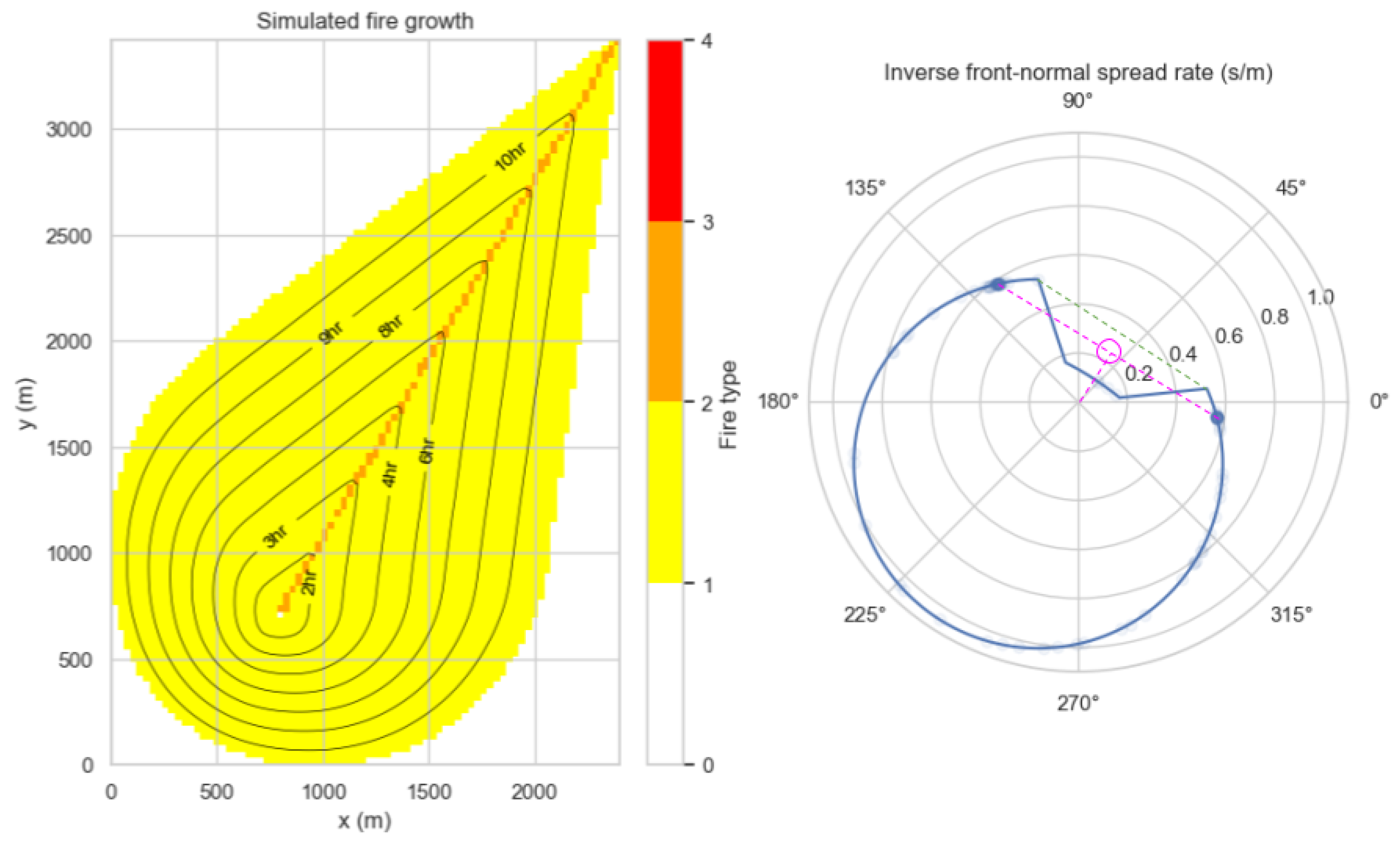
We now analyze the results of simulating speed-from-tangent models which violate the conditions of Proposition 1, which can happen in current fire spread models when there is crown fire. The right panel of Figure 9 displays in the conditions of experiment B1: we see a concavity in the heading fire direction, corresponding to an abrupt jump in spread rates from surface fire to active crown fire.
The left panel of Figure 9 shows the fire shapes yielded by the model in these conditions. We see an “arrowhead” pattern, leaving a thin trail of crown fire behavior. We find this behavior questionable for several reasons:
Figure 9.
Experiment B1: simulated fire growth from a non-smooth-growing model. The left panel shows the growth of the fire from a point ignition: contours represent time-of-arrival, and colors correspond to fire type (yellow for surface fire, orange for crown fire). The right panel displays the inverse front-normal spread rate function (blue curve): it is non-convex, which causes the fire perimeter to grow as a non-smooth “arrowhead” shape. The semi-transparent blue dots on top of the curve represent the spread rates observed at a random subset of burned pixels: we see two clusters corresponding to the front-normal direction at the flanks of the arrowhead. From these, the effective speed of the arrowhead can be deduced (purple circle). The correct shape and speed of the arrowhead (deduced from mathematical theory) are given by the dashed green line.
- 1.
- A substantive reason: only the pixels at the “tip” of the arrowhead experience crown fire; the rest consists of surface spread with the intensity of flanking or backing fire. In other words, there is virtually no heading fire. Also note that the effective speed of this arrowhead is lower than the heading crown fire spread rate. Qualitatively, these simulation results do agree with the theoretical behavior predicted by mathematical theory (Corollary 1 and Figure 6); our point here is that the theoretical model has disturbing implications.
- 2.
- A numerical reason: the effective speed of the arrowhead is faster than the theoretical speed determined by Corollary 1. In fact, the observed speed - and therefore the shape - of the arrowhead is a numerical artifact: it changes depending on the angle between the wind direction and the Cartesian grid, as shown by Figure 10.
Concretely, what happens during simulations is that Pyretechnics tries to resolve a front-normal direction in pixels that are close to the arrowhead tip; of course, this calculation is quite unstable and yields a distribution of spread rates - the effective speed of the arrowhead corresponds to the average effect of these numerical accidents. In our experiments, this effective speed is equal to the heading crown fire spread rate when the wind direction is grid-aligned, and is otherwise lower; of course, this is because Pyretechnics is a grid-based algorithm, and other algorithms can be expected to yield different behavior. Figure 11 will reveal that in all cases the arrowhead tip speed is overpredicted by simulations - it is always greater than the theoretical speed given by Proposition 2.
Optimistic readers might hope that the arrowhead sharpness is only due to starting the fire from a point ignition. Experiment B3 dispels this hope: Figure 11 shows a similar asymptotic pattern when the fire is started from a broad circular perimeter. We see that heading crown fire is initially present, but collapses into a pointed shape. This behavior is also predicted by theory (see Proposition 2 and Figure 6), although we observe that numerical errors cause simulations to mispredict even before the collapse is complete.
Figure 11.
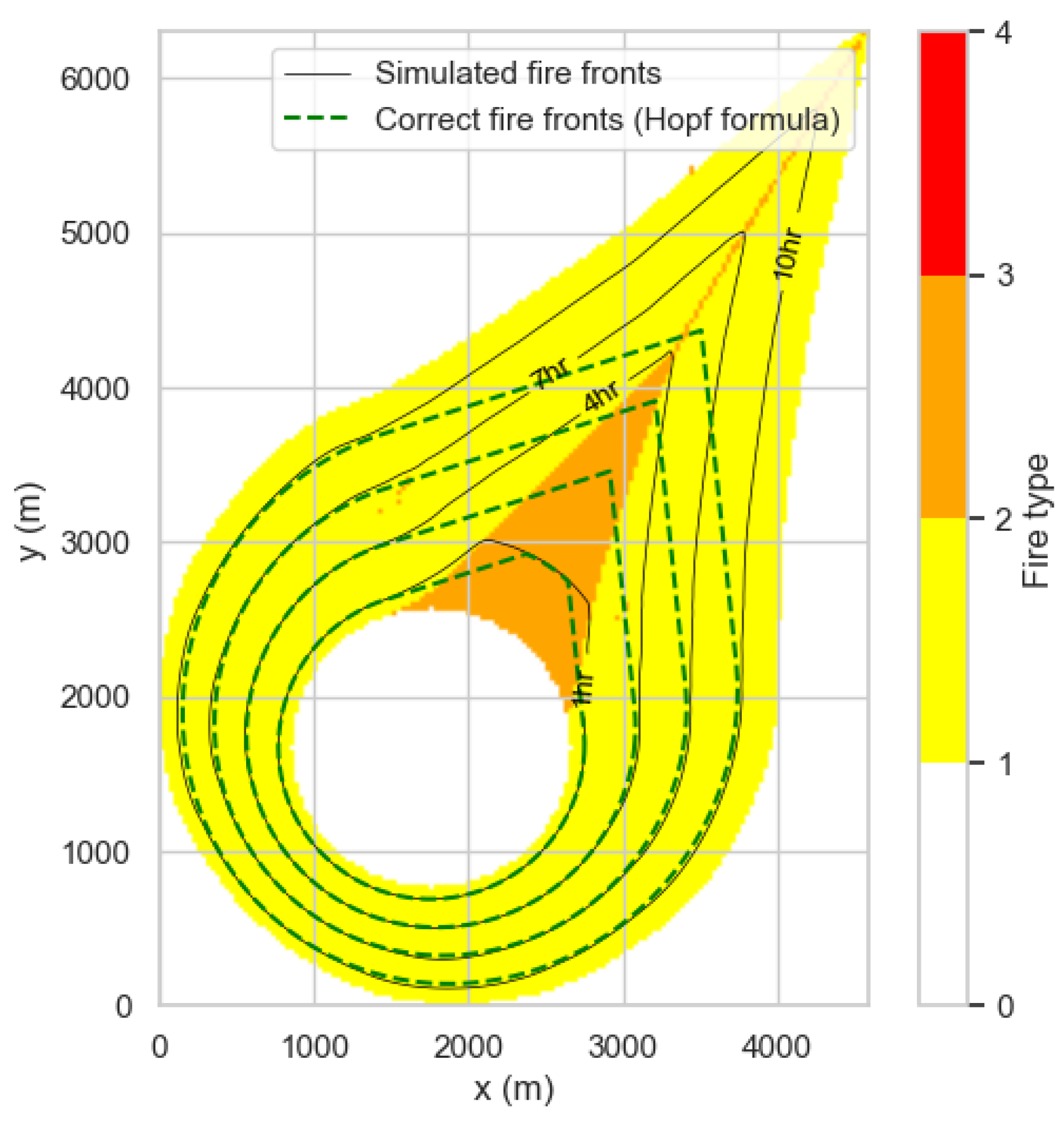
Fire growth in experiment B3, in which the initial perimeter is a broad circle. We see the heading crown fire collapsing into a pointed shape. Color shading represents the fire type (yellow for surface fire, orange for crown fire). Solid black lines are fire fronts obtained in simulations. Dashed green lines are fire fronts predicted from the mathematical theory developed in this paper, corresponding to the Hopf formula in Hamilton-Jacobi theory. We see that theory and simulations agree qualitatively but not quantitatively about the evolution of the fire - this is a symptom of numerical errors.
Figure 11.
Fire growth in experiment B3, in which the initial perimeter is a broad circle. We see the heading crown fire collapsing into a pointed shape. Color shading represents the fire type (yellow for surface fire, orange for crown fire). Solid black lines are fire fronts obtained in simulations. Dashed green lines are fire fronts predicted from the mathematical theory developed in this paper, corresponding to the Hopf formula in Hamilton-Jacobi theory. We see that theory and simulations agree qualitatively but not quantitatively about the evolution of the fire - this is a symptom of numerical errors.
Similarly, one might hope that fluctuations in wind direction might prevent crown fire collapse. This might help, but this is not always the case: Figure 12 shows examples where wind direction undergoes wide oscillations, but the collapse of heading crown fire is still observed - crown fire only occurs in short self-destructive bursts.
- An advanced remark: this too is something we could have anticipated from the theoretical results of Section 2.8. Wind fluctuations mean that the functions will “dig” concavities at various angles of the polar graph, if the wind direction doesn’t fluctuate too broadly the cumulative effect will be to dig roughly in the same direction, so that the integral of yields a persistent concavity which corresponds to a sharp tip in the fire perimeter.
Sharpness can happen in more varied ways than has been shown so far. Figure 13 shows the results of experiment B4, where concavities happen at the flanking direction due to a lower CBH, resulting in an earlier transition to crown fire. We see that this translates to sharp angles near the back of the fire perimeter, but heading crown fire is no longer collapsing. This arguably makes the presence of sharp angles much less concerning.
4. Discussion
We started this study by defining speed-from-tangent models (Section 2.2), Huygens wavelet models (Section 2.3), asking when they are equivalent, and in what conditions they preserve the smoothness of fire perimeters (Section 2.2.1). Section 2.5 has given all the answers: the models that preserve the smoothness of fire perimeters are exactly the Huygens wavelet models. Through the polar Legendre-Fenchel transform (Section 2.4), we also have learned that this is equivalent to a convexity criterion on the inverse spread rate function , and how to convert between spread rates and wavelet shapes. This equivalence result is a powerful motivation for Huygens wavelets as a modeling assumption: the Huygens principle is not as arbitrary as it might seem, because it arises naturally from an assumption of smoothness, which is a natural assumption to make as argued in Section 2.2.1 and [14].
In particular, the sharp wedge shapes observed in simulated crown fires (Figure 9, Figure 10, Figure 11, Figure 13) are not just numerical artefacts - they are an inevitable consequence of the discrete jump in spread rates at the threshold for crown fire. Indeed, this discrete jump induces a discontinuity in , and discontinuity prevents convexity; propositions 1 and 2 prove that these conditions make sharpness inevitable. To be clear: the presence of a wedge shape is inevitable, but the dimensions that it takes in simulations can easily be incorrect due to numerical errors, as revealed by experiment B2 (Figure 10).
Allowing for sharpness in predicted fire fronts causes two challenges:
- A theoretical challenge: the definition of the model is ambiguous, because the model is fundamentally describing how the perimeter is supposed to evolve in terms of its tangents, yet sharpness means that the tangent do not always exist. As described in Section 2.7, it seems that the best motivated approach consists of defining the model behavior as viscosity solutions to some partial differential equation (Eikonal or Hamilton-Jacobi).
- A numerical challenge: even after theoretical difficulties have been settled, experience shows that numerical algorithms can deviate massively from the theoretical behavior (Section 3).
The authors are concerned about several issues with models that create sharpness. We showed that some algorithms like Pyretechnics and FARSITE predict inaccurate and/or inconsistent fire shapes in these conditions, due to numerical errors. However, there is a deeper issue than numerical errors: it is not proven that such models are well-defined from a theoretical standpoint, i.e. they might yield inconsistent or ambiguous predictions. We made some progress by leveraging the notion of viscosity solution (Section 2.7), but the existence of viscosity solutions is still unclear to us when the initial burned region is not convex or when the conditions are not constant. Admittedly, this is the sort of problem that non-mathematicians are often content to treat as a non-issue.
Another concern is whether or not these pointed fire shapes are realistic. This question is not that easy to settle. Modelers might be tempted to decide that the smoothness of fire perimeters is a reasonable or even important assumption to make: this is indeed the assumption made in [14]. However, there are documented occurrences of real-world crown fires collapsing into pointed shapes, as reported in [23]:
Near its north western extent, the severity pattern of the western head formed a symmetric arrowhead pattern which several possible explanations acting separately or together (fig. 44). The first scenario results primarily from increasingly marginal conditions for supporting crown fire associated with nightfall. [...] The spread rate and intensity thresholds will become progressively limiting to the initiation and spread of crown fire from the flanks toward the head, resulting in a narrowing of the heading crown fire. The second scenario is suggested by the often-pointed shape of the head of some fast moving single-run crown fires attended by prolific spotting (for example, Sundance Fire in Idaho, Anderson 1968). A rapid change in the critical environmental conditions (for example, decreased winds or rain) could quickly terminate crown fire spread, leaving a footprint of high-severity effects to define the location of the crown fire at that time.
Thus, pointed shapes in crown fires might be a real phenomenon, and the present paper provides a theoretical explanation for them: “increasingly marginal conditions for supporting crown fire” might mean transitioning from Figure 13 to Figure 7, where the range of azimuths supporting crown fire becomes so narrow as to form a heading-fire concavity in the inverse spread rate profile, so that the heading fire self-destructs as in Figure 11. Of course, the similarity to these real-world fires might be superficial, and there might be competing explanations for these observations.
In particular, laboratory and field experiments have shown that pointed fire shapes can naturally occur in sloped terrain [39,40,41,42], due to convective feedbacks that create an indraft of convergent winds at the head of the fire, an effect which has been successfully simulated by coupled fire-atmosphere models [43]. We also note that the model of [44] approximates this effect through a fireline rotation model, which cannot be equivalent to a speed-from-tangent model, as it represents a cumulative effect on the wind field along the fire front. Generally speaking, non-coupled speed-from-tangent models probably cannot approximate convective feedbacks, because convective feedbacks create non-local effects on fire spread that act at characteristic length scales, whereas speed-from-tangent models are local and scale-invariant in nature. Thus, we have evidenced two completely different mechanisms that can lead to pointed fire shapes in real or simulated wildland fires: convective feedbacks as described in [43], and non-convex frontal kinetics as described in this paper. This leads us to the following recommendation: when observing pointed fire shapes, authors of coupled fire-atmosphere models should not conclude too readily that they successfully implemented convective feedbacks, as they might in fact be observing artefacts of their frontal speed parameterization.
The crown fire models we discussed here might be unrealistic in that they do not really model spread in the canopy layer: instead, they model a single front that encompasses both surface and crown fire, and re-evaluate whether crown fire occurs at each newly burned point, independently of how its surroundings were burned.
Head fire collapse means that simulated crown fires essentially have a self-destruct mechanism. Modelers who want to be conservative about crown fire risk might want to avoid this situation, lest the impact of crown fire be underestimated. Experiments C1 and C2 (Figure 12) showed that time-varying wind inputs alleviate the issue, as wind shifts rekindle flares of crown fire. Therefore, our findings speak against the common practice of using constant wind inputs in simulations.
One important question, which remains to be answered, is how frequently heading fire collapse can occur in real-world simulations with variable fuels and topography. We have learned from experiment B4 (Figure 13) and Section 2.7 that heading fire collapse can only happen when the transition to crown fire is close enough to the heading direction to shelter it in a concavity. How frequently that happens depends on the specifics of the crown fire model; in the one we used [3,16], it seems that this happens in a relatively narrow range of CBH values, outside which crown fire initiation happens either in almost all directions or none at all. Future work would do well to study this question more systematically.
At this point, it should also be clear that front propagation algorithms that are based on computing travel time along paths (such as cellular automata [10] and MTT [11]) are only applicable to smooth-growing models (Section 2.2.1), i.e. models that follow the Huygens principle and therefore satisfy the convexity criterion of Proposition 1. When that assumption is not met, the travel time along a path is not a well-defined quantity: this is apparent in Figure 11, where the speed along the heading direction is not the same before and after the heading fire collapse. When travel-time is a well-defined quantity, the region reachable from a point in unit time under constant conditions must be convex (to satisfy the triangle inequality), which implies a Huygens wavelet and therefore a smooth-growing model (see Section 2.3).
In summary, modelers have a dilemma: are sharp fire shapes a bug or a feature? The models that predict them have historically been based on real-world experiments and thoughtful assumptions [3], and as mentioned above they seem consistent some observed crown fire shapes. That being said, one should remember that these models are based on scant data: Van Wagner derived his seminal model based on 8 data points in conifer stands. On the other hand, this paper revealed some disturbing implications of these models: self-destroying heading fires which might underpredict crown fire prevalence, unproven well-definedness (in terms of existence and uniqueness of viscosity solutions in non-constant conditions, see Section 2.7), incompatibility with wavelet-based front-tracking methods like MTT [11] and cellular automata [10], and numerical challenges (Figure 10).
For modelers who deem that sharpness in simulated fires is undesirable, we can suggest the following low-cost correction:
- Decide whether crown fire initiation occurs based on the surface fire spread rate in the direction of fastest spread, instead of the front-normal direction.
- Compute the front-normal spread rate R as , where is the surface fire spread rate, and is the crown fire spread rate.
It is readily checked from Section 2.4 that this is equivalent to using a Huygens wavelet model with a wavelet shape that is the convex hull of the surface and crown wavelets merged together. We would then get fire shapes similar to Figure 8, in which the flanks feature straight line segments corresponding to the sharp (i.e. continuous but not differentiable) transition between surface and crown fire spread rate. Note that this would create a dilemma in terms of predicted fire behavior: are these flanks burning as surface or crown fire? The answer is unclear as these flanks correspond exactly to the front-normal direction of transition. That said, non-constant inputs might make the question moot in practice.
On the other hand, modelers who find sharpness desirable should at least address the numerical challenges. When using the level-set method, this might be achieved by adding a regularization term to the Hamilton-Jacobi equation (equation 34) to account for curvature, as exemplified by [34] who added a viscosity term to the Hamiltonian. Viscosity solutions are often characterized as the limit of such equations as the viscosity term becomes negligible [17], therefore we expect that the large-scale fire shapes predicted by this approach will agree with the viscosity solutions we described in Section 2.7. We also note that other approaches to fire spread modeling have used more sophisticated partial differential equations for modeling the fire front, such as reaction-diffusion equations and the KPZ class of equations [5,6,45].
Let us relate the methods of this paper to other scientific fields. Propagating fire with the Huygens principle corresponds to the case where the convexity criterion of Proposition 1 is respected. This is equivalent to a convex Hamiltonian in the corresponding Eikonal and Hamilton-Jacobi equations (Equation 20 and 34). Then, the Hamiltonian is the Legendre-Fenchel transform of the Lagrangian, and fire spread is naturally modeled through the lens of the Minimal-Travel-Time trajectories, where the Lagrangian is used to measure travel time. The duality between fronts and trajectories corresponds to the duality between rays and waves in optics, the domain in which both the Huygens principle and the Eikonal equation were originally formulated. When conditions are spatially varying, this can be theorized in several equivalent ways: as the method of characteristics [17] for the corresponding Hamilton-Jacobi equation, and also through the notion of Finsler spaces and Randers geodesics, which have been related to wildfire spread models in [46,47,48]. We saw that in constant conditions the Huygens principle was equivalent to a convolution (Section 2.6); this convolution corresponds to dilation in the field of mathematical morphology: see [49] for the connection to Hamilton-Jacobi theory. Much of the Hamilton-Jacobi literature assumes that the Hamiltonian is convex. One notable exception is the field of differential game theory [50], in which non-convex Hamiltonians arise in the Hamilton-Jacobi equation. Crystallography is another field where convexity violations lead to sharp shapes [51]; most of the partial differential equations studied in this context involve second-order curvature terms, and therefore are not directly applicable to speed-from-tangent fire spread models; however, the kinetic Wulff construction seems particularly relatable to the present paper [52]. Exploring these connections from a wildfire perspective might be fruitful directions for future work.
Skeptical readers might have doubts about the validity of our mathematical results, in particular because our polar Hopf formula (Proposition 2) predicts surprisingly small and slow fires: could it be that the mathematical proofs in this paper contain errors that survived peer review, or maybe that viscosity solutions (Section 2.7) are an artificial mathematical assumption? We emphasize that these results are corroborated by much more than the math of the present paper:
- 1.
- The classical Hopf formula [31,35] is one of the most established results from Hamilton-Jacobi theory (see Section 2.7.6), and predicts the same fire perimeters as Proposition 2.
- 2.
- The simple and intuitive principle that making the initial perimeter larger should make the final perimeter no smaller. Arguably, even readers who (quite eccentrically) do not believe in viscosity solutions will at least agree with this principle. By considering the half-planes that contain the initial perimeter, it becomes clear that the final perimeter predicted by Proposition 2 is the largest final perimeter allowed by this principle.
We stress that the methods developed in this paper can be useful beyond the thorny issue of crown fires. We have seen how the polar Legendre-Fenchel transform (Section 2.4) can shed light on the duality between fire shapes and spread rates, which can be useful to guide the design of fire spread models. Furthermore, we now have broadly applicable analytical formulas to exactly predict fire growth in spatially constant conditions, even when they vary in time (Section 2.8). Even though spatially constant conditions are not realistic, these formulas provide advanced ways to assess the accuracy of simulation algorithms. More precisely, these formulas are applicable when either one of the following conditions is met:
- 1.
- the initial burned region is convex (Propositions 2 and 6), or
- 2.
- the model is smooth-growing (Equation 14 and Proposition 5), i.e. satisfies the conditions of Proposition 1.
5. Conclusions
In summary: we have improved our understanding of a broad class of wildfire growth models, by developing a mathematical framework that solves the fire spread equations in more generality than previously done in the fire modeling literature. In particular, this explains the emergence of sharpness in modeled fire fronts.
More precisely, we set out to document and study the phenomenon of simulated crown fires collapsing into sharp pointed shapes. Our study is in the context of what we call speed-from-tangent models, which are defined by specifying the rate of spread normal to the fire front as a function of the local conditions (weather, fuels, slope) and the orientation of the fire front. We showed that preserving the smoothness of fire fronts is equivalent to a convexity criterion on the inverse spread rate function, and that this criterion is also equivalent to following Huygens’ Principle. We also learned that convex duality (namely, the Legendre-Fenchel transform) is instrumental to converting between the Huygens wavelet shape and the (inverse) spread rate function.
Allowing for sharpness may or may not be desirable, and we discussed that issue. We see some features of real-world crown fires which suggest that sharpness might be realistic. However, sharpness causes challenges in making the models well-defined, which we partially addressed by reframing the problem as finding viscosity solutions to a partial differential equation. Sharpness also causes numerical challenges.
The above findings were achieved by deriving exact analytical formulas for predicting the fire perimeter in spatially constant conditions, applicable when the model respects the convexity criterion or when the initial burned region is convex. These formulas can be used for verification of numerical fire spread algorithms.
Author Contributions
Conceptualization, V.W.; methodology, V.W.; software, V.W.; validation, V.W. and D.S.; formal analysis, V.W.; investigation, V.W.; resources, D.S.; data curation, V.W.; writing—original draft preparation, V.W.; writing—review and editing, V.W. and D.S.; visualization, V.W.; supervision, D.S.; project administration, D.S.; funding acquisition, D.S. All authors have read and agreed to the published version of the manuscript.
Funding
This research received no external funding.
Data Availability Statement
Not applicable.
Acknowledgments
The authors thank Mark Finney, Antonin de Courcel, Arthur Loison, Antonin Chambolle, Gary Johnson, Kayla Johnston, Scott Ritter, David Schmidt, Dawn Nekorchuk, Pauline Vialatte, Carrie Levine, and Teal Richards-Dimitrie for supporting this work.
Conflicts of Interest
The authors declare no conflicts of interest.
Abbreviations
The following abbreviations are used in this manuscript:
| CBH | Canopy base height |
| CBD | Crown bulk density |
| ToA | Time of Arrival |
| MTT | Minimal Travel Time |
| MDPI | Multidisciplinary Digital Publishing Institute |
References
- Oliveira, S.; Rocha, J.; Sá, A. Wildfire risk modeling. Current Opinion in Environmental Science & Health 2021, 23, 100274. [Google Scholar] [CrossRef]
- Silva, J.; Marques, J.; Gonçalves, I.; Brito, R.; Teixeira, S.; Teixeira, J.; Alvelos, F. A Systematic Review and Bibliometric Analysis of Wildland Fire Behavior Modeling. Fluids 2022, 7, 374. [Google Scholar] [CrossRef]
- Wagner, C.E.V. Conditions for the start and spread of crown fire. Canadian Journal of Forest Research 1977, 7, 23–34. [Google Scholar] [CrossRef]
- Majda, A.J.; Souganidis, P.E. Large scale front dynamics for turbulent reaction-diffusion equations with separated velocity scales. Nonlinearity 1994, 7, 1. [Google Scholar] [CrossRef]
- Séro-Guillaume, O.; Ramezani, S.; Margerit, J.; Calogine, D. On large scale forest fires propagation models. International Journal of Thermal Sciences 2008, 47, 680–694. [Google Scholar] [CrossRef]
- Grasso, P.; Innocente, M. A two-dimensional reaction-advection-diffusion model of the spread of fire in wildlands. In Advances in Forest Fire Research 2018; Imprensa da Universidade de Coimbra, 2018; pp. 334–342. [Google Scholar]
- Finney, M.A. FARSITE, Fire Area Simulator–model development and evaluation; The Station, 2004. [Google Scholar]
- Anderson, D.; Catchpole, E.; De Mestre, N.; Parkes, T. Modelling the spread of grass fires. The ANZIAM Journal 1982, 23, 451–466. [Google Scholar] [CrossRef]
- Knight, I.; Coleman, J. A fire perimeter expansion algorithm-based on Huygens wavelet propagation. International Journal of Wildland Fire 1993, 3, 73–84. [Google Scholar] [CrossRef]
- Clarke, K.C.; Brass, J.A.; Riggan, P.J. A cellular automaton model of wildfire propagation and extinction. Photogrammetric Engineering and Remote Sensing 1994, 60((11) 60), 1355-1367 1355–1367. [Google Scholar]
- Finney, M.A. Fire growth using minimum travel time methods. Canadian Journal of Forest Research 2002, 32, 1420–1424. [Google Scholar] [CrossRef]
- Rehm, R.G.; McDermott, R.J. Fire-front propagation using the level set method; US Department of Commerce, National Institute of Standards and Technology …, 2009. [Google Scholar]
- Lautenberger, C. Wildland fire modeling with an Eulerian level set method and automated calibration. Fire Safety Journal 2013, 62, 289–298. [Google Scholar] [CrossRef]
- Richards, G.D. A general mathematical framework for modeling two-dimensional wildland fire spread. International Journal of Wildland Fire 1995, 5, 63–72. [Google Scholar] [CrossRef]
- Rockafellar, R.T. Convex analysis:(pms-28). 2015. [Google Scholar]
- Cruz, M.G.; Alexander, M.E.; Wakimoto, R.H. Development and testing of models for predicting crown fire rate of spread in conifer forest stands. Canadian Journal of Forest Research 2005, 35, 1626–1639. [Google Scholar] [CrossRef]
- Evans, L.C. Partial differential equations; American mathematical society, 2022; Vol. 19. [Google Scholar]
- Koike, S. A beginner’s guide to the theory of viscosity solutions. In MSJ Mem.; 2004. [Google Scholar]
- Crandall, M.G.; Lions, P.L. Viscosity solutions of Hamilton-Jacobi equations. Transactions of the American mathematical society 1983, 277, 1–42. [Google Scholar] [CrossRef]
- Barles, G. Remarks on a flame propagation model. PhD thesis, INRIA, 1985. [Google Scholar]
- Sethian, J.A. An analysis of flame propagation; University of California: Berkeley, 1982. [Google Scholar]
- Lautenberger, C. ELMFIRE Verification Case 01: Elliptical fire shape. https://elmfire.io/verification/verification_01.html, 2023. Accessed: 2025-09-03.
- Graham, R.T. Hayman fire case study; US Department of Agriculture, Forest Service, Rocky Mountain Research Station, 2003. [Google Scholar]
- Tiel, J.v. Convex analysis: an introductory text. No Title 1984. [Google Scholar]
- Tymstra, C.; Bryce, R.; Wotton, B.; Taylor, S.; Armitage, O.; et al. Natural Resources Canada, Canadian Forest Service, Northern Forestry Centre, Information Report NOR-X-417; Development and structure of Prometheus: the Canadian wildland fire growth simulation model. Edmonton, AB, 2010.
- Johnson, G.W.; Waeselynck, V.; Lautenberger, C.; Saah, D. Pyretechnics API documentation. https://pyregence.github.io/pyretechnics/, 2024. Accessed: 2025-09-03.
- Andrews, P.L. The Rothermel surface fire spread model and associated developments: a comprehensive explanation; 2018. [Google Scholar]
- Rothermel, R.C. A mathematical model for predicting fire spread in wildland fuels. In Research paper/Intermountain forest and range experiment station; USDA (INT-115), 1972. [Google Scholar]
- Byram, G.M. Combustion of forest fuels. Forest fire: Control and use 1959, 1, 61–89. [Google Scholar]
- Touchette, H. Legendre-Fenchel transforms in a nutshell. URL http://www. maths. qmul. ac. uk/ht/archive/lfth2. pdf 2005, p. 25.
- Hopf, E. Generalized solutions of non-linear equations of first order. Journal of Mathematics and Mechanics 1965, 14, 951–973. [Google Scholar]
- Giga, Y. Surface evolution equations: a level set method. Hokkaido University technical report series in mathematics 2002, 71, 1. [Google Scholar]
- Osher, S.; Fedkiw, R.; Piechor, K. Level set methods and dynamic implicit surfaces. Appl. Mech. Rev. 2004, 57, B15–B15. [Google Scholar] [CrossRef]
- Muñoz-Esparza, D.; Kosović, B.; Jiménez, P.A.; Coen, J.L. An accurate fire-spread algorithm in the Weather Research and Forecasting model using the level-set method. Journal of Advances in Modeling Earth Systems 2018, 10, 908–926. [Google Scholar] [CrossRef]
- Evans, L.C. Envelopes and nonconvex Hamilton–Jacobi equations. Calculus of Variations and Partial Differential Equations 2014, 50, 257–282. [Google Scholar] [CrossRef]
- Barles, G. Uniqueness for first-order Hamilton-Jacobi equations and Hopf formula. Journal of differential equations 1987, 69, 346–367. [Google Scholar] [CrossRef]
- Heinsch, F.A.; Andrews, P.L. BehavePlus fire modeling system, version 5.0: design and features. Gen. Tech. Rep. RMRS-GTR-249. US Department of Agriculture, Forest Service, Rocky Mountain Research Station: Fort Collins, CO, 2010; 249. [Google Scholar]
- Williams, C.K.; Rasmussen, C.E. Gaussian processes for machine learning; MIT: Cambridge, MA, 2006; Vol. 2. [Google Scholar]
- Dupuy, J.L.; Maréchal, J.; Portier, D.; Valette, J.C. The effects of slope and fuel bed width on laboratory fire behaviour. International Journal of Wildland Fire 2011, 20, 272–288. [Google Scholar] [CrossRef]
- Silvani, X.; Morandini, F.; Dupuy, J.L. Effects of slope on fire spread observed through video images and multiple-point thermal measurements. Experimental Thermal and Fluid Science 2012, 41, 99–111. [Google Scholar] [CrossRef]
- Viegas, D.X. Fire line rotation as a mechanism for fire spread on a uniform slope. International Journal of Wildland Fire 2002, 11, 11–23. [Google Scholar] [CrossRef]
- Cheney, N.P.; Gould, J.S. Fire growth in grassland fuels. International Journal of Wildland Fire 1995, 5, 237–247. [Google Scholar] [CrossRef]
- Clark, T.L.; Jenkins, M.A.; Coen, J.; Packham, D. A coupled atmosphere fire model: Convective feedback on fire-line dynamics. Journal of Applied Meteorology and Climatology 1996, 35, 875–901. [Google Scholar] [CrossRef]
- Viegas, D.X.; Ribeiro, C.; Barbosa, T.F.; Rodrigues, T.; Ribeiro, L.M. A Fireline Displacement Model to Predict Fire Spread. Fire 2024, 7, 121. [Google Scholar] [CrossRef]
- Provatas, N.; Ala-Nissila, T.; Grant, M.; Elder, K.; Piché, L. Scaling, propagation, and kinetic roughening of flame fronts in random media. Journal of statistical physics 1995, 81, 737–759. [Google Scholar] [CrossRef]
- Dehkordi, H.R. Applications of Randers geodesics for wildfire spread modelling. Applied Mathematical Modelling 2022, 106, 45–59. [Google Scholar] [CrossRef]
- Monedero, S.; Ramírez, J.; Molina-Terrén, D.; Cardil, A. Simulating wildfires backwards in time from the final fire perimeter in point-functional fire models. Environmental Modelling & Software 2017, 92, 163–168. [Google Scholar] [CrossRef]
- Dehkordi, H.R. On the paths through which the fire progress faster. Proceeding Series of the Brazilian Society of Computational and Applied Mathematics, 2022; 9. [Google Scholar]
- Arehart, A.B.; Vincent, L.; Kimia, B.B. Mathematical morphology: The hamilton-jacobi connection. In Proceedings of the 1993 (4th) International Conference on Computer Vision. IEEE, 1993; pp. 215–219. [Google Scholar]
- Pierre, C. Introduction to differential games. In Universite de Brest, Place du Marchal De Lattre De Tassigny; 2010; Volume 75775. [Google Scholar]
- Angenent, S.; Gurtin, M.E. Multiphase thermomechanics with interfacial structure 2. Evolution of an isothermal interface. Archive for Rational Mechanics and Analysis 1989, 108, 323–391. [Google Scholar] [CrossRef]
- Sekerka, R.F. Equilibrium and growth shapes of crystals: how do they differ and why should we care? Crystal Research and Technology: Journal of Experimental and Industrial Crystallography 2005, 40, 291–306. [Google Scholar] [CrossRef]
Figure 1.
Polar plots of functions which are respectively (a) polar-convex, and (b) not polar-convex, having a concavity at 315°. The radial graph of each function (defined as the region ) is filled with semi-transparent blue shading. We call a function polar-convex if and only if its radial graph is convex.
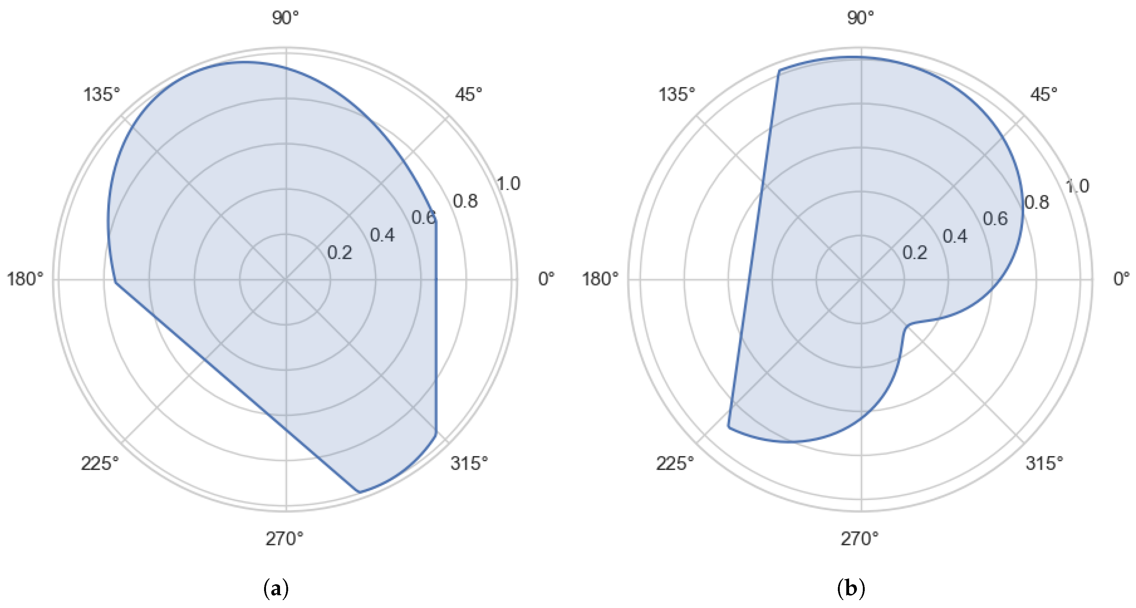
Figure 2.
Schematic illustration of the front-normal spread rate . is an azimuth indicating the direction normal to the fire front. During infinitesimal time , the fire front advances a distance . Here is assumed to be sufficiently small that the section of fire front can be approximated as a straight line.
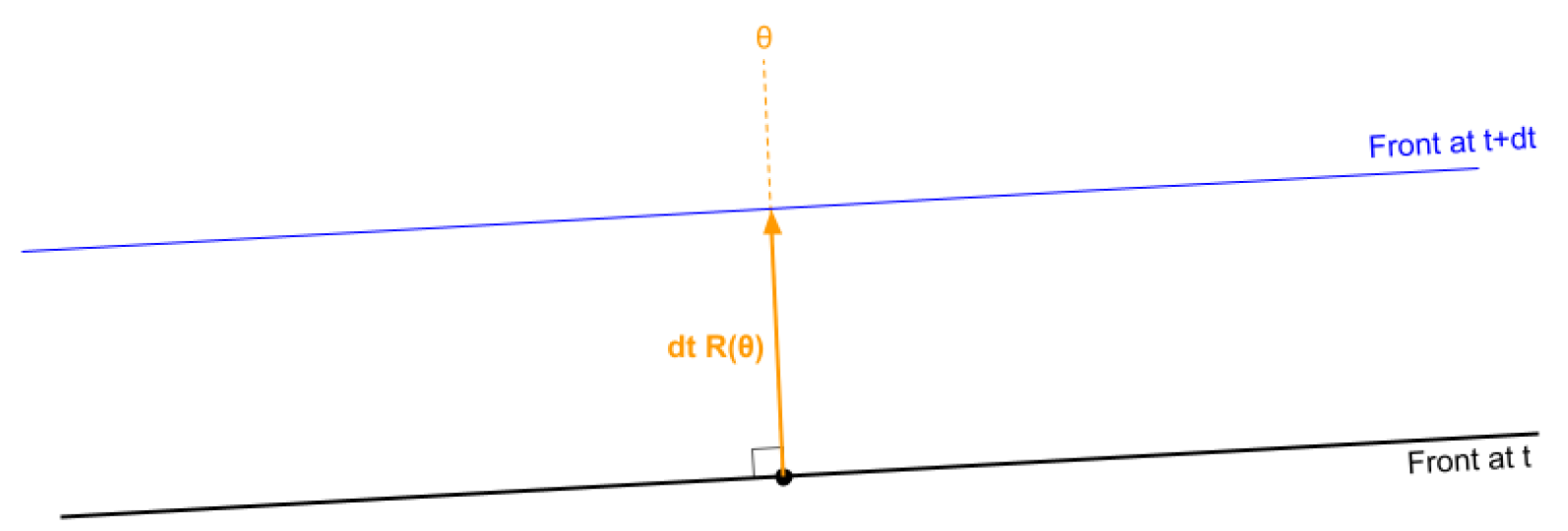
Figure 3.
Illustration of front propagation using the Huygens principle. The solid and dashed orange lines represent the fire front at times t and , respectively. the blue ellipses represent the duration- wavelets.
Figure 3.
Illustration of front propagation using the Huygens principle. The solid and dashed orange lines represent the fire front at times t and , respectively. the blue ellipses represent the duration- wavelets.
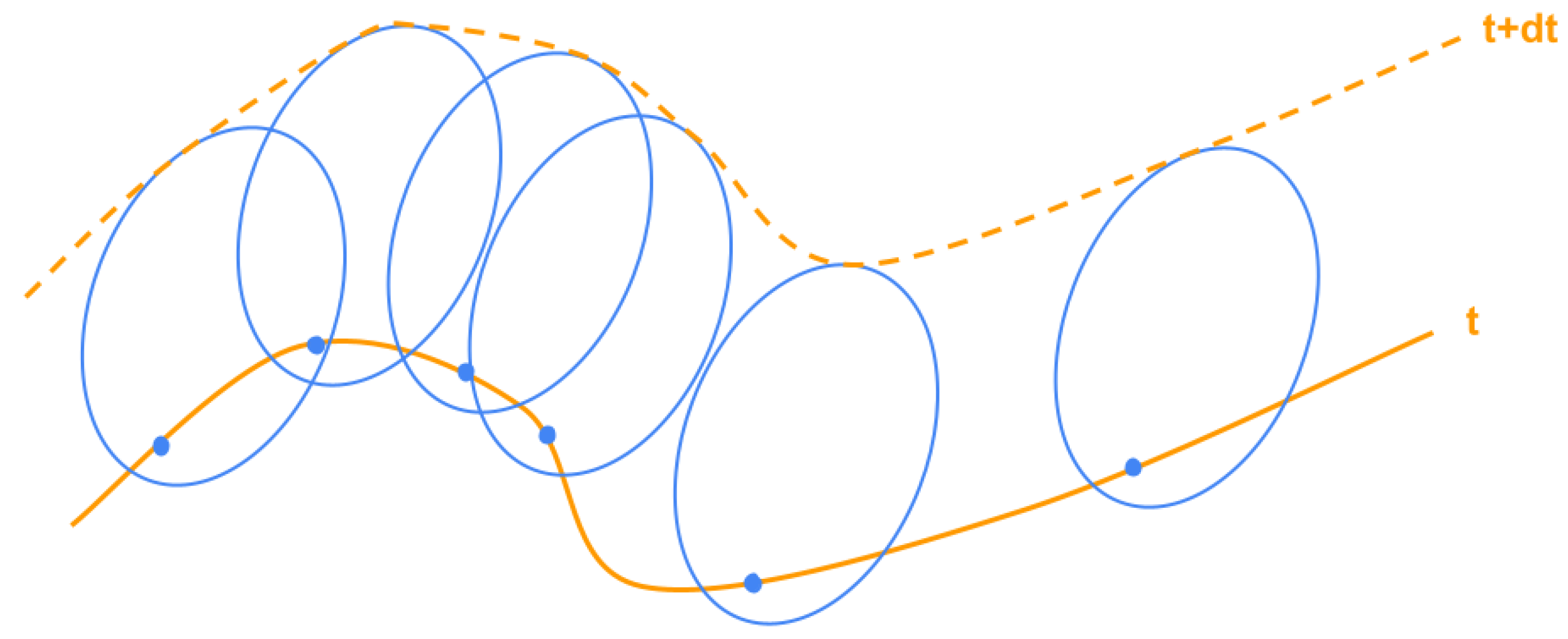
Figure 4.
Illustration of the geometric relation between (the front-normal spread rate in direction ) and (the Huygens wavelet speed in other directions).
Figure 4.
Illustration of the geometric relation between (the front-normal spread rate in direction ) and (the Huygens wavelet speed in other directions).
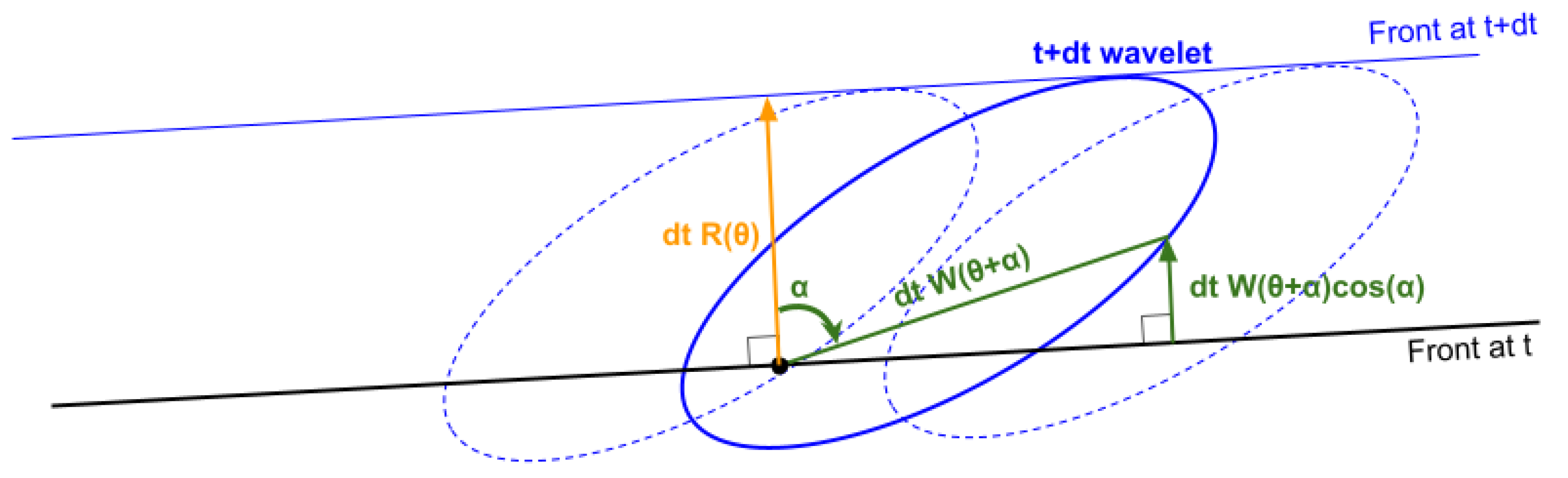
Figure 5.
Illustration of how the wavelet shape can be recovered from the front-normal spread rate in other directions . The main geometric idea is that a convex shape can be reconstructed from its supporting lines.
Figure 5.
Illustration of how the wavelet shape can be recovered from the front-normal spread rate in other directions . The main geometric idea is that a convex shape can be reconstructed from its supporting lines.
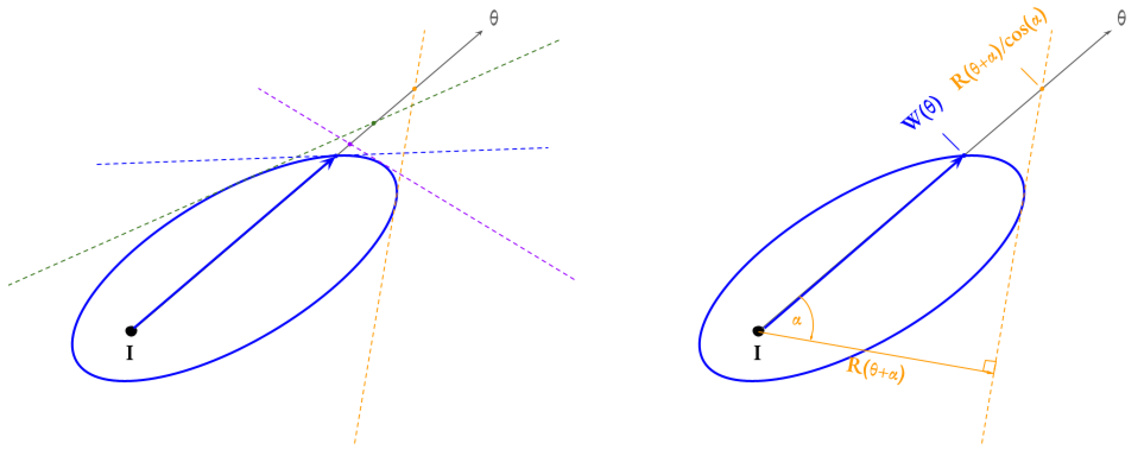
Figure 7.
Inverse front-normal spread rate profile yielded by the default simulation inputs used in this paper. The downwind direction is 57°. We see a concavity caused by a sharp increase in spread rate, due to the transition between surface and crown fire. Note that the straight lines directed towards the origin represent discrete discontinuous jumps in inverse spread rates, not linear variations - the function is discontinuous at these angles, despite what the plotting method might suggest. Inside the concavity, the crown fire inverse spread rates describe a circular arc about 100° wide, of very small length because crown fire spread rates are very high.
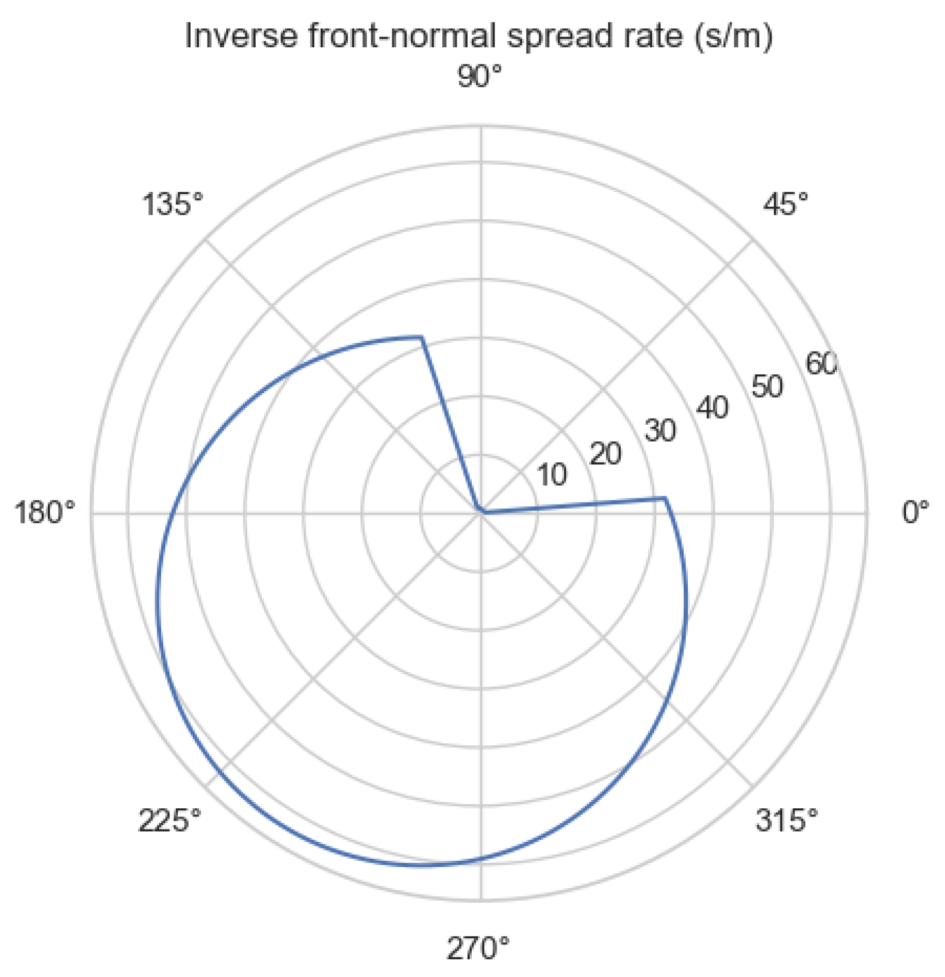
Figure 8.
Comparing simulated and predicted 24-hr fire perimeters, in homogeneous conditions that yield some smooth-growing crown fire with nontrivial perimeter shapes. The solid orange line was obtained by simulating a fire from the point of ignition, and drawing the 24-hr contour of the output Time-of-Arrival map. The dashed blue line represents the perimeter predicted by the mathematical theory developed in the present paper; it was obtained by resolving the inverse front-normal spread rate in all directions (right panel), then computing the polar Legendre-Fenchel transform. Fuels and weather inputs were chosen to ensure that the shape plotted in the right panel is convex, which ensures that the model is smooth-growing despite the presence of crown fire.
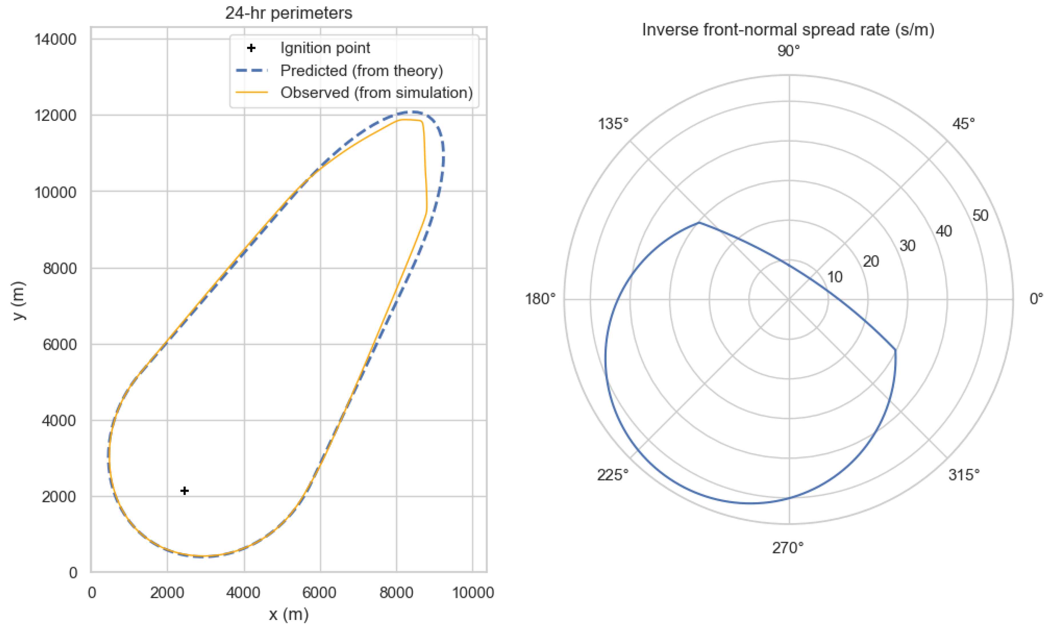
Figure 10.
10-hr fire perimeters in simulated experiment B2, for various wind directions. The fires used the same inputs except for the wind direction. This reveals that the simulated fire shapes are representative of numerical accidents rather than the underlying continuous model.
Figure 10.
10-hr fire perimeters in simulated experiment B2, for various wind directions. The fires used the same inputs except for the wind direction. This reveals that the simulated fire shapes are representative of numerical accidents rather than the underlying continuous model.
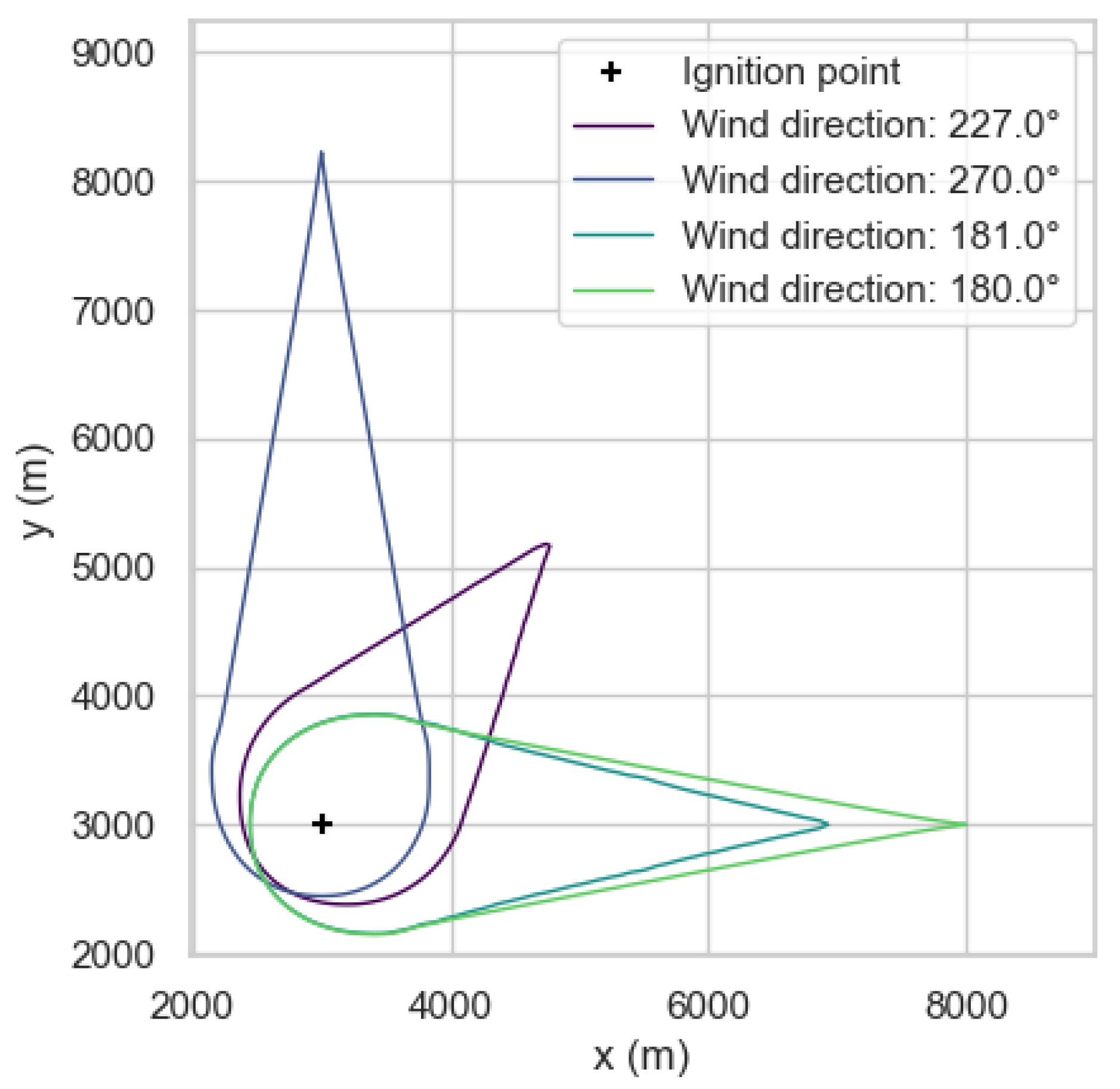
Figure 12.
Simulated fire perimeters in experiment C, featuring fluctuations in wind direction (a) as a sine wave, and (b) as a random Gaussian process with a Matérn (5/2) covariance kernel and a length scale of 2 hours. Contours represent the fire perimeters at various time since ignitions. The colors represent fire type: yellow means surface fire, and red means active crown fire.
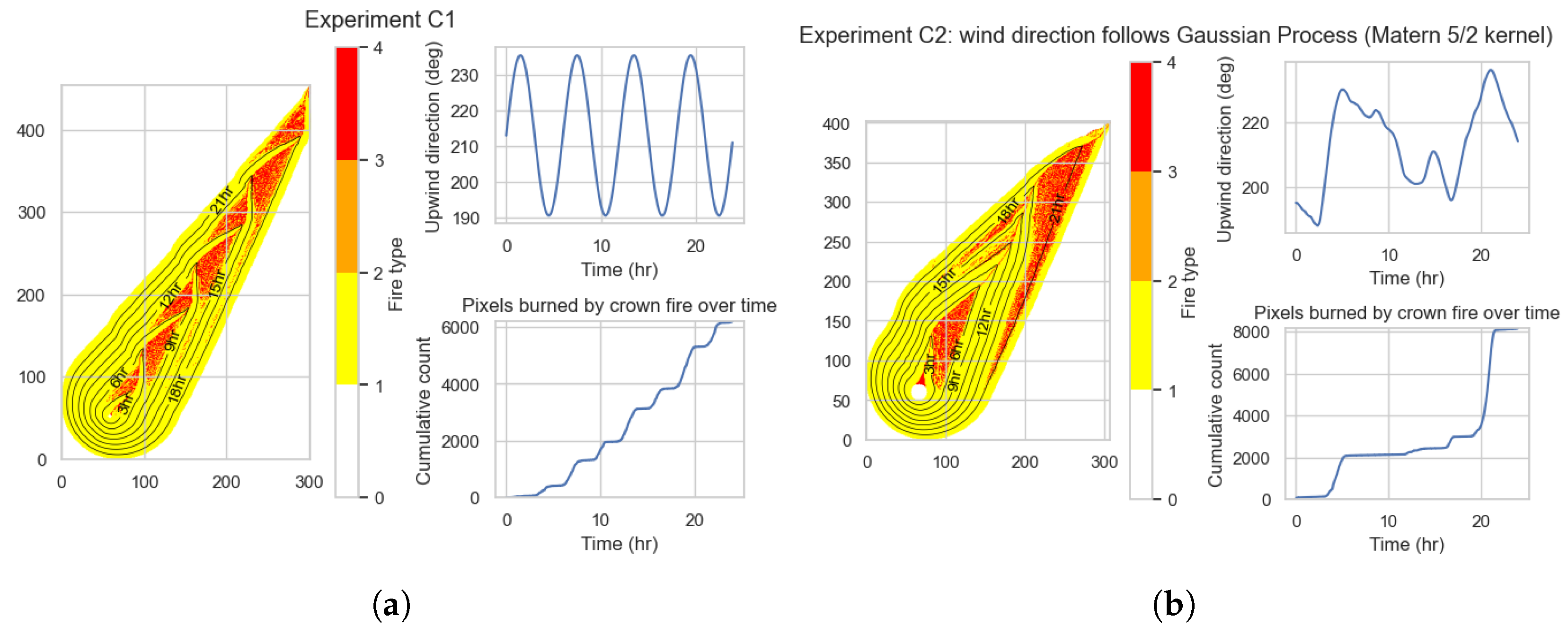
Figure 13.
Fire growth in experiment B4. In the left panel, contours represent time-of-arrival, and colors correspond to fire type (yellow for surface fire, orange and red for passive and active crown fire). The low CBH value causes transition to crown fire to happen in the backing fire directions (see right panel). This yields a “keyhole” shape in the inverse front-normal spread rate profile (right panel), where concavities happen at the flanks. These concavities translate to sharp angles near the back of the predicted fire perimeter.
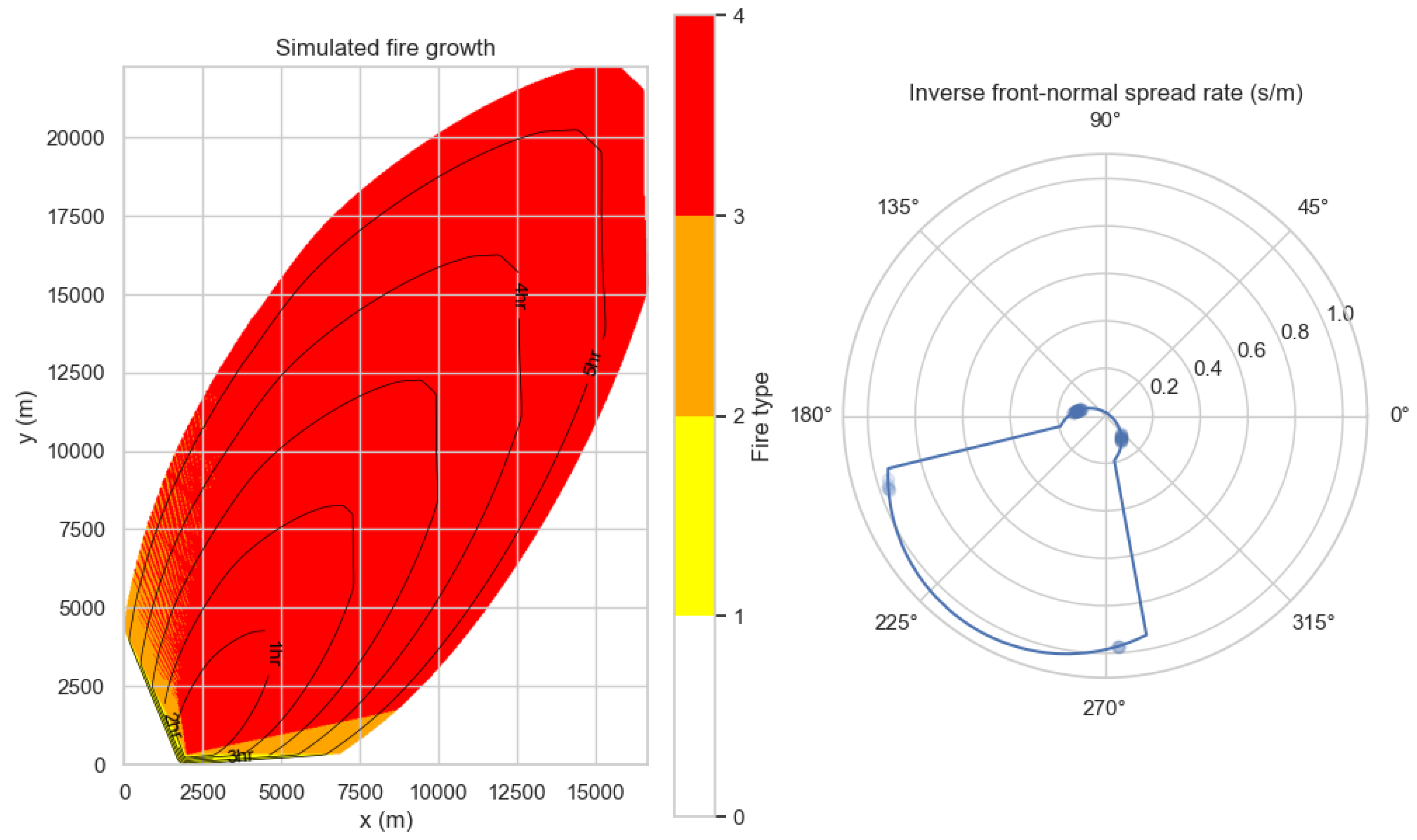

Table 1.
Main notation used in this paper. denotes the unit of quantity Q; if Q is a function, denotes the unit of the function’s output values.
Table 1.
Main notation used in this paper. denotes the unit of quantity Q; if Q is a function, denotes the unit of the function’s output values.
| Symbol | Unit | Meaning |
|---|---|---|
| rad | Azimuth (i.e. angle indicating a direction) | |
| m/s | Front-normal spread rate (Section 2.2) | |
| m/s | Huygens wavelet radial speed (Section 2.3) | |
| t | s | Time since ignition |
| s | Infinitesimal time increment | |
| m | Perimeter (fire front) at time t | |
| - | Burned region at time t (set of 2D vectors) | |
| - | Supremum (≈ “maximum”) of a set A of real numbers | |
| - | Infimum (≈ “minimum”) of a set A of real numbers | |
| Polar Legendre-Fenchel transform of f (Section 2.4) | ||
| - | (Polar) convolution of and (Section 2.6) | |
| Magnitude of a vector | ||
| Dot product of vectors and | ||
| m | Position in the plane (2D vector) | |
| s/m | Inverse spread rate vector (2D vector) | |
| s | Time-of-Arrival (ToA) function | |
| Partial derivative of function f with respect to z | ||
| s/m | Spatial gradient of (2D vector) | |
| (or ) | - | Hamiltonian function (Section 2.7.2) |
| - | (front-normal) unit vector (2D vector) | |
| - | Indicator function of a set S (Equation 23) | |
| Convex conjugate of f (Equation 22) |
Table 2.
Default inputs used in the fire spread simulation experiments of this paper. Fuel moistures are ratios of water content weight divided by oven-dry weight. Directional inputs are in degrees counterclockwise from east.
Table 2.
Default inputs used in the fire spread simulation experiments of this paper. Fuel moistures are ratios of water content weight divided by oven-dry weight. Directional inputs are in degrees counterclockwise from east.
| Input variable | Unit | Value |
|---|---|---|
| Slope | rise/run | 0 |
| Aspect | ° | 0 |
| Fuel model number | Categorical | 203 |
| Canopy cover | fraction | 0.7 |
| Canopy height | m | 10 |
| Canopy base height (CBH) | m | 2.5 |
| Crown bulk density (CBD) | 0.3 | |
| 10 m wind speed | 5.56 | |
| Upwind direction | ° | 237 |
| 1hr fuel moisture | fraction | 0.03 |
| 10hr fuel moisture | fraction | 0.04 |
| 100hr fuel moisture | fraction | 0.05 |
| Herbaceous fuel moisture | fraction | 0.90 |
| Woody fuel moisture | fraction | 0.60 |
| Foliar moisture | fraction | 0.90 |
| Temperature | °C | 30 |
Disclaimer/Publisher’s Note: The statements, opinions and data contained in all publications are solely those of the individual author(s) and contributor(s) and not of MDPI and/or the editor(s). MDPI and/or the editor(s) disclaim responsibility for any injury to people or property resulting from any ideas, methods, instructions or products referred to in the content. |
© 2026 by the authors. Licensee MDPI, Basel, Switzerland. This article is an open access article distributed under the terms and conditions of the Creative Commons Attribution (CC BY) license (http://creativecommons.org/licenses/by/4.0/).
Copyright: This open access article is published under a Creative Commons CC BY 4.0 license, which permit the free download, distribution, and reuse, provided that the author and preprint are cited in any reuse.


