Submitted:
10 February 2026
Posted:
11 February 2026
You are already at the latest version
Abstract
Livestock grazing strongly influences terrestrial ecosystems and plays a critical role in carbon dynamics, with outcomes highly dependent on grazing management. High-frequency rotation (HFR) grazing has been proposed to reduce the uneven spatial grazing distribution commonly associated with low-frequency rotation (LFR) grazing, potentially altering forage production and soil organic carbon (SOC). However, most ecosystem models used to assess SOC dynamics do not explicitly represent uneven grazing distribution, limiting their ability to evaluate management effects. To address this limitation, we enhanced the MEMS ecosystem model by incorporating a spatially explicit grazing distribution through the introduction of discrete spatial units and key environmental drivers, including forage availability and quality, and distance to water. Using remote sensing-derived enhanced vegetation index (EVI), we verified the simulated grazing distribution using an experimental rangeland site in Oklahoma. We tested the model’s sensitivity to grazing frequency under different management (stocking rate, timing, and duration) and climate (typical, dry, and wet) scenarios. Our results indicate that uneven grazing distribution leads to distinct spatial patterns of forage production and SOC. Notably, significant differences in field-average production and SOC between HFR and LFR emerged under heavy intensity grazing, where HFR sustained higher SOC stocks and productivity than LFR. These findings highlight the importance of spatially explicit modeling in understanding grazing distributions, suggesting that HFR grazing may be beneficial mostly under heavy intensity grazing. Our study offers actionable guidance for designing future grazing management experiments to address this critical knowledge gap and advance carbon management strategies.
Keywords:
ecosystem model
; soil organic carbon
; rotational grazing
; forage production
1. Introduction
Grazing lands, including both pastures and rangelands, are among the most widespread land uses on Earth, covering ~67% of the agricultural land [1]. They are estimated to store between 10-30% of global soil organic carbon (SOC) stocks, with management playing a crucial role in shaping SOC dynamics [2,3]. Historically, most grazing lands have been poorly managed, leading to land degradation and significant SOC losses [4,5]. Improving grazing management strategies offers an opportunity to recover and enhance SOC storage, while mitigating climate change [6]. Globally, it is estimated that adopting improved grazing practices could result in SOC sequestration potential ranging from 148 to 699 megatons of carbon dioxide equivalents per year [2].
Effective grazing management strategies involve manipulating key levers, such as grazing frequency, duration, stocking density, and timing [7]. Among these strategies, high-frequency rotation (HFR) grazing management, characterized by daily or sub-daily movement of livestock across small paddocks with high stocking density, has gained popularity in recent years and has been shown to potentially enhance SOC storage [8,9,10,11,12,13]. This intensive approach promotes more uniform grazing across the landscape, reducing both under and overgrazing in localized areas [14,15,16]. Conversely, low-frequency rotation (LFR) management, where animals graze larger areas for extended periods, often results in uneven grazing patterns. Under this management, livestock tend to concentrate in certain areas, which leads to overgrazed and underutilized zones [15,16].
The factors influencing uneven grazing distribution have been widely studied and include distance to drinking water sources, forage quantity and quality, shading, slope, proximity to fences, abundance of weeds, mineral mix placement, and weather conditions [17,18,19,20]. Broad-scale spatial patterns, such as those driven by distance to water sources or slope, often define the general distribution of grazing. In contrast, finer-scale patchiness is influenced by factors such as forage quality. For example, the concept of a “piosphere” describes the spatial pattern of grazing intensity radiating from water sources, which has been observed in large free-ranging grazing systems [21], but has also been observed at much smaller scales [16].
To predict spatial grazing patterns, various modeling approaches have been developed. For example, statistical models such as the Levy-walk model simulate the random movement of animals and have successfully reproduced grazing patterns [16]. Agent-based models also provide stochastic predictions by simulating individual animal behaviors [22,23,24]. Process-based approaches have also been implemented, such as the SAVANNA model [25], which assigns a habitat suitability index (HSI) to grid cells based on factors like distance to water, forage availability, shade, and slope, and distributes animals accordingly to capture coarse-scale patterns. Other models, such as the MLL model [26], use simpler logic to simulate autonomous daily movements of animals based on herd demand, forage quantity and quality. The RANGEPACK model [19] employs a decay function that accounts for distance from water, water salinity, and vegetation type preferences, parameterized with remotely-sensed vegetation data.
Despite these advancements, the above models have not yet integrated grazing distribution with comprehensive soil processes at the field scale, even though it is well established that soil processes play a critical role in supporting plant growth and directly influencing grazing dynamics [27]. On the other hand, existing ecosystem models that have soil processes do not account for spatial grazing distribution. To the best of our knowledge, all existing field scale process-based ecosystem models, such as the widely used PaSim [28,29], DayCent [30,31], Century [32,33], DNDC [34,35], APSIM [36], and more recently our MEMS 2.34 [10] treat pastures or paddocks as uniformly grazed areas, assuming livestock activity is evenly distributed regardless of critically influential variables such as pasture size or stocking density. Thus, it is challenging for these models to accurately capture the impact of different grazing management strategies on SOC dynamics and nutrient cycling [37].
Although field studies have demonstrated the effects of grazing frequency and spatial grazing distribution on plant growth [21], their impact on SOC dynamics remains unclear due to a lack of sufficient observations [7,38]. Mechanistic models offer a powerful tool to address this gap by generating hypotheses, guiding field experimental design, and enhancing our understanding of grazing systems. We hypothesize that explicitly simulating grazing distribution in models is critical for accurately predicting SOC dynamics under different management strategies. In this study, we use available short-term field and remote sensing data to provide a reliable foundation for these predictions, and emphasize the need for extended field studies to confirm and further evaluate the simulated trends.
In this study, we incorporated spatially explicit simulations of grazing distribution into the MEMS ecosystem model [10,39] by , adapting the method from the SAVANNA model. The SAVANNA approach provides a parsimonious yet effective representation of grazing patterns [40,41,42], aligning with the philosophy of the MEMS model. While agent-based methods may capture more complex dynamics, they are computationally expensive, require extensive input data, and may not be practical for real-world applications with limited measurements. By maintaining a deterministic structure, the MEMS model avoids these limitations while enabling mechanistic exploration of the effects of grazing frequency on SOC dynamics.
The primary goal of this study was to provide mechanistic insights into how grazing frequency impacts SOC dynamics, thereby generating hypotheses that can be tested through field experiments. We selected an experimental site in Oklahoma with extensive observations of plant and soil dynamics to model the impacts of different grazing management strategies. To ensure the modeling exercise is grounded in reality, the new MEMS model was set up and calibrated using measurements from this experimental site. This approach aims to bridge the gap between modeling and empirical research, offering a robust framework for exploring the interactions between grazing management and SOC storage.
2. Material and Methods
2.1. MEMS Model Description
The MEMS 2.0 model is a point-based one-dimensional (1D) process-based ecosystem model that simulates carbon (C) and nitrogen (N) dynamics through complex interactions across the soil-plant-atmosphere continuum on a daily time step [39]. The model represents the interplay of key processes, including plant growth and production, soil temperature, soil water, mineral N, and soil organic C and N. Plant C and N inputs are allocated to three measurable litter pools and a root exudate pool. These inputs undergo decomposition through multiple pathways: leaching of soluble compounds, microbial metabolic processes (both catabolic and anabolic), and physical fragmentation. The decomposition rates are regulated by several key factors, specifically the C:N ratio of the substrate, temperature sensitivity, and the availability of mineral N and water relative to microbial demands. A key innovation of MEMS 2.0 is the incorporation of updated scientific understanding of SOC formation processes, setting it apart from the earlier generation of SOC models that relied on conceptual SOC pools. By integrating the dual-pathway model of SOC formation [43], the in-vivo versus ex-vivo microbial processing [44], and point-of-entry dynamics [45], MEMS 2.0 provides a mechanistic representation of SOC dynamics. Specifically, the model simulates how decomposition products from microbial residues and plant debris contribute to the formation of three physically distinct and measurable SOC pools, offering a more realistic and process-oriented approach of soil C cycling.
MEMS 2.34 was improved from the 2.0 version to simulate uniform livestock grazing [10]. The model incorporates key physiological processes of perennial grass phenology, including green-up and dormancy, regrowth from defoliation, allocation and mobilization of carbohydrates and nutrients in reserve organs, and the influence of standing dead plant mass on new plant growth. The grazing submodel simulates the uniform removal of plant biomass based on animal demand. Forage quality determines the digestible nutrient content of plants, influencing the partitioning of C and N assimilated by animals. The fraction not assimilated is returned to the soil as feces and urine. For more detailed descriptions of the model and uniform grazing framework, see Zhang et al [39] and Santos et al. [10], respectively.
2.1.1. Introduction of Spatial Explicit Structure and Code Development
Inspired by the SAVANNA model structure, the primary structural change in the newly modified MEMS model (hereafter referred to as MEMS 3.0) is the transformation from a point-based 1D framework to a spatially explicit framework (Figure 1). In the model, individual grazing areas are now divided into spatial units, which can be either grid-based or non-grid-based, with uniform or variable sizes. Each spatial unit is a 1D simulation.
At the start of each daily time step, MEMS 3.0 processes the management data for that day and schedules it for each spatial unit. This includes calculating the animal distributions (described in the next section), in which the number of animal units [1 animal unit (AU) = 500 kg of live weight [46]] in each spatial unit is predicted daily in the model. At the end of each daily time step, the model compiles the output values and generates separate output files for each spatial unit. Each spatial unit functions as a 1D simulation for C, N, water, and heat flow calculations.
2.1.2. Grazing Management
We designed the model to simulate both LFR and HFR grazing management strategies. When LFR is selected, the model utilizes the SAVANNA model approach to calculate HSI, which is then used to distribute the animals spatially across a field. In contrast, when the HFR method is selected, the model dynamically moves the herd from one paddock to another in a field on a sub-daily basis for a user prescribed period, replicating common management practices such as the use of temporary or virtual fencing to control herd movement.
2.1.2.1. Low Frequency Rotation
To represent the free ranging non-uniform grazing distribution of animals, which is common to LFR and continuous grazing systems under typical defoliation intensity, the model uses a calculated HSI to allocate animals across spatial units [25]. The HSIi for a given spatial unit i is
where Foragei represents an index of the available forage amount. This index is determined by the simulated total aboveground plant biomass in spatial unit i and user-input parameters, which are the amount of biomass that is unavailable for grazing and the maximum fraction of biomass available for grazing at each event. These parameters can be used individually or in combination to simulate grazing management strategies. ForageQualityi is an index of forage quality, estimated by using the simulated N content of the plant aboveground biomass, with higher %N representing higher quality. While forage quantity and quality are dynamically estimated in the model daily, Wateri, Slopei, and Shadei are three static input parameters for each spatial unit provided by users. Wateri is an index of proximity to a drinking water source. In the SAVANNA model, the areas closest to the water source were assigned a value of 1, and the value is linearly decreased to 0.2 for the furthest locations. In this study, we used a non-linear relationship resulting from a Lévy walk animal movement model derived from Global Positioning System (GPS) data of grazing livestock [16], which we describe below in Section 2.3. As the experimental site used in this study features gentle slopes (average slope of around 1-3%) and no shade, these two factors were considered negligible and therefore excluded from the model simulations in this study.
The HSI is area-weighted and normalized, such that its sum across all spatial units equals 1. At each timestep, animals are distributed proportionally to the HSI as follows:
where AnimalDensityi is the AU per unit area in spatial unit i; is the total AU on the landscape; Areai is the area of spatial unit i.
2.1.2.2. High Frequency Rotation
The HFR grazing management approach in the model automatically moves the herd between temporary paddocks within a pasture, with the sequence determined solely by the forage availability in each spatial unit. This design aims to replicate the decision-making process commonly employed in this type of herd movement management strategy. Specifically, it starts on a user-defined date, with animals initially grazing in the spatial unit with the greatest forage availability. Animals consume available forage in that unit first, and if their daily forage requirement is not met, grazing continues in the unit with the second-highest forage availability, and so on, until the daily requirement is satisfied. The same process is repeated each day until the user-defined end date. Forage availability is determined in the same manner as in the LFR management. We set up the model to require animals to move through all spatial units during a scheduled period when the animal forage demand is significantly less than the available forage amount.
2.1.3. Trampling and Urine Scorching Effects on Plant Material
The effect of trampling and urine scorching on available plant forage [47] was added using the method described in Vuichard et al. [29]. This approach simplifies the representation by combining both trampling and scorching into a single process, where a fixed proportion of the aboveground biomass is converted into soil surface litter. The default value for this conversion was set at 0.008 AU ha⁻¹ [29].
2.1.4. Other Model Improvements
Several other recent improvements were made to the MEMS model, including implementing more robust soil water and solute transport modules. These improvements solve the mixed form of the Richard equation using the modified Picard iteration method from Celia et al. [48] with the improvement documented in Zha et al. [49]. The solute transport calculations (including dissolved organic matter, ammonium, and nitrate) also use a Picard iteration method adopted from Bittelli et al. [50]. The evaluation of this module can be found in Santos et al. [51].
2.2. Experimental Site Description and Data Used for Modeling
2.2.1. Field Data Description
To ensure realistic model predictions, model simulations were based on data collected at the Noble Research Institute’s Coffey Ranch, located in Marietta, Oklahoma (33.9384° N, -97.219147° W, and 257 m altitude). These data were part of a much larger project, referred to here as 3M, which was designed to assess the impacts of cattle grazing management on multiple social, economic, and ecological indicators [52]. Coffey Ranch is a humid subtropical native prairie rangeland site with a mixed plant community (tallgrass savannah dominated by warm-season grasses). Records show it was grazed by cattle with varying management strategies from 1950 to the experiment initiation in 2022 (no grazing from 2006 to 2018).
In 2022, the experiment was established at this site, using a split-plot design with three replicate blocks (Figure S1). Each block was divided into two experimental grazing treatment plots of ~10 ha each (grazable area). We refer to the three LFR grazing plots as L1, L2, and L3 and the HFR grazing plots as H1, H2, and H3. The H1 and H2 plots have multiple drinking water troughs while the other plots each have only one (Figure S1). In the LFR grazing treatment, the perimeter of each plot was fenced to create a fixed-size pasture in which animals graze for a prescribed amount of time (3-10 days; Table S1). During each LFR grazing event, animals were given unrestricted access to the entire plot. In contrast, each HFR grazing plot was temporarily subdivided into smaller paddocks (0.4-1.2 ha) during each grazing event, and rotations among paddocks were based on forage availability. The HFR plots were subjected to greater stocking densities and shorter grazing periods than the LFR plots (Table S1).
Soil samples were collected in 2022 at project baseline (prior to implementation of grazing treatments) and analyzed for SOC, pH, texture, and bulk density (BD) at four depths (details in the Supplemental Materials). Plant biomass and leaf area index (LAI) were taken every 28 days for three growing seasons (2022 to 2024; details in the Supplemental Material).
Satellite imagery (10 m resolution) from Sentinel 2 [53] was utilized to calculate the Enhanced Vegetation Index (EVI) [54], serving as a proxy for grass biomass and LAI changes resulting from grazing. Imagery with cloud cover of less than 20% and dates within the active growing season (May to September) were selected for analysis. The distance to the drinking water source for each pixel within each treatment plot was calculated using scripts developed in R [55]. Pixels of the shrub areas were excluded. To quantify the impact of grazing on plant biomass, we analyzed the EVI data collected shortly before and after grazing events. The change in EVI (ΔEVI) was calculated by subtracting the post-grazing EVI from the pre-grazing EVI for each pixel (an indicator of forage intake and tramping). To develop a contrast for the grazing effect, the EVI value preceding the pre-grazing EVI was also selected to calculate a Δ EVI value which was utilized to represent conditions without grazing for each pixel.
2.3. Simulation Setup
2.3.1. Model Input Data
For model inputs, we used weather data from the gridMET database [56], and our measured soil properties (i.e., texture, BD, and pH). Soil hydraulic parameters were estimated using the ROSETTA pedotransfer model [57,58]. Management schedule files were prepared based on information obtained from experimental site managers. We excluded the non-grazable areas, such as shrub-covered areas, in the simulation setup. The number of spatial units for each site was determined by dividing the total area of each plot by approximately 0.3 ha. This value was chosen as it is the smallest common denominator of the total size of each grazing plot that is computationally feasible for our simulation framework. We ran a sensitivity analysis by changing the spatial unit size from 0.4 to 0.1 ha and did not observe any significant differences on the key output variables (data not shown).
To estimate the Wateri component of HSI, we leveraged animal-movement predictions from the model developed by Romero-Ruiz et al. [16]. These researchers used GPS-collar data collected under multiple grazing regimes to derive a Lévy-walk animal movement model, which was represented by a Weibull probability density function (PDF) and a uniform PDF describing the step-length and movement angle of grazing animals, respectively. This model was implemented in our study to predict the visiting-frequency (number of times animals visit a given location during the grazing period) of any location in the pasture as a function of its distance to the water source (assuming a high-biomass scenario across the pasture, no shading and no slope effects). Because the output exhibits a non-linear decline (a rapid initial decline that gradually levels off) in visit frequency with increasing distance from water source, we first normalized the visit frequency values (scaling the maximum to 1.0) and then fit a modified Weibull curve to capture the relationship. To map the Wateri onto our study site, we tessellated each pasture into regular hexagons using the sf package in R [59]. For each hexagon, we calculated its distance to the nearest water source and then applied our fitted non-linear function to assign a Wateri value.
2.3.2. Plant Parameterization
We used measurements from the literature, values from our previous research [39], and the aboveground biomass and LAI data collected from the experiment to parameterize the plants for model simulations. Because the MEMS model simulates one plant type at a time, we parameterized a grass that represents the community average by capturing key functional traits of dominant species. An assessment report of plant species conducted at the site was used to identify the most representative species at the plot level. We then used literature-based plant physiological parameters to set grass parameter ranges. We iteratively adjusted parameters manually to minimize the root mean squared error (RMSE) for both biomass and LAI (final parameter values in Table. S3).
2.3.3. Model Initialization
The model was initialized by establishing an equilibrium SOC stock under historical native grasslands for the region. Over a 4,000-year simulation period, the grasslands were assumed to be lightly grazed to mimic the impact of wild herbivores [60], and fire events were incorporated every four years [61]. After the equilibrium period simulation, we constructed a historical period of livestock grazing management from 1950 to 2021 using the management information from the experimental station, followed by the experimental period from 2022 to 2024. The calibrated plant parameters were applied throughout the simulation period as we had no evidence of vegetation change. We checked the model initialization by comparing simulated SOC and the measured data collected at the beginning of the experiment (only baseline SOC data are currently available). The model parameters related to SOC decomposition and formation were from a calibration described in Santos et al. [51].
2.4. Projected Scenarios for the Modeling Exercise
To help us understand possible interactions between climate and management in this complex grazing system, we created a series of scenarios from 2025 to 2055 with varying weather conditions, grazing period patterns, and stocking rates in a full factorial design. As precipitation variability is a key driver of grazing land dynamics [62], we designed the weather scenarios by incorporating three distinct precipitation regimes, with each scenario represented by a single year of historical weather data (1980-2024) that was repeated throughout the simulation period. The selected years correspond to dry (annual precipitation of 647.8 mm; around 30% lower than the historical average), average (977.4 mm; closest to the historical average), and wet (1240.8 mm; around 30% more than the historical average) conditions, respectively. The mean annual temperature was similar across these years (17.1, 17.0, and 17.7 ℃, respectively).
Using field management data, we simplified commonly practiced grazing strategies to create two distinct grazing schedule patterns: one with three grazing events [10 days each in spring from day of year (DOY) 110 to 120, summer from DOY 200 to 210, and fall from DOY 290 to 300] and another with two grazing events (15 days each in early summer from DOY 150 to 165 and early fall from DOY 240 to 255). These grazing schedules do not cover all possible timing and duration combinations but were created to demonstrate the interaction between grazing frequency and the other factors in our study. For HFR, within each grazing event the herd was moved sub-daily using an automated routine as described previously to mimic the setup of temporal fences. For LFR, the herd was not moved daily, could freely access the whole pasture and were distributed based on the previously described HSI. The stocking rates were set from 2-5 AU ha-1 and varied in 0.5 AU ha-1 increments to assess grazing pressure. An additional simulation with only a hay harvest in late fall was conducted to estimate the annual forage production, which was used to calculate the harvest efficiency (HE; defined as total animal intake/annual forage production) across all scenarios [63]. Harvest efficiency is an effective metric to quantify grazing intensity. Smart et al. [64] studied grazing systems in the Great Plains and reported average HE values of 38%, 24%, and 14% for heavy, moderate, and light grazing intensities, respectively. For native grass pastures in the region of our study site, a HE of approximately 25% is generally considered moderate grazing intensity [63]. While there is no strict threshold for grazing intensities, we define light grazing as HE below 20%, moderate grazing as HE between 20% and 30%, and heavy grazing as HE above 30%.
To reduce complexity and minimize confounding factors, we simulated these scenario projections using the soil data and spatial unit configuration from experimental treatment plots. Simulations were conducted using all LRF plots, but the results were similar, so only the findings from the L1 plot are presented here. Spatial units were assigned continuous ID numbers ranging from 1 to 36. Units with lower ID numbers (e.g., 1, 2, 3) were located closer to the water source, while those with larger ID numbers were located farther away.
2.5. Statistical Metrics
We calculated multiple statistical metrics to evaluate our plant parameterization and simulated initial SOC stocks, including index of agreement (d), coefficient of determination (R2), root mean square error (RMSE), and relative mean difference (RMD) (equations in Supplemental material). We used R version 4.4.1 [55] for this analysis with the Metrics package [65].
3. Results
3.1. Plant Parameterization Performance
Measured LAI reached a peak of ~4 in the three observed experimental years (Figure 2), indicating full canopy cover [66]. After calibrating the plant parameters against the measurements, the simulated and measured values were well aligned, as indicated by the resulting performance metrics (d = 0.79; R2 = 0.41; RMSE = 0.69 m2 m-2; RMD = 0.04). The model accurately represented expected LAI response to both seasonality and grazing events, including the relatively sharp decreases due to grazing events, mid-season peak, and subsequent gradual decline due to leaf senescence and litterfall (Figure 2). The modeled aboveground biomass showed reasonable agreement with field measurements (Figure 3), although the accuracy was lower compared to LAI predictions (overall d = 0.67; R2 = 0.21; RMSE = 0.99 Mg ha-1; RMD = 0.07).
3.2. Comparison of Grazing Distribution Patterns from Remote Sensing
Remote sensing-based EVI data is an indicator of plant growth status and well correlated with green LAI and biomass [67,68]. After filtering out imagery with cloud cover, we obtained EVI data for three grazing periods, capturing values shortly before and after grazing events for the LFR plots. These included one grazing event in the L1 plot (spring 2022) and two grazing events in the L3 plot (summer 2023 and spring 2024). For the L1 plot, the ΔEVI (difference between pre- and post-grazing EVI values) revealed a clear spatial trend, with lower ΔEVI values (higher difference) observed for pixels closer to the water source (Figure 4). In contrast, the ΔEVI values with no grazing exhibited a flat trend line, indicating no spatial pattern and a narrower distribution of points around zero. The simulated ΔLAI for the same grazing periods closely resembled the spatial trend observed in the ΔEVI data (Figure 4).
In the L3 plot, the grazing period during summer of 2023 showed a similar narrow distribution of ΔEVI values before grazing, with no evident spatial pattern (Figure 4). However, the ΔEVI values for pre- and post-grazing events displayed a less distinct spatial trend compared to the L1 plot. The trend line for the ΔEVI values showed lower values near the water source (up to 200 meters) before leveling off. The simulated ΔLAI for this period exhibited a comparable trend but was much more flattened. For the spring grazing in 2024 within the L3 plot, the ΔEVI values for pre- and post-grazing events displayed an even wider spread, although there is a similar general trend of lower values near the water source. The simulated ΔLAI during this period responded to grazing in a consistent manner with the observed ΔEVI trends, while the simulated ΔLAI for the no-grazing period remained uniform across all points, regardless of the distance to the water source (Figure 4). The simulated Δbiomass had the same trend as simulated ΔLAI (data not shown).
3.3. Modeling Analysis
This section presents the modeled differences in plant productivity and SOC dynamics under HFR and LFR grazing management strategies. By analyzing these simulations, we aim to provide insights into the long-term sustainability of these management practices and their implications for carbon sequestration and rangeland health.
3.3.1. Effect on Plant Productivity
In our modeling scenarios, the calculated HE, averaged across the entire pasture, ranged from 16% to 51%, which covered grazing intensities from light to heavy. The predicted yearly total net primary productivity (NPP) of the pasture (averaged over all spatial units) responded to changes in grazing intensity, grazing schedule patterns, and weather conditions (Figure 5).
Under average weather conditions, the NPP remained stable over time at light and moderate grazing intensities (HE between 16% and 29%), with no significant differences observed between HFR and LFR, regardless of grazing schedule patterns. However, at an HE of 33%, differences began to emerge between HFR and LFR for scenarios with two grazing events. While HFR maintained long-term NPP, LFR showed a substantial decline in productivity over the 30-year simulation period, indicating degradation of pasture productivity. When HE increased to 37%, NPP under HFR slightly decreased, while NPP under LFR dropped rapidly within the first 10 years of simulation under the two grazing events schedule. For three grazing events at 37% HE, NPP under LFR began to decline more gradually. At an HE of 41%, NPP decreased under both grazing management strategies and schedule patterns, suggesting that heavy grazing intensity leads to productivity losses regardless of management strategies.
Under wet weather conditions, the NPP patterns closely resembled those observed under average weather conditions (Figure 5). In contrast, under dry weather conditions, similar trends were observed, but the threshold for productivity decline occurred at slightly lower grazing intensities (Figure 5). Overall, scenarios with three grazing events exhibit a slightly higher HE threshold before experiencing a rapid decline in productivity, indicating greater resilience to increased grazing intensity.
Figure 6 illustrates the changes in productivity at the spatial unit level, taking HE of 25% and 33% as examples. Although field average NPP under HE of 25% was almost the same between grazing frequencies, the spatial pattern of grazing impacts on NPP differed significantly between LFR and HFR. Under LFR, spatial units closer to the water source exhibited lower productivity due to higher grazing pressure. At 33% HE under LFR, degradation began in the spatial units nearest to the water source and gradually spread to the rest of the pasture over time. In contrast, under HFR, plant productivity remained relatively uniform across spatial units, with fluctuations appearing in a random pattern across the entire pasture.
Figure 6.
Simulated yearly net primary productivity (NPP) and soil organic carbon (SOC) of each spatial unit (Spatial ID) under two stocking rate scenarios [3 and 4 AU ha-1 with corresponding harvest efficiency (HE)], and two grazing management strategies [low frequency rotation (LFR) and high frequency rotation (HFR)] for the two grazing events and average precipitation scenario. Smaller spatial ID numbers are located closer to the water source, while those with larger spatial ID numbers are farther away.
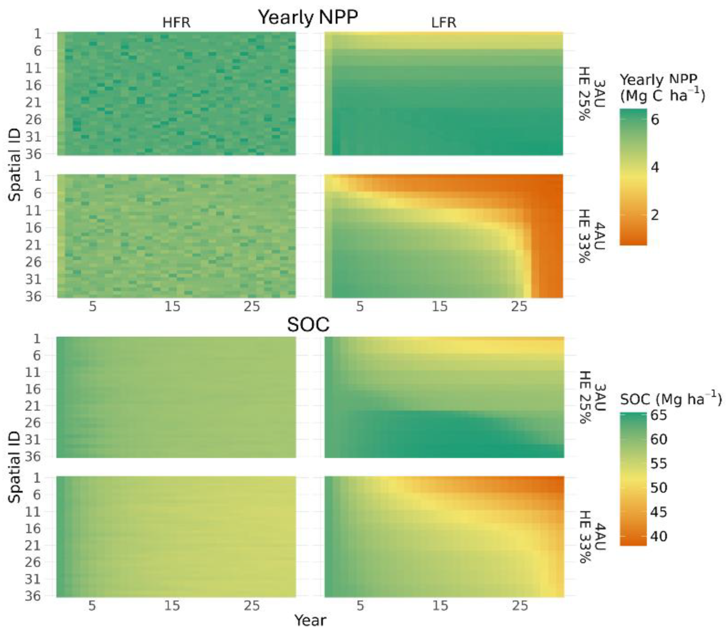
Figure 7.
Simulated soil organic carbon (SOC) stock in the 0 - 30 cm soil depth averaging over all spatial units, comparing the impacts of three weather scenarios (simulations with repeated one year of weather for annual precipitation representing average, wet, and dry conditions), seven stocking rate scenarios [2 to 5 AU ha-1 with corresponding harvest efficiency (HE)], two schedule patterns (2 and 3 events in a year), and two grazing management types [low frequency rotation (LFR) and high frequency rotation (HFR)].

3.3.2. Effect on SOC
Our simulation performed well at capturing the average baseline SOC stocks across plots for each soil depth (Figure S2), indicated by the low RMSE values of 6.87, 3.86, 3.07, and 7.89 Mg C ha-1 at 0-15, 15-30, 30-50, and 50-100 cm depth, respectively. These baseline SOC stocks were measured on soil samples collected in 2022, before the implementation of grazing treatments, and are therefore the cumulative result of prior, historical management. Future research will further evaluate the model’s accuracy in estimating the change in SOC stocks over time for the two treatments. Regardless, the model simulates the baseline conditions with relatively low error.
Regarding the simulated scenarios, the model predicted distinct SOC dynamics for the two management strategies in some of the simulated grazing scenarios. Under the average weather, similar to yearly NPP, the modeled average (averaged over all spatial units) topsoil SOC stocks (0 to 30 cm) remained relatively stable or showed a slight decline over time under light and moderate grazing intensities. Little or no differences were observed between HFR and LFR for either grazing schedule pattern at these intensities. However, as grazing intensity increased beyond moderate, SOC stocks began to decline more rapidly. Significant differences between HFR and LFR emerged at higher HE. At HE levels of 33% and 37% for two grazing events, and at 37% HE for three grazing events, the model predicted notable divergence in SOC stocks with greater SOC stocks in the HFR treatment. The largest difference in SOC was observed at the end of the 30-year simulation for the 37% HE scenario under two grazing events, where SOC stocks under LFR were 13.9 Mg C ha⁻¹ lower (a 26.9% reduction) compared to HFR. Furthermore, the model indicated a trend suggesting that this difference would continue to grow if the simulation were extended beyond 30 years. At highest grazing intensity (41% HE), the difference between the two management strategies diminished, with both HFR and LFR showing rapid SOC declines.
Under wet weather conditions, SOC dynamics followed a similar pattern to those under average weather conditions, with slightly higher SOC values after 30 years of simulation for these scenarios. In contrast, under dry weather conditions, the model predicted a slow decline in SOC over time even at light and moderate grazing intensities. Significant differences between HFR and LFR were observed at higher grazing intensities, including scenarios with 31%, 36%, and 41% HE under two grazing events, and 36%, 41%, and 46% HE under three grazing events. The largest difference was observed at the end of 30 years for the 36% HE scenario under two grazing events, where SOC stocks under LFR were 12.3 Mg C ha⁻¹ lower (a 22.7% reduction) compared to HFR. However, at the highest intensity (51% HE), predicted SOC stocks converged and declined rapidly, with no difference observed between management strategies. These patterns closely mirrored the NPP dynamics, although the divergence in SOC stocks appeared later in the simulation compared to NPP changes. In addition, trends in SOC for the subsoil (30 – 100 cm) were similar to the topsoil (Figure S4).
For the spatial patterns at the spatial unit level, a similar trend was observed for SOC as the yearly NPP in the two example scenarios under average weather conditions with two grazing events (Figure 6). Under LFR at moderate grazing intensity (25% HE), SOC in spatial units closer to the water source exhibited a slight decline, while spatial units farther from the water source maintained relatively stable SOC stocks. At higher grazing intensity (33% HE), where yearly NPP indicated system degradation, SOC declined rapidly across all spatial units, with greater declines in units closer to the water source. In contrast, under HFR, SOC remained uniform across spatial units, with only minor losses over time.
4. Discussion
4.1. The Field Experiment Data
The field experiment provided detailed information on grazing management, extensive measurements of plant and soil variables, and long-term historical management records. The inclusion of replicated plots for grazing management treatments further enhanced the dataset’s robustness, making it highly suitable for modeling plant-soil interactions. Using such a reliable dataset ensures that our model was tuned with real data and accurately represents real-world dynamics.
4.2. Plant Parameterization Performance
The MEMS 3.0 model predicted LAI and biomass with reasonable accuracy. Leaf area index is a crucial plant indicator because it estimates the amount of light intercepted by the plant canopy, which drives photosynthesis. It also influences water transpiration and soil evaporation, subsequently affecting soil moisture and all moisture-dependent processes, making it a critical variable for model calibration [66]. The ability to capture seasonal dynamics and grazing impacts suggests that the calibration effectively represented ecological processes driving plant canopy dynamics.
However, the model showed weaker performance in predicting aboveground biomass. This may be attributed to the fact that the model does not simulate the coexistence of multiple plant species. Instead, a single set of plant parameter values was used to represent a mixed community of grasses with diverse growth patterns. In monoculture systems, LAI and aboveground biomass are typically strongly correlated [66]. Our previous study on monoculture Bahia grass demonstrated the MEMS model’s strong predictive ability for aboveground biomass, achieving an R² of 0.72, which supports this explanation. In contrast, we observed a much weaker relationship in the mixed grass fields from our current study area (R2 of 0.20). The diversity of species, along with their varying leaf structures and biomass characteristics, likely contributed to the reduced correlation.
4.2. Comparison to the Grazing Distribution Pattern from Remote Sensing
Sentinel-2 provides high-resolution (10 m) data at a 5-day interval, making it highly suitable for analyzing spatial vegetation dynamics. However, cloud cover often limits the usability of these data, particularly in regions with frequent overcast conditions. Despite this challenge, our calculated ΔEVI effectively revealed differences between grazing and non-grazing periods. For example, the flat distribution of ΔEVI values observed before grazing in these plots indicated no significant spatial pattern. However, the wide spread of ΔEVI values in the spring of 2024 in the L3 plot was challenging to interpret. This variability may be attributed to the diverse plant species present at the site, including cool-season and warm-season grasses, which exhibit different growth dynamics during May.
The grazing effect was particularly evident in the L1 plot in 2022 (Figure 4), where the ΔEVI values demonstrated a clear spatial trend. The wider spread of ΔEVI values at similar distances to the water source compared to the non-grazing period suggested significant heterogeneity of the grazing distribution across the landscape. The two grazing periods in the L3 plot exhibited more variability in ΔEVI, likely influenced by additional factors affecting animal distribution, such as plant species composition and their productivity, proximity to fences, and the abundance of weeds. These spatial patterns align with the patchy structure commonly observed in grazing lands, which arises from the natural heterogeneity of soil and plant communities, coupled with the selective grazing behavior of animals [38]. However, it is important to note that the model does not account for all these influencing factors. As a result, the simulated ΔLAI trends lack the variability or “noise” when plotting them against distance to water source (Figure 4).
For the summer grazing in the L3 plot in 2023, the simulated ΔLAI exhibited a similar trend to ΔEVI but appeared more flattened. This was due to the modeled senescence of green leaves caused by drought conditions during the simulation. The spatial pattern of biomass intake by grazing animals during this period showed clear differences (Figure 4), indicating that the flattening of model predicted LAI was not solely a result of grazing but also influenced by environmental stressors. Additionally, in the L3 plot, a specific area located between 200 and 300 meters from the water source experienced heavier grazing than surrounding areas (low ΔEVI values in both years). This localized grazing pressure may be explained by differences in biomass production, the presence of more palatable grass species, or variations in soil properties that promote higher productivity. Interestingly, while the L3 plot exhibited a wider spatial spread of ΔEVI values compared to the L1 plot, the overall range of ΔEVI values remained comparable between the two plots. This observation suggests that while additional factors may influence the spatial distribution of grazing, they do not significantly alter the overall field-average effect. This finding supports the modeling simplification of incorporating only major factors, such as distance to water and forage availability, to capture the general trends in grazing distribution effectively.
4.3. The Modeling Scenarios
4.3.1. Response of Plant Productivity
Our results indicate that pasture systems can sustain productivity under light and moderate grazing intensities, with minimal differences between HFR and LFR. However, under heavy grazing intensities (HE between30% and 40%), HFR demonstrated a greater ability to maintain productivity, whereas LFR exhibited signs of degradation. At very high grazing intensities (above 40% HE), the system showed signs of fast degradation, regardless of grazing rotation frequency or the scheduled patterns of grazing.
These findings are supported by field studies that highlight the advantages of HFR under higher grazing intensities. For example, Heitschmidt et al. [69] observed sustainable production with an average HE of 42% over four years on a mixed native grass ranch in Texas using HFR. Similarly, Teague et al. [12] found that HFR resulted in significantly higher plant cover compared to continuous grazing under heavy grazing intensities. Wang et al. [70] reported higher forage production in an HFR-managed ranch compared to an LFR-managed ranch in Mississippi. Norton [71], after analyzing multiple grazing trials, also concluded that HFR can offer substantial benefits for sustaining productivity under heavy grazing pressure.
However, not all studies have found HFR to be superior to LFR or continuous grazing. Teague et al. [38] suggested that differences in spatial and temporal scales, as well as variations in management practices across experiments, could explain the inconsistent findings. This hypothesis aligns well with our modeling results. First, our simulations suggest that the differences between HFR and LFR (and potentially continuous grazing) only become apparent under specific grazing intensities, particularly heavy grazing. Second, significant responses to grazing management may take years to measurably impact the system, possibly due to the high natural heterogeneity of grazing lands. Third, the size of grazing plots plays an important role. The plots in our study were sufficiently large to observe non-uniform grazing distribution patterns, whereas smaller plots, as used in some other experiments [38], may not allow grazing distribution to differ substantially between HFR and LFR systems.
In terms of weather conditions, our simulations showed minimal differences in productivity between wet and average weather scenarios. In the wet weather simulation, above-average rainfall occurred primarily in May and June, followed by a dry summer, while rainfall in the average weather scenario was more evenly distributed throughout the year. Despite higher annual precipitation in the wet weather scenario, total production remained similar across both scenarios. However, the timing of water stress differed in these scenarios. Under average weather, significant water stress was simulated in August, whereas in the wet weather scenario, water stress was concentrated in September and October. This suggests that the timing of precipitation and subsequent water stress plays a critical role in determining productivity, even when total annual rainfall is higher.
Our simulations also highlighted the interaction between grazing schedule patterns, stocking rate, rotation frequency, timing, and duration. For both HFR and LFR systems, production under two grazing events declined at lower stocking rates, which may be attributed to the longer grazing duration of each event. Extended grazing periods resulted in greater biomass removal, slowed recovery rates, and triggered a cascade effect that hindered grass growth in subsequent periods. Since grazing management schedules can be highly complex, our simulations emphasize the importance of considering these interactions when designing grazing experiments, as they can significantly impact productivity outcomes.
One key finding of our study is that uneven grazing distribution underlies the differences between HFR and LFR. Our model focused on general trends in grazing distribution, highlighting how uneven pressure under LFR impacts plant productivity. Similarly, Wang et al. [72] used an empirical plant growth model to simulate uneven grazing distribution caused by selective grazing. Their model incorporated two types of grasses—palatable and less-palatable—and accounted for differential defoliation rates. At the commercial ranching scale, their simulations showed that HFR grazing excels across a wide range of scenarios in terms of grass productivity, particularly under high stocking rates. These findings align with our results, which demonstrate that uneven grazing pressure under LFR and continuous grazing leads to reduced productivity compared to HFR, the effect of which becomes more pronounced at certain range of higher grazing intensities. However, it is important to note that their study was primarily a theoretical exploration and lacked spatially explicit representation of real-world field conditions. Nonetheless, both studies underscore the importance of addressing uneven grazing pressure when comparing grazing strategies.
The gradual changes in spatial distribution of plant productivity over time (Figure 6) observed in our study further highlight the dynamic nature of grazing systems. These changes suggest that the effects of uneven grazing distribution cannot be captured by a single 1D simulation or multiple disconnected 1D simulations with prescribed grazing intensities. Grazing distribution is highly dynamic at both daily and long-term scales, as demonstrated in our simulations. This underscores the need for spatially explicit modeling approaches, as the one we demonstrated here using MEMS 3.0, which accounts for the evolving interactions between grazing pressure, plant productivity, and SOC dynamics over time.
4.3.2. Response of SOC and Implications for Experimental Design
Overall, our simulated SOC changes over time align well with findings from field studies. Light and moderate grazing intensities were shown to sustain SOC levels, while heavy grazing generally led to system degradation reflected by significant SOC loss—patterns that have been well-documented in previous studies [2,12,73,74]. However, since we only have a single time-point measurement of SOC, it was not possible to directly evaluate the simulated long-term trends. This highlights the need for additional field data collected over extended periods to verify the model’s predictions and improve its reliability.
Our simulations further highlight the critical role of grazing distribution in shaping SOC dynamics. Under LFR management, uneven animal distribution concentrates grazing pressure in preferred areas, particularly those closer to water sources. As grazing intensity increases, these heavily grazed areas experience declining plant productivity, which subsequently leads to significant SOC loss. The loss of SOC indicates a depletion of organic matter and essential nutrients, which initiates a positive feedback loop where reduced plant productivity further exacerbates SOC depletion (Figure 6). Over time, these overgrazed areas expand and become more contiguous across the pasture, leading to widespread degradation of the system. In contrast, HFR promotes more uniform grazing distribution, preventing localized overgrazing and enabling the system to sustain higher overall grazing intensities before tipping into long-term decline. This finding aligns closely with the hypothesis proposed by Teague et al. [38].
Our findings support a hypothesis that HFR can increase SOC by applying high stocking density for short duration, with frequent animal movement among paddocks that promotes more uniform grazing across the pasture. Experiments are needed to further evaluate these modelling results. Some field studies suggest that HFR grazing management can support greater SOC storage than LFR grazing [8,9,11,12], but there are other studies that report no significant effects [75,76]. As noted by Teague et al. [38], inconsistencies in the results of existing studies may stem from differences in spatial and temporal scales, as well as interactions with regulating factors such as climate, soil properties, and vegetation composition. Specifically, as discussed earlier, plot size must be sufficiently large to enable the development of uneven grazing distribution, which is a key factor driving differences between grazing management strategies. Small plots may fail to capture the spatial heterogeneity of grazing pressure, limiting the ability to observe differences between treatments. Long-term monitoring (>10 years) is also essential to capture slow processes influencing SOC dynamics, which require extended time frames to observe significant changes [77]. Additionally, our results suggest that experimental designs should include high grazing intensities to better understand the thresholds at which ecosystem degradation occurs and to identify differences between grazing strategies, such as HFR and LFR, under stress conditions.
4.4. Model Limitations and Future Improvements
There are certain limitations in the dataset used for this study. Firstly, grazing intensity was managed within a moderate range and was not included as a treatment variable, limiting the ability to assess its effects across a wider range of intensities. Another limitation of the dataset is the current lack of longitudinal SOC measurements, which are essential for evaluating the model’s predictions on SOC changes over time. However, the dataset does include two years of eddy covariance tower measurements from the study site, which were used to evaluate short-term net ecosystem exchange (NEE) of C under these treatments using this version of MEMS model, as reported in Santos et al. [51], with quantified model uncertainty. Furthermore, the model was evaluated for short-term NEE using data from three additional grazing experiments within the 3M project, as described in Santos et al. [51].
While our model successfully simulated general grazing distribution influenced by major factors, such as distance to water, it was limited by simplifications in the model simulation framework. These simplifications did not address all factors that significantly influence animal distribution, including heterogeneity in plant composition, social behaviors, and localized environmental characteristics. These factors likely contributed to the observed spatial variability in grazing patterns and plant responses, highlighting the necessity of incorporating more of the inherent complexity of grazing systems in future modeling studies.
One particularly challenging aspect is the selective grazing behavior of ruminants, which creates patchiness in the landscape and localized grazing distribution as they preferentially consume more palatable species. Capturing this fine-scale heterogeneity in process-based models remains difficult, primarily due to the lack of high-resolution soil and vegetation data required as inputs. Acquiring such detailed measurements is often costly and logistically challenging, yet this level of input would significantly enhance the accuracy of the simulated distribution of grazing across a field. Although incorporating these additional factors and datasets would enhance the spatial accuracy of grazing distribution predictions, it is important to note that such improvements may yield limited benefits when focusing solely on field-average forage production and SOC dynamics. The general trends and ranges of the effect are captured at the scale of the entire field by the main factors such as forage amount/quality and distance to drinking water according to our study.
One of the primary limitations of our MEMS 3.0 model is its representation of the plant community as a single species. Model parameters were fitted to reflect the overall growth of the plant community rather than the dynamics of individual species. While this simplification is common in ecosystem modeling (e.g., PaSim, DayCent, and APSIM) and often provides generally acceptable results, it reduces the accuracy of predictions for overall biomass and LAI. There have been attempts to simulate species composition and competition on grazing lands in other studies: for example, the SPUR rangeland model simulated multiple species [78] but was not accurate in predicting the dynamics leading to variation in species composition. Regardless, this simplification limits MEMS ability to fully capture the complex interactions between grazing management and plant growth processes in ecosystems with high plant diversity. Future improvements to the model could focus on simulating simplified plant communities composed of functional groups, such as C3 and C4 grasses or legume (generally palatable and fix nitrogen) and non-legume plants.
Another limitation of the model is its inability to simulate lateral processes, such as surface water runoff and associated soil erosion. These processes can play a significant role in shaping grazing lands, particularly in areas with steep slopes or uneven terrain. As our spatially explicit implementation does not currently account for lateral flows between spatial units, the model is not suitable for fields where lateral water movement is a dominant factor. Future model development will aim to address these processes, potentially by adapting lateral water routing methods from established models such as the APEX model [79].
5. Conclusions
This study demonstrates the utility of process-based ecosystem modeling for understanding the interactions between grazing management, plant dynamics, and SOC storage. We incorporated spatially explicit grazing distribution into the MEMS ecosystem model and used distance to water as the primary factor influencing grazing patterns in the experimental fields. The simulated grazing distribution closely aligned with general patterns observed in satellite imagery, supporting the model’s ability to capture realistic grazing dynamics.
Using the new MEMS model, we found that light and moderate grazing intensities generally sustain forage production and SOC, while very high grazing intensity could lead to rapid degradation at this site. High-frequency rotation mitigates localized overgrazing and supports higher grazing intensities compared to LFR, although degradation occurs at very high intensities under both strategies. Uneven grazing distribution was identified as a critical factor driving reduced productivity and SOC loss under LFR, underscoring the role of spatial heterogeneity in shaping grazing system outcomes.
These results underscore the limitations of existing process-based models, which often assume uniform grazing and fail to incorporate the nuanced effects of selective grazing behavior and landscape heterogeneity. While such models have been used for large-scale simulations to inform grazing management decisions, our findings suggest their predictions may be biased without accounting for spatial grazing dynamics. Field research is urgently needed to evaluate these predictions and ensure that models are reliable tools for regional and global carbon management.
Data and Software Availability
The MEMS 3.0 model’s license will be available from the Soil Carbon Solution Center (https://www.soilcarbonsolutionscenter.com) at Colorado State University; free for academic collaborations. The experimental measurement data is available on request. Sentinel-2 Level-2A data were accessed through the Earth Search STAC API hosted by Element 84 (https://earth-search.aws.element84.com/v1). This dataset consists of Cloud-Optimized GeoTIFFs (COGs) derived from the original Copernicus Sentinel-2 archives.
CRediT Authorship Contribution Statement
Yao Zhang: Writing – review & editing, Writing – original draft, Software, Methodology, Investigation, Formal analysis, Data curation, Conceptualization, Funding acquisition. Rafael S. Santos: Writing – review & editing, Writing – original draft, Methodology, Investigation, Formal analysis, Data curation, Conceptualization. Emma K. Hamilton: Writing – review & editing, Writing – original draft, Software, Methodology, Investigation, Formal analysis, Data curation, Conceptualization. Paige L. Stanley: Writing – review & editing, Data curation, Methodology. Hao Yang: Writing – review & editing, Data curation, Methodology. Keith Paustian: Writing – review & editing, Methodology. Erica L. Patterson: Writing – review & editing. Stephen M. Ogle Writing – review & editing, Methodology. Isabella C. F. Maciel: Writing – review & editing, Data curation, Methodology. Guilhermo F. S. Congio: Writing – review & editing. Hugh Aljoe: Writing – review & editing. Alejandro Romero-Ruiz: Methodology, Writing – review & editing. Jeff J. Goodwin: Writing – review & editing. Jason Rowntree: review & editing, Funding acquisition. M. Francesca Cotrufo: Writing – review & editing, Writing – original draft, Methodology, Funding acquisition, Conceptualization.
Declaration of Competing Interest
Yao Zhang, Rafael S. Santos, Emma K. Hamilton, Keith Paustian, and M. Francesca Cotrufo receive a portion of the licensing fees associated with the MEMS model. M. Francesca Cotrufo discloses to be a cofounder and Science Director of Cquester Analytics LLC. All other authors declare no known competing financial interests or personal relationships that could have influenced the work reported in this paper.
Declaration of Generative AI and AI-Assisted Technologies in the Writing Process
During the preparation of this work the authors used ChatGPT and Google Gemini in order to improve readability and language. After using these tools, the authors reviewed and edited the content as needed and take full responsibility for the content of the publication.
Supplementary Materials
The following supporting information can be downloaded at the website of this paper posted on Preprints.org.
Acknowledgments
This research was supported by a project funded by the Foundation for Food and Agriculture Research (FFAR grant number: DSnew-0000000028), The Noble Research Institute, Greenacres Foundation, and Butcherbox. It was also supported by the United States Department of Agriculture (USDA agreement number NR233A750004G050), and Shell International Exploration and Production Inc. (contract n. CW517568). The content of this publication is solely the responsibility of the authors and does not necessarily represent the official views of our funders. The authors also thank Dr. Feng Gao, Dr. Justin Derner, and Dr. Martha Anderson for providing ground measurement protocols and Dr. Sean P. Kearney and Dr. Erika S. Peirce for data discussions. We also thank Dr. Randall Boone, and Yezzen Khazindar from Colorado State University for relevant discussions regarding grazing management and data analysis. The Sentinel-2 data were downloaded using the Earth Search STAC API hosted by Element 84, which contains modified Copernicus Sentinel data processed by Element 84.
References
- FAO. Land statistics 2001–2022. Global, regional and country trends [Internet]; FAO: Rome, Italy; Available online: https://openknowledge.fao.org/handle/20.500.14283/cd1484en.
- Bai, Y; Cotrufo, MF. Grassland soil carbon sequestration: Current understanding, challenges, and solutions. Science 2022, 377(6606), 603–608. [Google Scholar] [CrossRef] [PubMed]
- McSherry, ME; Ritchie, ME. Effects of grazing on grassland soil carbon: a global review. Global Change Biology 2013, 19(5), 1347–1357. [Google Scholar] [CrossRef]
- Ren, S; Terrer, C; Li, J; Cao, Y; Yang, S; Liu, D. Historical impacts of grazing on carbon stocks and climate mitigation opportunities. Nature Climate Change 2024, 14(4), 380–386. [Google Scholar] [CrossRef]
- Sanderman, J; Hengl, T; Fiske, GJ. Soil carbon debt of 12,000 years of human land use. PNAS 2017, 114(36), 9575–9580. [Google Scholar] [CrossRef]
- Paustian, K; Lehmann, J; Ogle, S; Reay, D; Robertson, GP; Smith, P. Climate-smart soils. Nature 2016, 532(7597), 49–57. [Google Scholar] [CrossRef]
- Stanley, PL; Wilson, C; Patterson, E; Machmuller, MB; Cotrufo, MF. Ruminating on soil carbon: Applying current understanding to inform grazing management. Global Change Biology 2024, 30(3), e17223. [Google Scholar] [CrossRef]
- Mehre, J; Schneider, K; Jayasundara, S; Gillespie, A; Wagner-Riddle, C. Adaptive multi-paddock grazing increases soil carbon stocks and decreases the carbon footprint of beef production in Ontario, Canada. Journal of Environmental Management 2024, 371, 123255. [Google Scholar] [CrossRef] [PubMed]
- Mosier, S; Apfelbaum, S; Byck, P; et al. Adaptive multi-paddock grazing enhances soil carbon and nitrogen stocks and stabilization through mineral association in southeastern U.S. grazing lands. Journal of Environmental Management 2021, 288, 112409. [Google Scholar] [CrossRef]
- Santos, RS; Hamilton, EK; Stanley, PL; Paustian, K; Cotrufo, MF; Zhang, Y. Simulating adaptive grazing management on soil organic carbon in the Southeast U.S.A. using MEMS 2. Journal of Environmental Management 2024, 365, 121657. [Google Scholar] [CrossRef] [PubMed]
- Stanley, PL; Rowntree, JE; Beede, DK; DeLonge, MS; Hamm, MW. Impacts of soil carbon sequestration on life cycle greenhouse gas emissions in Midwestern USA beef finishing systems. Agricultural Systems 2018, 162, 249–258. [Google Scholar] [CrossRef]
- Teague, WR; Dowhower, SL; Baker, SA; Haile, N; DeLaune, PB; Conover, DM. Grazing management impacts on vegetation, soil biota and soil chemical, physical and hydrological properties in tall grass prairie. Agriculture, Ecosystems & Environment 2011, 141(3), 310–322. [Google Scholar] [CrossRef]
- Stanley, P; Roche, L; Bowles, T. Amping up soil carbon: soil carbon stocks in California rangelands under adaptive multi-paddock and conventional grazing management. International Journal of Agricultural Sustainability 2025, 23(1), 2461826. [Google Scholar] [CrossRef]
- Augustine, DJ; Kearney, SP; Raynor, EJ; Porensky, LM; Derner, JD. Adaptive, multi-paddock, rotational grazing management alters foraging behavior and spatial grazing distribution of free-ranging cattle. Agriculture, Ecosystems & Environment 2023, 352, 108521. [Google Scholar]
- Barnes, MK; Norton, BE; Maeno, M; Malechek, JC. Paddock Size and Stocking Density Affect Spatial Heterogeneity of Grazing. Rangeland Ecology & Management 2008, 61(4), 380–388. [Google Scholar] [CrossRef]
- Romero-Ruiz, A; Rivero, MJ; Milne, A; et al. Grazing livestock move by Lévy walks: Implications for soil health and environment. Journal of Environmental Management 2023, 345, 118835. [Google Scholar] [CrossRef]
- Brock, BL; Owensby, CE. Predictive Models for Grazing Distribution: A GIS Approach. Journal of Range Management 2000, 53(1), 39–46. [Google Scholar] [CrossRef]
- Bailey, Derek W.; Gross, JE; Laca, EA; et al. Mechanisms That Result in Large Herbivore Grazing Distribution Patterns. Journal of Range Management 1996, 49(5), 386–400. [Google Scholar] [CrossRef]
- Pringle, HJR; Landsberg, J. Predicting the distribution of livestock grazing pressure in rangelands. Austral Ecology 2004, 29(1), 31–39. [Google Scholar] [CrossRef]
- Goulart, RCD; Corsi, M; Bailey, DW; Zocchi, SS. Cattle Grazing Distribution and Efficacy of Strategic Mineral Mix Placement in Tropical Brazilian Pastures. Rangeland Ecology & Management 2008, 61(6), 656–660. [Google Scholar] [CrossRef]
- Thrash, I; Derry, JF. The nature and modelling of piospheres: a review. Koedoe 1999, 42(2), 73–94. [Google Scholar] [CrossRef]
- Dumont, B; Hill, DRC. Spatially explicit models of group foraging by herbivores: what can Agent-Based Models offer? Anim. Res. 2004, 53(5), 419–428. [Google Scholar] [CrossRef]
- Guerrin, F. Agent-Based Modelling of a Simple Synthetic Rangeland Ecosystem [Internet]. In Landscape Modelling and Decision Support; Available from; Mirschel, W, Terleev, VV, Wenkel, K-O, Eds.; Springer International Publishing: Cham, 2020; pp. 179–215. [Google Scholar] [CrossRef]
- Yoshihara, Y; Horie, R; Miyasaka, T; Kono, A; Shinoda, M. Predicting livestock intake energy at different grazing strategies using agent-based modelling of livestock. Sci Rep. 2025, 15(1), 35906. [Google Scholar] [CrossRef]
- Coughenour, MB. Spatial Modeling and Landscape Characterization of an African Pastoral Ecosystem: A Prototype Model and its Potential Use for Monitoring Drought [Internet]. In Ecological Indicators; Available from; McKenzie, DH, Hyatt, DE, McDonald, VJ, Eds.; Springer US: Boston, MA, 1992; Volume 1, pp. 787–810. [Google Scholar] [CrossRef]
- Marohn, C; Troost, C; Warth, B; et al. Coupled biophysical and decision-making processes in grassland systems in East African savannahs – A modelling framework. Ecological Modelling 2022, 474, 110113. [Google Scholar] [CrossRef]
- Teague, R; Kreuter, U. Managing Grazing to Restore Soil Health, Ecosystem Function, and Ecosystem Services. Front. Sustain. Food Syst. [Internet] 2020, 4. Available online: https://www.frontiersin.org/journals/sustainable-food-systems/articles/10.3389/fsufs.2020.534187/full. [CrossRef]
- Sándor, R; Picon-Cochard, C; Martin, R; et al. Plant acclimation to temperature: Developments in the Pasture Simulation model. Field Crops Research 2018, 222, 238–255. [Google Scholar] [CrossRef]
- Vuichard, N; Soussana, J-F; Ciais, P; et al. Estimating the greenhouse gas fluxes of European grasslands with a process-based model: 1. Model evaluation from in situ measurements. Global Biogeochemical Cycles [Internet] 2007, 21(1). Available online: https://onlinelibrary.wiley.com/doi/abs/10.1029/2005GB002611. [CrossRef]
- Parton, WJ; Hartman, M; Ojima, D; Schimel, D. DAYCENT and its land surface submodel: description and testing. Global and Planetary Change 1998, 19(1), 35–48. [Google Scholar] [CrossRef]
- Shepherd, A; Hartman, MD; Fitton, N; et al. Metrics of biomass, live-weight gain and nitrogen loss of ryegrass sheep pasture in the 21st century. Science of The Total Environment 2019, 685, 428–441. [Google Scholar] [CrossRef]
- Chang, X; Bao, X; Wang, S; et al. Simulating effects of grazing on soil organic carbon stocks in Mongolian grasslands. Agriculture, Ecosystems & Environment 2015, 212, 278–284. [Google Scholar] [CrossRef]
- Parton, WJ; Stewart, JWB; Cole, CV. Dynamics of C, N, P and S in grassland soils: a model. Biogeochemistry 1988, 5(1), 109–131. [Google Scholar] [CrossRef]
- Li, C; Frolking, S; Frolking, TA. A model of nitrous oxide evolution from soil driven by rainfall events: 1. Model structure and sensitivity. Journal of Geophysical Research: Atmospheres 1992, 97(D9), 9759–9776. [Google Scholar] [CrossRef]
- Zhang, W; Zhang, F; Qi, J; Hou, F. Modeling impacts of climate change and grazing effects on plant biomass and soil organic carbon in the Qinghai–Tibetan grasslands. Biogeosciences 2017, 14(23), 5455–5470. [Google Scholar] [CrossRef]
- O’Leary, GJ; Liu, DL; Ma, Y; et al. Modelling soil organic carbon 1. Performance of APSIM crop and pasture modules against long-term experimental data. Geoderma 2016, 264, 227–237. [Google Scholar] [CrossRef]
- Wang, J; Li, Y; Bork, EW; et al. Modelling spatio-temporal patterns of soil carbon and greenhouse gas emissions in grazing lands: Current status and prospects. Science of The Total Environment 2020, 739, 139092. [Google Scholar] [CrossRef]
- Teague, R; Provenza, F; Kreuter, U; Steffens, T; Barnes, M. Multi-paddock grazing on rangelands: Why the perceptual dichotomy between research results and rancher experience? Journal of Environmental Management 2013, 128, 699–717. [Google Scholar] [CrossRef]
- Zhang, Y; Lavallee, JM; Robertson, AD; et al. Simulating measurable ecosystem carbon and nitrogen dynamics with the mechanistically defined MEMS 2.0 model. Biogeosciences 2021, 18(10), 3147–3171. [Google Scholar] [CrossRef]
- Boone, RB; Coughenour, MB; Galvin, KA; Ellis, JE. Addressing management questions for Ngorongoro Conservation Area, Tanzania, using the Savanna modelling system. African Journal of Ecology 2002, 40(2), 138–150. [Google Scholar] [CrossRef]
- Bunting, EL; Fullman, T; Kiker, G; Southworth, J. Utilization of the SAVANNA model to analyze future patterns of vegetation cover in Kruger National Park under changing climate. Ecological Modelling 2016, 342, 147–160. [Google Scholar] [CrossRef]
- Christensen, L; Coughenour, MB; Ellis, JE; Chen, Z. Sustainability of Inner Mongolian Grasslands: Application of the Savanna Model. Journal of Range Management 2003, 56(4), 319–327. [Google Scholar] [CrossRef]
- Cotrufo, MF; Soong, JL; Horton, AJ; et al. Formation of soil organic matter via biochemical and physical pathways of litter mass loss. Nature Geoscience 2015, 8(10), 776–779. [Google Scholar] [CrossRef]
- Liang, C; Schimel, JP; Jastrow, JD. The importance of anabolism in microbial control over soil carbon storage. Nature Microbiology 2017, 2(8), 17105. [Google Scholar] [CrossRef]
- Sokol, NW; Sanderman, J; Bradford, MA. Pathways of mineral-associated soil organic matter formation: Integrating the role of plant carbon source, chemistry, and point of entry. Global Change Biology 2019, 25(1), 12–24. [Google Scholar] [CrossRef] [PubMed]
- Allen, V g.; Batello, C; Berretta, E j.; et al. An international terminology for grazing lands and grazing animals. Grass and Forage Science 2011, 66(1), 2–28. [Google Scholar] [CrossRef]
- Guthery, FS; Bingham, RL. A Theoretical Basis for Study and Management of Trampling by Cattle. Journal of Range Management 1996, 49(3), 264. [Google Scholar] [CrossRef]
- Celia, MA; Bouloutas, ET; Zarba, RL. A general mass-conservative numerical solution for the unsaturated flow equation. Water Resources Research 1990, 26(7), 1483–1496. [Google Scholar] [CrossRef]
- Zha, Y; Yang, J; Yin, L; Zhang, Y; Zeng, W; Shi, L. A modified Picard iteration scheme for overcoming numerical difficulties of simulating infiltration into dry soil. Journal of Hydrology 2017, 551, 56–69. [Google Scholar] [CrossRef]
- Bittelli, M; Campbell, GS; Tomei, F. Soil physics with Python: transport in the soil-plant-atmosphere system; Oxford University Press: Oxford.
- Santos, RS; Hamilton, EK; Stanley, PL; et al. Applying the MEMS 3.0 model across contrasting grazing US ecoregions and managements: model uncertainty and evaluation. Under preparation.
- Stanley, PL; Kuhl, AS; Rowntree, JE; et al. Merging Rigor and Relevance in Grazingland Research: A Comprehensive Social-Ecological Monitoring Approach. Under review.
- European Space Agency. Sentinel-2 Level-2A MSI: MultiSpectral Instrument, Surface Reflectance [Data set]. Accessed via Earth Search STAC API (Element 84). sentinel-2-l2a collection. Available online: https://earth-search.aws.element84.com/v1/collections/sentinel-2-l2a (accessed on 2025).
- Huete, A; Didan, K; Miura, T; Rodriguez, EP; Gao, X; Ferreira, LG. Overview of the radiometric and biophysical performance of the MODIS vegetation indices. Remote Sensing of Environment 2002, 83(1), 195–213. [Google Scholar] [CrossRef]
- R Core Team. R: A Language and Environment for Statistical Computing [Internet]. 2025. Available online: https://www.R-project.org/.
- Abatzoglou, JT. Development of gridded surface meteorological data for ecological applications and modelling. International Journal of Climatology 2013, 33(1), 121–131. [Google Scholar] [CrossRef]
- Beaudette, D; Skovlin, J; Roecker, S; Brown, A. soilDB: Soil Database Interface [Internet]. 2025. Available online: https://cran.r-project.org/web/packages/soilDB/index.html.
- Schaap, MG; Leij, FJ; van Genuchten, MTh. rosetta: a computer program for estimating soil hydraulic parameters with hierarchical pedotransfer functions. Journal of Hydrology 2001, 251(3), 163–176. [Google Scholar] [CrossRef]
- Pebesma, E; Bivand, R. Spatial Data Science: With Applications in R [Internet], 1st ed.; Chapman and Hall/CRC: New York; Available online: https://www.taylorfrancis.com/books/9780429459016.
- Knapp, AK; Blair, JM; Briggs, JM; et al. The Keystone Role of Bison in North American Tallgrass Prairie: Bison increase habitat heterogeneity and alter a broad array of plant, community, and ecosystem processes. BioScience 1999, 49(1), 39–50. [Google Scholar] [CrossRef]
- Guyette, RP; Stambaugh, MC; Dey, DC; Muzika, R-M. Predicting Fire Frequency with Chemistry and Climate. Ecosystems 2012, 15(2), 322–335. [Google Scholar] [CrossRef]
- Sloat, LL; Gerber, JS; Samberg, LH; et al. Increasing importance of precipitation variability on global livestock grazing lands. Nature Clim Change 2018, 8(3), 214–218. [Google Scholar] [CrossRef]
- Bidwell, T; Elmore, D; Hickman, K. Stocking Rate Determination on Native Rangeland [Internet]; Oklahoma State University Extension, 2017; Available online: https://extension.okstate.edu/fact-sheets/stocking-rate-determination-on-native-rangeland.html.
- Smart, AJ; Derner, JD; Hendrickson, JR; et al. Effects of Grazing Pressure on Efficiency of Grazing on North American Great Plains Rangelands. Rangeland Ecology & Management 2010, 63(4), 397–406. [Google Scholar] [CrossRef]
- Hamner, B; Frasco, M; LeDell, E. Metrics: Evaluation Metrics for Machine Learning [Internet]. 2018. Available online: https://cran.r-project.org/web/packages/Metrics/index.html.
- Zhang, Y; Suyker, A; Paustian, K. Improved Crop Canopy and Water Balance Dynamics for Agroecosystem Modeling Using DayCent. Agronomy Journal. 2018, 110(2), 511–524. [Google Scholar] [CrossRef]
- Kang, Y; Özdoğan, M; Zipper, SC; et al. How Universal Is the Relationship between Remotely Sensed Vegetation Indices and Crop Leaf Area Index? A Global Assessment. Remote Sensing [Internet]. 2016, 8. Available online: https://www.mdpi.com/2072-4292/8/7/597.
- Wang, J; Xiao, X; Bajgain, R; et al. Estimating leaf area index and aboveground biomass of grazing pastures using Sentinel-1, Sentinel-2 and Landsat images. ISPRS Journal of Photogrammetry and Remote Sensing 2019, 154, 189–201. [Google Scholar] [CrossRef]
- Heitschmidt, R; Dowhower, S; Walker, J. 14- vs. 42-paddock rotational grazing: aboveground biomass dynamics, forage production, and harvest efficiency. Journal of Range Management 1987, 40(3), 216–223. [Google Scholar] [CrossRef]
- Wang, F; Apfelbaum, SI; Thompson, RL; Teague, R; Byck, P. Effects of adaptive multiple paddock and continuous grazing on fine-scale spatial patterns of vegetation species and biomass in commercial ranches. Landscape Ecol. 2021, 36(9), 2725–2741. [Google Scholar] [CrossRef]
- Norton, B. The application of grazing management to increase sustainable livestock production. Animal production in Australia 1998, 22(1), 15–26. [Google Scholar]
- Wang, T; Teague, WR; Park, SC. Evaluation of Continuous and Multipaddock Grazing on Vegetation and Livestock Performance—a Modeling Approach. Rangeland Ecology & Management 2016, 69(6), 457–464. [Google Scholar] [CrossRef]
- Milchunas, DG; Lauenroth, WK. Quantitative Effects of Grazing on Vegetation and Soils Over a Global Range of Environments. Ecological Monographs 1993, 63(4), 327–366. [Google Scholar] [CrossRef]
- Zhou, G; Zhou, X; He, Y; et al. Grazing intensity significantly affects belowground carbon and nitrogen cycling in grassland ecosystems: a meta-analysis. Global Change Biology 2017, 23(3), 1167–1179. [Google Scholar] [CrossRef]
- Hillenbrand, M; Thompson, R; Wang, F; Apfelbaum, S; Teague, R. Impacts of holistic planned grazing with bison compared to continuous grazing with cattle in South Dakota shortgrass prairie. Agriculture, Ecosystems & Environment 2019, 279, 156–168. [Google Scholar] [CrossRef]
- Shrestha, BM; Bork, EW; Chang, SX; et al. Adaptive Multi-Paddock Grazing Lowers Soil Greenhouse Gas Emission Potential by Altering Extracellular Enzyme Activity. Agronomy 2020, 10(11), 1781. [Google Scholar] [CrossRef]
- Oduor, CO; Karanja, NK; Onwonga, RN; Mureithi, SM; Pelster, D; Nyberg, G. Enhancing soil organic carbon, particulate organic carbon and microbial biomass in semi-arid rangeland using pasture enclosures. BMC Ecol. 2018, 18(1), 45. [Google Scholar] [CrossRef]
- Corson, MS; Skinner, RH; Rotz, CA. Modification of the SPUR rangeland model to simulate species composition and pasture productivity in humid temperate regions. Agricultural Systems 2006, 87(2), 169–191. [Google Scholar] [CrossRef]
- Williams, JR; Arnold, JG; Srinivasan, R; Ramanarayanan, TS. APEX: A New Tool for Predicting the Effects of Climate and CO2 Changes on Erosion and Water Quality. In Modelling Soil Erosion by Water; Boardman, J, Favis-Mortlock, D, Eds.; Springer Berlin Heidelberg, 1998; pp. 441–449. [Google Scholar]
Figure 1.
Schematic representation of livestock distribution under (a) low frequency rotation (LFR; a single large field under LFR with uneven livestock distribution driven by proximity to water) and (b) high frequency rotation (HFR; partitioning the pasture into a series of small paddocks and systematically rotating the herd through them) grazing management. The gray grid represents the spatial units used in the model, with numerical IDs assigned to each unit. Smaller ID numbers correspond to units located closer to the water source. The background images of pastures were generated by Google Gemini AI.
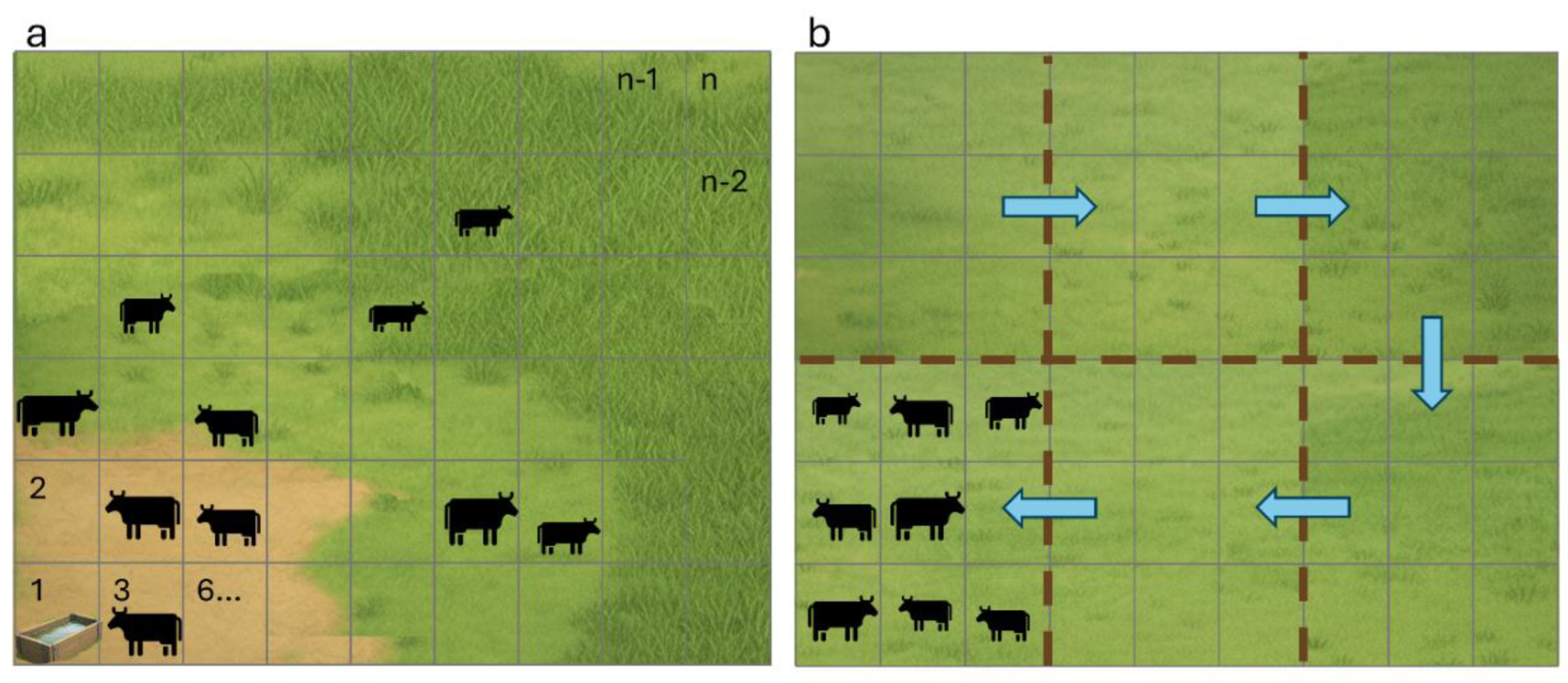
Figure 2.
Measured (dots) and simulated (lines) leaf area index (LAI) for each treatment plot managed under high frequency rotation (HFR; replicate plots H1-H3) and low frequency rotation (LFR; replicate plots L1-L3) grazing, at the Coffey Ranch in south-central Oklahoma, USA. Gray shading indicates grazing events. Vertical bars represent the standard deviation of the mean for measured values (n = 9).
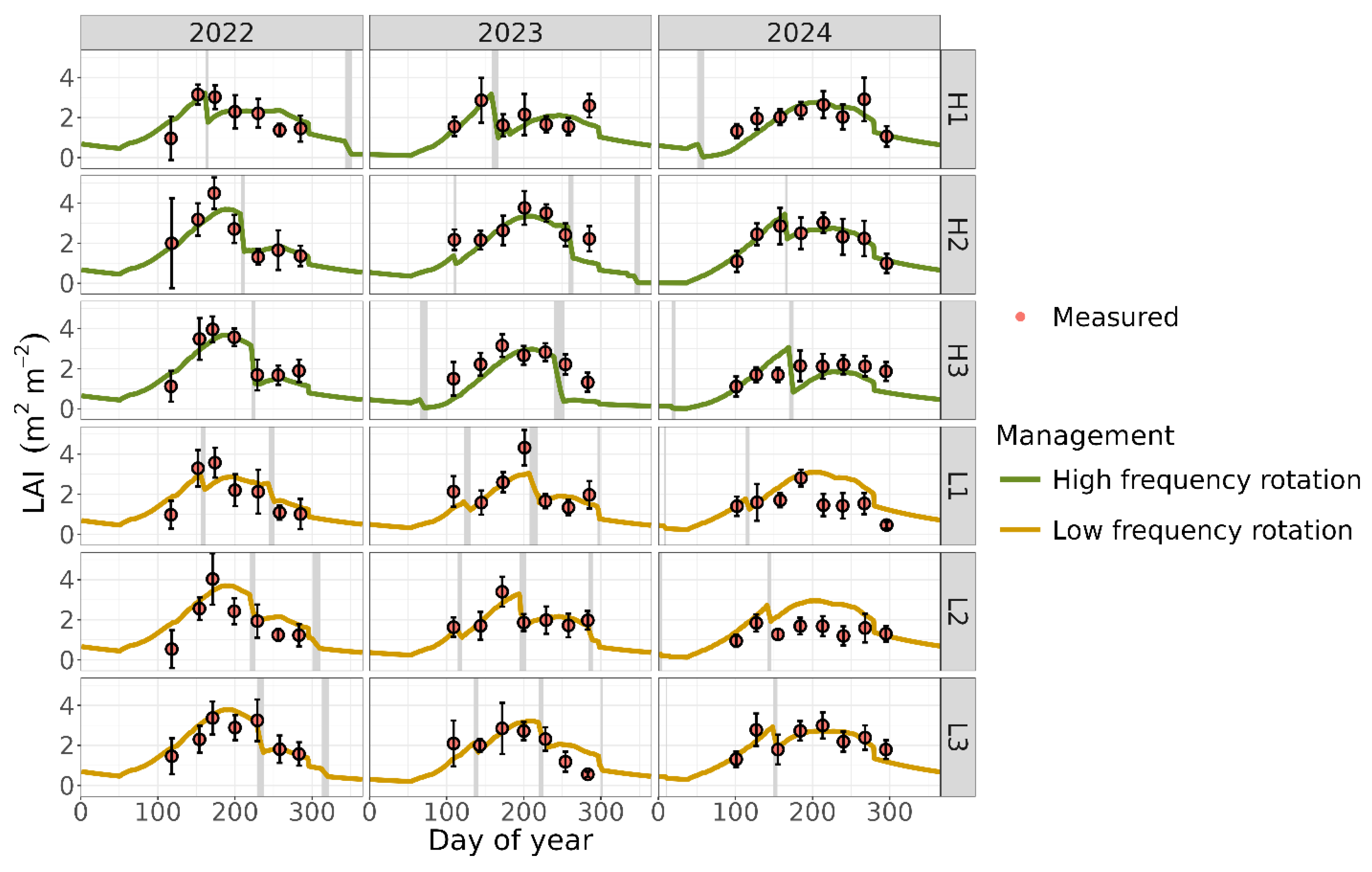
Figure 3.
Measured (dots) and simulated (lines) plant aboveground biomass for each treatment plot managed under high frequency rotation (HFR; replicate plots H1-H3) and low frequency rotation (LFR; replicate plots L1-L3) grazing, at the Coffey Ranch in south-central Oklahoma, USA. Gray shading indicates grazing events. Vertical bars represent the standard deviation of the mean for measured values (n = 6).
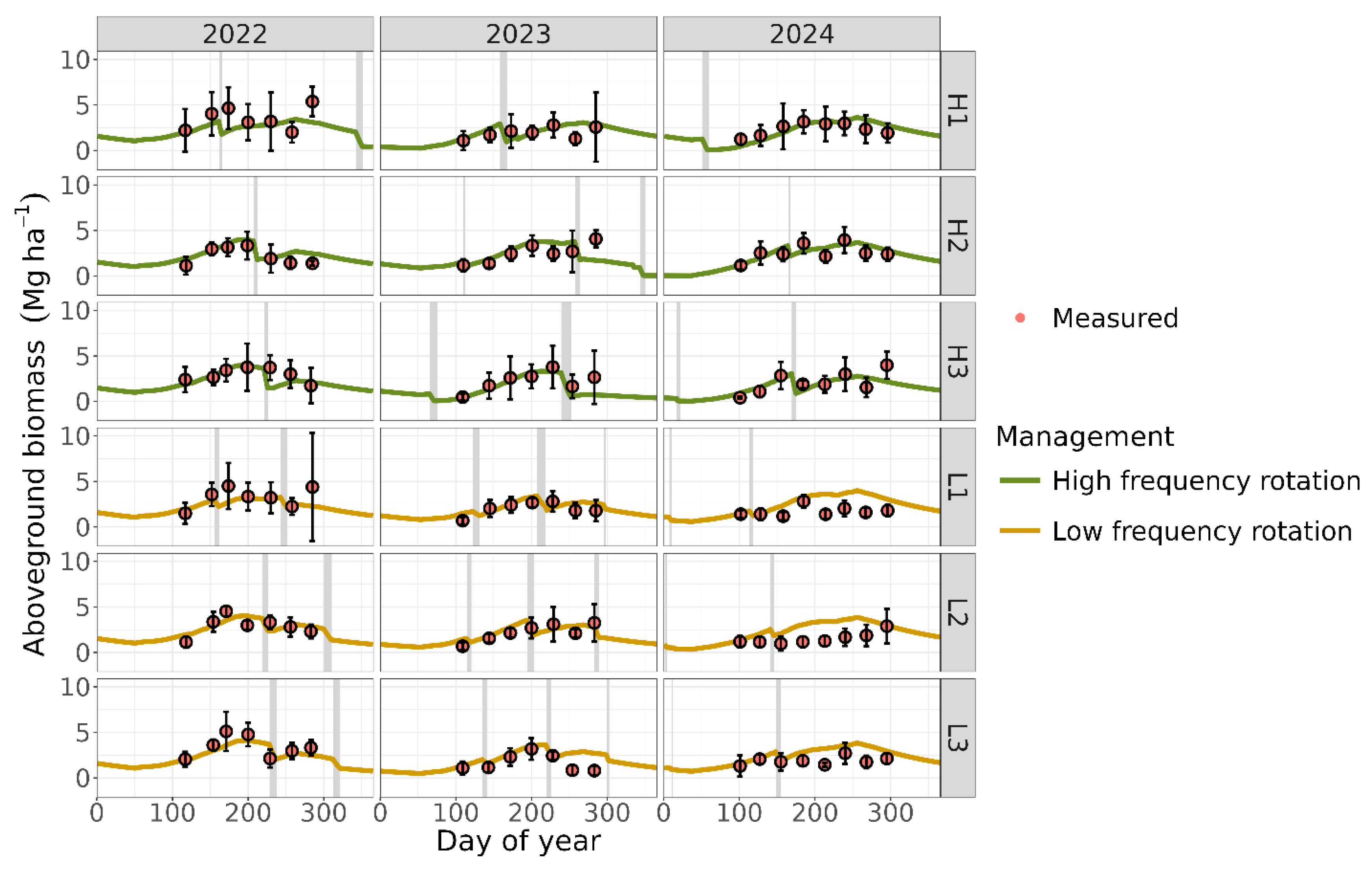
Figure 4.
Changes in vegetation indices and biomass with grazing as a function of distance to water for experimental plots L1 and L3 across different periods. Panels (a-c) show the calculated Sentinel-2 delta Enhanced Vegetation Index (ΔEVI) for two imagery dates prior to a grazing event: L1 (2022, DOY 149–139), L3 (2023, DOY 209–204), and L3 (2024, DOY 139–129). Panels (d-f) present MEMS 3.0-simulated delta Leaf Area Index (ΔLAI) for the same dates and plots. Panels (g-i) illustrate the calculated Sentinel-2 ΔEVI for one imagery date pre-grazing and another post-grazing: L1 (2022, DOY 164–149), L3 (2023, DOY 229–209), and L3 (2024, DOY 159–139). Panels (j-l) show MEMS 3.0-simulated ΔLAI for the same pre- and post-grazing dates. Panels (m-o) display the simulated proportion of grazed biomass among the simulated spatial units for the grazing periods. All dates are expressed as day of year (DOY). Color gradients in ΔEVI plots (a-c, g-i) represent the count of observations.
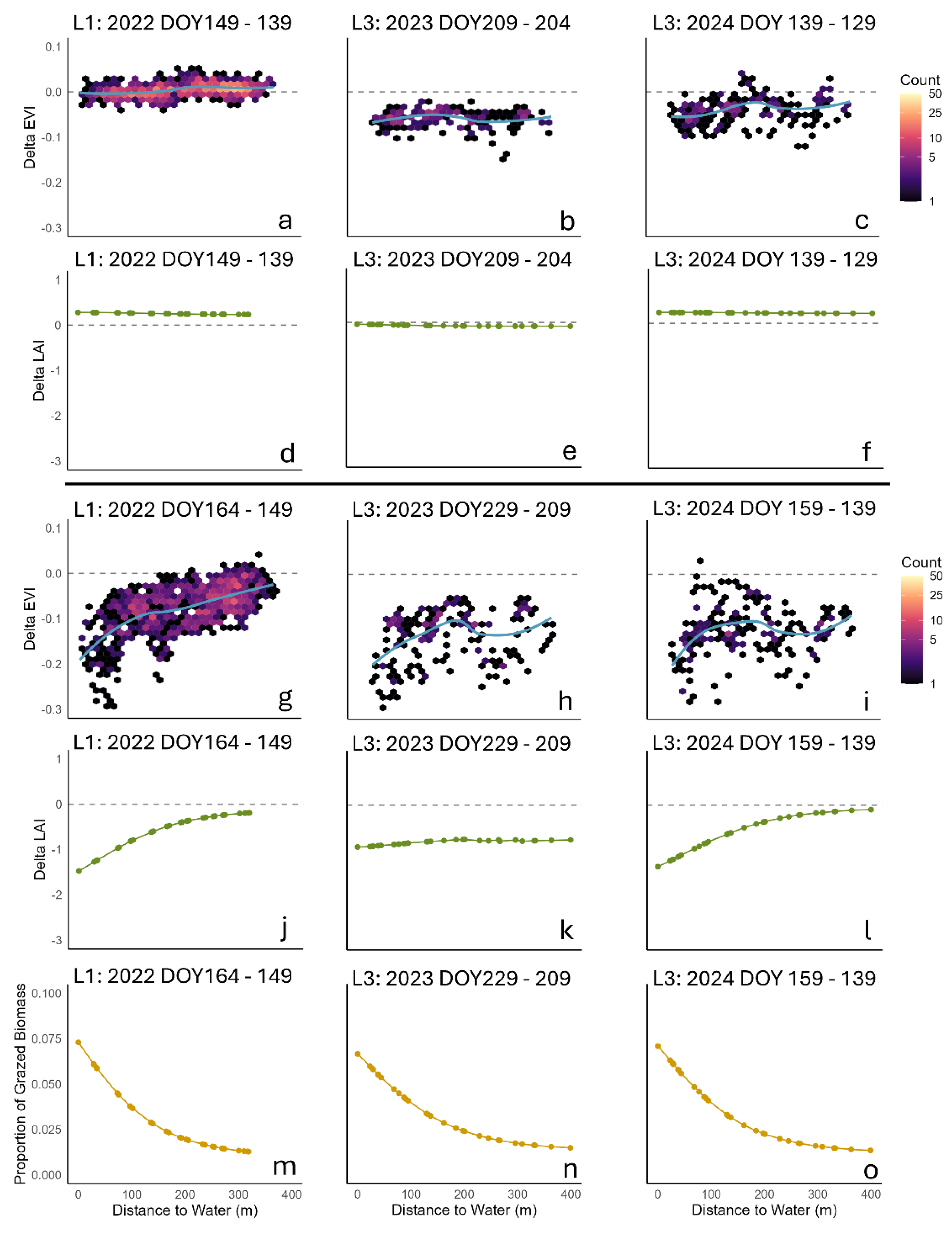
Figure 5.
Simulated yearly net primary productivity (NPP) averaging over all spatial units, comparing the impacts of three weather scenarios (simulations with repeated one year of weather for annual precipitation representing average, wet, and dry conditions), seven stocking rate scenarios [2 to 5 AU ha-1 with corresponding harvest efficiency (HE)], two schedule patterns (2 and 3 events in a year), and two grazing management types [low frequency rotation (LFR) and high frequency rotation (HFR)].
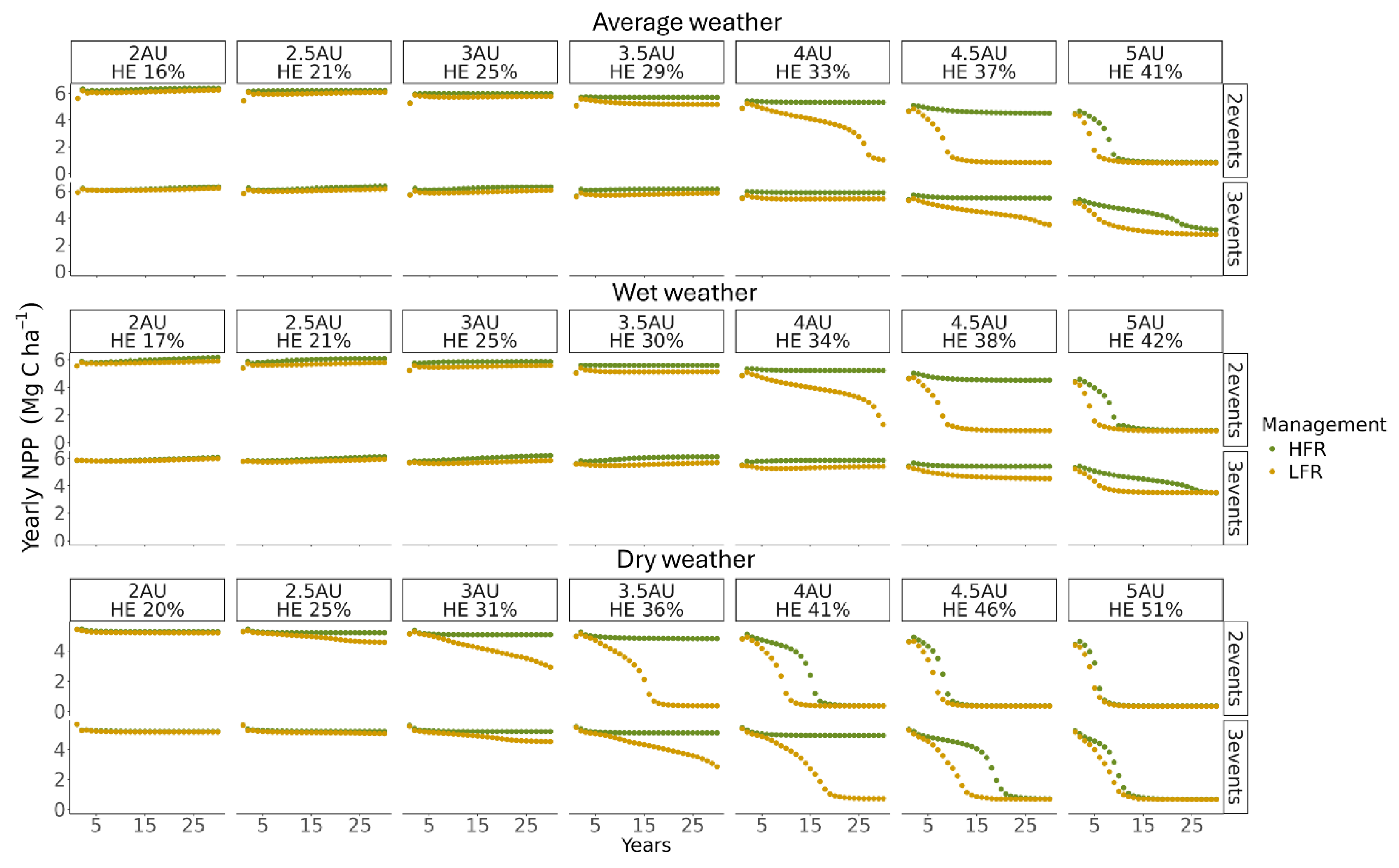
Disclaimer/Publisher’s Note: The statements, opinions and data contained in all publications are solely those of the individual author(s) and contributor(s) and not of MDPI and/or the editor(s). MDPI and/or the editor(s) disclaim responsibility for any injury to people or property resulting from any ideas, methods, instructions or products referred to in the content. |
© 2026 by the authors. Licensee MDPI, Basel, Switzerland. This article is an open access article distributed under the terms and conditions of the Creative Commons Attribution (CC BY) license (http://creativecommons.org/licenses/by/4.0/).
Copyright: This open access article is published under a Creative Commons CC BY 4.0 license, which permit the free download, distribution, and reuse, provided that the author and preprint are cited in any reuse.


