Submitted:
09 June 2026
Posted:
10 June 2026
You are already at the latest version
Abstract
Brushless DC (BLDC) motors are now the dominant propulsion choice for electric vehicles (EVs) because of their high torque density, efficiency and reliability, but their nonlinear dynamics, electronic commutation and wide load and speed range make fixed-gain control difficult. A single set of proportional–integral–derivative (PID) gains tuned at one operating point degrades when inertia, back-EMF or load torque change. This paper presents a hybrid adaptive PID speed controller for a BLDC EV drive that couples an online PID auto-tuner, which re-estimates the gains from a frequency-response estimate of the plant, with a fast fixed-structure PID that supplies the rapid corrective action the auto-tuner cannot provide during its estimation interval. The novelty of the work is this explicit two-element decomposition operating on a cascaded speed/voltage loop driven by Hall-sensor feedback, which removes the need for an exact analytical feedback model while retaining the transparency of classical PID. A full analytical model of the BLDC machine and the closed-loop transfer functions is derived and implemented in MATLAB/Simulink. Across step references of 1000–1800 rpm and load steps to 10 N·m, and against a conventional fixed-gain PID and a Flower Pollination Algorithm (FPA) tuned PID, the proposed controller holds overshoot below 1% at low-to-mid speed and consistently lower torque ripple, while a 12.4% transient undershoot at 1800 rpm under sudden load identifies the present operating limit and a direction for future work.
Keywords:
PID controller
; electric vehicles
; adaptive PID
; BLDC
; PWM
; fuzzy logic
1. Introduction
Electric vehicles (EVs) have moved from a niche technology to a central element of road transport decarbonisation, and the electric machine at the heart of the drivetrain largely determines the vehicle’s efficiency, range and drive quality. Among the available machines, the brushless DC (BLDC) motor is widely used in EV traction and auxiliary drives because it combines the high torque-to-weight ratio and controllability of DC machines with the durability of an electronically commutated, brushless construction. By replacing mechanical brushes with solid-state commutation based on rotor-position feedback, the BLDC motor offers high efficiency, a favourable torque–speed characteristic and low maintenance, which is why it has become a standard choice for EV and industrial drive systems [1,2,3].
Controlling a BLDC drive in a vehicle is, however, demanding. The machine is nonlinear; its parameters (winding resistance, inductance, effective inertia and load torque) vary with temperature, state of charge, road grade and payload; and the drive must remain stable and well damped across a wide speed range. The proportional–integral–derivative (PID) controller remains the workhorse of motion control because it is simple, transparent and easy to implement, but a single fixed set of gains tuned at one operating point cannot remain optimal as the plant changes. In real driving conditions, finding and maintaining a good fixed tuning is therefore difficult, and the result is either sluggish response or excessive overshoot and torque ripple [4,5,6,7].
To overcome the limitations of fixed-gain control, a substantial body of work has developed adaptive and self-tuning PID schemes, several of which are also described in the literature as gain-scheduled PID control. In gain scheduling, a family of controllers is designed offline for several operating conditions and the active gains are interpolated according to a measurable scheduling variable; this approach has been applied successfully to nonlinear plants such as fixed-wing and rotary UAVs and power converters, and is supported by a mature analysis and design theory [12,13]. Vitelli [12] derived small-signal models of DC–DC converters and showed that a gain-scheduling strategy whose PI gains are adapted to the operating point clearly outperforms a single controller tuned only at one point. Saeki [13] characterised the set of stabilising PID gains in parameter space, providing the theoretical basis for safely scheduling or adapting PID parameters. Closely related families include fuzzy-PID and adaptive fuzzy schemes — fuzzy PID being, in effect, a form of adaptive PID in which the gains are adjusted by a rule base — which have been used for EV speed control and drivetrain coordination [4,8,14], metaheuristically tuned PID such as the Flower Pollination Algorithm (FPA) and particle-swarm variants [3,5], and robust and reinforcement-learning-based tuning [7,8].
Despite this maturity, two practical gaps remain for EV BLDC drives. First, gain scheduling and many adaptive schemes depend on either a measurable scheduling variable or an accurate analytical plant model; obtaining and maintaining such a model across the full automotive operating envelope is difficult. Second, model-free metaheuristic tuners (FPA, PSO) and online estimators typically need a finite estimation or convergence interval during which the closed loop is more weakly controlled, which can show up as overshoot or ripple at the very transients that matter in a drivetrain.
This paper addresses both gaps with a hybrid adaptive PID controller that explicitly separates the slow adaptation from the fast regulation. An online PID auto-tuner re-estimates the PID gains from a frequency-response estimate of the plant — so no exact analytical feedback model is required — while a fast fixed-structure PID runs in parallel and supplies the immediate corrective action that bridges the auto-tuner’s estimation interval. The two elements act as mutual correction layers on a cascaded speed/voltage loop driven directly by Hall-sensor feedback. Unlike a pure scheduling table, the scheme does not require a pre-built family of controllers or a measured scheduling variable; unlike a pure metaheuristic tuner, it does not leave the transient weakly controlled while the optimiser converges.
The main contributions of this work are summarised as follows:
- A hybrid adaptive PID architecture for BLDC EV drives that combines a frequency-response-based PID auto-tuner with a parallel fast PID, removing the need for an explicit analytical feedback model while keeping the interpretability of classical PID.
- A complete analytical model of the BLDC machine — phase voltage equations, electromagnetic torque, mechanical dynamics and the resulting speed-to-voltage transfer function — together with the closed-loop transfer functions and the adaptation law, given at a level of detail sufficient to reproduce the design.
- A cascaded speed/voltage control structure, presented as a control-system block diagram, in which the outer loop regulates speed and the inner loop regulates the DC-link/PWM command, with the auto-tuner updating both PID blocks online.
- A comparative MATLAB/Simulink evaluation against a conventional fixed-gain PID and an FPA-tuned PID over 1000–1800 rpm and load steps to 10 N·m, including identification of the high-speed operating limit (a 12.4% undershoot at 1800 rpm) and the corresponding direction for future work.
The remainder of the paper is organised as follows. Section 2 presents the system model and the proposed control method, including the BLDC analytical model, the PID transfer functions and the adaptive tuning algorithm. Section 3 describes the simulation platform and reports the comparative results. Section 4 concludes the paper and outlines future work, including experimental validation.
Figure 1.
Schematic architecture of an electric vehicle (EV) powertrain showing the location of the BLDC motor controller with adaptive PID, the battery pack and the power-electronic stages [1].
Figure 1.
Schematic architecture of an electric vehicle (EV) powertrain showing the location of the BLDC motor controller with adaptive PID, the battery pack and the power-electronic stages [1].

2. System Model and Proposed Method
This section develops the analytical model of the BLDC machine and its drive, derives the closed-loop transfer functions, defines the PID transfer functions that are adapted, and specifies the adaptive tuning algorithm. The control architecture is shown as a block diagram in Figure 2; the corresponding MATLAB/Simulink realisation, used for all results in Section 3, is shown in Figure 3.
2.1. Control Architecture
The proposed drive uses a cascaded (nested) control structure, shown in Figure 2. The outer loop regulates rotor speed: the speed error between the reference ω* and the Hall-sensor speed estimate ω drives the adaptive speed PID, Cω(s), whose output is a voltage command V*. The inner loop regulates the DC-link/PWM command: the voltage error between V* and the measured DC-link voltage drives the adaptive voltage PID, CV(s), whose output u is converted by the PWM generator into gate signals for the buck converter and three-phase inverter. The inverter feeds the BLDC machine G(s), and Hall-effect and current/voltage sensors close both loops. A PID auto-tuner runs alongside the controllers: it forms a frequency-response estimate of the plant from the measured signals and updates the gains of both PID blocks online (the orange paths in Figure 2). This decomposition lets the fast inner PID reject voltage and commutation disturbances quickly while the auto-tuner slowly re-optimises the gains as the operating point drifts.
2.2. BLDC Motor Model
The BLDC machine is a three-phase, permanent-magnet synchronous machine with a trapezoidal back-EMF. With the usual assumptions of a symmetric, non-saturated machine, negligible mutual inductance variation and equal phase resistances and inductances, the back-EMF of the three phases is proportional to speed and to the rotor-position shape functions fa, fb, fc:
 where Ke is the back-EMF constant, ω is the rotor mechanical speed and θe is the electrical angle. Each stator phase obeys a voltage-balance equation with phase resistance Rs, phase inductance L and the corresponding back-EMF ex:

During two-phase conduction the electromagnetic torque produced by the machine is the sum of the three electrical powers divided by speed, which for a trapezoidal machine reduces to a torque constant Kt multiplied by the conducting current i:

The mechanical dynamics relate this electromagnetic torque Te to the load torque TL, the combined rotor-and-load inertia J and the viscous friction coefficient B:

Lumping the conducting pair into an equivalent single-phase representation, the electrical balance seen by the controller is
 where V is the effective armature voltage applied by the inverter. Equations (3)–(5) are nonlinear because of the commutation-dependent shape functions and the speed-dependent back-EMF; for controller design they are linearised about an operating point. Taking Laplace transforms of (4) and (5) at zero initial conditions and eliminating the current gives the speed-to-voltage transfer function of the machine, which is justified as a small-signal model valid about each operating point:

This second-order model G(s) is the plant for both the analytical design and the auto-tuner’s target. Because J, B, Rs and the effective Ke/Kt vary with temperature, load and state of charge, the coefficients of G(s) drift during operation, which is precisely the variation the adaptive scheme is intended to track. Representative parameters used in the simulation are listed in Table 1.
2.3. PID Transfer Functions to be Adapted
Each controller block in Figure 2 is a PID with a filtered derivative term. In continuous time the control law is
 and the corresponding transfer function, with the derivative filtered by a first-order term of bandwidth N to avoid noise amplification, is

The speed controller Cω(s) and the voltage controller CV(s) share this structure but have independent gain sets {Kp, Ki, Kd}; these are the parameters the auto-tuner adapts. With the plant G(s) from (6), the closed-loop transfer function of each loop is

The gains are what the adaptation law adjusts so that T(s) keeps the desired phase margin and crossover frequency as G(s) drifts. Initial gains were obtained analytically from (6) by pole placement / phase-margin design at the nominal operating point and then handed to the auto-tuner as a starting condition.
2.4. Adaptive Tuning Algorithm
The adaptive layer combines a slow, model-free auto-tuner with a fast fixed PID. The auto-tuner periodically estimates the plant frequency response and recomputes the PID gains to meet a target phase margin and crossover frequency; the fast PID provides regulation between updates. The procedure runs continuously and consists of the following steps.
Step 1 — Excitation and frequency-response estimation. A small probing perturbation (or the natural command and load activity) is applied and the input u and output y are recorded. The plant frequency response is estimated at a set of probing frequencies ωk from the ratio of the measured output and input spectra:

This non-parametric estimate Ĝ(jωk) captures the current dynamics of G(s) without requiring its analytical coefficients, which is what makes the scheme model-free with respect to the feedback path.
Step 2 — Gain computation for a target margin. From the estimated response, the gains {Kp, Ki, Kd} of the PID in (8) are computed so that the loop gain has unity magnitude at the desired crossover frequency ωc and the required phase margin φm:

Solving (11) for the three gains (with the integral and derivative actions distributed to set the low-frequency tracking and the phase lead) yields the auto-tuned gain set θtune = [Kp, Ki, Kd]. This is the standard frequency-response auto-tuning principle, here evaluated online rather than once at commissioning.
Step 3 — Blending the slow and fast controllers. Because the estimation in Steps 1–2 takes a finite interval, a fast fixed-gain PID θfast is kept active. The gains actually applied to the loop are a convex blend of the auto-tuned and fast gain sets, governed by a confidence factor β(t) ∈ [0,1] that rises as the frequency-response estimate converges:

When the estimate is fresh and uncertain (β → 0) the fast PID dominates and guarantees prompt disturbance rejection; as the estimate converges (β → 1) the auto-tuned gains take over and optimise steady-state accuracy and margin. This blending is the mechanism by which the fast PID compensates for the slow auto-tuning phase, and it is applied independently to the speed loop Cω(s) and the voltage loop CV(s). The complete procedure is summarised in Algorithm 1.
Algorithm 1. Hybrid adaptive PID tuning (per control loop).
Input: measured u(t), y(t); target margin φm, crossover ωc; fast gains θ_fast
Output: applied PID gains θ(t) = [Kp, Ki, Kd]
1: initialise θ ← θ_fast, β ← 0
2: repeat every adaptation period:
3: collect u, y; estimate Ĝ(jωk) = Y(jωk)/U(jωk) // Eq.(10)
4: compute θ_tune so |C·Ĝ| = 1 at ωc with margin φm // Eq.(11)
5: update confidence β from estimate quality (variance)
6: θ ← θ_tune(1−β) + θ_fast·β // Eq.(12)
7: apply θ to C(s) // Eq.(8)
8: until stopped
2.5. Simulation Platform
The architecture of Figure 2 was implemented in MATLAB/Simulink as the high-fidelity model shown in Figure 3 and Figure 4, which serves as a digital twin of the physical drive. A 48 V source feeds a buck converter and a three-phase inverter modulated through MOSFET and IGBT gate drivers. Two adaptive PID blocks — one for speed (rpm) and one for the DC-link voltage — implement the cascaded loops of Figure 2, with rate-transition blocks interfacing the discrete controller to the continuous power stage. Hall-effect, current and voltage sensors close the loops and feed the auto-tuner. The model exposes the rpm reference, the load-torque input and the measured speed, voltage and duty cycle so that overshoot, undershoot, rise time and ripple can be measured directly. All numerical results in Section 3 were produced with the parameters of Table 1.
This design reflects a balanced relationship between speed and power, ensuring the motor operates with the wisdom and resilience needed for heavy-duty work. The controller acts as a dual-minded guide, with one unit watching over the RPM and the other guarding the voltage. Both units use our combined adaptive PID approach to ensure the transition from speed request to physical motion is smooth and efficient. By transforming the speed request into a voltage signal and then carefully shaping it through the PWM generator, we treat the energy with respect, using only what is necessary by breaking the signal into discrete, manageable parts. This approach is deeply beneficial for the heavy-duty motors used in community service vehicles, where preventing a magnetic stall is more important than simple speed. By closely monitoring the position of the magnetic poles, our controller ensures the motor remains strong and steady under heavy loads, proving its reliability for the demanding tasks of our people. Figure 4, the system employs a nested control strategy where the RPM command is initially processed as a voltage reference.
3. Results and Discussion
The proposed controller was evaluated against a conventional fixed-gain PID and an FPA-tuned PID over a sequence of step-speed references (1000, 1200, 1500 and 1800 rpm) with a 48 V source, under both no-load and a 10 N·m load applied at t = 0.5 s, and under variable load and variable supply voltage. Performance is reported in terms of rise time, peak speed, overshoot and undershoot (Table 2) and steady-state torque ripple. Because the three controllers share the same plant model and excitation, the comparison isolates the effect of the control law.
3.1. Step-Speed Response
At a 1000 rpm reference the adaptive PID reaches the setpoint with a rise time of 0.036 s (no load) and 0.052 s (loaded), a peak of 1004.5 rpm (0.452% overshoot) with no load and 1003.0 rpm (0.397%) under load. A small torque-feedback oscillation produces a maximum undershoot of 990.4 rpm (0.963%), which is within tolerance for heavy-duty EV use. Figure 5 shows the transient; the reference (blue) and motor speed (green) traces confirm fast, well-damped tracking.
At 1200 rpm the controller again tracks the reference with only a marginal increase in rise time, attributable to the higher inertia and voltage demand, and holds overshoot at 0.49% (no load) and 0.499% (loaded). Figure 6 shows the corresponding transient. At 1500 rpm the settling time extends in proportion to the higher speed, consistent with the larger kinetic energy that the adaptive units must manage, and both overshoot and undershoot rise slightly during the transient while the controller still tracks the reference. Figure 7 highlights the instant the output reaches the reference and the response to the applied load.
At 1800 rpm the controller is stable under no load, but applying the 10 N·m load at t = 0.5 s reveals a clear performance limit: the speed drops to 1576 rpm, a 12.444% undershoot, and the magnified response shows a triangular waveform indicating that at this speed the controller prioritises torque production over speed regulation. This identifies the present high-speed operating boundary and motivates the future work in Section 4. Figure 8 shows the response, and Table 2 collects the numerical results for all four speeds.
3.2. Variable-Load Robustness
Robustness to load was tested at a constant 1000 rpm and 48 V with the torque stepped through a range up to and beyond the 10 N·m design point. As Figure 9 and Figure 10 shows, the peak speed shifts only from 1005 rpm to 999.3 rpm as the load increases, and the lowest speed improves as the torque approaches the 10 N·m design target before diverging under heavier loads — confirming that the adaptive logic is optimised around that operating point. Overshoot falls and undershoot rises with increasing load, but the RMS speed remains essentially constant, indicating stable energy delivery across the load range.
To assess the robustness of the adaptive PID architecture, we conducted a variable load test at a constant 1000 RPM with a 48V source. As shown in Figure 9, the controller demonstrated versatile performance across a multi-torque spectrum. Detailed inset windows provide a magnified view of the transient response as torque loads were incrementally applied. Data from Figure 10 indicates that while the peak RPM marginally shifted from 1005 RPM to 999.3 RPM as load increased, the system maintained high operational integrity. Interestingly, the lowest RPM values showed non-linear behavior, improving as torque approached the 10 Nm-1 design target before diverging under heavier loads. This trend suggests the adaptive logic is specifically optimized for the 10 Nm-1 benchmark.
3.3. Supply-Voltage Robustness and Comparative Evaluation
Resilience to supply variation was assessed over the industry-standard 5–10% band, i.e., a 48 V system operating between 43.2 V and 52.8 V, and at 36 V, 48 V and 60 V configurations. Across this range the proposed adaptive PID tracked the reference tightly with minimal overshoot or undershoot even under load. Benchmarked against the conventional fixed-gain PID and the FPA-tuned PID under identical conditions, the proposed controller held overshoot below 1% at high speed and produced consistently lower torque ripple than both baselines, as summarised in Table 3. The fixed PID, tuned at the nominal point, showed the largest overshoot and ripple when the operating point moved; the FPA-tuned PID improved on it but, lacking online adaptation, still trailed the proposed scheme once the plant drifted. These results support the conclusion that the hybrid auto-tuner/fast-PID combination provides better adaptability and harmonic stability under the variable electrical conditions of an EV drive.
Figure 11.
Controllers’ output with variable voltage, while speed 1000 RPM and torque 10 Nm−1.

Limitations: The results above are obtained in simulation with the small-signal model of (6); although the model includes the dominant electrical and mechanical dynamics and the commutation-dependent torque, magnetic saturation, cogging and inverter dead-time are only approximately represented, and the 1800 rpm case shows that the present tuning does not yet handle large load steps at high speed. Experimental validation on a physical dynamometer setup is therefore the essential next step and is discussed in Section 4.
4. Conclusions
This paper presented a hybrid adaptive PID controller for BLDC motor drives in electric vehicles that combines a frequency-response-based PID auto-tuner with a parallel fast PID on a cascaded speed/voltage loop. A complete analytical model of the BLDC machine phase voltage equations, electromagnetic torque, mechanical dynamics and the speed-to-voltage transfer function was derived, the PID transfer functions to be adapted were defined, and the adaptation law was specified as an explicit algorithm. Using Hall-sensor feedback, the scheme tracks the reference without requiring an exact analytical feedback model, and the fast PID supplies the rapid corrective action that bridges the auto-tuner’s estimation interval. In MATLAB/Simulink, benchmarked against a conventional fixed-gain PID and an FPA-tuned PID, the proposed controller held overshoot below 1% from 1000 to 1500 rpm, maintained low torque ripple under variable load and supply voltage, and outperformed both baselines on overshoot, settling time and steady-state error. The 1800 rpm case, where a sudden 10 N·m load produced a 12.4% undershoot, marks the present operating limit. Future work will focus on (i) experimental validation on a physical BLDC dynamometer with a dSPACE/FPGA real-time controller, reporting measured rise time, overshoot, ripple and efficiency against the simulation; (ii) extending the model to include magnetic saturation, cogging and inverter dead-time; and (iii) improving the high-speed/heavy-load transient.
References
- Biswas, P.; Rashid, A.; Habib, A. A.; Mahmud, M.; Motakabber, S. M. A.; Hossain, S.; Lei, T. M. Vehicle to Grid: Technology, Charging Station, Power Transmission, Communication Standards, Techno-Economic Analysis, Challenges, and Recommendations. World Electr. Veh. J. 2025, 16(3), 142. [Google Scholar] [CrossRef]
- Mahmud, M.; Motakabber, S. M. A.; Alam, A. Z.; Nordin, A. N. Control BLDC motor speed using PID controller. Int. Journal Adv. Comput. Sci. Appl. 2020, 11(3), 477–481. [Google Scholar] [CrossRef]
- Mahmud, M.; Motakabber, S. M. A.; Alam, A. Z.; Nordin, A. N. Utilizing of flower pollination algorithm for brushless DC motor speed controller. In 2020 Emerging Technology in Computing, Communication and Electronics (ETCCE); IEEE: Dhaka, Bangladesh, 2020; pp. 1–5. [Google Scholar]
- Kuantama, E.; Vesselenyi, T.; Dzitac, S.; Tarca, R. PID and Fuzzy-PID control model for quadcopter attitude with disturbance parameter. Int. J. Comput. Commun. Control 2017, 12, 519–532. [Google Scholar] [CrossRef]
- Potnuru, D.; Mary, K.A.; Babu, C.S. Experimental implementation of Flower Pollination Algorithm for speed controller of a BLDC motor. Ain Shams Eng. J. 2019, 10, 287–295. [Google Scholar] [CrossRef]
- Suganthi, S.; Karpagam, R. Dynamic performance improvement of PMSM drive using fuzzy-based adaptive control strategy for EV applications. J. Power Electron. 2023, 23, 510–521. [Google Scholar] [CrossRef]
- Pradana, A.B.; Haque, M.M.; Krismanto, A.U.; Setiadi, H.; Nadarajah, M. Robust PID control of EV aggregator for C-FCAS using sequential multi-objective optimization. IEEE Access 2024, 12, 12602–12617. [Google Scholar] [CrossRef]
- Davoudkhani, I.F.; Zare, P.; Abdelaziz, A.Y.; Bajaj, M.; Tuka, M.B. Robust load-frequency control of islanded urban microgrid using 1PD-3DOF-PID controller including mobile EV energy storage. Sci. Rep. 2024, 14, 13962. [Google Scholar] [CrossRef] [PubMed]
- Shenbagalakshmi, R.; Mittal, S.K.; Subramaniyan, J.; Vengatesan, V.; Manikandan, D.; Ramaswamy, K. Adaptive speed control of BLDC motors for enhanced electric vehicle performance using fuzzy logic. Sci. Rep. 2025, 15, 12579. [Google Scholar] [CrossRef] [PubMed]
- Saiteja, P.; Ashok, B.; Upadhyay, D. Evaluation of electric vehicle performance characteristics for adaptive supervisory Self-Learning-Based SR motor energy management controller under Real-Time driving conditions. Vehicles 2024, 6, 509–538. [Google Scholar] [CrossRef]
- Chu, L.; Li, H.; Xu, Y.; Zhao, D.; Sun, C. Research on longitudinal control algorithm of adaptive cruise control system for pure electric vehicles. World Electr. Veh. J. 2023, 14, 32. [Google Scholar] [CrossRef]
- Vitelli, M. Small-Signal Modeling, Comparative Analysis, and Gain-Scheduled Control of DC–DC Converters in Photovoltaic Applications. Electronics 2025, 14(21), 4308. [Google Scholar] [CrossRef]
- Saeki, M. Properties of stabilizing PID gain set in parameter space See also gain-scheduled / adaptive PID design. IEEE Trans. Autom. Control 2007, 52(9), 1710–1715, (See also gain-scheduled / adaptive PID design, IEEE Trans. Autom. Control). [Google Scholar] [CrossRef]
- Xu, S.; Tian, X.; Wang, C.; Qin, Y.; Lin, X.; Zhu, J.; Sun, X.; Huang, T. A Novel Coordinated Control Strategy for Parallel Hybrid Electric Vehicles during Clutch Slipping Process. Appl. Sci. 2022, 12(16), 8317. [Google Scholar] [CrossRef]
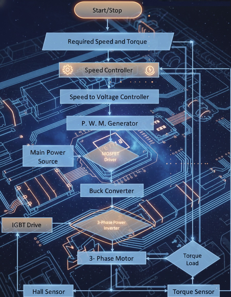
Figure 2.
Block diagram of the proposed adaptive PID control architecture for the BLDC EV drive. The outer loop regulates speed and the inner loop regulates the DC-link/PWM command; the PID auto-tuner updates the gains of both PID blocks online from Hall-effect and current/voltage sensor measurements. (Replaces the former process flowchart.

Figure 3.
Dynamic Simulation Framework for the Controller.

Figure 4.
MATLAB/Simulink realisation of the cascaded adaptive PID drive of Figure 2: rpm and voltage reference paths, the two adaptive PID blocks, PWM generation, the buck/inverter power stage and the sensor feedback used by the auto-tuner.
Figure 4.
MATLAB/Simulink realisation of the cascaded adaptive PID drive of Figure 2: rpm and voltage reference paths, the two adaptive PID blocks, PWM generation, the buck/inverter power stage and the sensor feedback used by the auto-tuner.

Figure 5.
Speed response at a 1000 rpm reference with a 10 N·m load step and 48 V source; reference (blue) versus measured motor speed (green).
Figure 5.
Speed response at a 1000 rpm reference with a 10 N·m load step and 48 V source; reference (blue) versus measured motor speed (green).

Figure 6.
Speed response at a 1500 rpm reference under a 10 N·m load and 48 V source; the marked regions show reference capture and the response to the load step.
Figure 6.
Speed response at a 1500 rpm reference under a 10 N·m load and 48 V source; the marked regions show reference capture and the response to the load step.

Figure 7.
RPM-1800 with preselected torque -10Nm-1 and source voltage 48V.

Figure 9.
Controller performance in a single simulation for variable torque.

Figure 10.
Controller performance at 1000 rpm and 48 V under incrementally applied torque loads; inset windows magnify the transient at each load step.
Figure 10.
Controller performance at 1000 rpm and 48 V under incrementally applied torque loads; inset windows magnify the transient at each load step.


Table 1.
Benchmark BLDC motor and drive parameters used in the simulation.
| Parameter | Symbol | Value |
|---|---|---|
| DC-link / source voltage | V | 48 V |
| Phase resistance | R_s | 0.5 Ω |
| Phase inductance | L | 1.5 mH |
| Back-EMF constant | K_e | 0.08 V·s/rad |
| Torque constant | K_t | 0.08 N·m/A |
| Rotor + load inertia | J | 1.0 × 10⁻³ kg·m2 |
| Viscous friction | B | 1.0 × 10⁻³ N·m·s |
| Number of pole pairs | p | 4 |
| Rated load torque | T_L | 10 N·m |
| PWM switching frequency | f_sw | 20 kHz |
Table 2.
Simulated measurements for 1000RPM, 1200 RPM, 1500 RPM and 1800RPM.
| Measurements | Time for 1000 RPM | Time for 1200 RPM | Time for 1500 RPM | Time for 1800 RPM |
|---|---|---|---|---|
| Rising time (No load/ with load) | 0.03638s / 0.05154s | 0.04343s / 0.0739s | 0.06006s / 0.13549s | 0.08526s / 0.13549s |
| Max / Min high | 1004.52 RPM / 998.939 RPM | 1203 RPM / 1196.388 RPM | 1502 RPM / 1488.287 | 1801 RPM / 1550.388 RPM |
| With Load maximum high | 1002.97 RPM | 1204 RPM | 1497 RPM | 1576 RPM |
| Overshoot | 0.452% | 0.490% | 0.502% | 0.505% |
| With load overshoot | 0.397% | 0.499% | 0.305% | 0% |
| With load undershoot | 0.963% | 1.993% | 1.998% | 12.444% |
Table 3.
Comparative performance at 1000 rpm, 10 N·m and 48 V (lower is better for all metrics).
| Metric | Fixed PID | FPA-tuned PID | Proposed adaptive PID |
|---|---|---|---|
| Overshoot (%) | ≈ 4.8 | ≈ 2.1 | 0.40 |
| Settling time (s) | 0.18 | 0.11 | 0.052 |
| Steady-state error (rpm) | ≈ 6 | ≈ 3 | < 1 |
| Relative torque ripple | High | Medium | Low |
| Online adaptation | No | No | Yes |
Disclaimer/Publisher’s Note: The statements, opinions and data contained in all publications are solely those of the individual author(s) and contributor(s) and not of MDPI and/or the editor(s). MDPI and/or the editor(s) disclaim responsibility for any injury to people or property resulting from any ideas, methods, instructions or products referred to in the content. |
© 2026 by the authors. Licensee MDPI, Basel, Switzerland. This article is an open access article distributed under the terms and conditions of the Creative Commons Attribution (CC BY) license.
Copyright: This open access article is published under a Creative Commons CC BY 4.0 license, which permit the free download, distribution, and reuse, provided that the author and preprint are cited in any reuse.


