Submitted:
09 February 2026
Posted:
11 February 2026
You are already at the latest version
Abstract
Parameter estimation for biochemical reaction networks is computationally demanding, especially for systems with oscillatory nonlinear dynamics, where standard iterative optimization strategies, including genetic algorithms, often struggle with prohibitive computational costs. We introduce an efficient parameter estimation framework that combines a real-coded genetic algorithm with a novel adaptive simulation termination strategy. This strategy defines a time-dependent termination boundary based on population quantiles, which is permissive during early transients and becomes progressively stricter as simulations advance, explicitly accounting for the temporal structure of oscillatory behavior. Crucially, this mechanism facilitates the efficient identification and early simulation termination of poor parameter candidates, thus avoiding the computational expense of full-horizon simulations. The framework further integrates global exploration with the modified Powell method for rapid local refinement. Numerical experiments on two benchmark oscillatory models—the Lotka–Volterra and Goodwin oscillators—demonstrate that the framework reduces computational cost by approximately 30%–50% compared to a baseline GA without this strategy. For the parameter-sensitive Goodwin model, the framework efficiently identifies candidates evolving toward damped oscillations caused by subtle parameter variations. Sensitivity analysis also confirms robustness across diverse hyperparameter settings, indicating that adaptive simulation termination provides a practical acceleration mechanism for inverse problems in systems biology where iterative objective-function evaluation dominates runtime.
Keywords:
systems biology
; inverse problems
; parameter estimation
; genetic algorithms
1. Introduction
Parameter estimation for biochemical reaction networks is a fundamental challenge in systems biology [1,2,3,4,5]. Ordinary differential equation (ODE) models, including those based on Michaelis–Menten kinetics and their extensions, are commonly used to describe nonlinear dynamical systems such as enzymatic reactions, metabolic pathways, and cellular signaling processes. The predictive accuracy of these models critically depends on accurate kinetic parameters—such as reaction rate constants and affinity coefficients—derived from experimentally observed time-course data. Because many kinetic parameters cannot be measured directly, computational inference is essential. However, solving this inverse problem remains difficult owing to strong nonlinearity, complex interactions among parameters, and limited observability of internal system states.
Evolutionary computation methods, particularly real-coded genetic algorithms (GAs), have been widely applied to parameter estimation in biochemical reaction and gene regulatory networks owing to their robustness in nonconvex, multimodal search landscapes. Real-coded GAs are especially advantageous when gradient information is unavailable, a common scenario in large-scale biochemical reaction networks. In our previous studies, we demonstrated the effectiveness of real-coded GAs for these tasks; and then we proposed hybrid strategies in which a real-coded GA first identifies promising regions of the search space, followed by rapid local refinement using the modified Powell method [6,7,8,9,10,11,12,13,14,15].
Although standard optimization strategies based on iterative solution methods including GAs can improve practical convergence, they remain computationally demanding. A major bottleneck arises because they require many fitness evaluations, each involving numerical integration of nonlinear ODE systems across all experimental conditions. This burden is particularly pronounced when time-course data span long horizons or multiple initial conditions must be considered. In highly multimodal landscapes, substantial computational effort is often wasted evaluating clearly inferior candidates, especially during the early stages of the search. The Goodwin oscillator illustrates typical nonlinear oscillatory dynamics in biochemical reaction networks: while it can exhibit stable sustained oscillations (limit cycles) over long periods, slight parameter variations may produce weakly damped oscillations with gradual amplitude decay (asymptotic stability) [16,17,18,19,20]. Accurately distinguishing such damped behavior from truly sustained oscillations generally requires long-horizon simulations and detailed inspection of the resulting time-course data, further increasing computational cost. These challenges highlight the need for strategies that can efficiently eliminate parameter candidates prone to gradually decaying oscillatory behavior.
To address this limitation, we use the sequential structure of time-course data to accelerate optimization. During numerical simulation, poor parameter candidates often diverge considerably from experimental observations at early time points, long before the full simulation horizon is reached. This suggests that full-horizon simulations are not always necessary to eliminate clearly inferior candidates. However, oscillatory biochemical reaction networks present a specific challenge: early simulation phases often reflect transient responses that differ from the steady oscillations observed experimentally. As a result, candidates that poorly match early data may still reproduce the correct long-term oscillatory behavior, while others that initially align well may fail to sustain oscillations. Therefore, naive early termination based only on initial errors risks discarding potentially valid solutions (false negatives), whereas standard full-horizon evaluations expend substantial resources on candidates that gradually decay.
In this study, we propose an efficient parameter estimation framework for oscillatory biochemical reaction networks that incorporates a novel adaptive simulation termination strategy. The framework combines three key components: (i) a real-coded GA for global exploration of parameter space, (ii) a local optimization scheme based on the modified Powell method for rapid, gradient-free convergence, and (iii) an adaptive termination mechanism that evaluates ODE simulations sequentially, discarding candidates exhibiting persistent discrepancies before completing full-horizon simulations. The rejection criterion is transient-tolerant but progressively stricter, making it particularly well suited for estimating parameters that govern nonlinear oscillatory dynamics and for distinguishing sustained oscillations from weakly damped ones.
The proposed framework naturally accommodates multiple experimental conditions, such as varying initial concentrations or external perturbations, by defining the objective function as an aggregated, normalized error across all conditions and observables. Optimization is performed in a log-transformed parameter space to enforce positivity and stabilize the search across heterogeneous parameter scales. In the GA stage, a one-generation lag and a reference retention rule decouple boundary updates from candidate evaluation and prevent overly aggressive tightening when no valid offspring is produced. By reducing the average cost of objective-function evaluation through adaptive termination, this approach provides a scalable and practical iterative solution for parameter estimation in computationally demanding oscillatory biochemical reaction networks.
2. Proposed Framework
2.1. Problem Formulation
We consider a biochemical reaction network consisting of n chemical species governed by p unknown kinetic parameters. Let denote the vector of species concentrations at time t, and let denote the vector of kinetic parameters to be estimated. These parameters satisfy a component-wise positivity constraint:
Experiments are performed under multiple conditions indexed by (e.g., different initial concentrations or external perturbations). For each condition c, the system dynamics are given by
Here, represents the reaction kinetics, denotes condition-specific inputs, and is the corresponding initial state.
Let denote the experimental value of the k-th observable at time under condition c, and let denote the corresponding simulated value obtained by numerically solving Equation (2). We define the objective function as the aggregated, normalized absolute relative error over all conditions, observables, and time points:
Here, is the number of observables and is the number of observation time points for condition c.
To avoid numerical instability when experimental observations are close to zero, we introduce a stabilization constant in the denominator via , thereby preventing excessively large contributions when . In this near-zero regime, the normalized error behaves similarly to an absolute error scaled by , providing a smooth and practical way to handle zero or near-zero measurements without excluding them. In our experiments, we set
This stabilizes the objective function while leaving the relative-error behavior unchanged for typical observation magnitudes. In practice, results are generally insensitive to the accurate value of as long as it is sufficiently small, because mainly affects the low-signal regime .
The parameter estimation problem is formulated as
Remarks:
is highly nonlinear, nonconvex, and typically multimodal owing to nonlinear reaction kinetics and strong parameter interactions. Moreover, each evaluation of requires numerically solving Equation (2) for all experimental conditions, which can be computationally expensive.
2.2. Log-Transformed Parameterization
To handle positivity, optimization is performed in log space. Introduce via
This transformation enforces by construction, thereby eliminating the need for explicit inequality constraints. The logarithmic parameterization (i) improves scaling when parameters span multiple orders of magnitude, (ii) enhances numerical stability during ODE simulations, and (iii) aligns naturally with relative-error objectives such as Equation (3), where proportional deviations are meaningful. All evolutionary operations and local refinements are performed in -space, while model simulations use .
2.3. Global Exploration Using a GA
Global exploration is performed using a real-coded GA in log space. Individuals represent , and offspring are generated by Adaptive Real-coded Ensemble Crossover (AREX). We employ the Just Generation Gap (JGG) scheme with a population of size N at generation g [13,14,15,21,22].
- Offspring generation (AREX): In each generation, offspring are generated in -space using AREX with parents selected from . Each offspring is assigned a fitness value, evaluated as using either full-horizon simulation (baseline) or adaptive termination (proposed; Section 2.5).
- Generational replacement (JGG with partial replacement): In JGG, only a subset of parents is replaced in each generation. The parents selected for AREX are treated as replacement targets. After evaluating all offspring, we collect the subset of valid offspring for which the simulation is completed over the full horizon, and defineWe then perform partial replacement by: (i) sorting the target parents by fitness (worst first); (ii) sorting by fitness (best first); and (iii) replacing the worst r target parents with the best r valid offspring to form .
2.4. Local Refinement Using the Modified Powell Method
After the GA stage terminates, local refinement is performed using the modified Powell method [23], a derivative-free optimizer that often achieves fast local convergence. To control computational cost, Powell refinement is launched from only the top-ranked K GA individuals, balancing refinement quality and runtime. The modified Powell method is well-suited for this task because it has a proven track record in parameter estimation for biochemical reaction networks.
2.5. Partial Objective for Adaptive Simulation Termination
To reduce computational cost, the objective function in Equation (3) is evaluated incrementally over observation indices. At index j, a partial objective is calculated using only observations up to . For simplicity, we assume aligned observation indices in each model, i.e., , and the index j is shared across conditions:
The full objective function corresponds to . During numerical integration of Equation (2), the solver advances sequentially in time, and is updated at each observation time . If the partial objective exceeds the termination boundary at some index , numerical integration is terminated, and the candidate is rejected. For candidates rejected at , partial objectives at later indices are treated as undefined (missing) rather than assigned artificially large values, preventing distortion of population-level statistics used for thresholding.
2.6. Quantile-Based Reference and Updating Strategy
2.6.1. Trade-Offs and Strategies for Oscillatory Systems
The update schedule for the termination reference creates a trade-off between computational savings and robustness. Frequent updates can tighten thresholds quickly and improve efficiency, whereas delayed updates reduce false negatives and help maintain population diversity (Table 1). This balance is especially important for oscillatory biochemical reaction networks, where early phases are dominated by transients. Even if candidates show large mismatches initially, they may still develop into sustained oscillations over time.
Accordingly, we use a time-indexed, quantile-based reference designed for oscillatory dynamics. We define reference values for each observation index j and update the vector (and thus ) once per generation from the post-replacement population. This allows the termination boundary to adapt to the temporal evolution of the system:
- Early phases (transient): the population distribution is broad, i.e., partial fitness values have a wide range, yielding permissive thresholds that tolerate transient deviations.
- Late phases (stabilized): the population distribution becomes more concentrated, leading to stricter thresholds.
The thresholds are defined relative to the population distribution rather than based on a single best individual. Using quantile-based references preserves candidates that exhibit large transient deviations but eventually converge to sustained oscillations, while efficiently rejecting candidates that deviate persistently.
2.6.2. Population-Based Update with Generation Lag
We first perform a warm-up evaluation on the initial population without adaptive termination so that all individuals have full-horizon fitness values, ensuring that the initial quantiles are well defined. In each subsequent generation, we calculate quantile references for all indices from the post-replacement population:
The termination boundary is
where is a tolerance factor and controls the rate at which the tolerance decreases. To avoid circular dependence within a generation, a one-generation lag is used: offspring in generation g are evaluated using , and a candidate is early rejected at index j if
If no valid offspring is obtained (i.e., , hence ), no replacement occurs, and the references are retained:
After offspring evaluation and replacement, the updated references and are stored and used in generation . JGG partial replacement ensures that the population size remains N. Together with the warm-up evaluation at , the quantiles in Equation (9) remain well defined. For GA ranking and selection, rejected candidates are assigned a fixed penalized fitness and treated as invalid offspring, while quantile references are calculated from the post-replacement population (Equation (9)) and remain unaffected by the penalized values.
To provide intuition, Figure 1 visualizes partial fitness trajectories during evaluation. The green line represents the boundary , which is designed to be permissive early and progressively stricter over time. The red trajectories correspond to candidates that deviate substantially and are terminated early, avoiding wasteful full-horizon simulations. The blue trajectories correspond to promising candidates that remain below the boundary. Importantly, the relaxed early threshold (small ) acts as a buffer that tolerates transient errors inherent to oscillatory dynamics, reducing the risk of early termination for valid solutions (false negatives).
3. Numerical Experiments
3.1. Test Models and Synthetic Data
We evaluate the proposed framework on two benchmark models: (a) an oscillatory mass-action system (Lotka–Volterra predator–prey model) [24,25], and (b) an oscillatory biochemical feedback model (Goodwin oscillator) [16,17,18,19,20].
The Lotka–Volterra model serves as a canonical, fully observed oscillatory benchmark in theoretical population dynamics, whereas the Goodwin oscillator is a prototypical negative-feedback biochemical oscillator, widely used as a minimal model for gene-regulatory rhythms.
- (a)
- Lotka–Volterra (fully observed)
Consider the reaction scheme , yielding:
Here, and denote prey and predator concentrations. The parameter vector is , with ground-truth values . Two experimental conditions () are used with initial states and . All state variables are observed: .
- (b)
- Goodwin oscillator (partially observed)
We use the Goodwin model:
with the Hill coefficient fixed at to ensure sustained oscillations [18,19]. The parameter vector is , with ground-truth values and . Two experimental conditions () are used with initial states and . Only the third state variable is observed: . However, although only is observed, we show that the framework remains capable of parameter estimation under this partial observability.
Synthetic data are generated by numerically solving the ODEs using the ground-truth parameters and specified initial conditions. Noise-free observations are used to ensure a fair evaluation under identical settings. For both the Lotka–Volterra and Goodwin models, observations are sampled uniformly at 100 post-initial time points over (excluding the initial state at ), resulting in a total of 200 observations across the two initial conditions.
3.2. Compared Frameworks and Settings
We compare two frameworks under identical parameter bounds, optimization budgets, and solver settings, with the only difference being whether adaptive termination is applied during evaluation.
- Baseline (GA + Powell, full-horizon simulation): A real-coded GA explores the log-transformed parameter space, followed by local refinement using the modified Powell method. Each candidate is evaluated with the full-horizon objective (Equation (3)).
- GA settings: The population size is ; offspring are generated per generation using AREX with parents. The GA runs for generations with JGG partial replacement (Equation (7)). In both models, each kinetic parameter is constrained to lie between and 10 times its ground-truth value . All GA operations are performed in the log-transformed parameter space. The penalized fitness for rejected candidates is set to .
- Powell method settings: After the GA terminates, the modified Powell method is applied, starting from the top GA individuals ranked by the full objective . Each Powell run stops when improvements fall below a specified tolerance or when a maximum number of objective evaluations is reached; these stopping criteria are the same for both frameworks. During Powell refinement, the adaptive termination boundary is held fixed at the final GA boundary .
- Adaptive termination settings: Unless otherwise stated, we use quantile level , tolerance factor , and decay rate in Equations (9)–(12) (cf. Section 3.6.5 and Section 4.2). The initial population is evaluated without adaptive termination to obtain and (Equations (9) and (10)). Offspring in generation g are tested against with a one-generation lag (Equation (11)); if no valid offspring are obtained, the references are retained (Equation (12)).
3.3. Evaluation Metrics
ODE simulations use the same solver and tolerance settings across all frameworks. Computational cost is measured by the total number of right-hand-side (RHS) evaluations performed by the solver. For each model, we performed 100 independent trials with different random seeds. In each trial, we record the best fitness achieved after Powell refinement. To quantify computational cost, we report the total number of RHS evaluations aggregated over the entire optimization run (GA + Powell). We also report the relative reduction in computational cost of the proposed framework compared with the baseline:
where denotes the total number of RHS evaluations.
To characterize the behavior of adaptive termination, we report the mean normalized termination index. For each candidate, let denote the last evaluated time index (with indicating that adaptive termination was not triggered). We define
and report its mean value , aggregated over all evaluations (GA + Powell) in each trial. Across the 100 trials, results are summarized using the median and interquartile range (IQR) for both fitness and computational cost.
3.4. Implementation
All simulations and optimizations are implemented in Python. ODE systems are solved using SciPy’s explicit Runge–Kutta integrator with fixed tolerance settings (rtol , atol ). For each candidate and each condition c, the simulated observations are evaluated at the prescribed observation times .
3.4.1. Time-Sequential Evaluation Without Restarting from
To implement adaptive termination, the solver advances sequentially between observation times, reusing the terminal state as the initial condition for the next interval. For each condition c, let and . For , we integrate Equation (2) over the interval and update the partial objective (Equation (8)). Evaluation terminates as soon as (Equation (11)), and the index is recorded as the termination index. For the baseline, the same sequential procedure is used, but integration always proceeds to , i.e., adaptive termination is disabled.
3.4.2. Computational Cost Accounting
Computational cost is measured by the total number of RHS evaluations. For each solver call, the number of RHS evaluations is recorded, and these counts are aggregated over all candidate evaluations and experimental conditions. To prevent method-dependent step-size growth over long simulation horizons, we enforce a common maximum step size equal to the uniform observation interval:
ensuring that numerical effort is comparable across candidates.
3.5. Summary of Experimental Settings
In this section, we summarize the model configurations, data generation protocol, optimization hyperparameters, evaluation metrics, and solver settings used in the numerical experiments. Table 2 lists the experimental settings. All definitions follow the preceding sections (Section 3.1, Section 3.2, Section 3.3 and Section 3.4), and symbols are consistent with the main text and equation numbering (Equations (3), (7)–(12) and (15)–(17)). Notably, the Lotka–Volterra model is fully observed, whereas the Goodwin oscillator is partially observed (only ). The sampling grid consists of 100 post-initial time points over for each initial condition (excluding ), yielding a total of 200 observations across the two initial conditions. The adaptive termination boundary is updated once per generation based on population quantiles, incorporating a warm-up, a one-generation lag, and a reference retention rule. During the Powell refinement stage, the boundary is held fixed at the value obtained at the final GA generation.
3.6. Results
Unless otherwise noted, all box plots summarize 100 independent trials per model. Boxes represent the IQR, center lines indicate the median, whiskers show the full minimum–maximum range, and ”×” marks the mean where shown.
3.6.1. Estimation Accuracy
Figure 2 shows the best fitness achieved after Powell refinement. Notably, the proposed framework achieves fitness values that are comparable to, and in the case of the Lotka–Volterra model, slightly more consistent than the baseline. The IQRs for the proposed framework are similarly tight or narrower compared to the baseline, indicating that the adaptive termination strategy effectively filters out inferior candidates without discarding valid solutions that are critical for convergence. Although some outliers are observed in both frameworks—a natural consequence of the stochastic nature of GAs across a larger number of trials—the medians remain of the same order. This result confirms that the computational savings (cf. Section 3.6.2 and Section 3.6.3) are not achieved at the expense of estimation accuracy. Instead, the adaptive boundary successfully focuses computational resources on promising regions of the search space.
- Note on the Goodwin model: In Figure 2, the Goodwin model generally exhibits lower relative error than the Lotka–Volterra model; this is partly due to partial observability (only is measured), which renders the objective effectively less constrained than when the full state vector is observed.
3.6.2. Computational Cost Reduction
Figure 3 shows the distribution of computational cost, measured as RHS evaluations (Section 3.3), aggregated over the entire optimization process (GA + Powell). The proposed framework substantially reduces RHS evaluations compared with the baseline for both models. Quantitatively, for the Lotka–Volterra model, the median decreases from 17.8 million under the baseline to 11.2 million with the proposed framework. For the Goodwin model, the median decreases from 18.9 million to 10.2 million.
Figure 4 summarizes the relative cost reduction defined in Equation (15). The proposed framework achieves substantial savings, with reductions falling within the 30%–50% range, reflecting markedly fewer full-horizon simulations of clearly suboptimal candidates.
The proposed framework consistently lowers computational cost relative to the baseline without changing solver or optimization settings. This demonstrates that early termination of clearly inferior candidates decreases the average evaluation burden. Notably, cost savings persist not only during the GA stage but also throughout Powell refinement because the same time-sequential evaluation routine is applied with a fixed boundary during Powell (Section 3.2).
3.6.3. Behavior of Adaptive Termination via the Normalized Index
To directly assess how adaptive termination contributes to cost reduction, Figure 5 shows the mean normalized termination index defined in Equation (16). Values substantially below one indicate that, on average, numerical integrations are stopped before reaching the end of the observation horizon. Across trials, is consistently smaller for the proposed framework, confirming that the cost reduction mainly comes from truncated integrations rather than from incidental implementation overhead.
Importantly, the proposed framework is designed to be permissive during early transient phases (Section 2.6). Therefore, early termination typically occurs only after persistent mismatches have accumulated, rather than being triggered by short-lived transient deviations. As a result, typically falls within the 0.5–0.7 range, which is particularly suitable for oscillatory biochemical reaction networks, where transient-dominated early phases may provide limited information about long-horizon fitness.
3.6.4. Evolution of Quantile References and Termination Boundaries
Figure 6 shows one result of the generation-wise evolution of the quantile references and the corresponding termination boundaries as functions of the observation index . Each curve represents a single GA generation, and the overlaid curves illustrate how the boundaries evolve throughout the optimization run.
Two systematic patterns are observed. First, in each generation, the termination boundary is intentionally more permissive at early observation indices and becomes increasingly strict toward , consistent with the explicit time dependence in Equation (10). This design buffers transient mismatches that are typical in oscillatory systems while enforcing tighter agreement near the end of the horizon, where sustained oscillations are expected to be established. Second, as generations progress, the overall level of decreases, and the boundary curves shift downward accordingly, reflecting population-level improvement in partial objectives. In later generations, the curves tend to stabilize, suggesting that both the population distribution and the resulting thresholds have converged to a relatively steady regime.
This visualization also illustrates the stability mechanisms introduced in Section 2.6: the warm-up evaluation at provides well-defined initial references; the one-generation lag prevents circular dependence between threshold estimation and offspring evaluation (Equation (11)); and the reference retention rule ensures well-posed behavior even in generations with no valid offspring (Equation (12)). Overall, the observed boundary dynamics offer an intuitive explanation for why adaptive early termination achieves substantial cost reduction while maintaining competitive final objective values.
Finally, for small indices j, the simulated trajectories remain close to their initial states, so relative errors are typically small (i.e., many candidates appear spuriously fit). This early-time effect naturally results in higher and values at small j; both quantities then decline as trajectories move away from the initial conditions and the time-adaptive boundary tightens. Importantly, this permissive early-time regime also helps maintain population diversity by avoiding premature elimination of candidates that initially appear similar but later diverge in performance, thereby preserving exploratory breadth before the boundary becomes stricter.
3.6.5. Sensitivity Analysis of Hyperparameters
We assess the sensitivity of the adaptive-termination behavior to the tolerance factor and the decay rate . Figure 7 summarizes the distributions of the mean normalized termination index (Equation (16)) over 100 trials per setting, serving as a proxy for the average integration length and, hence, the computational cost.
Overall, the qualitative trends are consistent across both models: increasing (faster tightening) modestly reduces (earlier termination), whereas increasing (more permissive initial scaling) slightly increases (later termination). Crucially, all settings lie within a narrow operational band (approximately 0.55–0.73 across models), with tight IQRs, indicating stable behavior without fine-tuning. These trends are consistent with the cost reductions reported in Section 3.6.2 and confirm that the efficiency gain is an intrinsic property of the time-adaptive boundary rather than a consequence of sensitive hyperparameter tuning.
3.6.6. Ability for Distinguish Damped Oscillations
The Goodwin oscillator is a canonical example of oscillatory dynamics in biochemical reaction networks. Although it can exhibit stable, sustained oscillations over long horizons, small changes in parameters may cause trajectories to decay gradually toward a steady state, producing weakly damped oscillations. Accurately distinguishing such damped behavior from truly sustained oscillations typically requires long-horizon simulations and careful inspection of the resulting time-course data, making naive evaluation computationally expensive. This underscores the need for strategies that efficiently eliminate candidates trending toward damped behavior. The Goodwin model is defined in Equation (14), sustained oscillations arise for Hill coefficients [18,19]. Figure 8 shows trajectories up to with kinetic parameters and , initial state , and . The case exhibits sustained oscillations, whereas produce damped oscillations; notably, shows gradual amplitude decay that is difficult to detect without long-horizon evaluation. To demonstrate the framework’s ability to discriminate damped oscillations, we performed parameter estimation with the Hill coefficient treated as an integer decision variable, . Synthetic observations were generated from the ground-truth setting (Figure 8d with a horizon and 400 time points, and all three state variables were observed. Because the range of possible values for n is large, the population size is and offspring are generated per generation using AREX with parents. Across 100 independent trials, we recorded (i) whether a candidate was early terminated, (ii) the normalized termination index (Equation (17)) among terminated candidates, and (iii) the Hill coefficient of the best final solution in each trial.
- Early-termination rate by:Figure 9a shows the early termination rate, which is 56.1% total. This demonstrates the proposed framework’s ability to distinguish damped oscillations. Not all such candidates are eliminated immediately; instead, they are gradually replaced across GA generations through the JGG partial replacement scheme, which reinjects fitter offspring. A non-zero termination rate is also observed for , indicating that even when n satisfies the oscillatory condition, mismatched kinetic parameters can still produce decay or large discrepancies that are filtered out by the adaptive boundary.
- When termination occurs:Figure 9b reports the mean among terminated candidates for each n. For , termination occurs earlier in the horizon (small ); for and 8, termination tends to occur later (larger ), consistent with gradually decaying trajectories that initially appear plausible but only reveal decay in the second half of the observation window. This behavior aligns with the time-adaptive boundary, which is permissive early on and becomes stricter later (Equation (10)), exactly where it is designed to act.
- Best solutionat the end of estimation:Table 3 lists the Hill coefficient of the best final solution over the 100 trials for both the baseline and proposed frameworks. In both cases, most of the best solutions satisfy (91% for the baseline, 96% for the proposed), indicating that both frameworks reliably identify oscillatory regimes. However, the proposed framework achieves substantially lower computational cost (e.g., the median is reduced from 25.5 million to 16.6 million RHS evaluations; ; Section 3.6.2). The few best solutions with suggest that some kinetic parameter combinations can transiently mimic sustained oscillations within ; conclusively resolving such borderline cases would require longer horizons. Even in these cases, the adaptive simulation termination strategy can reject many damped candidates before a full-length simulation, reducing computational cost while maintaining accuracy.
4. Discussion
4.1. Effectiveness of the Adaptive Simulation Termination Strategy
The primary contribution of this work is an adaptive simulation termination strategy designed specifically for oscillatory biochemical reaction networks. This strategy significantly enhances the efficiency of iterative optimization algorithms applied to nonlinear inverse problems. Across the tested benchmarks, the strategy consistently reduces computational cost—measured by RHS evaluations—by approximately 30%–50% relative to the baseline, without compromising practical estimation accuracy (Section 3.6.1 and Section 3.6.2). These savings arise because the method identifies and rejects clearly inferior candidates early, avoiding wasteful full-horizon simulations.
Crucially, the approach addresses the transient nature of oscillatory dynamics. In biochemical oscillators, early time windows often exhibit phase misalignment or amplitude adjustments that differ substantially from the steady limit cycle observed later. Any naive early termination rule with a static or overly strict threshold risks discarding otherwise valid solutions during this transient phase, resulting in false negatives. In contrast, our time-dependent boundary (Equation (10)) is permissive at early observation indices and becomes increasingly strict as the simulation proceeds, explicitly accounting for this temporal structure. The generation-wise evolution of the quantile references and boundaries (Figure 6) confirms the formation of a buffer zone at early indices and progressive tightening at later stages, achieving an effective balance between exploration and candidate screening.
A notable benefit of the time-decreasing boundary is its ability to discriminate sustained from damped oscillations (Section 3.6.6). Candidates that initially mimic the data but gradually decay toward a steady state, producing weakly damped oscillations, inevitably accumulate a persistent amplitude error relative to sustained trajectories. Even in the extreme case where converges to the arithmetic mean of an oscillatory observation, the relative error remains on the order of the oscillation amplitude—for a pure sine wave, approximately 63.7% of the amplitude when measured as mean absolute deviation—and therefore does not vanish. As the boundary tightens over time, these gradually decaying candidates cross the boundary and are terminated at mid-to-late indices, whereas genuinely sustained oscillators, even those with phase shifts, remain valid candidates.
Another distinctive feature of the approach is its reliance on population-level statistics, specifically quantiles, rather than a single incumbent solution, to define rejection thresholds. In high-dimensional, multimodal landscapes, a current ”best” solution may be local and unrepresentative; using it as a rigid threshold risks premature loss of diversity and stagnation. By adapting to a population quantile (e.g., ), the method adjusts rejection pressure to the convergence state: thresholds are high in early, diverse generations and tighten naturally as the population improves. Additionally, the one-generation lag and warm-up evaluation (Section 2.6) decouple threshold updates from evaluation, preventing circularity and curbing over-aggressive termination.
As shown in Figure 2, the final fitness distributions overlap substantially between the proposed and baseline frameworks. Although early termination introduces a potential trade-off, in which rare candidates that improve later might be rejected, the empirical impact is negligible. This risk is effectively mitigated by the substantial cost savings and by design choices, including the transient-tolerant boundary with a one-generation lag, which reduces false negatives.
While surrogate-model acceleration is a popular approach to reduce computational costs, constructing accurate surrogates for oscillatory systems is notoriously challenging. Small perturbations in parameters can induce bifurcations or qualitative regime changes, such as switching from weakly damped to sustained oscillations. Our framework avoids this issue by performing numerical integration of exact ODEs and achieving computational savings through time-adaptive truncation rather than approximation. This positions our framework as a robust iterative optimization method that maintains the mathematical rigor of ODE systems while addressing the computational bottlenecks of complex nonlinear simulations.
4.2. Limitations and Practical Guidance
- Observation design and horizon length: For partially observed systems (e.g., the Goodwin model with only, as in Section 3.1 (b)), the objective function may be less constrained, and borderline cases can appear plausible within limited simulation horizons. When borderline regimes (e.g., Hill coefficients and 8 in the Goodwin model, as shown in Section 3.6.6) are of particular interest, using a longer simulation horizon or multiple complementary initial conditions can improve discrimination.
- Hyperparameter selection (,): The sensitivity study (Figure 7) demonstrates stable behavior for and . As a default, we recommend (moderately permissive early) and (moderate tightening). If false negatives are suspected (over-pruning), can be increased slightly or tightening slowed (decrease ); if cost reduction is the priority and accuracy is stable, can be decreased or tightening accelerated (increase ).
- Stiff or large-scale ODE systems: For very stiff systems or large networks, step-size control and event handling may interact with the time-sequential evaluation. In such cases, it is advisable to set the maximum step size conservatively to ensure the stability of the numerical integration (Section 3.4).
4.3. Future Works
While we focused on parameter estimation for known ODE structures, the proposed adaptive termination strategy has broader implications for data-driven structure identification. In many systems biology applications, the model structure itself is unknown. Genetic programming (GP) and symbolic regression are promising approaches for discovering state equations; however, the search space is combinatorial; determining and evaluating each candidate’s structure requires even more kinds of solving ODE systems, making the computational burden even greater than in parameter estimation [26,27,28,29].
In our previous study, proposed a GP approach that utilized divided experimental data to estimate state equations for oscillatory biochemical reaction networks [30]. A characteristic feature of that method was the imposition of perturbations through the addition of experimental data at various intervals, where adaptation to these changes can be driven the evolution of state equations with higher fitness. However, this approach suffered from high computational costs because accurately detecting gradually decaying oscillatory behavior required lengthy numerical integration for every candidate.
Our approach is particularly well-suited to this challenge because invalid or ill-posed structures generated by GP often exhibit non-physical behavior or rapid divergence, making them ideal targets for early termination. Integrating the adaptive simulation termination strategy into genetic programming-based structure inference is a promising direction for future research, potentially enabling the efficient discovery of complex topologies and state equations for oscillatory biochemical reaction networks.
Author Contributions
Conceptualization, T.S. and M.O.; methodology, T.S.; software, T.S.; validation, T.S.; formal analysis, T.S.; investigation, T.S.; resources, T.S.; data curation, T.S.; writing—original draft preparation, T.S.; writing—review and editing, T.S., H.H. and M.O.; visualization, T.S.; supervision, T.S.; project administration, T.S.; funding acquisition, T.S. All authors have read and agreed to the published version of the manuscript.
Funding
This study was supported in part by Grants-in-Aid for Scientific Research (No. 25K15344, T. Sekiguchi) from the Ministry of Education, Culture, Sports, Science and Technology of Japan.
Data Availability Statement
The original contributions presented in this study are included in the article. Further inquiries can be directed to the corresponding author.
Acknowledgments
During the preparation of this manuscript/study, the authors used ChatGPT 5.2 for the purposes of debugging the Python scripts for numerical experiments. The authors have reviewed and edited the output and take full responsibility for the content of this publication.
Conflicts of Interest
The authors declare no conflict of interest.
References
- Kitano, H. Systems biology: A brief overview. Science 2002, 295, 1662–1664. [Google Scholar] [CrossRef]
- Kikuchi, S.; Tominaga, D.; Arita, M.; Takahashi, K.; Tomita, M. Dynamic modeling of genetic networks using genetic algorithm and S-system. Bioinformatics 2003, 19, 643–650. [Google Scholar] [CrossRef]
- Crampin, E.J.; Schnell, S.; McSharry, P.E. Mathematical and computational techniques to deduce complex biochemical reaction mechanisms. Prog. Biophys. Mol. Biol. 2004, 86, 77–112. [Google Scholar] [CrossRef]
- Fernandez, M.R.; Mendes, P.; Banga, J.R. A hybrid approach for efficient and robust parameter estimation in biochemical pathways. BioSystems 2006, 83, 248–265. [Google Scholar] [CrossRef]
- Tangherloni, A.; Spolaor, S.; Cazzaniga, P.; Besozzi, D.; Rundo, L.; Mauri, G.; Nobile, M.S. Biochemical parameter estimation vs. benchmark functions: A comparative study of optimization performance and representation design. Appl. Soft Comput. 2019, 81, 105494. [Google Scholar] [CrossRef]
- Okamoto, M.; Nonaka, T.; Ochiai, S.; Tominaga, D. Nonlinear numerical optimization with use of a hybrid Genetic Algorithm incorporating the Modified Powell method. Appl. Math. Comput. 1998, 91, 63–72. [Google Scholar] [CrossRef]
- Yoshimura, Y.; Shimonobou, T.; Sekiguchi, T.; Okamoto, M. Development of the parameter-fitting module for web-based biochemical reaction simulator BEST-KIT. Chem.-Bio Informatics J. 2003, 3, 114–129. [Google Scholar] [CrossRef]
- Sekiguchi, T.; Hamada, H.; Okamoto, M. WinBEST-KIT: Windows-based biochemical reaction simulator for metabolic pathways. J. Bioinform. Comput. Biol. 2006, 4, 621–638. [Google Scholar] [CrossRef]
- Shinto, H.; Tashiro, Y.; Yamashita, M.; Kobayashi, G.; Sekiguchi, T.; Hanai, T.; Kuriya, Y.; Okamoto, M.; Sonomoto, K. Kinetic modeling and sensitivity analysis of acetone–butanol–ethanol production. J. Biotechnol. 2007, 131, 45–56. [Google Scholar] [CrossRef]
- Shinto, H.; Tashiro, Y.; Kobayashi, G.; Sekiguchi, T.; Hanai, T.; Kuriya, Y.; Okamoto, M.; Sonomoto, K. Kinetic study of substrate dependency for higher butanol production in acetone–butanol–ethanol fermentation. Process Biochem. 2008, 43, 1452–1461. [Google Scholar] [CrossRef]
- Oshiro, M.; Shinto, H.; Tashiro, Y.; Miwa, N.; Sekiguchi, T.; Okamoto, M.; Ishizaki, A.; Sonomoto, K. Kinetic modeling and sensitivity analysis of xylose metabolism in Lactococcus lactis IO-1. J. Biosci. Bioeng. 2009, 108, 376–384. [Google Scholar] [CrossRef]
- Nakatsui, M.; Ueda, T.; Maki, Y.; Ono, I.; Okamoto, M. Method for inferring and extracting reliable genetic interactions from time-series profile of gene expression. Math. Biosci. 2008, 215, 105–114. [Google Scholar] [CrossRef]
- Komori, A.; Maki, Y.; Nakatsui, M.; Ono, I.; Okamoto, M. Efficient Numerical Optimization Algorithm Based on New Real-Coded Genetic Algorithm, AREX + JGG, and Application to the Inverse Problem in Systems Biology. Appl. Math. 2012, 3, 1463–1470. [Google Scholar] [CrossRef]
- Komori, A.; Maki, Y.; Ono, I.; Okamoto, M. How to Infer the Interactive Large Scale Regulatory Network in `Omic’ Studies. Procedia Comput. Sci. 2013, 23, 44–52. [Google Scholar] [CrossRef]
- Komori, A.; Maki, Y.; Ono, I.; Okamoto, M. Investigating noise tolerance in an efficient engine for inferring biological regulatory networks. J. Bioinform. Comput. Biol. 2015, 13, 1541006. [Google Scholar] [CrossRef]
- Goodwin, B.C. Oscillatory behavior in enzymatic control processes. Adv. Enzyme Regul. 1965, 3, 425–438. [Google Scholar] [CrossRef]
- Higgins, J. The Theory of Oscillating Reactions. Ind. Eng. Chem. 1967, 59, 18–62. [Google Scholar] [CrossRef]
- Griffith, J.S. Mathematics of cellular control processes I. Negative feedback to one gene. J. Theor. Biol. 1968, 20, 202–208. [Google Scholar] [CrossRef]
- Gonze, D.; Abou-Jaoudé, W. The Goodwin Model: Behind the Hill Function. PLoS ONE 2013, 8, e69573. [Google Scholar] [CrossRef]
- Gonze, D.; Ruoff, P. The Goodwin Oscillator and its Legacy. Acta Biotheor. 2021, 69, 857–874. [Google Scholar] [CrossRef]
- Akimoto, Y.; Nagata, Y.; Sakuma, J.; Ono, I.; Kobayashi, S. Proposal and Evaluation of Adaptive Real-coded Crossover AREX. Trans. Jpn. Soc. Artif. Intell. 2009, 24, 446–458. [Google Scholar] [CrossRef]
- Akimoto, Y.; Nagata, Y.; Sakuma, J.; Ono, I.; Kobayashi, S. Analysis of The Behavior of MGG and JGG As A Selection Model for Real-coded Genetic Algorithms. Trans. Jpn. Soc. Artif. Intell. 2010, 25, 281–289. [Google Scholar] [CrossRef]
- Powell, M.J.D. An efficient method for finding the minimum of a function of several variables without calculating derivatives. Comput. J. 1964, 7, 155–162. [Google Scholar] [CrossRef]
- Lotka, A.J. Analytical Note on Certain Rhythmic Relations in Organic Systems. Proc. Natl. Acad. Sci. USA 1920, 6, 410–415. [Google Scholar] [CrossRef]
- Volterra, V. Fluctuations in the Abundance of a Species considered Mathematically. Nature 1926, 118, 558–560. [Google Scholar] [CrossRef]
- Koza, J.R.; Mydlowec, W.; Lanza, G.; Yu, J.; Keane, A.M. Reverse engineering of metabolic pathways from observed data using genetic programming. Pac. Symp. Biocomput. 2001, 434–445. [Google Scholar] [CrossRef]
- Sugimoto, N.; Sakamoto, E.; Iba, H. Inference of Differential Equations by Using Genetic Programming. J. Jpn. Soc. Artif. Intell. 2004, 19, 450–459. [Google Scholar] [CrossRef]
- Sugimoto, M.; Kikuchi, S.; Tomita, M. Reverse engineering of biochemical equations from time-course data by means of genetic programming. BioSystems 2005, 80, 155–164. [Google Scholar] [CrossRef]
- Iba, H. Inference of differential equation models by genetic programming. Inf. Sci. 2008, 178, 4453–4468. [Google Scholar] [CrossRef]
- Sekiguchi, T.; Hamada, H.; Okamoto, M. Inference of General Mass Action-Based State Equations for Oscillatory Biochemical Reaction Systems Using k-Step Genetic Programming. Appl. Math. 2019, 10, 627–645. [Google Scholar] [CrossRef]
Figure 1.
Schematic illustration of the adaptive simulation termination strategy. Valid candidates (blue lines) remain below the time-dependent termination boundary (green line), while inferior candidates (red lines) are terminated early.
Figure 1.
Schematic illustration of the adaptive simulation termination strategy. Valid candidates (blue lines) remain below the time-dependent termination boundary (green line), while inferior candidates (red lines) are terminated early.
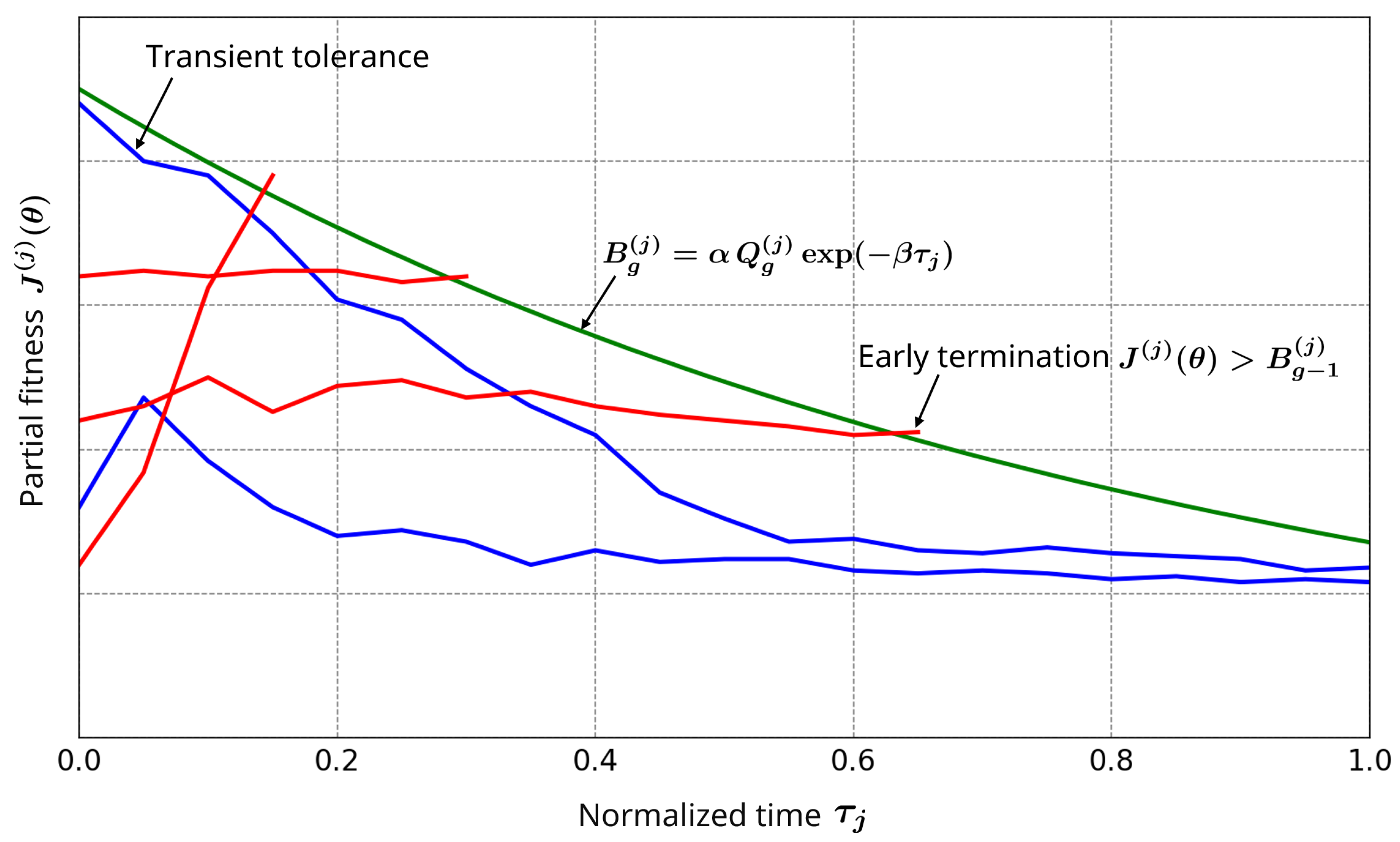
Figure 2.
Best fitness.
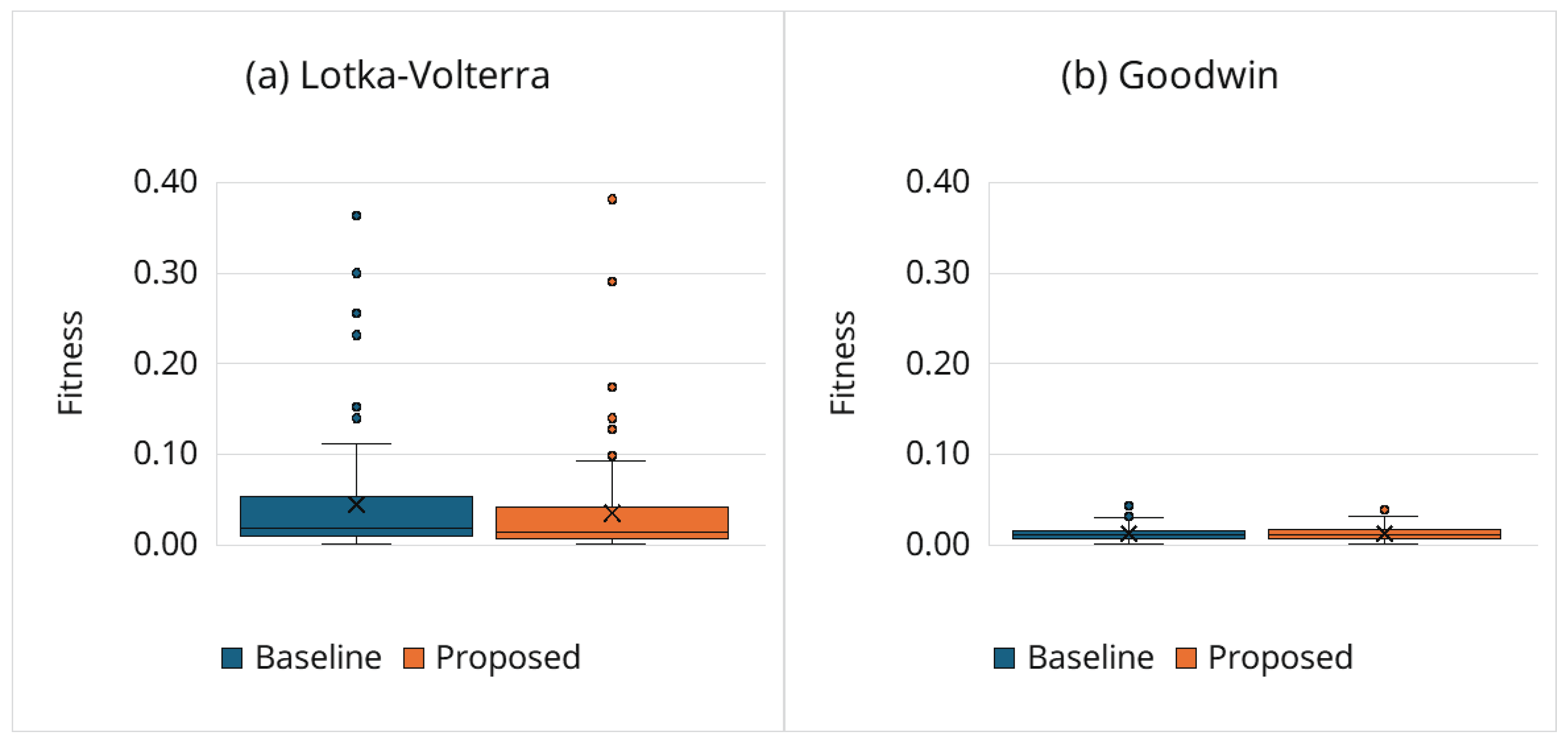
Figure 3.
Total RHS evaluations.
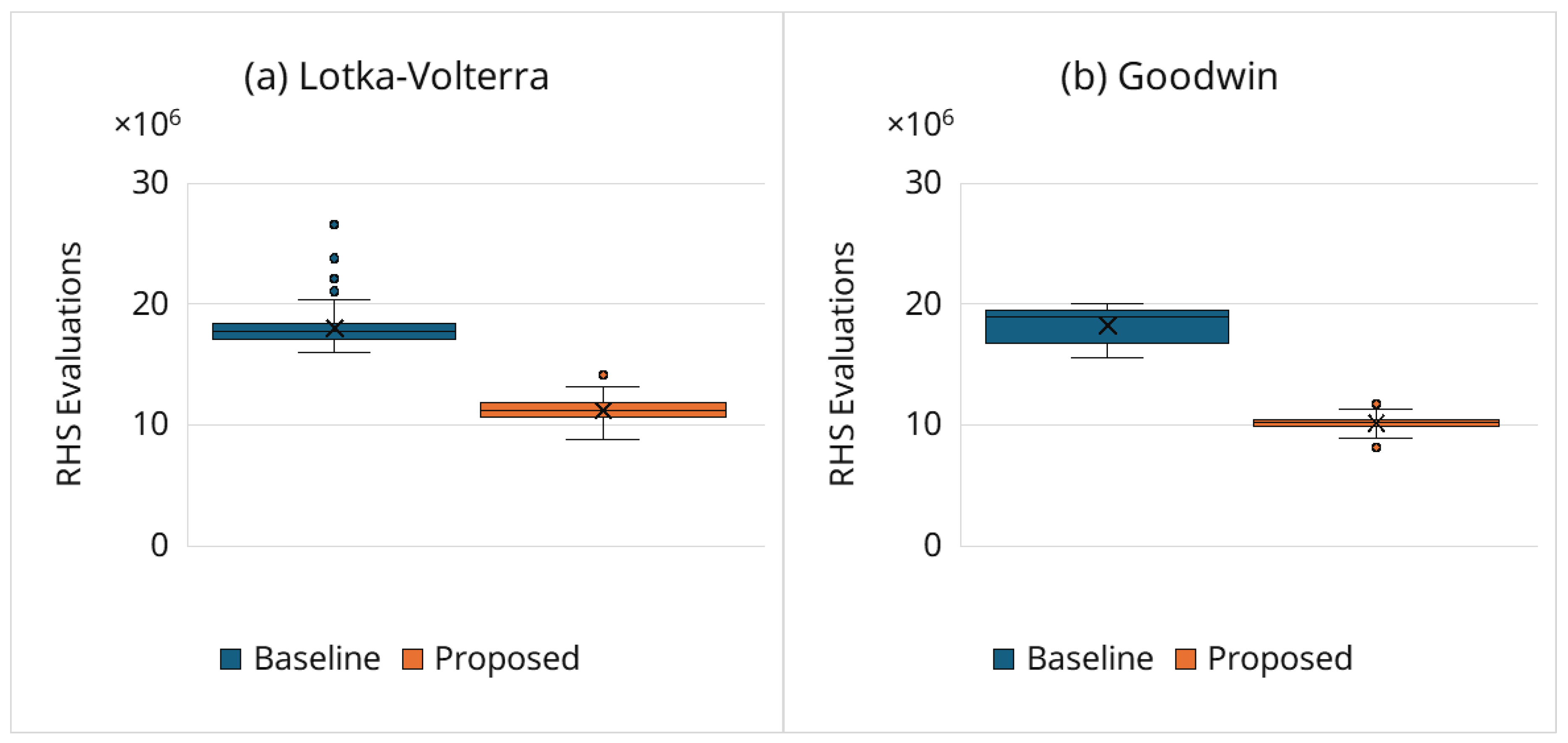
Figure 4.
Relative cost reduction (Equation (15)). The baseline is shown as a reference line at by definition.
Figure 4.
Relative cost reduction (Equation (15)). The baseline is shown as a reference line at by definition.

Figure 5.
Mean normalized termination index (Equation (16)). The baseline is shown as a reference line at by definition.
Figure 5.
Mean normalized termination index (Equation (16)). The baseline is shown as a reference line at by definition.
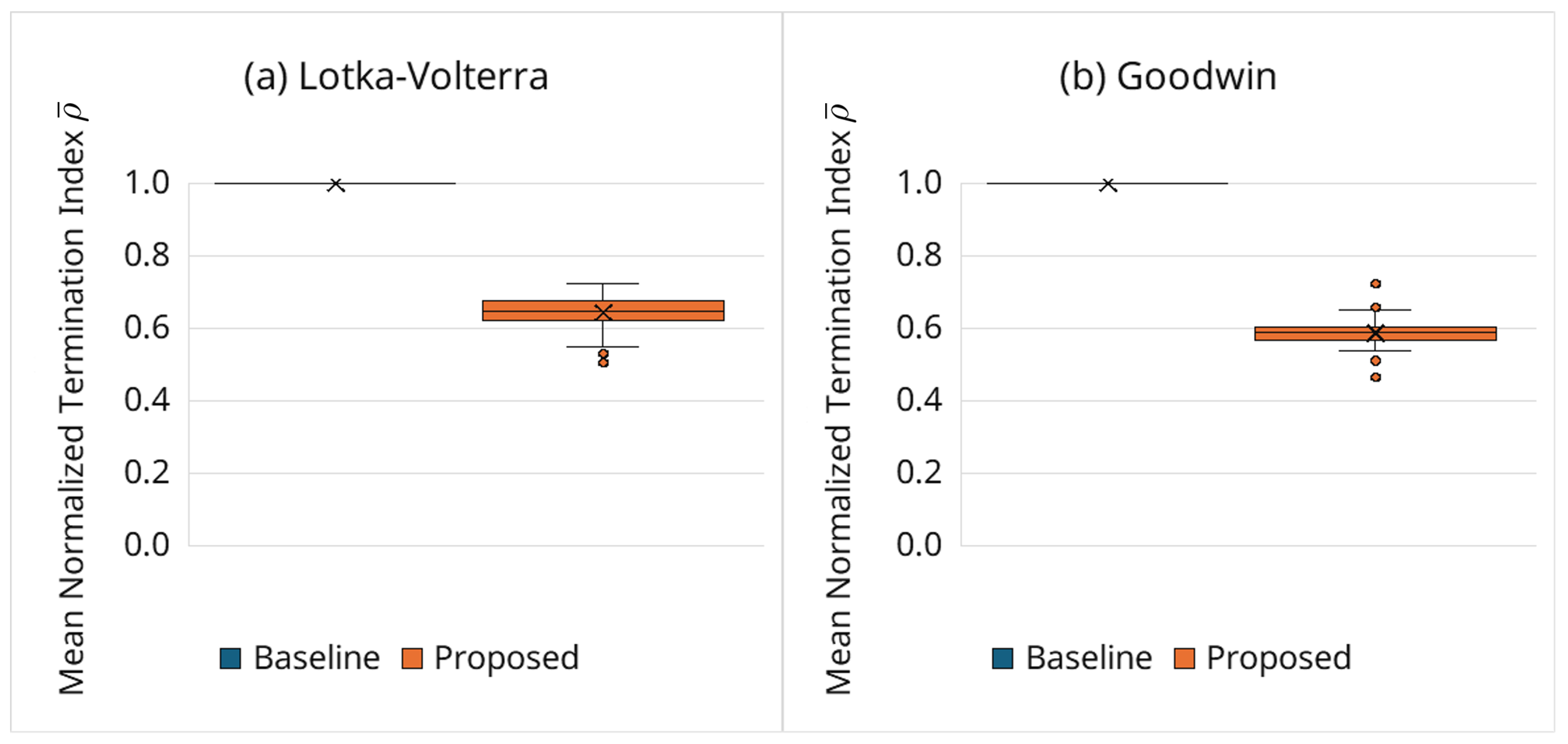
Figure 6.
Generation-wise evolution of (left) and the time-adaptive termination boundaries (right) as functions of the observation index j. Early indices are intentionally permissive, while later indices are stricter (Equation (10)). Across generations, the curves shift downward and stabilize, reflecting population-level improvement and threshold convergence. At small j, trajectories remain near the initial states, and relative errors are small, resulting in higher Q and B values that decrease as j increases. Curves overlay generations 25, 50, 75, 100.
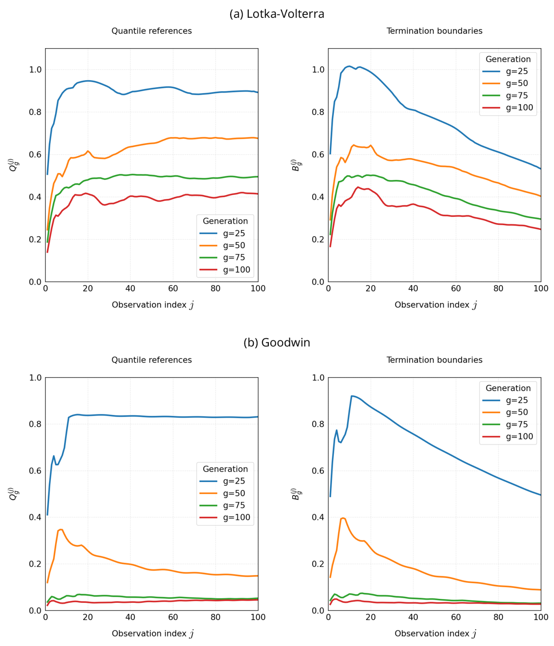
Figure 7.
Sensitivity of the proposed framework to .
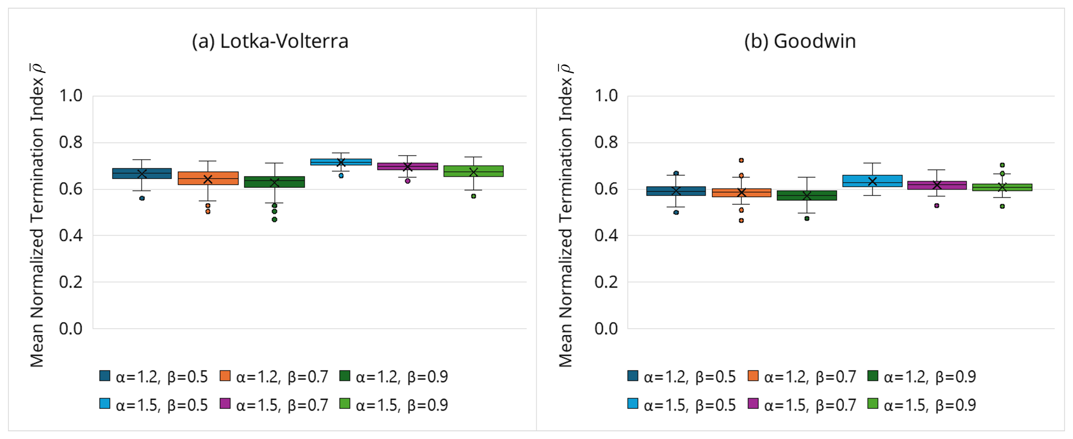
Figure 8.
Goodwin trajectories for at ; sustained, damped (gradual amplitude decay for ).
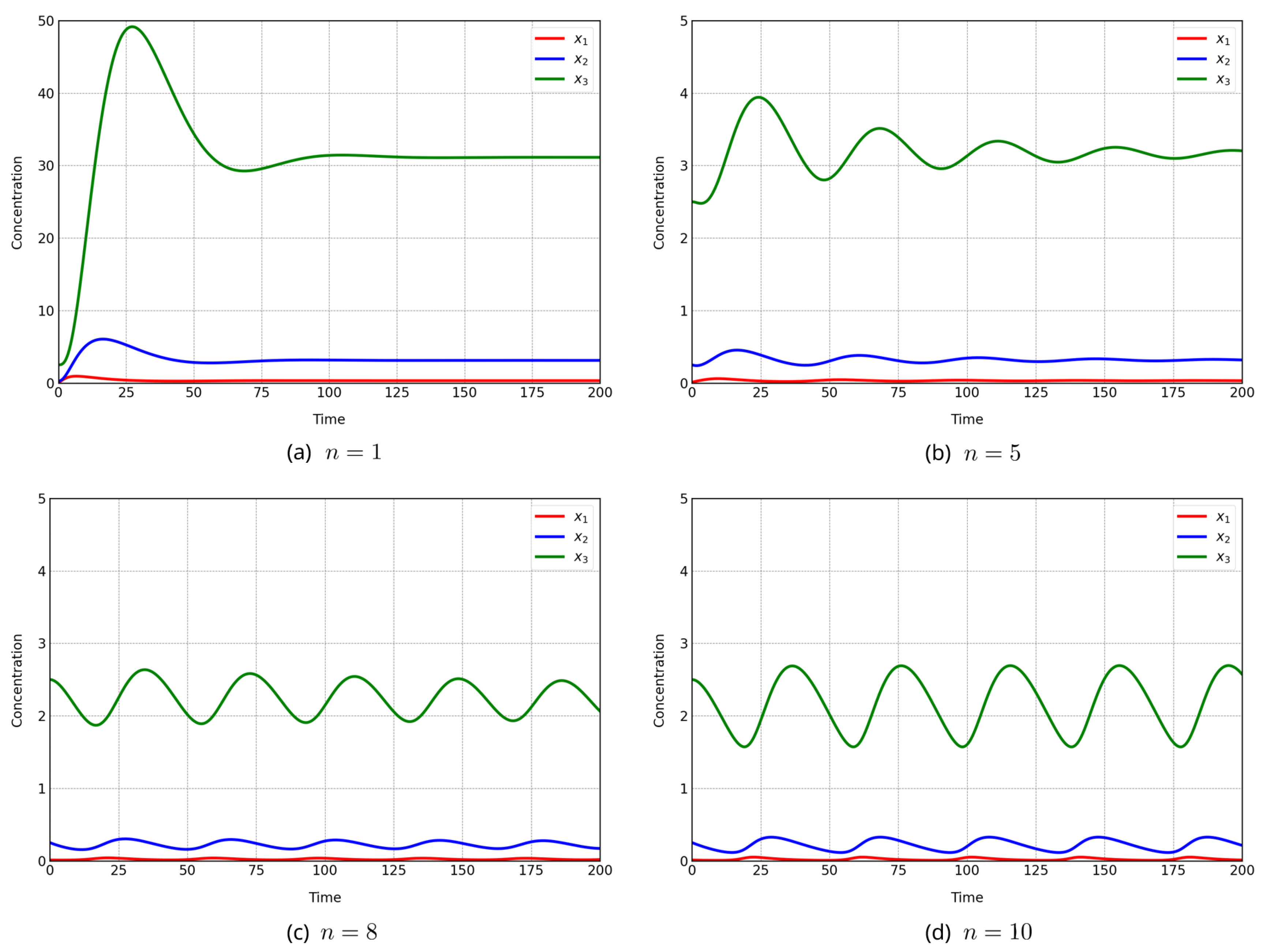
Figure 9.
(a) Early-termination rate vs. Hill coefficient n. (b) Mean among terminated candidates vs. n: early termination for ; later termination for and 8 (weakly damped trajectories).
Figure 9.
(a) Early-termination rate vs. Hill coefficient n. (b) Mean among terminated candidates vs. n: early termination for ; later termination for and 8 (weakly damped trajectories).
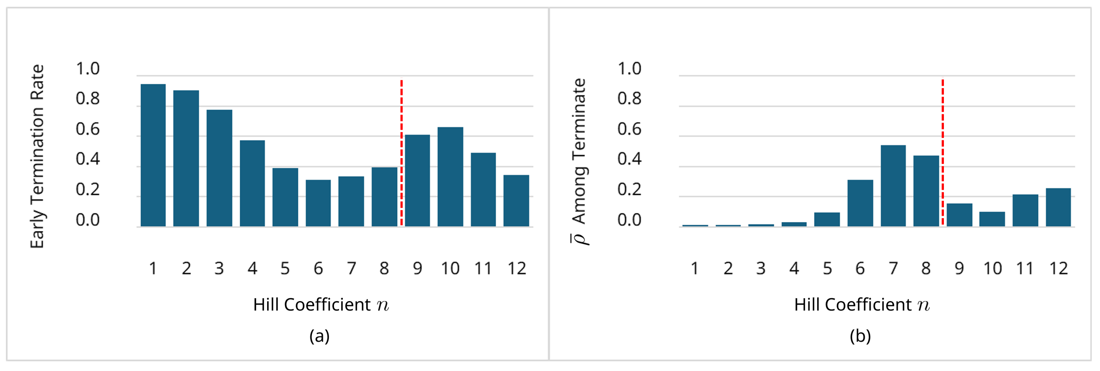

Table 1.
Trade-offs in reference update timing for simulation termination.
| Aspect | Early update | Delayed update |
|---|---|---|
| Computational efficiency | High | Moderate |
| Risk of false negatives | High | Low |
| Preservation of solution diversity | Low | High |
Table 2.
Experimental settings (GA/Powell method/Adaptive termination/Solver/Data).
| Category | Name | Symbol/Value | Notes |
|---|---|---|---|
| Genetic algorithm | Population size | Real-coded GA in log space (Equation (6)) | |
| Offspring | Generated via AREX | ||
| Parents | JGG partial replacement (Equation (7)) | ||
| Generations | Maximum generation | ||
| Parameter bounds | Kinetic parameter bounded relative to ground-truth | ||
| Powell method | Function | SciPy minimize | Maximum number of iterations is set to 200 |
| Starts | Initialized from top-ranked GA solutions | ||
| Termination boundary | Fixed (no updates during Powell) | ||
| Adaptive termination | Quantile level | For (Equation (9)) | |
| Tolerance factor | Controls the tolerance boundary (Equation (10)) | ||
| Decay rate | Controls time-dependent strictness (Equation (10)) | ||
| Warm-up | — | evaluated without adaptive termination | |
| Boundary lag | 1 generation | Evaluate at g using (Equation (11)) | |
| Reference retention rule | — | If no valid offspring: retain , (Equation (12)) | |
| Rejection penalty | For ranking; excluded from quantile computation | ||
| Objective | Stabilization constant | Treatment of zero/near-zero measurements (Equation (4)) | |
| Solver | Integrator | SciPy RK45 | Explicit Runge–Kutta; shared across frameworks |
| Tolerances | rtol , atol | Fixed across runs | |
| Maximum step | Equal to the sampling interval (Equation (17)) | ||
| Data | Sampling grid | 100 points over | Per condition; excludes |
| Observables (Lotka–Volterra) | Fully observed | ||
| Observables (Goodwin) | Partially observed (single variable) |
Table 3.
Trade-offs in reference update timing for simulation termination.
| Hill coefficient n | 1–6 | 7 | 8 | 9 | 10 | 11 | 12 |
|---|---|---|---|---|---|---|---|
| Baseline | 0 | 1 | 8 | 42 | 44 | 5 | 0 |
| Proposed | 0 | 0 | 4 | 42 | 45 | 9 | 0 |
Disclaimer/Publisher’s Note: The statements, opinions and data contained in all publications are solely those of the individual author(s) and contributor(s) and not of MDPI and/or the editor(s). MDPI and/or the editor(s) disclaim responsibility for any injury to people or property resulting from any ideas, methods, instructions or products referred to in the content. |
© 2026 by the authors. Licensee MDPI, Basel, Switzerland. This article is an open access article distributed under the terms and conditions of the Creative Commons Attribution (CC BY) license (http://creativecommons.org/licenses/by/4.0/).
Copyright: This open access article is published under a Creative Commons CC BY 4.0 license, which permit the free download, distribution, and reuse, provided that the author and preprint are cited in any reuse.


