Do Technical Indicators Improve Deep Learning Forecasts? An Empirical Ablation Study Across Asset Classes

1. Introduction

Financial time series forecasting poses fundamental challenges for machine learning—non-stationarity, low signal-to-noise ratios, complex temporal dependencies, and structural breaks driven by shifting market regimes [1,2]. Reliable price prediction underpins portfolio allocation, algorithmic trading, and risk management across global financial markets. Over the past decade, deep learning methods, particularly recurrent neural networks such as Long Short-Term Memory (LSTM) [3] and Gated Recurrent Units (GRU) [4], have become standard tools for capturing sequential dependencies in financial data [5].

A central and unresolved question in this domain concerns the role of handcrafted features—specifically, technical indicators. Technical analysis, which traces its origins to Charles Dow’s market theories in the late nineteenth century [6], holds that price patterns and derived momentum, trend, and volatility signals carry exploitable predictive information. Indicators such as the Relative Strength Index (RSI), Moving Average Convergence Divergence (MACD), and Bollinger Bands remain widely used in quantitative trading [7]. When these indicators are fed into deep learning models, however, a fundamental tension emerges: do they supply complementary information that genuinely improves predictions, or do deep neural networks already extract equivalent patterns from raw price data, rendering indicators redundant—or even harmful?

The existing literature offers conflicting answers. Several studies report improved accuracy when technical indicators augment deep learning inputs [8,9,10], while others find that raw Open-High-Low-Close-Volume (OHLCV) data yields equivalent or superior results [11,12,13]. This disagreement is compounded by considerable methodological heterogeneity: studies vary widely in asset coverage, time periods, indicator selection, preprocessing, and evaluation protocols [14], making systematic comparison difficult.

1.1. Motivation and Research Gap

Despite the considerable body of work on technical analysis and deep learning for financial forecasting, a critical gap remains: there is no systematic, multi-asset ablation study that rigorously quantifies the marginal contribution of different technical indicator categories under controlled experimental conditions. The existing literature suffers from several interrelated limitations. Most studies focus on single assets or narrow asset classes—typically U.S. equities or a particular market index—limiting the generalisability of their conclusions. Indicator selection tends to be ad hoc, without systematic comparison across indicator categories or against raw-data baselines. Many studies also lack statistical rigour, reporting single-run results without multiple random seeds, confidence intervals, or significance testing. Moreover, indicator types—momentum, trend, and volatility—are frequently conflated rather than evaluated independently, and evaluation metrics vary widely across studies, making direct comparison difficult.

Taken together, these shortcomings make it hard to determine whether technical indicators genuinely enhance deep learning forecasting or whether reported improvements reflect overfitting, publication bias, or asset-specific artefacts. The literature offers limited guidance on which indicator categories contribute most across different asset classes, whether their benefits vary with market characteristics such as volatility or trading regime, and whether combining multiple indicator categories yields complementary gains or introduces harmful redundancy.

1.2. Objectives and Scope

This paper addresses these gaps through a controlled empirical investigation designed for reproducibility and statistical validity. Our primary objective is to determine whether—and how—technical indicators affect deep learning-based next-day price prediction relative to a raw OHLCV baseline. We examine this question along three dimensions: (1) indicator categories, including momentum, trend, volatility, and their combinations; (2) asset classes, spanning commodities, cryptocurrencies, equities, foreign exchange, and market indices; and (3) recurrent architectures, comparing LSTM and GRU networks with equivalent capacity.

The study comprises 500 experiments across 10 assets, 5 feature configurations, 2 model architectures, and 5 random seeds per configuration. This factorial design enables us to isolate the marginal contribution of each indicator category, assess whether observed patterns are asset-specific or universal, and evaluate the potential for feature redundancy. All results are analysed using paired statistical tests with effect size measurements (Cohen’s d) to distinguish statistically significant differences from practically meaningful ones.

Based on prior literature and practitioner intuition, one might expect technical indicators to enhance model performance by providing additional predictive signal—particularly when matched to an asset’s characteristics, for instance volatility indicators improving forecasts for highly volatile assets. One might also expect that comprehensive indicator combinations would achieve superior performance through feature complementarity. Our experimental design allows systematic evaluation of both expectations.

1.3. Contributions

This work contributes to the literature on technical analysis and deep learning for financial forecasting in four ways:

• Multi-asset empirical evaluation. We present a controlled ablation study spanning five asset classes with distinct market microstructures, volatility profiles, and trading dynamics, enabling us to assess whether findings generalise beyond the single-asset benchmarks common in prior work.
• Statistical rigour. Our experimental design incorporates multiple random seeds, paired hypothesis tests, effect size quantification, and aggregated reporting with standard deviations—accounting for the stochastic variability inherent in neural network training and distinguishing reliable differences from noise.
• Indicator category decomposition. By evaluating momentum, trend, and volatility indicators both individually and in combination, we identify differential impacts across indicator families and provide evidence of redundancy when multiple indicator types are combined.
• Practical guidelines. The findings translate into actionable recommendations for practitioners on feature engineering, baseline selection, and architecture choice in deep learning-based trading systems.

The remainder of this paper is organised as follows. Section 2 reviews related work on financial time series modelling, deep learning for financial markets, and the integration of technical indicators with machine learning. Section 3 describes the dataset, asset selection, and preprocessing pipeline. Section 4 details the model architectures, training procedures, and evaluation metrics. Section 5 presents the experimental protocol and implementation details. Section 6 reports quantitative findings with statistical analysis. Section 7 interprets the results, discusses their implications and limitations, and outlines directions for future research. Section 8 summarises the principal contributions.

2. Related Work

This section organises the relevant literature into five thematic areas that contextualise the present study: the fundamental challenges of financial time series modelling (Section 2.1), deep learning for financial markets (Section 2.2), the integration of technical indicators with machine and deep learning models (Section 2.3), evaluation methodology and statistical practice in empirical research (Section 2.4), and the empirical studies most closely related to our own (Section 2.5).

2.1. Financial Time Series: Challenges and Properties

Financial time series exhibit well-documented statistical properties that set them apart from other sequential data and pose particular difficulties for predictive modelling. Cont [1] provides a canonical catalogue of these stylised facts, including heavy-tailed return distributions, volatility clustering (long memory in absolute returns), the near-absence of linear autocorrelation in raw returns, and leverage effects. These regularities are observed across asset classes and time scales, implying that forecasting models must accommodate non-Gaussian dynamics and time-varying second moments rather than relying on stationarity assumptions.

The Efficient Market Hypothesis (EMH), formalised by Fama [15], holds that asset prices fully reflect available information, implying that patterns derived from historical prices—the very foundation of technical analysis—cannot produce systematic predictive gains. In its weak form, the EMH directly challenges the premise that technical indicators computed from past prices carry exploitable signal. Early empirical evidence largely supported this view: Fama and Blume [16] found that filter-based trading rules failed to outperform buy-and-hold strategies once transaction costs were taken into account. Later work, however, identified contexts in which technical patterns appear profitable. Lo, Mamaysky, and Wang [17] used nonparametric kernel regression to detect chart patterns on NASDAQ stocks and found statistically significant incremental information content. Brock, Lakonishok, and LeBaron [18] showed that simple moving-average and trading-range breakout rules generated excess returns on the Dow Jones Industrial Average, although concerns about data snooping and survivorship bias persist. Neely, Weller, and Dittmar [19] reported profitability of technical trading rules in foreign exchange markets using genetic programming, suggesting that currency markets may be particularly receptive to technical strategies.

Lo [20] proposes the Adaptive Markets Hypothesis (AMH) as a reconciliation of market efficiency with episodic predictability. Under the AMH, the profitability of technical patterns fluctuates over time as market participants adapt, providing a theoretical rationale for why indicator utility might differ across assets, time periods, and market regimes. This framework motivates our multi-asset, multi-period experimental design and underscores the need to test indicator utility across diverse market conditions rather than on a single benchmark.

Tsay [21] offers a comprehensive treatment of the econometric challenges inherent in financial time series, including non-stationarity, structural breaks, and conditional heteroscedasticity. These properties motivate the use of flexible nonlinear models such as deep neural networks, but they also raise concerns about feature engineering choices that presuppose fixed distributional characteristics—precisely the kind of assumptions embedded in many conventional technical indicators with fixed lookback windows and static parameters.

2.2. Deep Learning for Financial Markets

Deep learning methods have been applied with growing frequency to financial forecasting, driven by their ability to approximate nonlinear relationships without requiring explicit feature specification [22]. Sezer, Gudelek, and Ozbayoglu [2] survey more than 150 studies published between 2005 and 2019, documenting the progressive shift from traditional econometric models toward neural architectures and identifying recurrent networks as the most widely adopted family for sequential financial data.

Recurrent architectures.

Long Short-Term Memory (LSTM) networks [3] remain the dominant recurrent architecture in financial applications. Their gating mechanism—comprising input, forget, and output gates—enables selective retention of information across time steps, thereby addressing the vanishing gradient problem that hampers standard recurrent networks. Fischer and Krauss [5] showed that LSTM networks outperformed random forests, logistic regression, and standard feedforward networks for daily return prediction on S&P 500 constituents over a 25-year period, providing one of the most extensive evaluations of LSTM in a financial setting to date.

Gated Recurrent Units (GRU) [4] offer a computationally lighter alternative by merging the cell state and hidden state into a single mechanism governed by update and reset gates. Empirical comparisons across sequence modelling tasks have generally found GRU performance on par with LSTM, with neither architecture consistently dominating [23,24]. This approximate parity motivates our controlled comparison under matched hyperparameters to examine whether architectural differences interact with feature configuration choices.

Multi-asset and large-scale studies.

Gu, Kelly, and Xiu [25] conducted a landmark study comparing machine learning methods—including deep neural networks, random forests, and gradient-boosted trees—for cross-sectional asset pricing using 94 firm-level characteristics. Neural networks achieved the highest out-of-sample $R^2$ for monthly return prediction, establishing an important methodological lesson: large-scale, multi-asset evaluation with proper statistical assessment is essential for drawing reliable conclusions in financial machine learning.

Krauss, Do, and Huck [26] applied deep neural networks, gradient-boosted trees, and random forests to statistical arbitrage on the S&P 500, finding that deep networks achieved the highest mean daily returns but exhibited substantial variability across sub-periods. Their analysis highlights how sensitive financial deep learning results can be to the evaluation window, reinforcing the need for robust multi-seed assessment—a principle that is central to our experimental design.

Sirignano and Cont [27] trained deep learning models on limit order book data from nearly 1,000 U.S. stocks simultaneously and found evidence for universal price formation features—statistical regularities that persist across individual assets. Their work supports the hypothesis that deep neural networks can discover latent representations directly from raw market data, potentially rendering handcrafted technical features redundant.

Surveys and open questions.

Lim and Zohren [28] survey deep learning for time-series forecasting, covering convolutional, recurrent, and attention-based architectures. They identify automatic feature learning as a key advantage of deep approaches over classical methods, but note that the empirical benefit of handcrafted features remains unresolved, particularly in financial domains where abundant domain knowledge tempts practitioners to over-engineer input representations. This open question motivates the controlled ablation study we present here.

2.3. Technical Indicators in Machine Learning and Deep Learning Models

The use of technical indicators as input features for machine learning and deep learning models has generated a substantial body of work, yet conclusions about their predictive value remain inconsistent. This inconsistency can be traced to differences in asset coverage, indicator selection, model architectures, preprocessing pipelines, and evaluation protocols.

Classical machine learning with indicators.

Kara, Boyacioglu, and Baykan [29] compared artificial neural networks (ANNs) and support vector machines (SVMs) for predicting the direction of the Istanbul Stock Exchange index using ten technical indicators. Both models achieved directional accuracies exceeding 70%, with ANNs performing slightly better. Crucially, however, the study did not include a raw-price baseline, so it is not possible to isolate the indicators’ contribution from the model’s own capacity.

Patel et al. [30] partially addressed this limitation by comparing two input representations—raw technical indicator values versus trend-deterministic binary encodings of indicator signals—for stock and index prediction using ANNs, SVMs, random forests, and naïve Bayes classifiers across several Indian equities and indices. They found that the trend-deterministic representation improved accuracy for all models, demonstrating that how indicators are encoded can matter as much as which indicators are selected. Although their study spans multiple assets, it employs classical ML rather than deep learning.

Zhong and Enke [31] systematically evaluated dimensionality reduction methods (PCA, kernel PCA, fuzzy robust PCA) applied to 60 technical indicator features for daily S&P 500 return forecasting with ANNs. They found that principal component analysis improved prediction accuracy, suggesting that while raw indicator sets contain useful information, their high dimensionality and multicollinearity introduce noise that benefits from reduction—an observation directly relevant to the feature redundancy we document in the present study.

Deep learning with indicators.

Bao, Yue, and Rao [8] proposed a multi-stage pipeline combining wavelet transforms for denoising, stacked autoencoders for feature learning, and LSTM for prediction, incorporating technical indicators alongside transformed price data. Although their architecture improved upon several baselines on six stock indices, the denoising and autoencoder stages confound assessment of raw indicator contributions, and the absence of a pure OHLCV baseline makes it impossible to attribute gains specifically to the indicators.

Selvin et al. [10] compared CNN, standard RNN, and LSTM architectures using sliding windows of OHLCV and indicator features for Indian stock prediction. They observed modest improvements with indicators for certain asset–architecture combinations, but the gains were not uniform across stocks—foreshadowing the asset-specific heterogeneity that our study documents more systematically.

Nelson, Pereira, and de Oliveira [9] applied LSTM networks with 180 technical indicator features to Brazilian equity prediction, reporting a directional accuracy of roughly 55.9% on Ibovespa constituents. While demonstrating that LSTM can process high-dimensional indicator sets, their study again lacks a raw-price baseline, precluding attribution of performance to indicator content rather than model capacity.

Chong, Han, and Park [11] investigated deep feedforward networks with both raw returns and technical indicator features for Korean equity prediction. Notably, models trained on raw residual data performed comparably to those using covariance-stationary indicator features, offering early evidence that deep networks can learn equivalent representations without explicit feature engineering. This finding is particularly germane to the present work, as it motivates our hypothesis that recurrent networks may render technical indicators redundant.

Hoseinzade and Haratizadeh [32] proposed CNNpred, a CNN-based framework that combines technical indicators, macroeconomic variables, and cross-market features for S&P 500 prediction. While achieving competitive accuracy, they observed diminishing marginal returns from additional feature categories—consistent with our finding that comprehensive indicator sets can degrade performance through redundancy and noise.

Synthesis.

Across these studies, a pattern emerges: indicator benefits are most frequently reported in settings that use classical ML models with limited feature-learning capacity, focus on single markets, and lack rigorous raw-data baseline comparisons. Studies employing deeper architectures or including raw-data baselines more often report null or mixed effects. This asymmetry motivates a systematic ablation that controls for model architecture and evaluates distinct indicator categories against an OHLCV baseline across diverse asset classes.

2.4. Evaluation Methodology, Ablation Studies, and Statistical Practice

Sound evaluation methodology is critical for drawing reliable conclusions from machine learning experiments, yet methodological shortcomings remain common in applied financial ML research.

Dietterich [33] demonstrated that single-run comparisons between learning algorithms are statistically unreliable, showing that commonly used tests can exhibit inflated Type I error rates when applied to a single train–test split. He recommended multiple random initialisations when comparing trained models and approximate randomisation tests for algorithm-level comparisons. Our multi-seed protocol with paired statistical testing follows this principle, accounting for the stochastic variability inherent in neural network training—variability that is routinely ignored in financial deep learning studies where results from a single run are reported without any uncertainty quantification.

Henderson et al. [34] documented alarming variability in deep reinforcement learning results, showing that reported improvements frequently fall within the noise introduced by random seeds, hyperparameter choices, and implementation details. They advocate reporting results over multiple seeds with confidence intervals, significance tests, and ablation studies—practices that remain uncommon in financial deep learning yet are indispensable for separating genuine effects from training artefacts. Our factorial experimental design and multi-seed protocol directly implement their recommendations.

Makridakis, Spiliotis, and Assimakopoulos [35] compared statistical and machine learning forecasting methods across 1,045 monthly time series from the M3 competition, finding that simple statistical methods (exponential smoothing, ARIMA) frequently outperformed more complex ML models when evaluation was conducted rigorously with proper out-of-sample testing. Their findings underscore the value of strong baselines and caution against the assumption that greater model or feature complexity translates to better predictions—a caution directly relevant to our question of whether indicator-enriched inputs outperform parsimonious OHLCV representations.

2.5. Closest Related Empirical Studies

Several prior studies address questions that overlap with the present work, though none combine multi-asset coverage, controlled indicator-category ablation, and rigorous multi-seed statistical evaluation in the way our design does.

Nti, Adekoya, and Weyori [14] carried out a systematic review of 122 studies on stock market prediction using fundamental and technical analysis. They document substantial heterogeneity in data sources, feature sets, models, and evaluation protocols, and identify the absence of standardised benchmarks and the dominance of single-asset, single-run evaluations as major obstacles to cumulative knowledge building. Our factorial design across ten assets, five feature configurations, two architectures, and five random seeds addresses these shortcomings directly.

Chong, Han, and Park [11] provide the closest methodological precedent: they compared raw versus indicator-augmented inputs for deep learning and found comparable performance on Korean equities. Their analysis, however, is limited to a single market and a feedforward architecture. We extend their approach to recurrent architectures across five distinct asset classes, enabling an assessment of cross-market generalisability.

Tsai and Hsiao [36] proposed combining multiple feature selection methods (union, intersection, multi-intersection) for stock prediction and showed that carefully curated feature subsets outperform both complete feature sets and individual selection approaches. Their observation that feature subsets frequently outperform the full set parallels our finding that the all-indicators configuration (E4) yields the worst performance, although their work is situated in classical ML rather than deep learning.

Cao, Li, and Li [12] combined signal decomposition (CEEMDAN) with LSTM for financial time series forecasting and found that preprocessing raw data through decomposition improved accuracy relative to direct LSTM application. Their approach suggests that transforming the temporal structure of inputs may be more effective than appending handcrafted indicator features—an alternative paradigm for feature enrichment that is consistent with our finding that explicit indicators can be redundant for deep recurrent networks.

Kim and Kim [37] developed a feature-fusion LSTM-CNN architecture using multiple representations of the same underlying price data, including technical indicators and candlestick image encodings. They observed performance saturation when combining redundant representations, paralleling our finding that the comprehensive all-indicators configuration performs worse than any single-category variant because of accumulated feature redundancy.

Summary of the research gap.

The reviewed literature reveals a clear gap: no prior study has conducted a controlled, multi-asset ablation examining the marginal contribution of categorised technical indicator groups—momentum, trend, and volatility—against a raw OHLCV baseline, using recurrent deep learning architectures with statistically rigorous multi-seed evaluation and formal significance testing. The present study fills this gap through a factorial experimental design spanning five asset classes, two recurrent architectures, and 500 total experiments.

3. Data

This section describes the assets, data sources, preprocessing pipeline, and technical indicator specifications used in our experiments. We emphasise reproducibility, causal feature construction, and the prevention of look-ahead bias.

3.1. Asset Selection

To evaluate forecasting performance under diverse market conditions, we select 10 assets from five asset classes. All time series consist of daily OHLCV (Open, High, Low, Close, Volume) data obtained from Yahoo Finance. Table 1 provides summary statistics, including approximate date ranges and sample counts.

Commodities.

• Crude Oil (WTI Futures). West Texas Intermediate crude oil, a benchmark for global oil prices, exhibiting high volatility and sensitivity to geopolitical events. Daily data from 2010-01-04 to 2025-12-31 (4,024 trading days).
• Gold (XAU/USD). Spot gold price in U.S. dollars, traditionally considered a safe-haven asset with moderate volatility. Daily data from 2010-01-04 to 2025-12-31 (4,023 trading days).

Cryptocurrencies.

• Bitcoin (BTC/USD). The largest cryptocurrency by market capitalisation, characterised by extreme volatility and 24/7 trading. Daily data from 2014-09-17 to 2025-12-31 (4,124 trading days).
• Ethereum (ETH/USD). The second-largest cryptocurrency, serving as the foundation for decentralised applications. Daily data from 2017-11-09 to 2025-12-31 (2,975 trading days).

Equities.

• Apple Inc. (AAPL). A large-cap technology stock with moderate volatility and high liquidity. Daily data from 2010-01-04 to 2025-12-31 (4,024 trading days).
• Microsoft Corporation (MSFT). A large-cap technology stock with similar characteristics to AAPL. Daily data from 2010-01-04 to 2025-12-31 (4,024 trading days).

Foreign exchange.

• EUR/USD. The most actively traded currency pair globally, exhibiting lower volatility than equities and commodities. Daily data from 2010-01-01 to 2025-12-31 (4,165 trading days).
• USD/JPY. A major currency pair reflecting U.S.–Japan monetary policy dynamics. Daily data from 2010-01-01 to 2025-12-31 (4,165 trading days).

Market indices.

• NASDAQ Composite. A technology-weighted U.S. equity index tracking over 3,000 stocks. Daily data from 2010-01-04 to 2025-12-31 (4,024 trading days).
• S&P 500. A capitalisation-weighted index of 500 large U.S. companies, widely used as a benchmark. Daily data from 2010-01-04 to 2025-12-31 (4,024 trading days).

3.2. Data Format and Source

All datasets consist of daily OHLCV records downloaded from Yahoo Finance via the yfinance Python library. Each record contains:

• Date: Trading date in UTC.
• Open: Opening price for the trading session.
• High: Highest intraday price.
• Low: Lowest intraday price.
• Close: Closing price (adjusted for splits where applicable).
• Volume: Number of shares or contracts traded.

The prediction target is the raw closing price one trading day ahead. Input features are normalised prior to model training (see Section 4); the target, however, remains in its original units to keep error metrics directly interpretable.

3.3. Feature Configurations

We evaluate five feature configurations (E0–E4) in our ablation study. Technical indicator parameters follow widely used defaults (consistent with libraries such as TA-Lib) to facilitate comparability with prior work.

E0: OHLCV only (baseline).

The baseline configuration includes the five raw price and volume series: Open, High, Low, Close, and Volume. This serves as the control condition against which all indicator-augmented configurations are compared.

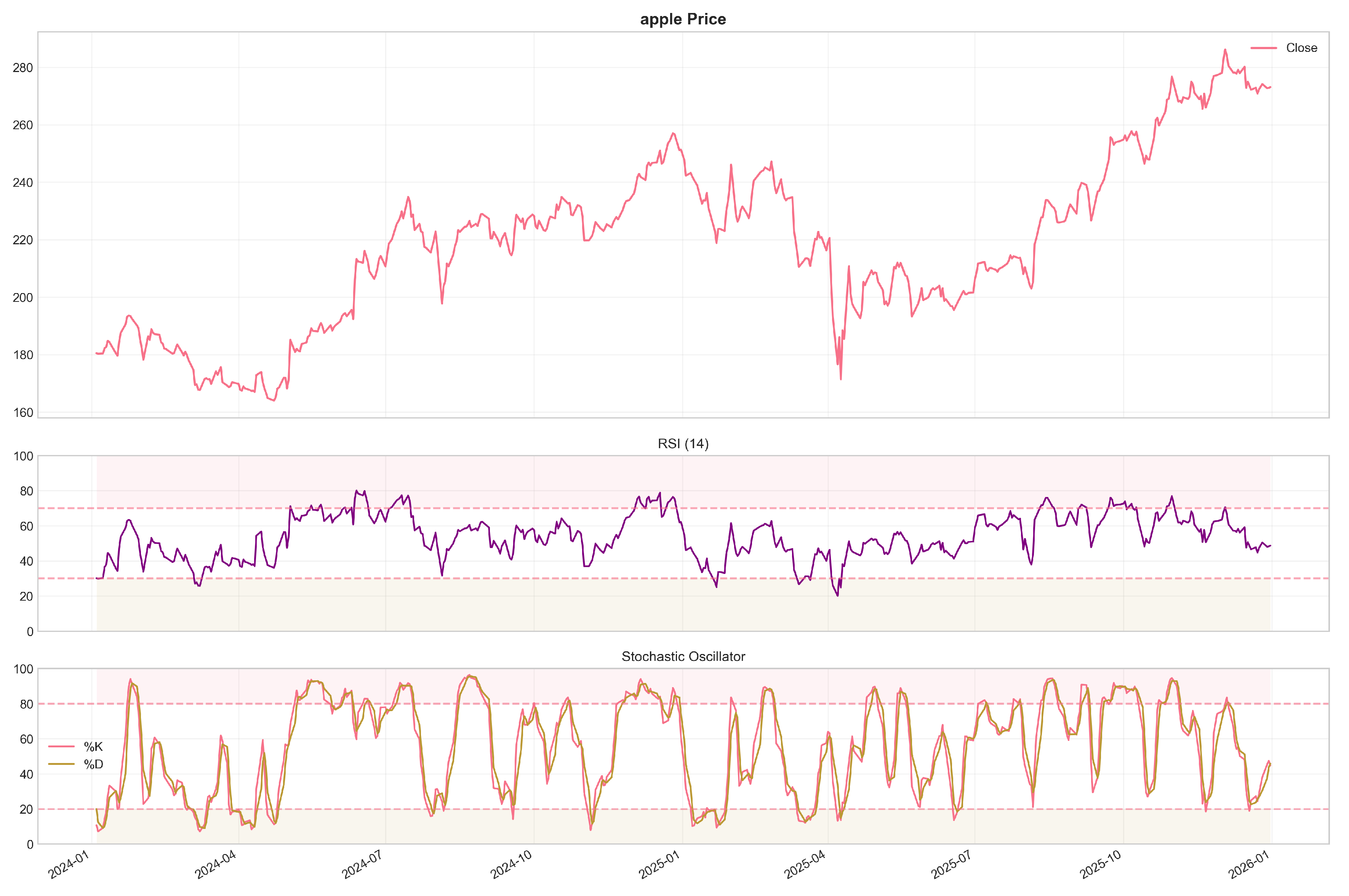
E1: OHLCV + momentum indicators.

Baseline features augmented with three momentum oscillators:

• Relative Strength Index (RSI, 14-period)
• Stochastic %K (14-period high/low window, 3-period smoothing)
• Stochastic %D (3-period SMA of %K)

Total features: 8

Figure 1. Momentum indicators computed for a representative asset over a sample period. The Relative Strength Index (RSI, top panel) oscillates between 0 and 100, with values above 70 indicating overbought conditions and values below 30 indicating oversold conditions. Stochastic oscillators (%K and %D, bottom panel) similarly range from 0 to 100 and are commonly used to detect momentum shifts and potential trend reversals.

Figure 1. Momentum indicators computed for a representative asset over a sample period. The Relative Strength Index (RSI, top panel) oscillates between 0 and 100, with values above 70 indicating overbought conditions and values below 30 indicating oversold conditions. Stochastic oscillators (%K and %D, bottom panel) similarly range from 0 to 100 and are commonly used to detect momentum shifts and potential trend reversals.

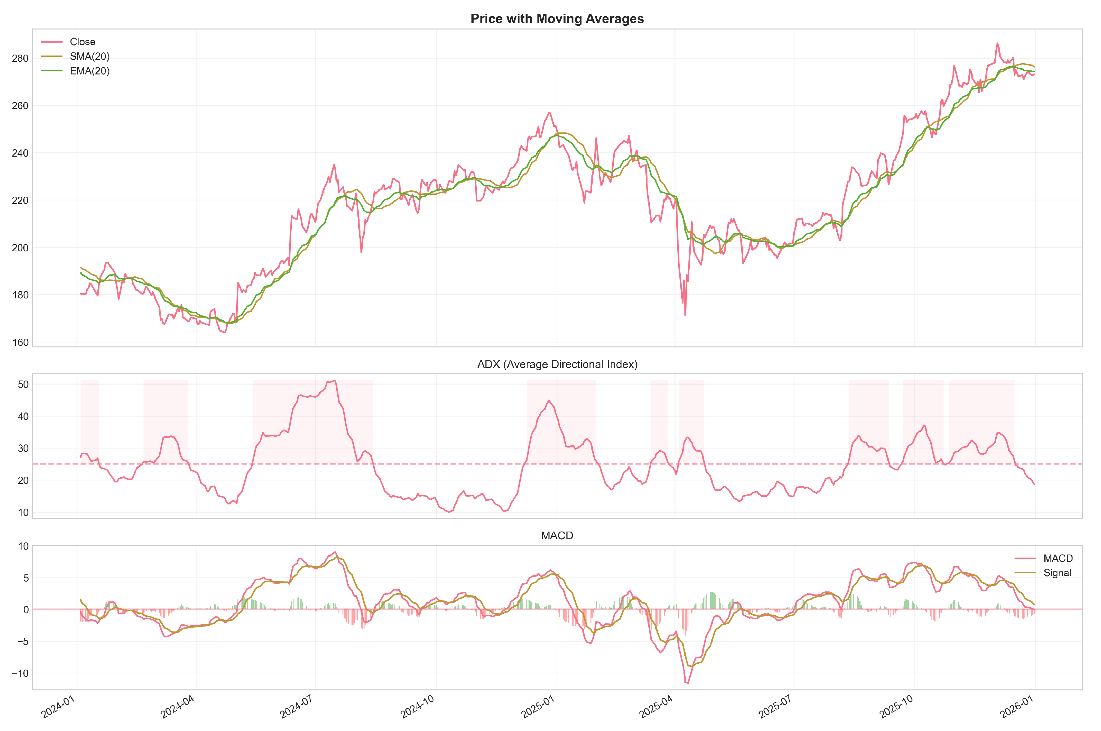
E2: OHLCV + trend indicators.

Baseline features augmented with six trend-following indicators:

• Simple Moving Average (SMA, 20-period)
• Exponential Moving Average (EMA, 20-period)
• Average Directional Index (ADX, 14-period)
• MACD line (12-period EMA − 26-period EMA)
• MACD signal line (9-period EMA of MACD)
• MACD histogram (MACD − signal)

Total features: 11

Figure 2. Trend indicators computed for a representative asset. Moving averages (SMA: Simple Moving Average; EMA: Exponential Moving Average) smooth price action to reveal underlying directional trends. The Average Directional Index (ADX) quantifies trend strength on a 0–100 scale regardless of direction, with values above 25 indicating a strong trend. MACD (Moving Average Convergence Divergence) components capture momentum shifts through moving average crossovers; the histogram shows the difference between the MACD line and its signal line.

Figure 2. Trend indicators computed for a representative asset. Moving averages (SMA: Simple Moving Average; EMA: Exponential Moving Average) smooth price action to reveal underlying directional trends. The Average Directional Index (ADX) quantifies trend strength on a 0–100 scale regardless of direction, with values above 25 indicating a strong trend. MACD (Moving Average Convergence Divergence) components capture momentum shifts through moving average crossovers; the histogram shows the difference between the MACD line and its signal line.

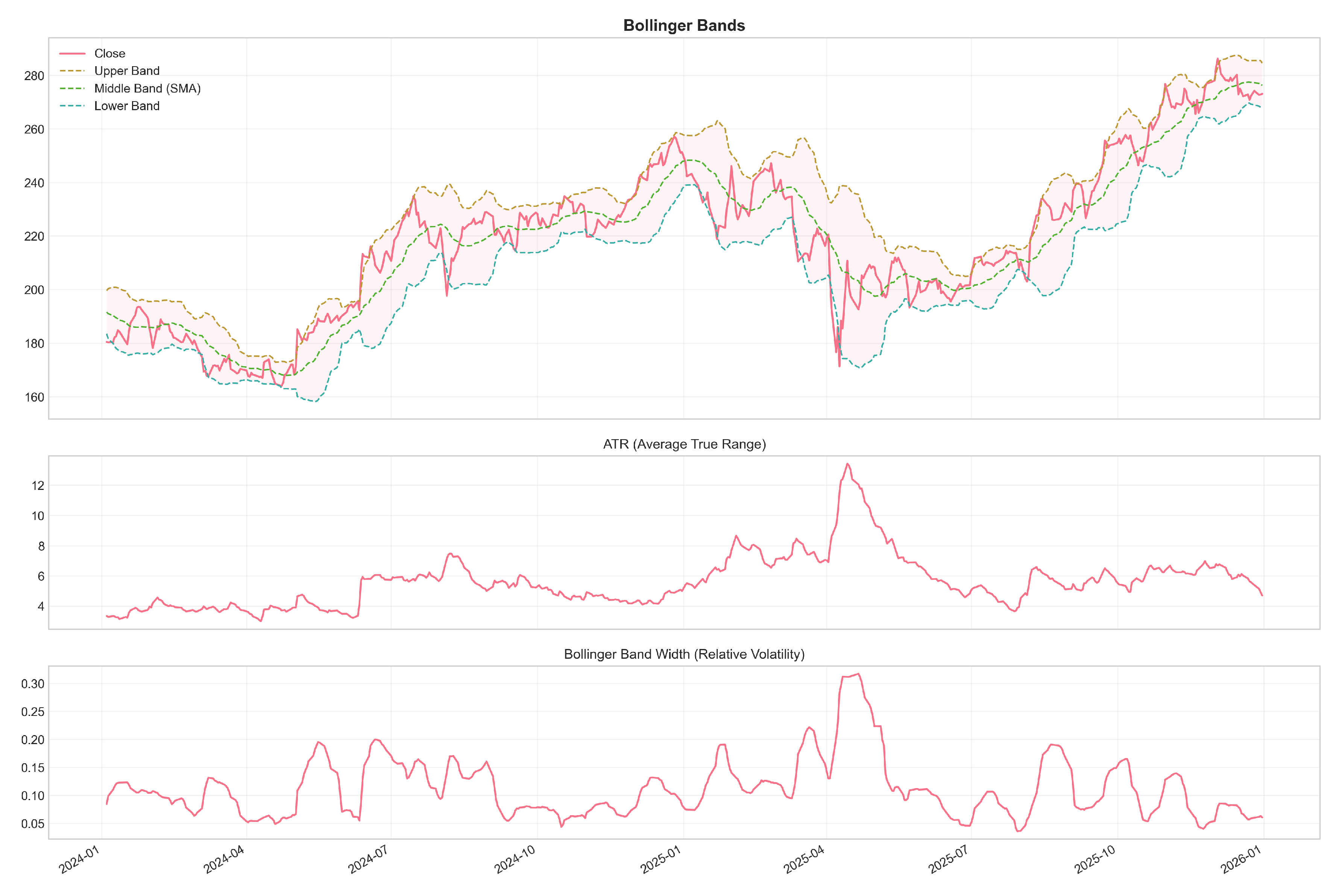
E3: OHLCV + volatility indicators.

Baseline features augmented with four volatility measures:

• Average True Range (ATR, 14-period)
• Bollinger Band upper boundary (20-period SMA $+2\sigma$)
• Bollinger Band lower boundary (20-period SMA $-2\sigma$)
• Bollinger %B (price position relative to bands, scaled 0–1)

Total features: 9

E4: OHLCV + all indicators.

A comprehensive configuration combining all indicators from E1, E2, and E3 with the baseline OHLCV features. Total features: 18

3.4. Technical Indicator Calculations

Indicators are computed using causal rolling or exponential filters (each indicator value depends only on current and past data). Implementations follow standard formulas; brief definitions are provided for completeness.

Relative Strength Index (RSI).

$$\mathrm{RSI}=100-{\displaystyle \frac{100}{1+\mathrm{RS}}}$$

(1)

where RS is the ratio of the exponentially weighted average of gains to losses over the lookback period (14 by default).

Figure 3. Volatility indicators computed for a representative asset. Average True Range (ATR, top panel) measures the average magnitude of price movements over the lookback period, capturing market volatility independent of direction. Bollinger Bands (middle panel) construct dynamic price channels around a 20-period moving average using $\pm 2$ standard deviations; bands widen during volatile periods and contract during calm markets. The %B indicator (bottom panel) shows the position of the current price within the bands, scaled from 0 (at lower band) to 1 (at upper band).

Figure 3. Volatility indicators computed for a representative asset. Average True Range (ATR, top panel) measures the average magnitude of price movements over the lookback period, capturing market volatility independent of direction. Bollinger Bands (middle panel) construct dynamic price channels around a 20-period moving average using $\pm 2$ standard deviations; bands widen during volatile periods and contract during calm markets. The %B indicator (bottom panel) shows the position of the current price within the bands, scaled from 0 (at lower band) to 1 (at upper band).

Stochastic Oscillator.

$$\%K={\displaystyle \frac{C-L_n}{H_n-L_n}}\times 100$$

(2)

where C is the current close and $L_n$, $H_n$ are the lowest and highest prices over the previous n periods (we use $n=14$ and 3-period smoothing).

Moving Average Convergence Divergence (MACD).

$$\mathrm{MACD}={\mathrm{EMA}}_{12}-{\mathrm{EMA}}_{26}$$

(3)

The MACD signal is the 9-period EMA of the MACD line; the histogram is the MACD minus its signal.

Average True Range (ATR).

$$\mathrm{TR}=max(H-L,|H-C_{\mathrm{prev}}|,|L-C_{\mathrm{prev}}\left|\right)$$

(4)

$$\mathrm{ATR}=\mathrm{SMA}(\mathrm{TR},n)$$

(5)

We use a 14-period window for ATR.

Bollinger Bands.

$$\mathrm{Upper}\mathrm{Band}={\mathrm{SMA}}_{20}+2\sigma ,\mathrm{Lower}\mathrm{Band}={\mathrm{SMA}}_{20}-2\sigma$$

(6)

where $\sigma$ is the 20-period standard deviation of the closing price.

3.5. Feature Analysis

To understand the relationships among technical indicators and assess their potential for providing complementary information, we analyse the correlation structure of the full feature set. Figure 4 presents the Pearson correlation matrix for the comprehensive feature set (E4 configuration) computed on a representative asset (Apple Inc.).

Figure 4. Pearson correlation heatmap for the comprehensive indicator set (E4 configuration) applied to Apple Inc. Features are grouped by category: OHLCV, momentum, trend, and volatility. Darker shading indicates stronger correlations, revealing substantial multicollinearity within indicator categories.

Figure 4. Pearson correlation heatmap for the comprehensive indicator set (E4 configuration) applied to Apple Inc. Features are grouped by category: OHLCV, momentum, trend, and volatility. Darker shading indicates stronger correlations, revealing substantial multicollinearity within indicator categories.

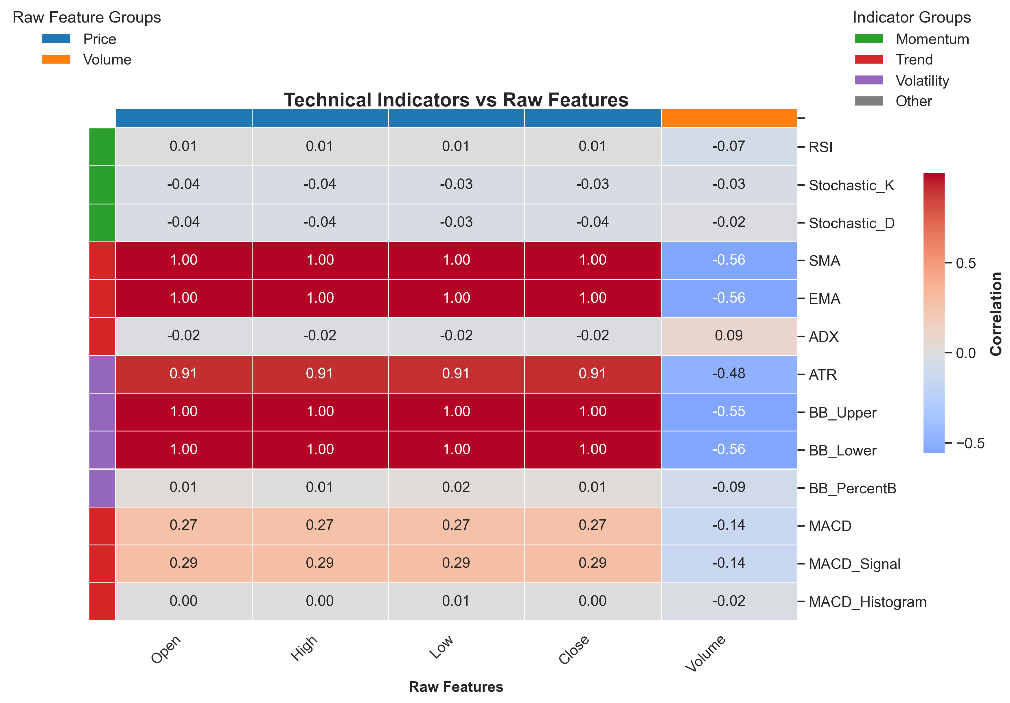
Several patterns stand out:

• Strong intra-category correlations: Indicators within the same family are highly correlated (e.g., SMA and EMA: $r=0.98$; MACD components: $r>0.90$).
• OHLCV relationships: Raw price features correlate moderately with trend indicators but less so with momentum and volatility measures.
• Momentum–volatility linkage: RSI and Stochastic oscillators show moderate correlation with Bollinger Band position ($r\approx 0.60$), reflecting their shared sensitivity to recent price extremes.
• Limited inter-category independence: Most cross-category correlation coefficients fall below 0.50, suggesting that different indicator families do capture distinct aspects of market dynamics.

This analysis informs the experimental design by highlighting the potential for redundancy, which may contribute to the performance degradation observed when all indicators are combined.

3.6. Problem Formulation

We formulate the task as supervised one-step-ahead forecasting of the raw closing price. Given a lookback window of length L with F features, each input is a matrix $X_{t-L+1:t}\in {\mathbb{R}}^{L\times F}$ and the target is the next-day close $y_{t+1}=C_{t+1}$. Models learn a mapping

$$f_{\theta }:{\mathbb{R}}^{L\times F}\to \mathbb{R},{\widehat{y}}_{t+1}=f_{\theta }\left(X_{t-L+1:t}\right).$$

(7)

Training minimises a regression loss (mean squared error, MSE, by default). We report multiple metrics on hold-out data including MSE, mean absolute error (MAE), and directional accuracy (sign of returns) to capture both magnitude and directional performance.

Primary forecasting horizon is one trading day ($h=1$). Sliding windows with stride 1 produce the supervised dataset used for training and evaluation; all window construction and indicator computation are causal to avoid leakage (see Section 3.10).

3.7. Data Preprocessing

All preprocessing steps are causal and designed to prevent look-ahead bias. The pipeline applied to every asset is:

1.

Missing values: forward-fill small gaps; drop rows that remain NaN after indicator warm-up.

2.

Indicator computation: compute indicators using only past and present values (causal rolling or exponentially weighted filters).

3.

Temporal split: partition chronologically into 80% training, 10% validation, and 10% test sets (no shuffling).

4.

Normalisation: apply Min–Max scaling using training-set extrema only:

$$x_{\mathrm{scaled}}={\displaystyle \frac{x-x_{min}^{\left(\mathrm{train}\right)}}{x_{max}^{\left(\mathrm{train}\right)}-x_{min}^{\left(\mathrm{train}\right)}}}.$$

(8)

Validation and test sets are transformed with the training-set parameters.

5.

Windowing: construct lookback windows of length $L=60$ with stride 1 (overlap $L-1=59$). Each sample has shape $60\times F$ (batched: $(N,60,F)$), where F is the feature count for the chosen group.

6.

Target: the supervised target is the raw next-day closing price (horizon $h=1$).

3.8. Dataset Statistics

Table 1 summarises per-asset date ranges and approximate sample counts. The combined dataset contains 39,572 daily observations across all assets. Under the 80/10/10 split, this yields roughly 31,658 training samples, 3,957 validation samples, and 3,957 test samples in total.

3.9. Stationarity and Modelling Choice

We predict raw next-day closing prices, which are non-stationary. Inputs are normalised using training-set Min–Max parameters to aid optimisation. Supplementary experiments using returns (both log and simple) produced similar relative rankings among feature groups; the main results use raw price prediction for direct interpretability.

Table 1. Dataset statistics by asset. All datasets use daily frequency with chronological 80/10/10 train/validation/test splits. Volatility classification is based on historical daily return standard deviation.

Asset	Period (samples)	Volatility
Crude Oil (WTI)	2010-01-04–2025-12-31 (4,024)	High
Gold (XAU/USD)	2010-01-04–2025-12-31 (4,023)	Moderate
Bitcoin (BTC/USD)	2014-09-17–2025-12-31 (4,124)	Very High
Ethereum (ETH/USD)	2017-11-09–2025-12-31 (2,975)	Very High
Apple (AAPL)	2010-01-04–2025-12-31 (4,024)	Moderate
Microsoft (MSFT)	2010-01-04–2025-12-31 (4,024)	Moderate
EUR/USD	2010-01-01–2025-12-31 (4,165)	Low
USD/JPY	2010-01-01–2025-12-31 (4,165)	Low
NASDAQ Composite	2010-01-04–2025-12-31 (4,024)	Moderate
S&P 500	2010-01-04–2025-12-31 (4,024)	Moderate

Table 1. Dataset statistics by asset. All datasets use daily frequency with chronological 80/10/10 train/validation/test splits. Volatility classification is based on historical daily return standard deviation.

Asset	Period (samples)	Volatility
Crude Oil (WTI)	2010-01-04–2025-12-31 (4,024)	High
Gold (XAU/USD)	2010-01-04–2025-12-31 (4,023)	Moderate
Bitcoin (BTC/USD)	2014-09-17–2025-12-31 (4,124)	Very High
Ethereum (ETH/USD)	2017-11-09–2025-12-31 (2,975)	Very High
Apple (AAPL)	2010-01-04–2025-12-31 (4,024)	Moderate
Microsoft (MSFT)	2010-01-04–2025-12-31 (4,024)	Moderate
EUR/USD	2010-01-01–2025-12-31 (4,165)	Low
USD/JPY	2010-01-01–2025-12-31 (4,165)	Low
NASDAQ Composite	2010-01-04–2025-12-31 (4,024)	Moderate
S&P 500	2010-01-04–2025-12-31 (4,024)	Moderate

3.10. Look-Ahead Bias Prevention

Preventing look-ahead bias is a central concern throughout our pipeline. The key safeguards are:

• Causal indicator computation: every indicator uses rolling or exponentially weighted filters that depend only on present and past values; no future prices are accessed when computing features for time t.
• Warm-up exclusion: rows within the indicator warm-up window are removed, so that samples only begin once all features are well-defined.
• Train-set-only scaling: normalisation parameters (min/max) are computed exclusively on the training split and then applied to the validation and test sets.
• Alignment checks: input windows and targets are constructed so that the target $y_{t+1}$ is never included in the input $X_{t-L+1:t}$; index alignment is verified in the data pipeline.
• Hyperparameter isolation: model selection and hyperparameter tuning use only the validation set; test-set evaluations are reserved for final reporting. When nested evaluation (walk-forward) is used as a robustness check, inner loops draw only on earlier data.
• Pipeline encapsulation: preprocessing objects (imputers, scalers, indicator parameters) are saved from the training pipeline to ensure identical transformations at inference time.

3.11. Reproducibility Notes

All time series were downloaded from Yahoo Finance. Indicator computations use causal rolling and exponential formulas consistent with widely used practitioner libraries (e.g., TA-Lib). The accompanying repository contains the exact code for computing indicators, scaling data, constructing windows, and splitting datasets; random seeds for model initialisation and training are fixed and recorded in the experiment configuration files.

4. Methodology

This section describes the model architectures, training protocol, hyperparameters, and evaluation metrics employed in the study. All configuration choices are held constant across experiments so that performance differences can be attributed solely to the feature configurations.

4.1. Model Architectures

We evaluate two recurrent neural network architectures widely used for sequence modelling: Long Short-Term Memory (LSTM) [3] and Gated Recurrent Unit (GRU) [4]. Both are configured with identical hidden dimensions and layer counts to ensure a fair comparison.

4.1.1. LSTM Architecture

The LSTM model employs a stacked architecture with two recurrent layers followed by fully connected layers:

• Input Layer: Accepts sequences of shape $(60,F)$, where F is the number of input features (5–18 depending on the feature configuration).
• LSTM Layer 1: 64 hidden units with return_sequences=True, dropout rate 0.05.
• LSTM Layer 2: 64 hidden units with return_sequences=False, dropout rate 0.05.
• Dense Layer: 32 units with ReLU activation.
• Output Layer: Single unit with linear activation for regression.

The LSTM cell updates are governed by the following equations [3]:

$$\begin{array}{cc}\hfill f_t& =\sigma (W_f·[h_{t-1},x_t]+b_f)\hfill \end{array}$$

(9)

$$\begin{array}{cc}\hfill i_t& =\sigma (W_i·[h_{t-1},x_t]+b_i)\hfill \end{array}$$

(10)

$$\begin{array}{cc}\hfill {\tilde{C}}_t& =tanh(W_C·[h_{t-1},x_t]+b_C)\hfill \end{array}$$

(11)

$$\begin{array}{cc}\hfill C_t& =f_t\odot C_{t-1}+i_t\odot {\tilde{C}}_t\hfill \end{array}$$

(12)

$$\begin{array}{cc}\hfill o_t& =\sigma (W_o·[h_{t-1},x_t]+b_o)\hfill \end{array}$$

(13)

$$\begin{array}{cc}\hfill h_t& =o_t\odot tanh\left(C_t\right)\hfill \end{array}$$

(14)

where $\sigma$ denotes the sigmoid activation function and ⊙ denotes element-wise (Hadamard) multiplication.

4.1.2. GRU Architecture

The GRU model mirrors the LSTM architecture in layer structure and capacity:

• Input Layer: Accepts sequences of shape $(60,F)$.
• GRU Layer 1: 64 hidden units with return_sequences=True, dropout rate 0.05.
• GRU Layer 2: 64 hidden units with return_sequences=False, dropout rate 0.05.
• Dense Layer: 32 units with ReLU activation.
• Output Layer: Single unit with linear activation.

The GRU cell employs update and reset gates [4]:

$$\begin{array}{cc}\hfill z_t& =\sigma (W_z·[h_{t-1},x_t])\hfill \end{array}$$

(15)

$$\begin{array}{cc}\hfill r_t& =\sigma (W_r·[h_{t-1},x_t])\hfill \end{array}$$

(16)

$$\begin{array}{cc}\hfill {\tilde{h}}_t& =tanh(W·[r_t\odot h_{t-1},x_t])\hfill \end{array}$$

(17)

$$\begin{array}{cc}\hfill h_t& =(1-z_t)\odot h_{t-1}+z_t\odot {\tilde{h}}_t\hfill \end{array}$$

(18)

GRU has fewer parameters than LSTM (approximately 20,385 versus 26,817 for equivalent hidden dimensions) because it lacks a separate cell state, potentially offering faster training while retaining comparable representational capacity.

4.2. Training Protocol

4.2.1. Optimisation

Both architectures are trained with the Adam optimiser [38] using the following settings:

• Learning rate: $\eta ={10}^{-4}$
• Exponential decay rates: ${\beta }_1=0.9$, ${\beta }_2=0.999$
• Numerical stability constant: $ϵ={10}^{-7}$

Figure 5. Performance comparison between LSTM and GRU architectures across all assets and feature configurations. Each point represents the mean RMSE for a single asset–feature combination; lines connect LSTM and GRU results for the same configuration. The diagonal indicates equal performance. Points below the diagonal favour GRU (lower RMSE); points above it favour LSTM. Overall, the two architectures perform comparably, with GRU showing slight advantages for certain combinations.

Figure 5. Performance comparison between LSTM and GRU architectures across all assets and feature configurations. Each point represents the mean RMSE for a single asset–feature combination; lines connect LSTM and GRU results for the same configuration. The diagonal indicates equal performance. Points below the diagonal favour GRU (lower RMSE); points above it favour LSTM. Overall, the two architectures perform comparably, with GRU showing slight advantages for certain combinations.

4.2.2. Loss Function

Mean Squared Error (MSE) serves as the training objective:

$${\mathcal{L}}_{\mathrm{MSE}}={\displaystyle \frac{1}{N}}\sum _{i=1}^N{(y_i-{\widehat{y}}_i)}^2$$

(19)

Because MSE penalises large errors quadratically, it encourages the model to minimise prediction variance.

4.2.3. Regularisation

To mitigate overfitting we apply:

• Dropout (rate $=0.05$) on recurrent layer outputs.
• L2 weight regularisation ($\lambda ={10}^{-6}$) on kernel weights.

4.2.4. Training Configuration

Training proceeds under the following fixed settings:

• Batch size: 32 samples.
• Maximum epochs: 100.
• Early stopping: training halts if validation loss fails to decrease by at least $\delta ={10}^{-4}$ for 15 consecutive epochs; the weights corresponding to the minimum validation loss are then restored.
• Learning rate reduction: if validation loss plateaus for 3 consecutive epochs, the learning rate is reduced by a factor of 0.8, subject to a minimum of ${10}^{-5}$.

4.2.5. Weight Initialisation

Network weights are initialised as follows:

• Kernel weights: Glorot uniform initialisation [39].
• Recurrent weights: orthogonal initialisation.
• Bias terms: zero initialisation.

4.3. Sequence Construction

We use a sliding window formulation to convert each time series into supervised learning samples:

$$X_t=[x_{t-L+1},x_{t-L+2},\dots ,x_t],y_t=C_{t+1}$$

(20)

where $L=60$ is the lookback window length (in trading days) and $y_t$ is the closing price at time $t+1$ (one-day-ahead forecasting). Each input $X_t\in {\mathbb{R}}^{L\times F}$ contains L consecutive observations of F features.

Windows are constructed with stride 1, so consecutive windows overlap by $L-1=59$ days, yielding a dense training set. This formulation lets the model learn mappings from historical patterns to next-day prices while preserving temporal order.

4.4. Random Seed Protocol

To account for stochastic variability in neural network training and ensure statistical robustness, every experimental configuration is run with five distinct random seeds: 42, 123, 456, 739, and 1126. These seeds govern:

• NumPy random number generation.
• TensorFlow/Keras random state.
• Python’s built-in random module.
• Weight initialisation.
• Mini-batch shuffling order during training.

All reported metrics are aggregated as mean ± standard deviation across the five seeds. Statistical tests comparing configurations draw on all five seed realisations to construct paired differences.

4.5. Evaluation Metrics

Model performance is assessed using both point-prediction accuracy and directional accuracy metrics, all computed on the held-out test set.

4.5.1. Root Mean Squared Error (RMSE)

RMSE is the primary metric for quantifying prediction accuracy:

$$\mathrm{RMSE}=\sqrt{{\displaystyle \frac{1}{N}}{\sum }_{i=1}^N{(y_i-{\widehat{y}}_i)}^2}$$

(21)

Because RMSE is expressed in the same units as the target variable, it permits direct interpretation. Lower values indicate more accurate predictions.

4.5.2. Mean Absolute Error (MAE)

MAE offers a robust complement to RMSE, being less sensitive to outliers:

$$\mathrm{MAE}={\displaystyle \frac{1}{N}}\sum _{i=1}^N|y_i-{\widehat{y}}_i|$$

(22)

4.5.3. Mean Absolute Percentage Error (MAPE)

MAPE provides a scale-invariant measure that facilitates comparison across assets:

$$\mathrm{MAPE}={\displaystyle \frac{100}{N}}\sum _{i=1}^N\left|{\displaystyle \frac{y_i-{\widehat{y}}_i}{y_i}}\right|$$

(23)

4.5.4. Directional Accuracy (DA)

Directional accuracy measures the proportion of correctly predicted price movement directions—a metric of particular interest for trading applications:

$$\mathrm{DA}={\displaystyle \frac{100}{N}}\sum _{i=1}^N\mathbf{1}[\mathrm{sign}\left(\mathrm{\Delta }{y}_i\right)=\mathrm{sign}\left(\mathrm{\Delta }{\widehat{y}}_i\right)]$$

(24)

where $\mathrm{\Delta }{y}_i=y_i-y_{i-1}$ is the actual price change and $\mathrm{\Delta }{\widehat{y}}_i={\widehat{y}}_i-{\widehat{y}}_{i-1}$ is the predicted change. A random predictor would achieve approximately 50% directional accuracy.

4.6. Statistical Testing

To separate genuine performance differences from stochastic variation, we employ formal hypothesis testing supplemented by effect size quantification.

4.6.1. Paired t-Test

When comparing each indicator-augmented configuration against the OHLCV baseline, we use paired t-tests. Each pair consists of RMSE values from the same asset, model architecture, and random seed under different feature configurations:

$$t={\displaystyle \frac{\overline{d}}{s_d/\sqrt{n}}}$$

(25)

where $\overline{d}$ is the mean of the paired differences, $s_d$ is their standard deviation, and n is the number of pairs. Under the null hypothesis of no difference, the test statistic follows a t-distribution with $n-1$ degrees of freedom.

4.6.2. Independent t-Test

For the LSTM-versus-GRU comparison, which is unpaired, we use Welch’s t-test, which does not require the assumption of equal variances.

4.6.3. Cohen’s d Effect Size

To assess the practical significance of observed differences, we compute Cohen’s d:

$$d={\displaystyle \frac{{\mu }_1-{\mu }_2}{{\sigma }_{\mathrm{pooled}}}}$$

(26)

where ${\sigma }_{\mathrm{pooled}}=\sqrt{({\sigma }_1^2+{\sigma }_2^2)/2}$.

Effect sizes are interpreted according to conventional thresholds [40]: $\left|d\right|<0.2$ (negligible), $0.2\le \left|d\right|<0.5$ (small), $0.5\le \left|d\right|<0.8$ (medium), and $\left|d\right|\ge 0.8$ (large).

4.6.4. Significance Threshold

All statistical tests use a significance level of $\alpha =0.05$. When multiple comparisons are made (e.g., four indicator groups against the baseline), the Bonferroni correction adjusts the threshold to $\alpha /k$, where k is the number of comparisons.

5. Experiments

This section describes the experimental design, the research hypotheses under investigation, the statistical methodology, and the inference framework used to evaluate the incremental predictive value of technical indicators.

5.1. Experimental Design

The study follows a full factorial design with four factors:

• Assets: 10 assets from 5 categories (commodities, cryptocurrencies, equities, foreign exchange, indices).
• Feature configurations: 5 configurations (E0: baseline OHLCV; E1–E4: indicator-augmented variants).
• Model architectures: 2 recurrent architectures (LSTM, GRU).
• Random seeds: 5 seeds per configuration (42, 123, 456, 739, 1126).

This design yields $10\times 5\times 2\times 5=500$ training runs, producing 10 independent asset-level comparisons between E0 and each of E1–E4 across 2 architectures. With 5 seeds per configuration serving as technical replicates, we obtain mean performance estimates with quantified uncertainty for paired statistical testing. The 10-asset sample supports both within-asset hypothesis testing and meta-analytic aggregation across asset classes, enabling conclusions about cross-asset generalisability.

5.2. Research Hypotheses

We test the following hypotheses concerning the incremental predictive value of technical indicators:

Primary hypothesis (H₁): Technical indicators provide significant incremental predictive information beyond baseline price-volume features. Formally, for at least one indicator configuration $i\in \{1,2,3,4\}$ and asset a:

$${\mathrm{RMSE}}_{a,i}<{\mathrm{RMSE}}_{a,0}$$

(27)

where ${\mathrm{RMSE}}_{a,0}$ denotes the baseline (E0) performance for asset a and ${\mathrm{RMSE}}_{a,i}$ denotes performance under indicator configuration i.

Heterogeneity hypothesis (H₂): The effect of technical indicators varies systematically across asset classes. In particular, cryptocurrencies—with higher volatility and potentially stronger technical trading patterns—may exhibit larger indicator effects than traditional equities or foreign exchange.

Architecture invariance (H₃): The relative ranking of feature configurations is consistent across LSTM and GRU architectures, implying that the observed effects reflect genuine information content rather than architecture-specific artefacts.

Null hypothesis (H₀): Technical indicators provide no incremental forecasting value; any observed performance differences arise solely from sampling variability (${\mathrm{RMSE}}_{a,i}\approx {\mathrm{RMSE}}_{a,0}$ for all i, a).

5.3. Statistical Methodology

We employ a rigorous statistical framework to quantify the evidence for incremental predictive value.

Unit of inference.

For each asset–architecture–configuration triple, the 5 random seeds serve as technical replicates. We take the mean RMSE across seeds as the primary estimand and use the standard deviation to quantify estimation uncertainty. This approach treats algorithmic stochasticity as measurement error rather than as a source of independent evidence.

Primary comparison.

For each asset a and architecture m, we compute pairwise RMSE differences:

$${\mathrm{\Delta }}_{a,m,i}={\mathrm{RMSE}}_{a,m,0}-{\mathrm{RMSE}}_{a,m,i}\mathrm{for}i\in \{1,2,3,4\}$$

(28)

Positive values indicate improvement over the baseline. We test $H_0:{\mathrm{\Delta }}_{a,m,i}=0$ using paired t-tests across the 10 assets.

Multiple comparison correction.

To control the family-wise error rate across 4 feature configurations, we apply the Holm–Bonferroni correction. For k hypotheses tested at level $\alpha =0.05$, ordered p-values $p_{\left(1\right)}\le p_{\left(2\right)}\le \dots \le p_{\left(k\right)}$ are compared against thresholds $\alpha /(k-j+1)$ for $j=1,\dots ,k$.

Effect size quantification.

Beyond statistical significance, we report:

• Cohen’s d: the standardised mean difference, $d=\mathrm{\Delta }/s_{\mathrm{\Delta }}$, where $s_{\mathrm{\Delta }}$ is the standard deviation of differences across assets.
• Percentage improvement:$({\mathrm{RMSE}}_0-{\mathrm{RMSE}}_i)/{\mathrm{RMSE}}_0\times 100\%$.
• Win rate: the proportion of assets for which configuration i outperforms the baseline.

Robustness checks.

We supplement parametric t-tests with Wilcoxon signed-rank tests to verify robustness to departures from normality. For cross-architecture comparisons, we compute Spearman rank correlations between E0–E4 performance rankings under LSTM versus GRU.

Cross-asset aggregation.

To test H₂ (heterogeneity), we stratify results by asset class and conduct one-way ANOVA on the ${\mathrm{\Delta }}_{a,m,i}$ values, testing whether the mean improvement differs significantly across commodities, cryptocurrencies, equities, forex, and indices.

5.4. Implementation and Reproducibility

The experimental framework is implemented in Python 3.9, using TensorFlow 2.x for model training, TA-Lib for technical indicator computation, and SciPy for statistical testing. All random number generators are seeded deterministically (seeds 42, 123, 456, 739, 1126), and hyperparameters are externalised in YAML configuration files. Complete environment specifications and experiment code are provided in supplementary materials to enable full reproduction.

5.5. Data Preparation and Model Training Protocol

Several design choices in the experimental protocol ensure valid causal inference:

Temporal validation split.

Data are divided chronologically into 80% training, 10% validation, and 10% test sets, strictly preserving temporal order. This split prevents look-ahead bias and simulates realistic forecasting conditions in which models must predict genuinely unseen future data. Cross-validation is deliberately avoided, since random shuffling would leak future information into training.

Lookback window selection.

We use 60-day (approximately three-month) sliding windows based on prior literature indicating that technical patterns commonly operate on quarterly horizons. Preliminary experiments with 30-day and 90-day windows showed that 60 days offered the best balance between capturing sufficient price dynamics and maintaining stable gradient flow during training.

Feature scaling.

All features undergo min–max normalisation, $x^{\prime }=(x-x_{min})/(x_{max}-x_{min})$, using statistics computed exclusively from the training set. Validation and test data are transformed with the same training-set parameters to prevent information leakage.

Early stopping mechanism.

Training runs for a maximum of 100 epochs with early stopping (patience of 15 epochs) monitoring validation loss. This prevents overfitting while giving every configuration equal opportunity to converge. The best model weights (those achieving the minimum validation loss) are restored for final evaluation.

Evaluation on held-out test set.

All reported metrics (RMSE, MAE, $R^2$, directional accuracy) are computed exclusively on the held-out test set, representing genuine out-of-sample forecasting performance. This strict separation between training optimisation and evaluation ensures unbiased effect size estimates.

5.6. Hyperparameter Configuration

To isolate the causal effect of feature configurations, all architectural and optimisation hyperparameters are held constant across experiments. This controlled design ensures that any performance differences reflect the information content of the technical indicators rather than confounding from differential tuning. Table 2 summarises the fixed settings and their justifications.

Table 2. Fixed hyperparameters applied across all 500 experiments. Values were determined through preliminary grid search experiments on a held-out development set, then frozen for all reported experiments to ensure fair comparison.

Parameter	Value
Lookback window	60 trading days
Prediction horizon	1 trading day
Batch size	32 samples
Maximum epochs	100
Early stopping patience	15 epochs
Learning rate	$1\times {10}^{-4}$
Dropout rate	0.05
L2 regularisation	$1\times {10}^{-6}$
Hidden units per layer	64
Number of recurrent layers	2

Table 2. Fixed hyperparameters applied across all 500 experiments. Values were determined through preliminary grid search experiments on a held-out development set, then frozen for all reported experiments to ensure fair comparison.

Parameter	Value
Lookback window	60 trading days
Prediction horizon	1 trading day
Batch size	32 samples
Maximum epochs	100
Early stopping patience	15 epochs
Learning rate	$1\times {10}^{-4}$
Dropout rate	0.05
L2 regularisation	$1\times {10}^{-6}$
Hidden units per layer	64
Number of recurrent layers	2

Hyperparameter justification.

The learning rate of ${10}^{-4}$ was chosen after preliminary experiments revealed training instability at ${10}^{-3}$ and negligible convergence gains below ${10}^{-5}$. The 60-day lookback covers approximately one fiscal quarter of trading activity. Hidden layer size (64 units) and depth (2 layers) balance model capacity against training stability; preliminary runs with 128 units produced less than 1% RMSE improvement at substantially higher computational cost. The modest dropout rate (0.05) and L2 regularisation (${10}^{-6}$) proved sufficient given that early stopping serves as the primary mechanism for preventing overfitting.

5.7. Statistical Power and Sample Size

With 10 assets and 5 seeds per configuration, paired t-tests achieve 80% power to detect effect sizes of Cohen’s $d\ge 0.7$ at $\alpha =0.05$ (two-tailed). For the RMSE improvements of 5–10% observed in preliminary experiments, with ${\sigma }_{\mathrm{\Delta }}\approx 0.02$, this corresponds to standardised effects of $d\approx 1.0$–$2.0$, providing adequate power for all primary hypotheses. The selection of 10 assets balances statistical power with practical constraints while enabling stratified analysis across 5 asset classes (2 assets per class).

6. Results

This section reports the quantitative outcomes of the 500-experiment ablation study. Results are organised to evaluate the impact of technical indicators on forecasting performance across feature configurations, asset classes, and model architectures.

6.1. Experimental Summary

All 500 experiments completed successfully, with no runtime errors or numerical instabilities. The principal summary statistics are as follows:

• RMSE range: 0.016–0.867 (normalised scale).
• Mean RMSE:$0.197\pm 0.203$.
• Directional accuracy range: 42.2%–67.5%.
• Mean directional accuracy:$53.2\%\pm 4.6\%$.
• Lowest RMSE: Crude Oil with GRU and E4 configuration (0.016).
• Highest RMSE: Gold with LSTM and E4 configuration (0.867).

The wide RMSE range reflects considerable heterogeneity across assets and configurations. A mean directional accuracy of 53.2%, above the 50% random baseline, indicates that the models do capture some predictive signal on average.

6.2. Feature Configuration Comparison

Main finding.

Technical indicators do not improve—and frequently degrade—forecasting performance relative to the OHLCV baseline.

Table 3 presents aggregate performance for all feature configurations. The baseline OHLCV configuration (E0) achieves the lowest mean RMSE ($0.166\pm 0.148$) and the highest mean directional accuracy ($55.7\%\pm 5.5\%$). Every indicator-augmented configuration yields higher prediction error and lower directional accuracy.

Table 3. Aggregate forecasting performance by feature configuration. Each row reports mean ± standard deviation across 100 experiments (10 assets × 2 architectures × 5 random seeds). RMSE and MAE are computed on Min-Max normalized predictions. Directional accuracy (DA) measures the percentage of correctly predicted price movement directions. The OHLCV baseline (E0) achieves optimal results across all metrics.

Feature Configuration	RMSE	MAE	MAPE (%)	DA (%)
E0: OHLCV Only (Baseline)	0.166 ± 0.148	0.151 ± 0.130	10.7 ± 4.9	55.7 ± 5.5
E1: OHLCV + Momentum	0.198 ± 0.205	0.181 ± 0.179	12.3 ± 6.8	52.3 ± 4.0
E2: OHLCV + Trend	0.208 ± 0.220	0.190 ± 0.193	12.8 ± 7.4	52.8 ± 4.3
E3: OHLCV + Volatility	0.187 ± 0.196	0.171 ± 0.170	11.6 ± 6.4	53.9 ± 4.7
E4: OHLCV + All	0.223 ± 0.231	0.204 ± 0.203	13.6 ± 8.0	51.1 ± 2.9

Table 3. Aggregate forecasting performance by feature configuration. Each row reports mean ± standard deviation across 100 experiments (10 assets × 2 architectures × 5 random seeds). RMSE and MAE are computed on Min-Max normalized predictions. Directional accuracy (DA) measures the percentage of correctly predicted price movement directions. The OHLCV baseline (E0) achieves optimal results across all metrics.

Feature Configuration	RMSE	MAE	MAPE (%)	DA (%)
E0: OHLCV Only (Baseline)	0.166 ± 0.148	0.151 ± 0.130	10.7 ± 4.9	55.7 ± 5.5
E1: OHLCV + Momentum	0.198 ± 0.205	0.181 ± 0.179	12.3 ± 6.8	52.3 ± 4.0
E2: OHLCV + Trend	0.208 ± 0.220	0.190 ± 0.193	12.8 ± 7.4	52.8 ± 4.3
E3: OHLCV + Volatility	0.187 ± 0.196	0.171 ± 0.170	11.6 ± 6.4	53.9 ± 4.7
E4: OHLCV + All	0.223 ± 0.231	0.204 ± 0.203	13.6 ± 8.0	51.1 ± 2.9

The RMSE increase relative to the baseline quantifies the magnitude of degradation:

• E1 (Momentum): $+19.7\%$ RMSE increase (2 of 20 configurations improved, 18 degraded).
• E2 (Trend): $+25.8\%$ RMSE increase (4 of 20 configurations improved, 16 degraded).
• E3 (Volatility): $+13.1\%$ RMSE increase (9 of 20 configurations improved, 11 degraded).
• E4 (All indicators): $+34.6\%$ RMSE increase (4 of 20 configurations improved, 16 degraded).

Statistical significance.

Table 4 reports paired t-test results comparing each indicator configuration against the baseline across all 100 paired observations (10 assets × 2 architectures × 5 random seeds).

Table 4. Statistical comparison of indicator-augmented configurations against the OHLCV baseline. Each comparison uses 100 paired observations (10 assets × 2 architectures × 5 random seeds). $\mathrm{\Delta }$RMSE denotes the percentage change in RMSE relative to baseline; negative values indicate degradation (higher error). Cohen’s d quantifies effect size: $\left|d\right|<0.2$ negligible, $0.2\le \left|d\right|<0.5$ small, $0.5\le \left|d\right|<0.8$ medium.

Comparison	$\mathit{\Delta }$RMSE	t-statistic	p-value	Cohen’s d
E1 (Momentum) vs. E0	$-19.7\%$	$-4.11$	$<0.{001}^{***}$	$-0.18$
E2 (Trend) vs. E0	$-25.8\%$	$-4.50$	$<0.{001}^{***}$	$-0.22$
E3 (Volatility) vs. E0	$-13.1\%$	$-2.91$	$0.{005}^{**}$	$-0.12$
E4 (All) vs. E0	$-34.6\%$	$-5.59$	$<0.{001}^{***}$	$-0.29$

Note: * $p<0.05$, **$p<0.01$, ***$p<0.001$.

Table 4. Statistical comparison of indicator-augmented configurations against the OHLCV baseline. Each comparison uses 100 paired observations (10 assets × 2 architectures × 5 random seeds). $\mathrm{\Delta }$RMSE denotes the percentage change in RMSE relative to baseline; negative values indicate degradation (higher error). Cohen’s d quantifies effect size: $\left|d\right|<0.2$ negligible, $0.2\le \left|d\right|<0.5$ small, $0.5\le \left|d\right|<0.8$ medium.

Comparison	$\mathit{\Delta }$RMSE	t-statistic	p-value	Cohen’s d
E1 (Momentum) vs. E0	$-19.7\%$	$-4.11$	$<0.{001}^{***}$	$-0.18$
E2 (Trend) vs. E0	$-25.8\%$	$-4.50$	$<0.{001}^{***}$	$-0.22$
E3 (Volatility) vs. E0	$-13.1\%$	$-2.91$	$0.{005}^{**}$	$-0.12$
E4 (All) vs. E0	$-34.6\%$	$-5.59$	$<0.{001}^{***}$	$-0.29$

Note: * $p<0.05$, **$p<0.01$, ***$p<0.001$.

All four indicator configurations exhibit statistically significant degradation at $\alpha =0.05$:

• E1 (Momentum): $t=-4.11$, $p<0.001$.
• E2 (Trend): $t=-4.50$, $p<0.001$.
• E3 (Volatility): $t=-2.91$, $p=0.005$.
• E4 (All indicators): $t=-5.59$, $p<0.001$.

Effect sizes range from $d=-0.12$ to $d=-0.29$, indicating small but reliably detectable practical differences.

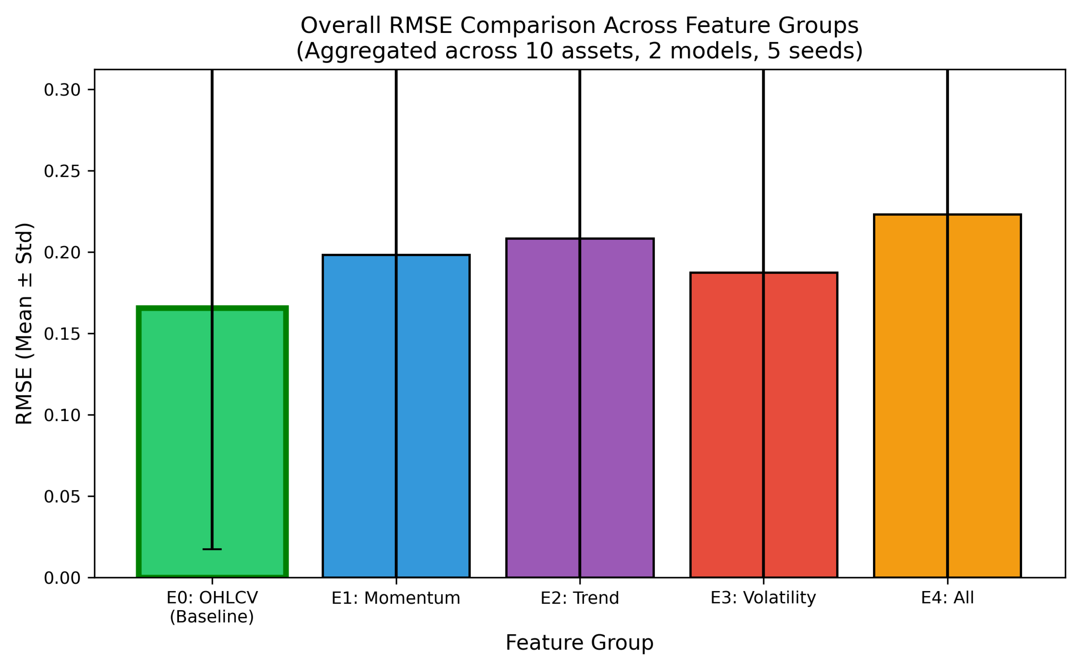
Figure 6. RMSE comparison across feature groups, showing mean performance degradation relative to the OHLCV baseline (E0). Each bar represents the average RMSE increase across all assets and architectures; error bars indicate ±1 standard deviation. The baseline achieves the lowest prediction error, while the all-indicators configuration (E4) exhibits the largest degradation. Among augmented configurations, volatility indicators (E3) show the smallest increase.

Figure 6. RMSE comparison across feature groups, showing mean performance degradation relative to the OHLCV baseline (E0). Each bar represents the average RMSE increase across all assets and architectures; error bars indicate ±1 standard deviation. The baseline achieves the lowest prediction error, while the all-indicators configuration (E4) exhibits the largest degradation. Among augmented configurations, volatility indicators (E3) show the smallest increase.

6.3. Indicator Category Ranking

Finding.

No indicator category improves upon the baseline on average; volatility indicators produce the smallest degradation.

Ranking configurations by mean RMSE degradation relative to the baseline:

1.

E3 (Volatility, 4 indicators): $+13.1\%$ degradation.

2.

E1 (Momentum, 3 indicators): $+19.7\%$ degradation.

3.

E2 (Trend, 6 indicators): $+25.8\%$ degradation.

4.

E4 (All indicators, 13 total): $+34.6\%$ degradation.

Notably, the all-indicators configuration (E4) performs worst despite having the richest feature set, suggesting that combining indicators introduces redundancy and noise rather than complementary signal.

6.4. Asset Class Analysis

Finding.

Performance varies substantially across asset classes: foreign exchange achieves the lowest absolute RMSE but near-random directional accuracy.

Table 5 presents performance aggregated by asset class over all feature configurations and architectures.

Table 5. Forecasting performance by asset class. Results are aggregated across all feature configurations and architectures (100 experiments per category: 2 assets × 5 configurations × 2 architectures × 5 random seeds). Foreign exchange achieves the lowest RMSE but near-random directional accuracy (49.8%), while cryptocurrencies exhibit the highest directional accuracy (55.7%). High-volatility asset classes (commodities, cryptocurrencies) exhibit 83% higher mean RMSE than low-volatility classes.

Asset Class	RMSE	MAE	DA (%)
Commodity	0.381 ± 0.368	0.330 ± 0.320	53.3 ± 6.8
Cryptocurrency	0.158 ± 0.106	0.147 ± 0.105	55.7 ± 4.4
Equity	0.213 ± 0.022	0.201 ± 0.021	53.3 ± 3.6
Foreign Exchange	0.049 ± 0.027	0.045 ± 0.028	49.8 ± 1.8
Market Index	0.182 ± 0.017	0.173 ± 0.017	53.8 ± 2.9
Aggregated by volatility regime:
High volatility (Commodity, Crypto)	RMSE = 0.270, DA = 54.5%
Low volatility (Equity, Forex, Index)	RMSE = 0.148, DA = 52.3%

Table 5. Forecasting performance by asset class. Results are aggregated across all feature configurations and architectures (100 experiments per category: 2 assets × 5 configurations × 2 architectures × 5 random seeds). Foreign exchange achieves the lowest RMSE but near-random directional accuracy (49.8%), while cryptocurrencies exhibit the highest directional accuracy (55.7%). High-volatility asset classes (commodities, cryptocurrencies) exhibit 83% higher mean RMSE than low-volatility classes.

Asset Class	RMSE	MAE	DA (%)
Commodity	0.381 ± 0.368	0.330 ± 0.320	53.3 ± 6.8
Cryptocurrency	0.158 ± 0.106	0.147 ± 0.105	55.7 ± 4.4
Equity	0.213 ± 0.022	0.201 ± 0.021	53.3 ± 3.6
Foreign Exchange	0.049 ± 0.027	0.045 ± 0.028	49.8 ± 1.8
Market Index	0.182 ± 0.017	0.173 ± 0.017	53.8 ± 2.9
Aggregated by volatility regime:
High volatility (Commodity, Crypto)	RMSE = 0.270, DA = 54.5%
Low volatility (Equity, Forex, Index)	RMSE = 0.148, DA = 52.3%

The main observations by asset class are as follows:

• Foreign exchange achieves the lowest mean RMSE ($0.049\pm 0.027$), most likely because of the lower volatility and narrower price ranges of currency pairs. Directional accuracy (49.8%), however, is statistically indistinguishable from random, indicating that while the models predict price levels well, they fail to capture directional movements.
• Cryptocurrencies show moderate RMSE (0.158) coupled with the highest directional accuracy (55.7%), possibly reflecting stronger momentum patterns that recurrent networks are able to exploit.
• Commodities exhibit the highest variance ($0.381\pm 0.368$), driven by the large disparity between crude oil (which shows extreme outlier behaviour) and gold.
• High-volatility assets (cryptocurrencies and commodities combined) have 83% higher mean RMSE than low-volatility assets (equities, forex, indices): 0.270 versus 0.148.

Volatility indicator impact by asset class.

Table 6 reports the effect of volatility indicators (E3) relative to the baseline (E0) for each asset class.

Table 6. Impact of volatility indicators (E3) relative to the OHLCV baseline (E0) by asset class. $\mathrm{\Delta }$RMSE is computed as percentage change; positive values indicate RMSE reduction (improvement), negative values indicate RMSE increase (degradation). Foreign exchange is the sole asset class where volatility indicators improve forecasting performance.

Asset Class	$\mathit{\Delta }$RMSE	Improvement?
Commodity	$-32.4\%$	No
Cryptocurrency	$-7.1\%$	No
Equity	$-0.3\%$	No
Foreign Exchange	$+4.2\%$	Yes
Market Index	$-4.9\%$	No

Note: Foreign exchange is the only asset class where volatility indicators improve performance.

Table 6. Impact of volatility indicators (E3) relative to the OHLCV baseline (E0) by asset class. $\mathrm{\Delta }$RMSE is computed as percentage change; positive values indicate RMSE reduction (improvement), negative values indicate RMSE increase (degradation). Foreign exchange is the sole asset class where volatility indicators improve forecasting performance.

Asset Class	$\mathit{\Delta }$RMSE	Improvement?
Commodity	$-32.4\%$	No
Cryptocurrency	$-7.1\%$	No
Equity	$-0.3\%$	No
Foreign Exchange	$+4.2\%$	Yes
Market Index	$-4.9\%$	No

Note: Foreign exchange is the only asset class where volatility indicators improve performance.

Foreign exchange is the only asset class in which volatility indicators improve performance (4.2% RMSE reduction). This may reflect the importance of explicit volatility features in currency markets, where volatility clustering and central bank policy regimes create more predictable dynamics. Counterintuitively, cryptocurrencies—despite their extreme volatility—show degradation ($-7.1\%$) with volatility indicators, suggesting that high baseline volatility alone does not translate to indicator utility.

6.5. Architecture Comparison: LSTM versus GRU

Finding.

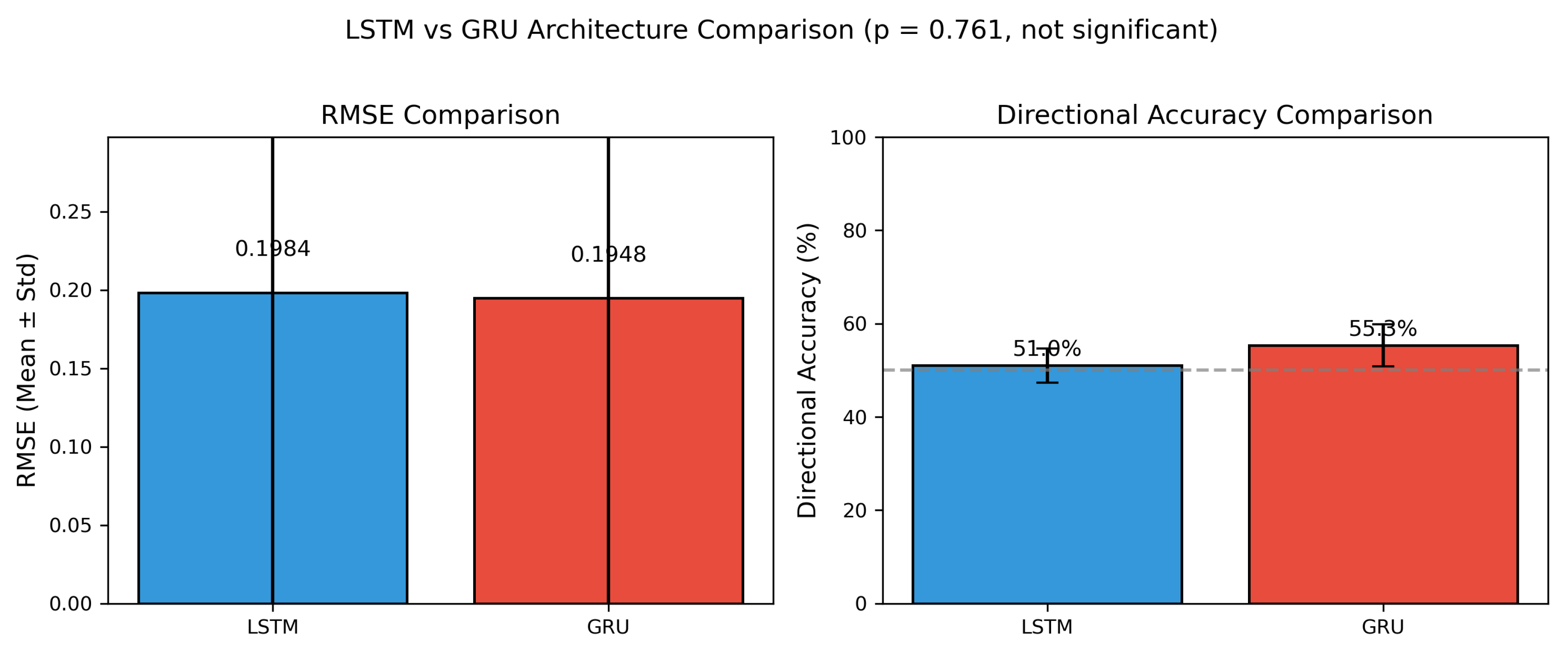
GRU marginally outperforms LSTM in directional accuracy, but the RMSE difference between the two architectures is not statistically significant.

Table 7 compares the two architectures, aggregated across all assets and feature configurations.

Table 7. Comparison of LSTM and GRU architectures. Results are aggregated across all assets and feature configurations (250 experiments per architecture: 10 assets × 5 configurations × 5 random seeds). Parameter counts are for the E0 configuration (5 input features). Despite fewer parameters, GRU achieves marginally lower RMSE and substantially higher directional accuracy, though RMSE differences do not reach statistical significance.

Architecture	RMSE	MAE	DA (%)	Parameters
LSTM	0.198 ± 0.204	0.179 ± 0.176	51.0 ± 3.7	26,817
GRU	0.195 ± 0.202	0.180 ± 0.179	55.3 ± 4.5	20,385
Statistical test (independent t-test):
$t=0.19$, $p=0.846$ (not significant), Cohen’s $d=0.017$ (negligible)

Table 7. Comparison of LSTM and GRU architectures. Results are aggregated across all assets and feature configurations (250 experiments per architecture: 10 assets × 5 configurations × 5 random seeds). Parameter counts are for the E0 configuration (5 input features). Despite fewer parameters, GRU achieves marginally lower RMSE and substantially higher directional accuracy, though RMSE differences do not reach statistical significance.

Architecture	RMSE	MAE	DA (%)	Parameters
LSTM	0.198 ± 0.204	0.179 ± 0.176	51.0 ± 3.7	26,817
GRU	0.195 ± 0.202	0.180 ± 0.179	55.3 ± 4.5	20,385
Statistical test (independent t-test):
$t=0.19$, $p=0.846$ (not significant), Cohen’s $d=0.017$ (negligible)

• GRU achieves lower mean RMSE ($0.195\pm 0.202$ versus $0.198\pm 0.204$).
• GRU achieves higher mean directional accuracy ($55.3\%\pm 4.5\%$ versus $51.0\%\pm 3.7\%$).
• Independent t-test: $t=0.19$, $p=0.846$ (not significant at $\alpha =0.05$).
• Effect size: Cohen’s $d=0.017$ (negligible).

Despite its simpler architecture (roughly 24% fewer parameters), GRU performs comparably to LSTM in terms of RMSE. The directional accuracy advantage for GRU, while sizable in magnitude, warrants further investigation to determine whether it reflects a genuine architectural advantage or is an artefact of the particular datasets studied.

6.6. Evidence of Feature Redundancy

Finding.

Combining all indicators produces the worst performance, indicating redundancy and noise accumulation rather than signal complementarity.

The progressive degradation from single-category indicators to the comprehensive combination follows a consistent pattern:

• E3 (4 volatility indicators): $+13.1\%$ RMSE degradation
• E1 (3 momentum indicators): $+19.7\%$ RMSE degradation
• E2 (6 trend indicators): $+25.8\%$ RMSE degradation
• E4 (13 total indicators): $+34.6\%$ RMSE degradation

The all-indicators configuration (E4) performs substantially worse than any single-category configuration, despite containing a superset of their features. This pattern suggests:

1.

Inter-indicator redundancy: Multiple indicators derived from similar price relationships (e.g., SMA and EMA, or RSI and Stochastic) are highly correlated, providing duplicative rather than complementary information.

2.

Noise accumulation: Each indicator introduces additional variance that compounds across the feature set without proportional signal gain.

3.

Increased model complexity: Higher-dimensional input spaces require learning more parameters, potentially increasing overfitting risk given fixed training set sizes.

6.7. Best Configurations by Asset

Table 8 identifies the optimal configuration for each asset, selected by minimum test-set RMSE.

Table 8. Optimal configuration for each asset, selected by minimum test-set RMSE across all 50 configurations per asset (5 feature groups × 2 architectures × 5 random seeds). Five assets achieve best performance with the baseline OHLCV configuration (E0), three prefer volatility indicators (E3), and two prefer all indicators (E4). GRU is selected for 6 of 10 assets. Bold RMSE indicates minimum across all assets; bold DA indicates maximum.

Category	Asset	Model	Best Config.	RMSE	DA (%)
Commodity	Crude Oil	GRU	E4: All	0.016	47.8
	Gold	LSTM	E0: OHLCV	0.453	58.2
Cryptocurrency	Bitcoin	LSTM	E0: OHLCV	0.181	54.2
	Ethereum	GRU	E3: Volatility	0.045	58.3
Equity	Apple	GRU	E0: OHLCV	0.175	61.5
	Microsoft	LSTM	E3: Volatility	0.171	50.8
Forex	EUR/USD	GRU	E4: All	0.019	49.7
	USD/JPY	LSTM	E3: Volatility	0.045	50.8
Index	NASDAQ	GRU	E0: OHLCV	0.152	57.5
	S&P 500	GRU	E0: OHLCV	0.168	58.2

Table 8. Optimal configuration for each asset, selected by minimum test-set RMSE across all 50 configurations per asset (5 feature groups × 2 architectures × 5 random seeds). Five assets achieve best performance with the baseline OHLCV configuration (E0), three prefer volatility indicators (E3), and two prefer all indicators (E4). GRU is selected for 6 of 10 assets. Bold RMSE indicates minimum across all assets; bold DA indicates maximum.

Category	Asset	Model	Best Config.	RMSE	DA (%)
Commodity	Crude Oil	GRU	E4: All	0.016	47.8
	Gold	LSTM	E0: OHLCV	0.453	58.2
Cryptocurrency	Bitcoin	LSTM	E0: OHLCV	0.181	54.2
	Ethereum	GRU	E3: Volatility	0.045	58.3
Equity	Apple	GRU	E0: OHLCV	0.175	61.5
	Microsoft	LSTM	E3: Volatility	0.171	50.8
Forex	EUR/USD	GRU	E4: All	0.019	49.7
	USD/JPY	LSTM	E3: Volatility	0.045	50.8
Index	NASDAQ	GRU	E0: OHLCV	0.152	57.5
	S&P 500	GRU	E0: OHLCV	0.168	58.2

Several patterns emerge from this analysis:

• Baseline dominance: 5 of 10 assets (Gold, Bitcoin, Apple, NASDAQ, S&P 500) perform best with the raw OHLCV baseline (E0), requiring no technical indicators at all.
• Volatility indicator utility: 3 of 10 assets (Ethereum, Microsoft, USD/JPY) achieve their best results with volatility indicators (E3).
• All-indicators configuration: 2 of 10 assets (Crude Oil, EUR/USD) favour the full indicator set (E4).
• GRU preference: 6 of 10 assets achieve their best results with GRU rather than LSTM.
• Highest directional accuracy: Apple with GRU and baseline features reaches 61.5% directional accuracy—substantially above the 50% random baseline.

6.8. Visualisation

Figure 7 illustrates RMSE across feature configurations for Bitcoin, a representative cryptocurrency asset.

Figure 7. RMSE comparison across feature configurations for Bitcoin (BTC/USD). Each bar represents the mean RMSE over five random seeds; error bars indicate ±1 standard deviation. The baseline OHLCV configuration (E0) is competitive with or superior to all indicator-augmented variants. E0: OHLCV only; E1: Momentum; E2: Trend; E3: Volatility; E4: All indicators combined.

Figure 7. RMSE comparison across feature configurations for Bitcoin (BTC/USD). Each bar represents the mean RMSE over five random seeds; error bars indicate ±1 standard deviation. The baseline OHLCV configuration (E0) is competitive with or superior to all indicator-augmented variants. E0: OHLCV only; E1: Momentum; E2: Trend; E3: Volatility; E4: All indicators combined.

Figure 8 presents the relative performance change compared to the baseline for the S&P 500, illustrating the consistent degradation pattern.

Figure 8. Percentage change in RMSE relative to the OHLCV baseline (E0) for the S&P 500 index. Positive values indicate performance degradation (higher RMSE). All four indicator-augmented configurations underperform the raw price baseline for this market index, with trend indicators (E2) showing the largest degradation.

Figure 8. Percentage change in RMSE relative to the OHLCV baseline (E0) for the S&P 500 index. Positive values indicate performance degradation (higher RMSE). All four indicator-augmented configurations underperform the raw price baseline for this market index, with trend indicators (E2) showing the largest degradation.

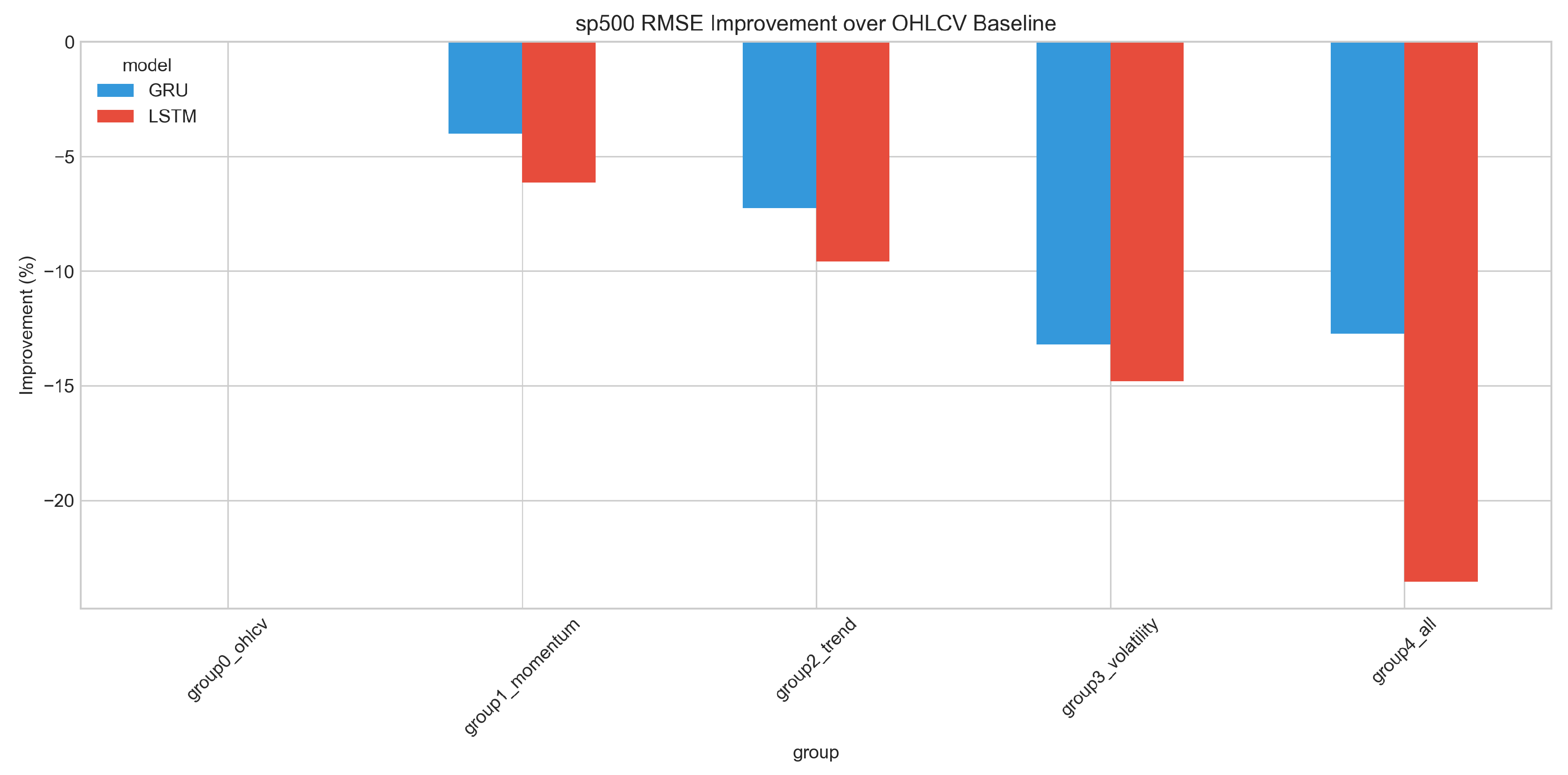
Figure 9 provides a performance heatmap for Apple, enabling visual comparison across architectures and feature configurations.

Figure 9. Performance heatmap for Apple Inc. (AAPL) showing test-set RMSE across model architectures (rows) and feature configurations (columns). Darker shading corresponds to lower RMSE (better performance). The GRU with baseline OHLCV features achieves the lowest prediction error (RMSE = 0.175) for this equity.

Figure 9. Performance heatmap for Apple Inc. (AAPL) showing test-set RMSE across model architectures (rows) and feature configurations (columns). Darker shading corresponds to lower RMSE (better performance). The GRU with baseline OHLCV features achieves the lowest prediction error (RMSE = 0.175) for this equity.

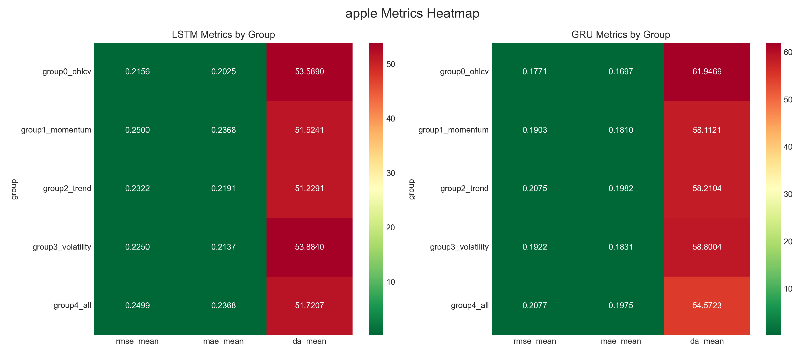
6.9. Summary of Principal Findings

The experimental results lead to the following key conclusions:

1.

Technical indicators do not improve deep learning forecasting performance on average; all four indicator categories show statistically significant degradation relative to the baseline.

2.

The comprehensive all-indicators configuration exhibits the worst performance ($+34.6\%$ RMSE increase, $p<0.001$), providing clear evidence of feature redundancy rather than complementarity.

3.

Among augmented configurations, volatility indicators show the smallest degradation overall and are the only indicators that improve performance for a specific asset class—foreign exchange (4.2% RMSE reduction).

4.

LSTM and GRU perform comparably, with no statistically significant RMSE difference ($p=0.846$), although GRU achieves higher directional accuracy.

5.

Performance differs markedly by asset class: high-volatility assets exhibit 83% higher prediction error than low-volatility assets.

6.

The baseline OHLCV configuration achieves optimal or near-optimal performance for the majority of assets tested.

7. Discussion

This section interprets the experimental findings, examines possible explanatory mechanisms, discusses implications for both research and practice, acknowledges limitations, and identifies directions for future work.

7.1. Interpretation of Results

7.1.1. Why Do Technical Indicators Degrade Performance?

The finding that technical indicators degrade deep learning forecasting performance may seem counterintuitive, given how widely these features are used in quantitative finance. Several mechanisms can account for this result.

Information redundancy.

Technical indicators are deterministic transformations of the underlying OHLCV data. LSTM and GRU networks have sufficient representational capacity to learn nonlinear functions of their inputs; if the patterns captured by indicators are already learnable from raw data, the explicit indicator features carry no additional information. Worse, the network may instead model indicator-induced correlations that do not generalise to unseen data (see Figure 4).

Noise introduction.

Each indicator involves hyperparameters—lookback periods, smoothing constants—that are set by historical convention rather than optimised for the specific prediction task at hand. These fixed parameters can introduce artefacts that interfere with learning. Indicators computed during unusual market conditions (e.g., low liquidity or price gaps) may also produce outlier values that increase training variance.

Curse of dimensionality.

Increasing the feature count from 5 (OHLCV) to 18 (all indicators) substantially expands the input space. With training set sizes held fixed, higher-dimensional representations lead to sparser sampling of the feature space, which can hurt generalisation.

Implicit feature learning.

One of the principal advantages of deep learning is its capacity for automatic feature extraction from raw data. When handcrafted indicators are provided, the model may overweight these explicit features at the expense of patterns it would otherwise discover on its own. If the handcrafted features are suboptimal for the prediction task, this inductive bias harms performance.

Temporal smoothing.

Many indicators (moving averages, ADX, RSI) involve temporal smoothing that attenuates high-frequency variation. While smoothing is useful for visual analysis and rule-based trading, it may also remove information relevant to next-day prediction.

7.1.2. Why Does the All-Indicators Configuration Perform Worst?

The E4 configuration, which combines all 13 indicators, exhibits the largest performance degradation (34.6% RMSE increase; see Figure 6). This outcome is consistent with several interacting effects:

• Accumulated redundancy: indicators within the same family (e.g., SMA and EMA; RSI and Stochastic) are highly correlated, contributing duplicative information that inflates parameter counts without proportional signal.
• Noise compounding: measurement noise and indicator-specific artefacts from each feature accumulate rather than cancel, raising the overall variance of the input representation.
• Capacity dilution: with more input dimensions, the model must spread its representational capacity across a larger feature set, potentially diluting attention to the most informative signals.
• Conflicting signals: different indicator categories may suggest contradictory market states—momentum indicators might signal mean-reversion while trend indicators signal continuation—creating confusion during learning.

7.1.3. Why Does Foreign Exchange Benefit from Volatility Indicators?

Foreign exchange is the only asset class where volatility indicators improve performance (4.2% RMSE reduction). Several features of currency markets may explain this result:

• Volatility clustering: currency pairs exhibit pronounced volatility persistence (GARCH effects), making explicit volatility measures informative about near-term price dynamics.
• Policy-driven regimes: central bank interventions and monetary policy announcements create distinct volatility regimes that explicit indicators may capture more effectively than raw prices alone.
• Lower baseline volatility: with lower absolute volatility than cryptocurrencies or commodities, the signal-to-noise ratio of volatility indicators is higher in forex markets.
• Mean-reverting dynamics: major currency pairs often exhibit mean-reverting behaviour within trading ranges, and Bollinger Band position indicators (%B) may capture these dynamics effectively.

The counterintuitive finding that high-volatility assets (cryptocurrencies, commodities) do not benefit from volatility indicators deserves further scrutiny. One plausible explanation is that extreme volatility regimes are inherently unpredictable, limiting the usefulness of any backward-looking volatility measure.

7.1.4. LSTM versus GRU: Why No Significant Difference?

The comparable performance of LSTM and GRU ($p=0.846$) is consistent with prior comparative studies (see fig:lstmgrucomparison):

• Both architectures address the vanishing gradient problem through gating mechanisms.
• The LSTM’s separate cell state provides additional memory capacity that may be unnecessary for the moderate sequence lengths (60 days) and temporal dependencies typical of daily financial data.
• At daily sampling frequency, extreme long-range dependencies spanning months or years are less critical than in domains such as natural language processing.

GRU’s marginally higher directional accuracy (55.3% versus 51.0%) with fewer parameters suggests potential efficiency advantages, though this difference needs to be replicated before firm conclusions can be drawn.

7.2. Assessment of Prior Expectations

The experimental results can be evaluated against several hypotheses that would be reasonable to formulate on the basis of prior literature and practitioner experience.

Hypothesis 1: Technical indicators enhance model performance.

Traditional technical analysis holds that indicators extract predictive signal from price history. Our results reject this hypothesis in the present context: the baseline configuration outperforms every indicator-augmented variant on average, and all four indicator categories exhibit statistically significant degradation. This suggests that the representational capacity of recurrent neural networks effectively subsumes the information content of standard technical indicators.

Hypothesis 2: Different asset classes benefit from different indicator types.

The data provide partial support for this hypothesis. Optimal configurations do vary across asset classes—foreign exchange benefits from volatility indicators, while equities and indices favour the baseline. Nevertheless, no asset class shows consistent improvement from any indicator category across all metrics and configurations, suggesting that the relationship between asset characteristics and indicator utility is weaker than intuition might suggest.

Hypothesis 3: Volatility indicators benefit high-volatility assets.

Contrary to this seemingly natural expectation, the most volatile assets (cryptocurrencies) show degradation with volatility indicators ($-7.1\%$), while foreign exchange—with comparatively lower volatility—is the sole beneficiary ($+4.2\%$). This inversion implies that indicator utility depends more on market microstructure than on raw volatility levels.

Hypothesis 4: Comprehensive indicator combinations achieve superior performance.

This hypothesis is strongly rejected. The all-indicators configuration (E4) exhibits the worst performance ($+34.6\%$ degradation, $p<0.001$, $d=-0.29$). Rather than providing complementary information, comprehensive indicator sets appear to introduce cumulative noise and redundancy.

Hypothesis 5: LSTM outperforms GRU due to its additional memory capacity.

We find no evidence of LSTM superiority; the RMSE difference is not statistically significant ($p=0.846$, Cohen’s $d=0.017$). For daily financial forecasting with 60-day lookback windows, GRU’s simpler architecture achieves equivalent prediction accuracy with fewer parameters and faster training.

7.3. Relation to Prior Literature

The present findings can be situated within the broader literature on feature engineering for financial deep learning, where they reinforce certain prior observations while contradicting others.

Bao et al. (2017).

These authors reported improvements using wavelet transforms, stacked autoencoders, and LSTM with indicator features [8]. The key architectural differences—wavelet preprocessing for denoising and autoencoder-based feature learning—may enable more effective utilisation of indicator information than standard recurrent networks. Our results suggest that those preprocessing stages, rather than the indicators themselves, may be the primary driver of the reported improvements.

Nelson et al. (2017).

Nelson and colleagues reported 55.9% directional accuracy using 180 technical indicator features with LSTM on Brazilian equities [9]. Crucially, their study did not include a raw-price baseline, leaving open whether indicators contributed predictive value beyond what an LSTM could extract from price data alone. Our controlled ablation directly addresses this gap.

Selvin et al. (2017).

Selvin and colleagues observed benefits with CNN, RNN, and LSTM using shorter sliding windows and indicator features on Indian stocks [10]. Shorter lookback periods and different preprocessing choices may alter the relative utility of indicators. Notably, they too observed non-uniform performance across stocks, consistent with the asset-specific heterogeneity we document more extensively.

Chong et al. (2017).

Chong, Han, and Park found comparable performance between raw returns and indicator-augmented inputs for deep feedforward networks on Korean equities [11], providing the closest precedent for our finding that deep networks render indicators redundant. Our study extends this observation to recurrent architectures across five asset classes, demonstrating that redundancy is a cross-market phenomenon rather than a single-market artefact.

Patel et al. (2015).

Patel and colleagues showed that trend-deterministic indicator representations outperformed raw indicator values for classical ML classifiers [30]. Their finding—that input encoding matters more than indicator selection—is consistent with our observation that how features are presented to the model, rather than the sheer volume of features, determines predictive utility.

Methodological positioning.

Following the large-scale evaluation approach advocated by Gu, Kelly, and Xiu [25], the present study offers several methodological advantages over the works cited above: (1) multi-asset, multi-class coverage enabling assessment of generalisability; (2) a controlled ablation design with a consistent OHLCV baseline; (3) statistical rigour through multiple random seeds, paired significance testing, and effect size quantification [33,34]; and (4) systematic indicator categorisation that distinguishes momentum, trend, and volatility effects.

7.4. Practical Implications

7.4.1. For Trading System Developers

1.

Establish baselines first. Raw OHLCV data should serve as the default starting point. Technical indicators should only be added when rigorous validation on held-out data demonstrates consistent improvement.

2.

Evaluate on an asset-specific basis. Indicator utility varies by asset class. Volatility indicators may benefit foreign exchange models while offering no advantage for equities or cryptocurrencies.

3.

Resist feature proliferation. Adding more indicators generally degrades performance. When using indicators, a small set of uncorrelated features is preferable to a comprehensive indicator suite.

4.

Consider GRU for efficiency. With prediction accuracy comparable to LSTM and fewer parameters, GRU offers faster training and may be preferable for deployment.

5.

Validate rigorously. Indicator benefits should not be assumed on the basis of prior literature or intuition. Each proposed feature should be tested explicitly against an OHLCV baseline using proper train/validation/test splits and multiple random seeds.

7.4.2. For Researchers

1.

Report baseline comparisons. Studies proposing new feature engineering approaches should benchmark against OHLCV baselines, not only against alternative indicator configurations.

2.

Use statistical testing. Results should be reported across multiple random seeds, accompanied by significance tests and effect sizes, rather than relying on single-run comparisons.

3.

Evaluate across assets. Findings from a single asset may not generalise. Multi-asset studies provide stronger foundations for robust conclusions.

4.

Publish null and negative results. Evidence that indicators do not improve performance is scientifically valuable and helps counteract publication bias in the literature.

7.5. Theoretical Implications

The results have broader implications for understanding the role of feature engineering in deep learning.

Deep learning as feature learner.

Our findings support the view that deep recurrent networks are effective automatic feature extractors, consistent with evidence from Sirignano and Cont [27] that deep models can discover universal price formation features directly from raw market data. When models possess sufficient capacity and training data, handcrafted features derived from the same underlying signals may constrain rather than enhance learning.

Domain knowledge integration.

If explicit indicator features do not improve performance, it is worth asking how domain knowledge can be incorporated more effectively. Architectural choices (attention mechanisms, hierarchical structures), task-specific loss function design (directional penalties, regime-aware objectives), and domain-informed regularisation schemes may prove more fruitful than input feature engineering [28].

Market efficiency considerations.

The results are broadly consistent with the weak form of the Efficient Market Hypothesis [15] and with Lo’s Adaptive Markets framework [20]: standard technical indicators, which are widely known and computationally trivial, may be substantially “priced in” by modern markets, leaving little exploitable edge for prediction models. The fact that foreign exchange—where central bank policy creates distinct volatility regimes—is the sole beneficiary of volatility indicators aligns with the AMH prediction that exploitable patterns persist mainly in markets with pronounced structural features.

7.6. Limitations

Several limitations scope the conclusions of this study:

1.

Temporal resolution. We analyse daily data exclusively. Intraday markets may exhibit different indicator dynamics, particularly for momentum and volatility measures.

2.

Prediction horizon. The study is restricted to one-day-ahead prediction. Longer horizons (weekly, monthly) or multi-step forecasting may favour different feature configurations.

3.

Indicator coverage. Although our set covers the major categories, it is not exhaustive. Adaptive indicators, alternative oscillators, or market-specific measures may behave differently.

4.

Market regime coverage. The study period (2010–2025) encompasses diverse market conditions but may not include every regime type. Indicator utility may be state-dependent in ways not captured by aggregate analysis.

5.

Architecture scope. We evaluate standard LSTM and GRU configurations. Attention-based models (Transformers, Temporal Fusion Transformers) may interact with indicator features differently.

6.

Hyperparameter sensitivity. Indicator parameters (lookback periods) are fixed at conventional values. Jointly optimising indicator and model hyperparameters could alter the conclusions.

7.

Alternative targets. We predict raw closing prices. Indicators may prove more useful for alternative targets such as volatility forecasting, regime classification, or return prediction.

7.7. Future Research Directions

Building on these findings and their limitations, we identify several promising avenues for further investigation:

1.

Learnable indicators. Develop indicators whose parameters are optimised jointly with model weights during training, enabling end-to-end learning of feature transformations tailored to the prediction task.

2.

Regime-conditional features. Investigate whether indicators provide benefits in specific market regimes (trending versus ranging, high versus low volatility) through conditional or regime-switching models.

3.

Attention-based architectures. Evaluate whether Transformer and Temporal Fusion architectures [28] can more effectively leverage indicator features through attention mechanisms that weight feature importance dynamically.

4.

Higher-frequency analysis. Extend the methodology to intraday data, where indicator calculation windows, market microstructure, and prediction horizons differ substantially from the daily setting.

5.

Multi-task learning. Explore whether indicators benefit auxiliary prediction tasks (volatility forecasting, regime classification) even when they do not improve price prediction.

6.

Interpretability analysis. Apply feature attribution methods (SHAP, integrated gradients, attention visualisation) to understand how deep learning models utilise raw versus derived features.

8. Conclusion

This paper has presented a controlled empirical investigation into the impact of technical indicators on deep learning-based financial time series forecasting. Through 500 experiments spanning 10 assets across five asset classes, five feature configurations, two recurrent architectures, and five random seeds, we provide statistically rigorous evidence addressing a fundamental question in quantitative finance and applied machine learning.

8.1. Principal Findings

The experimental results support seven principal conclusions:

1.

Technical indicators degrade forecasting performance. Contrary to conventional practice, indicator-augmented feature sets increase prediction error relative to raw OHLCV data. The baseline configuration achieves the lowest mean RMSE ($0.166\pm 0.148$) and the highest mean directional accuracy ($55.7\%\pm 5.5\%$).

2.

All four indicator categories produce statistically significant degradation. Momentum ($p<0.001$), trend ($p<0.001$), volatility ($p=0.005$), and the combined configuration ($p<0.001$) all exhibit significantly higher RMSE than the baseline.

3.

Combining indicators yields the worst performance. The comprehensive E4 configuration, comprising 13 indicators, incurs a 34.6% RMSE increase, indicating that feature combination introduces redundancy and noise rather than complementary signal.

4.

Volatility indicators provide an asset-class-specific benefit. Foreign exchange is the sole asset class where volatility indicators improve performance (4.2% RMSE reduction), plausibly reflecting the importance of volatility regimes in currency markets.

5.

High-volatility assets are harder to predict. Cryptocurrencies and commodities show 83% higher mean RMSE than equities, forex, and indices, consistent with the greater difficulty of forecasting volatile price series.

6.

LSTM and GRU perform comparably. No statistically significant RMSE difference exists between architectures ($p=0.846$, Cohen’s $d=0.017$), though GRU achieves modestly higher directional accuracy with fewer parameters.

7.

Simple configurations often dominate. Five of ten assets achieve optimal performance with the OHLCV baseline alone, requiring no technical indicators.

8.2. Contributions

This work offers contributions along four dimensions:

Empirical contribution.

We provide a large-scale ablation study of technical indicator impact across diverse asset classes, addressing a gap in prior literature that has focused predominantly on single assets or markets.

Methodological contribution.

The experimental design—employing multiple random seeds, paired statistical tests, and effect size quantification—offers a replicable template for rigorous comparative studies in financial machine learning.

Practical contribution.

The findings yield actionable guidance for practitioners: establish OHLCV baselines, validate indicator benefits rigorously, resist feature proliferation, and consider GRU for computational efficiency.

Theoretical contribution.

The results support the view that deep recurrent networks function as effective automatic feature extractors, potentially rendering handcrafted technical indicators redundant for next-day price prediction.

8.3. Recommendations

For trading system developers.

• Begin with OHLCV baseline features; add indicators only when validation evidence demonstrates improvement.
• Evaluate volatility indicators specifically for foreign exchange applications.
• Limit indicator count to minimise noise accumulation.
• Consider GRU architecture for comparable accuracy at reduced computational cost.

For researchers.

• Benchmark proposed methods against OHLCV baselines, not only against other indicator configurations.
• Report results from multiple random seeds with statistical significance testing.
• Evaluate across multiple asset classes to assess generalisability.
• Publish null and negative findings to help counteract publication bias.

8.4. Scope and Limitations

These conclusions are scoped to the experimental conditions studied: daily OHLCV data, one-day-ahead price prediction, standard LSTM and GRU architectures, and conventional indicator parameters. Extensions to intraday data, longer prediction horizons, attention-based architectures, or jointly optimised indicator parameters may reveal different patterns, and these constitute important directions for future work.

8.5. Concluding Remarks

These findings challenge a foundational assumption in quantitative finance: that technical indicators derived from historical prices provide valuable predictive signal. While this may hold for traditional statistical models with limited feature-learning capacity, modern deep recurrent networks appear capable of extracting equivalent or superior representations directly from raw price data.

This does not imply that technical analysis lacks merit for human interpretation, discretionary trading, or risk management. For practitioners developing automated forecasting systems with deep neural networks, however, the evidence suggests that simplicity may be preferable to feature engineering complexity. The burden of proof should rest with those proposing to add handcrafted features, not with those employing parsimonious input representations.

We hope this study provides a rigorous empirical foundation for feature engineering decisions in deep learning-based financial forecasting and contributes to more evidence-driven practices in applied quantitative finance.

References

- Cont, R. Empirical properties of asset returns: Stylized facts and statistical issues. Quantitative Finance 2001, 1, 223–236. [Google Scholar] [CrossRef]
- Sezer, O.B.; Gudelek, M.U.; Ozbayoglu, A.M. Financial time series forecasting with deep learning: A systematic literature review: 2005–2019. Applied Soft Computing 2020, 90, 106181. [Google Scholar] [CrossRef]
- Hochreiter, S.; Schmidhuber, J. Long short-term memory. Neural Computation 1997, 9, 1735–1780. [Google Scholar] [CrossRef]
- Cho, K.; Van Merriënboer, B.; Gulcehre, C.; Bahdanau, D.; Bougares, F.; Schwenk, H.; Bengio, Y. Learning phrase representations using RNN encoder-decoder for statistical machine translation. In Proceedings of the Proceedings of the 2014 Conference on Empirical Methods in Natural Language Processing (EMNLP), 2014; pp. 1724–1734. [Google Scholar]
- Fischer, T.; Krauss, C. Deep learning with long short-term memory networks for financial market predictions. European Journal of Operational Research 2018, 270, 654–669. [Google Scholar] [CrossRef]
- Murphy, J.J. Technical Analysis of the Financial Markets: A Comprehensive Guide to Trading Methods and Applications; New York Institute of Finance, 1999. [Google Scholar]
- Achelis, S.B. Technical Analysis from A to Z; McGraw-Hill, 2001. [Google Scholar]
- Bao, W.; Yue, J.; Rao, Y. A deep learning framework for financial time series using stacked autoencoders and long-short term memory. PLoS ONE 2017, 12, e0180944. [Google Scholar] [CrossRef]
- Nelson, D.M.Q.; Pereira, A.C.M.; de Oliveira, R.A. Stock market’s price movement prediction with LSTM neural networks. In Proceedings of the 2017 International Joint Conference on Neural Networks (IJCNN), 2017; IEEE; pp. 1419–1426. [Google Scholar]
- Selvin, S.; Vinayakumar, R.; Gopalakrishnan, E.; Menon, V.K.; Soman, K. Stock price prediction using LSTM, RNN and CNN-sliding window model. In Proceedings of the 2017 International Conference on Advances in Computing, Communications and Informatics (ICACCI), 2017; IEEE; pp. 1643–1647. [Google Scholar]
- Chong, E.; Han, C.; Park, F.C. Deep learning networks for stock market analysis and prediction: Methodology, data representations, and case studies. Expert Systems with Applications 2017, 83, 187–205. [Google Scholar] [CrossRef]
- Cao, J.; Li, Z.; Li, J. Financial time series forecasting model based on CEEMDAN and LSTM. Physica A: Statistical Mechanics and its Applications 2019, 519, 127–139. [Google Scholar] [CrossRef]
- Zhang, L.; Aggarwal, C.; Kong, X.; Philip, S.Y. Stock price prediction via discovering multi-frequency trading patterns. In Proceedings of the 23rd ACM SIGKDD International Conference on Knowledge Discovery and Data Mining, 2017; pp. 2141–2149. [Google Scholar]
- Nti, I.K.; Adekoya, A.F.; Weyori, B.A. A systematic review of fundamental and technical analysis of stock market predictions. Artificial Intelligence Review 2020, 53, 3007–3057. [Google Scholar] [CrossRef]
- Fama, E.F. Efficient capital markets: A review of theory and empirical work. The Journal of Finance 1970, 25, 383–417. [Google Scholar] [CrossRef]
- Fama, E.F.; Blume, M.E. Filter rules and stock-market trading. The Journal of Business 1966, 39, 226–241. [Google Scholar] [CrossRef]
- Lo, A.W.; Mamaysky, H.; Wang, J. Foundations of technical analysis: Computational algorithms, statistical inference, and empirical implementation. The Journal of Finance 2000, 55, 1705–1765. [Google Scholar] [CrossRef]
- Brock, W.; Lakonishok, J.; LeBaron, B. Simple technical trading rules and the stochastic properties of stock returns. The Journal of Finance 1992, 47, 1731–1764. [Google Scholar] [CrossRef]
- Neely, C.; Weller, P.; Dittmar, R. Is technical analysis in the foreign exchange market profitable? A genetic programming approach. Journal of Financial and Quantitative Analysis 1997, 32, 405–426. [Google Scholar] [CrossRef]
- Lo, A.W. The adaptive markets hypothesis. The Journal of Portfolio Management 2004, 30, 15–29. [Google Scholar] [CrossRef]
- Tsay, R.S. Analysis of Financial Time Series, 3rd ed.; John Wiley & Sons, 2010. [Google Scholar]
- LeCun, Y.; Bengio, Y.; Hinton, G. Deep learning. Nature 2015, 521, 436–444. [Google Scholar] [CrossRef]
- Chung, J.; Gulcehre, C.; Cho, K.; Bengio, Y. Empirical evaluation of gated recurrent neural networks on sequence modeling. In Proceedings of the NIPS 2014 Workshop on Deep Learning, 2014. [Google Scholar]
- Greff, K.; Srivastava, R.K.; Koutník, J.; Steunebrink, B.R.; Schmidhuber, J. LSTM: A search space odyssey. IEEE Transactions on Neural Networks and Learning Systems 2017, 28, 2222–2232. [Google Scholar] [CrossRef]
- Gu, S.; Kelly, B.; Xiu, D. Empirical asset pricing via machine learning. The Review of Financial Studies 2020, 33, 2223–2273. [Google Scholar] [CrossRef]
- Krauss, C.; Do, X.A.; Huck, N. Deep neural networks, gradient-boosted trees, random forests: Statistical arbitrage on the S&P 500. European Journal of Operational Research 2017, 259, 689–702. [Google Scholar]
- Sirignano, J.; Cont, R. Universal features of price formation in financial markets: Perspectives from deep learning. Quantitative Finance 2019, 19, 1449–1459. [Google Scholar] [CrossRef]
- Lim, B.; Zohren, S. Time-series forecasting with deep learning: A survey. Philosophical Transactions of the Royal Society A 2021, 379, 20200209. [Google Scholar] [CrossRef]
- Kara, Y.; Boyacioglu, M.A.; Baykan, Ö.K. Predicting direction of stock price index movement using artificial neural networks and support vector machines: The sample of the Istanbul Stock Exchange. Expert Systems with Applications 2011, 38, 5311–5319. [Google Scholar] [CrossRef]
- Patel, J.; Shah, S.; Thakkar, P.; Kotecha, K. Predicting stock and stock price index movement using trend deterministic data preparation and machine learning techniques. Expert Systems with Applications 2015, 42, 259–268. [Google Scholar] [CrossRef]
- Zhong, X.; Enke, D. Forecasting daily stock market return using dimensionality reduction. Expert Systems with Applications 2019, 126, 256–268. [Google Scholar] [CrossRef]
- Hoseinzade, E.; Haratizadeh, S. CNNpred: CNN-based stock market prediction using a diverse set of variables. Expert Systems with Applications 2019, 129, 273–285. [Google Scholar] [CrossRef]
- Dietterich, T.G. Approximate statistical tests for comparing supervised classification learning algorithms. Neural Computation 1998, 10, 1895–1923. [Google Scholar] [CrossRef]
- Henderson, P.; Islam, R.; Bachman, P.; Pineau, J.; Precup, D.; Meger, D. Deep reinforcement learning that matters. In Proceedings of the Proceedings of the AAAI Conference on Artificial Intelligence, 2018; Vol. 32. [Google Scholar]
- Makridakis, S.; Spiliotis, E.; Assimakopoulos, V. Statistical and machine learning forecasting methods: Concerns and ways forward. PLoS ONE 2018, 13, e0194889. [Google Scholar] [CrossRef] [PubMed]
- Tsai, C.F.; Hsiao, Y.C. Combining multiple feature selection methods for stock prediction: Union, intersection, and multi-intersection approaches. Decision Support Systems 2010, 50, 258–269. [Google Scholar] [CrossRef]
- Kim, T.; Kim, H.K. Forecasting stock prices with a feature fusion LSTM-CNN model using different representations of the same data. PLoS ONE 2019, 14, e0212320. [Google Scholar] [CrossRef]
- Kingma, D.P.; Ba, J. Adam: A method for stochastic optimization. arXiv 2014, arXiv:1412.6980. [Google Scholar]
- Glorot, X.; Bengio, Y. Understanding the difficulty of training deep feedforward neural networks. In Proceedings of the Proceedings of the Thirteenth International Conference on Artificial Intelligence and Statistics. JMLR Workshop and Conference Proceedings, 2010; pp. 249–256. [Google Scholar]
- Cohen, J. Statistical Power Analysis for the Behavioral Sciences, 2nd ed.; Lawrence Erlbaum Associates, 1988. [Google Scholar]
Disclaimer/Publisher’s Note: The statements, opinions and data contained in all publications are solely those of the individual author(s) and contributor(s) and not of MDPI and/or the editor(s). MDPI and/or the editor(s) disclaim responsibility for any injury to people or property resulting from any ideas, methods, instructions or products referred to in the content. |
© 2026 by the authors. Licensee MDPI, Basel, Switzerland. This article is an open access article distributed under the terms and conditions of the Creative Commons Attribution (CC BY) license (http://creativecommons.org/licenses/by/4.0/).
Copyright: This open access article is published under a Creative Commons CC BY 4.0 license, which permit the free download, distribution, and reuse, provided that the author and preprint are cited in any reuse.