Submitted:
09 February 2026
Posted:
09 February 2026
Read the latest preprint version here
Abstract
Let $A\in\C^{d\times d}$ and let $W(A)$ denote its numerical range. For a bounded convex domain $\Omega\subset\C$ with $C^1$ boundary containing $\spec(A)$, consider the operator-valued boundary kernel \[ P_\Omega(\sigma,A)\;:=\;\Real\!\Bigl(n_\Omega(\sigma)\,(\sigma\Id-A)^{-1}\Bigr), \qquad \sigma\in\partial\Omega, \] where $n_\Omega(\sigma)$ is the outward unit normal at $\sigma$. For convex $\Omega$ with $W(A)\subset\Omega$, this kernel is positive definite on $\partial\Omega$ and underlies boundary-integral functional calculi and spectral-set bounds in the sense of Delyon--Delyon and Crouzeix.We analyze the opposite limiting regime $\Omega\downarrow W(A)$. Along any $C^1$ convex exhaustion $\Omega_\varepsilon\downarrow W(A)$, if $\sigma_\varepsilon\in\partial\Omega_\varepsilon$ approaches a non-spectral boundary point $\sigma_0\in\partial W(A)\setminus\spec(A)$ with convergent outward normals $n_{\Omega_\varepsilon}(\sigma_\varepsilon)\to n$, then $\lambda_{\min}(P_{\Omega_\varepsilon}(\sigma_\varepsilon,A))\to 0$ and the associated min-eigenvector directions converge (up to subsequences and phases) to the canonical subspace $(\sigma_0\Id-A)\mathcal M(n)$ determined by the maximal eigenspace of $H(n)=\Real(\overline{n}A)$.Quantitatively, we obtain two-sided bounds in terms of the support-gap scalar $\delta(\sigma,n)=\Real(\overline{n}\,\sigma)-\lambda_{\max}(H(n))$, yielding a linear degeneracy rate under bounded-resolvent hypotheses and an explicit rate for outer offsets $W(A)+\varepsilon\mathbb{D}$. Under a spectral-isolation hypothesis for $\lambda_{\max}(H(n))$, we characterize the entire collapsing eigenvalue cluster under non-tangential offsets: exactly $m=\dim\mathcal M(n)$ eigenvalues decay as $O(\varepsilon)$ with a computable slope spectrum given by the eigenvalues of an explicit Gram matrix $G(n,\sigma_0)^{-1}$, while the remaining eigenvalues stay uniformly bounded away from $0$. This yields a rigorous face detector based on counting small eigenvalues, and the rescaled cluster is intrinsic under arbitrary $C^1$ convex exhaustions after normalization by $\delta$.At spectral support points $\sigma_0\in\spec(A)\cap\partial W(A)$ we obtain a three-scale picture for nonnormal matrices: an exact $1/\varepsilon$ blow-up on $\Ker(\sigma_0\Id-A)$, an $O(\varepsilon)$ collapsing cluster on $\mathcal M(n)\ominus\Ker(\sigma_0\Id-A)$ with an explicit slope spectrum, and an $O(1)$ bulk separated from $0$. For normal matrices we compute the spectrum of $P_\Omega(\sigma,A)$ explicitly, recovering a simple dichotomy at spectral support points in terms of whether the supporting face contains multiple eigenvalues. Finally, we include reproducible numerical experiments (Python) validating the predicted slopes and splittings.
Keywords:
numerical range
; operator-valued Poisson kernel
; convex domains
; functional calculus
; boundary integral methods
1. Introduction
Let and define its numerical range by
The Toeplitz–Hausdorff theorem asserts that is a compact convex subset of (see, e.g., [1,2]). Crouzeix conjectured that is a 2-spectral set for A, i.e.,
See [3,4] for the formulation and [5] for the best known universal constant .
- Background and relation to the convex-domain functional calculus. Up to normalization conventions, a central tool in the convex-domain approach of Delyon–Delyon and Crouzeix is the operator-valued boundary kerneldefined for a bounded convex domain with boundary and . Here denotes the outward unit normal at . This kernel appears in double-layer potential representations and boundary integral operators used to obtain functional calculus bounds on convex domains [4,5,6,7,8]. For convex with , positivity/coercivity of on encodes strict separation of supporting half-planes and serves as a key structural input in such estimates [7,8,9].
- Motivation: loss of coercivity near . In applications and numerical implementations of boundary-integral calculi, one often approximates by convex supersets . It is therefore natural to ask whether coercivity of the pointwise kernel can remain uniform as . The results below show that this is impossible in general: even when the resolvent stays bounded (i.e. at non-spectral boundary points ), the smallest eigenvalue of must collapse to 0 at boundary points approaching in a fixed supporting direction.
- What is new in this paper. The existing convex-domain literature primarily exploits positivity of (1.2) for fixed domains [4,7,8,9]. Here we analyze the complementary limiting regime in which shrinks to , and we make explicit the resulting loss of coercivity of the pointwise kernel. The analysis is driven by a congruence identity and by a scalar support gap , which admits a support-function interpretation in standard convex-geometry terminology.
- We prove a qualitative degeneracy theorem (Theorem 1): along any convex exhaustion , if approaches a non-spectral boundary point with convergent outward normals , then and the limiting min-eigenvector directions lie in , where is the maximal eigenspace of .
- We establish two-sided bounds for in terms of the support gap , yielding a linear degeneracy rate under bounded-resolvent hypotheses (Lemma 3 and Corollary 3), and compute explicitly for standard outer offsets (Proposition 2).
- Under a spectral-isolation hypothesis for , we quantify the entire collapsing eigenvalue cluster: exactly eigenvalues collapse linearly with an explicit slope spectrum given by the eigenvalues of a computable Gram matrix (Proposition 7), while the remaining eigenvalues stay uniformly bounded away from 0 (Proposition 8). This yields a rigorous “face detector” based on counting eigenvalues below a threshold proportional to (Corollary 5). The same slope spectrum is shown to be intrinsic under arbitrary convex exhaustions after normalization by the support gap (Proposition 9).
- We analyze the contrasting spectral-support regime . For general matrices we obtain a three-scale splitting under non-tangential offsets: an exact blow-up on , an collapsing cluster on with an explicit slope spectrum, and an bulk separated from 0 (Proposition 12). For normal matrices we recover a simple degeneracy dichotomy at spectral support points in terms of whether the supporting face contains multiple eigenvalues (Proposition 11 and Corollary 7).
- We include reproducible numerical experiments (Python) validating the predicted slopes, splittings, and direction-dependent sensitivity profiles (Section 4.9).
- Organization.Section 2 fixes notation and recalls support-function identities. Section 3 introduces , proves the key congruence identity, and establishes quantitative support-gap bounds together with a geometric interpretation of . Section 4 contains the degeneracy theorem, quantitative corollaries, slope spectra and two-/three-scale spectral splittings (including the spectral-support regime), subspace convergence, explicit examples, and reproducible numerical tests. It concludes with a brief discussion of remaining open questions.
2. Preliminaries
We use the standard notation for disks:
Throughout, is fixed. For vectors we use . For matrices we use the induced operator norm . We write for the conjugate transpose and .
For a Hermitian matrix B, we write its eigenvalues in nondecreasing order as
and in nonincreasing order as . In particular, and .
Remark 1
(Spectrum is contained in the numerical range). One has . Indeed, if with , then . Consequently, implies for any open set .
2.1. Support Functions and the Hermitian Pencil
For unimodular (i.e. ), define the Hermitian matrix
We will later write (with ) for outward unit normals on ; in the support-function identities below and throughout, such an n simply plays the role of the unimodular direction .
Let denote its largest eigenvalue and let
denote the corresponding maximal eigenspace.
Lemma 1
(Support function of the numerical range). For every unimodular ,
Moreover, if is a unit eigenvector of associated with , then and
Proof.
For ,
Taking the maximum over yields (2.2) by Rayleigh–Ritz (see, e.g., [10]). If x is a maximizing unit vector, then attains the support functional in direction , hence lies on and satisfies the stated identity. □
2.2. Convex Domains with Boundary and Normals
We identify with in the usual way. Let be a bounded open convex set with boundary. Then for each there is a unique outward unit normal vector. This assumption is used only to guarantee that the outward unit normal exists and is unique at every boundary point, ensuring that is well-defined; no higher regularity (e.g. curvature bounds) is used. We represent the normal as a unimodular complex number with so that the supporting half-plane at is
Equivalently, by convexity one has and . Under the identification , the functional is the Euclidean inner product with the unit vector corresponding to n.
Definition 1
( convex exhaustion). A family is called a convex exhaustionof a compact convex set if:
- (i)
- each is a bounded open convex set with boundary;
- (ii)
- for ;
- (iii)
- for all ;
- (iv)
- .
Remark 2
(Subsequence selection for convergent normals). Let and be any sequence. Since each outward normal is unimodular, the sequence lies in a compact set. Hence there is always a subsequence (not relabeled) such that for some unimodular n. In particular, the normal convergence hypothesis in Theorem 1 can always be arranged by passing to a subsequence.
3. The Operator-Valued Poisson Kernel
Let be a bounded open convex set with boundary and assume . Then exists for all .
Definition 2
(Operator-valued Poisson kernel). For , define
3.1. A Congruence Identity
Lemma 2
(Congruence identity). Let and let be unimodular. Then
Proof.
Write . Then and . Using ,
Expanding gives (3.2). □
3.2. Support-Gap Bounds
For unimodular define the support gap
Lemma 3
(Support-gap characterization and quantitative bounds). Let , let , and let be unimodular. Set
(This notation emphasizes dependence on the prescribed direction n; when one has .) Then:
- (a)
- if and only if , and if and only if .
- (b)
- If , then is singular and
- (c)
- If , then
Proof.
Let and . By Lemma 2,
Since B is invertible, congruence by B preserves (semi)definiteness, so and . As Q is Hermitian with , this proves (a).
If , then is singular with , and by (a). For , . Writing ,
so , proving (b).
If , then and . For and , one has and hence ; thus
giving the lower bound in (3.3). For the upper bound, take y a unit eigenvector of Q for and set ; then
□
Remark 3
(Connection with the convex-domain Poisson kernel literature). Up to normalization conventions, is the operator-valued boundary kernel appearing in the Carl Neumann double-layer potential framework for convex domains; see, e.g., [7,8,9]. Lemma 3 isolates the dependence of on the scalar support gap .
3.3. Strict Positivity when
Lemma 4
(Strict separation at a supporting line). Let be a bounded open convex set with boundary and let be compact. Fix and let be the outward unit normal. Then
Proof.
By (2.3), , hence . The continuous function attains its maximum on compact K, and this maximum is strictly negative. Rearranging yields the claim. □
Proposition 1
(Positivity of the Poisson kernel). Assume . Then for every ,
Proof.
Fix and set and . By Lemma 4 with and Lemma 1,
so . Now apply Lemma 3 (a). □
3.4. Geometric Meaning of the Support Gap and Offset Exhaustions
For a compact convex set and unimodular , define its support function
If is a bounded open convex set with boundary and has outward normal , then necessarily , i.e. the boundary point lies on the supporting line in direction n.
Lemma 5
(Support gap as a support-function difference). Let be a bounded open convex set with boundary and . Let . Then
In particular, measures the separation between the supporting line of in direction n and the corresponding supporting line of .
Proof.
Since n is the outward unit normal at , the supporting half-plane characterization implies for all , hence . By Lemma 1, . Combining gives the claim. □
Proposition 2
(Outer offsets: is explicit). Let be compact and convex and fix . Define the outer offset (outer parallel set)
Then for every unimodular ,
In particular, taking and , for any boundary point with outward normal (whenever defined) one has
Consequently, since implies and hence (Remark 1), Lemma 3 (c) yields
Proof.
Fix unimodular n. For any and with ,
so . On the other hand, choosing with and gives and
so . This proves the support-function identity and hence the displayed formula for follows from Lemma 5.
The final eigenvalue bounds are an immediate substitution of into (3.3). □
Remark 4
(Smoothness versus offsets). If K has flat faces, then is typically only (curvature may jump at transitions between translated faces and rounded arcs). Proposition 2 is therefore best viewed as a geometric model illustrating how the support gap scales with the outer distance parameter ε. For the purposes of Definition 1, one may replace by any convex domain with boundary whose support function differs from by a quantity comparable to ε; the same interpretation of δ then applies. For example, one may take Minkowski sums with a fixed smooth strictly convex unit ball (instead of ) or smooth the support function to obtain a genuine (indeed smooth) convex exhaustion with the same first-order support-gap scaling.
3.5. Hausdorff Distance and Support-Function Control of the Support Gap
For a nonempty compact set and , write
For nonempty compact sets , define the (Euclidean) Hausdorff distance
Lemma 6
(Hausdorff distance via support functions). Let be nonempty compact convex sets and let . Then
If moreover , then for all and hence
Proof.
For and a nonempty compact set K, the Minkowski sum
is the closed t-neighborhood of K, i.e. . Consequently,
For compact convex sets one has if and only if for all . (Indeed, the forward direction is immediate; conversely, if , a separating supporting line for the convex compact set N yields a unimodular n with , hence .)
Moreover, support functions add under Minkowski sums, and for ; hence
Therefore, is equivalent to for all , and similarly is equivalent to for all . Thus is the smallest t such that for all , i.e.
If , then , so the absolute value may be dropped, giving the second identity. □
Corollary 1
(Support gap bounded by the Hausdorff approximation error). Assume , and set
Then for every with outward normal ,
Consequently, since for , Lemma 3 (c) yields
Moreover, there exists such that
and for this point one has the two-sided estimate
Proof.
The identity is Lemma 5, and the bound follows from the definition of . The eigenvalue bounds are then immediate from Lemma 3 (c).
Finally, the function is continuous on the unit circle, so it attains its maximum at some unimodular . Choose such that ; then and the supporting line is a supporting line for at . Since is , the outward unit normal at is uniquely defined and equals , and hence
□
4. Degeneracy Along a Convex Exhaustion
4.1. Qualitative Degeneracy and Limiting Kernel Directions
Theorem 1
(Degeneracy of the operator-valued Poisson kernel). Let and let be a convex exhaustion of (Definition 1). For , set
Fix any sequence and points such that
(After passing to a subsequence, the convergence is automatic; see Remark 2.) Assume . Let and .
Then:
- (1)
- (Vanishing) as .
- (2)
- (Limiting directions)If is any unit eigenvector of for , then every accumulation point of satisfies
- (3)
-
(One-dimensional case)If , then there exist phases such thatwhere v is any unit vector spanning .
Proof.
Set and , and define
Define also , , , .
- Step 1: Congruence identities. By Lemma 2,where .
- Step 2: . Since is the outward normal at , the supporting half-plane property gives for all and hence for all . Passing to the limit yields for all . Because , equality holds at , so . Lemma 1 now givesso is singular.
- Step 3: in operator norm. Since , is invertible. WriteThen , so for large k, is invertible andTherefore,
- Step 4: and . Since are Hermitian, Weyl’s inequality (see, e.g., [10]) yieldsso . By (4.1) and Step 2,Since is invertible, is singular, hence , proving (1). Moreover,by Lemma 3 (b) (with ).
- Step 5: Limiting eigenvectors. Let be unit min-eigenvectors: . Along a convergent subsequence, . ThenSince , this implies , proving (2).
- Step 6: One-dimensional case. If , then , so the smallest eigenvalue of is simple. By the Davis–Kahan theorem for invariant subspaces (see [11]), the corresponding one-dimensional eigenspaces of converge to in gap metric, hence there exist phases such that , where spans . This gives (3). □
Remark 5
(Why is essential). The hypothesis ensures that remains bounded near , so is a finite Hermitian matrix. When , the resolvent diverges and the behavior of depends on the spectral geometry; see Proposition 11 below and Section 4.11.
Corollary 2
(Global coercivity collapse along a convex exhaustion). Assume that A is not a scalar multiple of the identity (equivalently, is not a singleton). Let be a convex exhaustion of and define the global coercivity constant
Then
In particular, there do not exist and such that for all and all .
Proof.
Since A is not scalar, the compact convex set contains more than one point, hence is infinite, whereas is finite. Choose .
Fix any sequence . We claim that . Indeed, if not, then there exist and a subsequence (not relabeled) such that for all k, hence the open ball is contained in for all k. Taking closures and intersecting over k yields , contradicting .
Therefore we may choose with . By compactness of the unit circle, after passing to a subsequence we have for some unimodular n. Theorem 1 then gives
Since , it follows that . □
4.2. Quantitative Degeneracy Rate
Corollary 3
(Linear rate in terms of the support gap). In the setting of Theorem 1, define
Then for each k and . Moreover, for all sufficiently large k,
In particular, .
Proof.
Since and with normal , Lemma 4 and Lemma 1 imply , so .
As and , . Also in operator norm, hence . By Step 2 in the proof of Theorem 1, , so .
Set and . Since and is invertible, for large k one has and . Applying Lemma 3 (c) to gives
and the stated constants follow. □
4.3. Sharpness and Refined Local/Global Bounds
Lemma 3 (c) bounds in terms of the scalar support gap and the global operator norms , . We first record that these norm-based bounds are optimal in the strongest possible sense, and then derive refinements that capture the correct constant in the degeneracy regime .
Proposition 3
(Optimality of the norm-based support-gap bounds). The constants in the two-sided inequality (3.3) are sharp and cannot be improved uniformly. More precisely, for both inequalities in (3.3) hold with equality.
Proof.
Let and write with . Then is a nonzero scalar and
Moreover , and , . Therefore
so (3.3) is an equality in both directions. □
Proposition 4
(Generalized eigenvalue characterization). Let and . Set , , and . Then
where denotes the smallest generalized eigenvalue of the Hermitian definite pencil .
Proof.
By Lemma 2, . For any write (bijective since B is invertible). Then
Taking the minimum over is equivalent to taking the minimum over , which gives the first equality in (4.3); the second is the standard variational characterization of generalized eigenvalues. □
Proposition 5
(Refined bounds via restriction to the maximal eigenspace). Let and , and define as in Proposition 4. Let have maximal eigenspace and set
Assume (equivalently ). Then:
- (a)
- (Refined upper bound)
- (b)
- (Asymptotically sharp two-sided bound)Assume in addition that is spectrally isolated with gapThenIn particular, as with B boundedly invertible, .
Proof.
By Proposition 4,
(a) On one has , hence . Choose with attaining . Then
which is (4.4).
(b) Decompose with and . Writing with , one has and, by the gap hypothesis (4.5), on . Hence
Moreover, using and gives
By Cauchy–Schwarz, for and ,
so combining with the two displays above gives
Taking the minimum over yields the lower bound in (4.6); the upper bound is part (a). Dividing (4.6) by and letting gives the stated first-order expansion. □
Corollary 4
(Sharp first-order constant for outer offsets). Fix and let be a support point in direction n, i.e. . Assume and as in (4.5). For set and
Then
In particular, .
Proof.
For one has . Applying Proposition 5 (b) to gives a two-sided bound of the form
Since , in operator norm and is invertible. Hence , and dividing by and letting yields (4.7). □
Proposition 6
(Global first-order slope for direction-sampled offsets). Assume that one can choose support pointscontinuously, i.e. there exists a continuous map with and such that:
- (i)
- (bounded resolvent on ), and
- (ii)
- the top eigenspace is spectrally isolated with a uniform gap
For each define the direction-sampled coercivity constant
Set
Then
Proof.
Under the uniform gap assumption (4.8), the spectral projector onto depends continuously on n. Since is continuous by assumption, so is , and hence
is continuous (where is the orthogonal projector onto ). In particular, attains its maximum .
For set and . Since is continuous on the compact unit circle and avoids , there exists such that for all and all . Proposition 5 (b) applied at (where ) gives, for all and all ,
with a finite constant
(using (4.8) and boundedness of on the unit circle). Since is continuous on , it is uniformly continuous, and hence uniformly in n as . Moreover, for all n, so by continuity on the compact unit circle there exists with for all , and therefore the same uniform convergence holds for the reciprocals. Therefore uniformly in n, and taking infima over yields
which is (4.9). □
4.4. Slope Spectra, Two-Scale Splitting, and Face Detection at Non-Spectral Support Points
The bounds and slope constants in Section 4.3 focus on . Under a spectral-gap hypothesis for the supporting pencil , one can quantify the entire cluster of eigenvalues that collapses to 0 as the support gap closes. This yields a two-scale spectral splitting (an cluster plus an bulk) and leads to a simple computational “face detector” based on counting small eigenvalues.
4.4.1. A Rigid Non-Tangential Offset Model
Fix a unimodular direction and assume that is isolated with multiplicity
where is the maximal eigenspace of . Choose any unit vector and define the associated numerical-range support point
(Lemma 1). We impose the bounded-resolvent hypothesis
For , define the outer offset point and the offset kernel
Let have orthonormal columns spanning and set
Proposition 7
(Offset slope spectrum for the collapsing eigenvalue cluster). Under (4.10)–(4.12), and
Equivalently, if are the eigenvalues of G, then
In particular, if and , then
which recovers Corollary 4 for this rigid offset family.
Proof.
Step 1: . Since , the matrix is invertible. The matrix V has full column rank (orthonormal columns), hence has full column rank. Therefore the Gram matrix
is Hermitian positive definite.
- Step 2: Congruence for the offset family. Set andBy Lemma 2 (applied at ) and , we obtainFor sufficiently small , remains invertible, hence .
- Step 3: Work with the inverse. From (4.16),Let be the orthogonal projector onto . On one has . On the gap assumption gives and henceThusMultiplying (4.17) by yieldsSince and is uniformly bounded, we conclude thatin operator norm.
- Step 4: Identify the nonzero spectrum of the limit. Since , has rank m. Its nonzero eigenvalues coincide with the eigenvalues ofWriting eigenvalues in nondecreasing order,
- Step 5: Pass to eigenvalues and invert. By Weyl’s inequality and (4.19),Since , the eigenvalues of and are reciprocal and reversed:Hence for ,Now , so and thereforewhich is (4.15). The case follows from . □
Remark 6
(Basis invariance). Although G is defined using a particular orthonormal basis V of , its eigenvalues (and hence the slope spectrum ) depend only on the subspace : if for unitary , then has the same spectrum.
Proposition 8
(Two-scale spectral splitting and a uniform lower bound). Assume the hypotheses of Proposition 7. Let be the eigenvalues of (the slope spectrum). Then:
- (i)
- for .
- (ii)
-
The remaining eigenvalues stay bounded away from 0: there exist and such thatA concrete bound is
Proof.
Part (i) is exactly Proposition 7.
For (ii), define the kernel
which is well-defined since . By Lemma 2 at and the support identity ,
The eigenvalues of are 0 (multiplicity m) and at least on by the gap assumption. By the Courant–Fischer min–max principle (see, e.g., [10]) with the change of variables ,
Now compare to in operator norm. For , the Neumann series gives well-defined and
Therefore
Weyl’s inequality gives
If , then the last term is , and we obtain
with the explicit choices (4.20). □
Corollary 5
(A rigorous “face detector” threshold). Assume the hypotheses of Proposition 7. Let . Fix any . Then there exists such that for all ,
Proof.
By Proposition 7, for each , , so for sufficiently small one has for all . By Proposition 8 (ii), for small , so for all sufficiently small . This implies the stated count. □
4.4.2. Intrinsic Rescaled Clusters Under General Convex Exhaustions
The offset analysis above uses the rigid non-tangential approach . Along a general convex exhaustion , the natural small parameter is the support gap . After rescaling by , the slope spectrum is intrinsic (independent of the exhaustion).
Proposition 9
(Intrinsic rescaled collapsing cluster under arbitrary exhaustions). Let be a convex exhaustion of . Let and let satisfy
Assume that is isolated with multiplicity
and gap
Define the support gap
and assume for all sufficiently large k.
Let have orthonormal columns spanning and set
Then and for each ,
Moreover, the remaining eigenvalues stay uniformly bounded away from 0: there exist and such that
Proof.
Set . Since and is finite, and thus for all sufficiently large k. In particular, is invertible for large k.
- Step 1: Positivity of G. As in Proposition 7, is invertible and V has full column rank, hence has full column rank and .
- Step 2: Congruence at and a useful bound . Because is convex and is the outward unit normal at ,Let and defineApplying Lemma 2 with yieldsSince , we have the estimatehence .
- Step 3: Uniform gap persistence and convergence of spectral projectors. Since and is continuous, in operator norm. By Weyl’s inequality for Hermitian matrices,so for all sufficiently large k the top eigenvalue cluster of has the same multiplicity m and a uniform gapLet be the orthogonal projector onto and the orthogonal projector onto . Standard Riesz projector arguments (cf. [10]) yield .
- Step 4: Work with the inverse and rescale by the support gap. From (4.22) and invertibility of ,On one has , soOn , the gap bound (4.24) implies and henceThereforeMultiplying (4.25) by gives
- Step 5: Take the limit and identify the spectrum. Since and in operator norm, we haveAs in Proposition 7, has rank m and its nonzero eigenvalues coincide with those of .
- Step 6: Invert the corresponding eigenvalues. By Weyl’s inequality and the reciprocity of eigenvalues of and , one obtains (4.21) exactly as in the offset proof. The uniform lower bound for follows by the Courant–Fischer principle and the uniform gap bound , together with boundedness of for large k. □
Corollary 6
(Exhaustion-invariant face-detector threshold). Assume the hypotheses of Proposition 9 and let . Fix any . Then there exists such that for all ,
Proof.
By (4.21), for each , , hence for all sufficiently large k. The uniform bound in Proposition 9 gives for large k. Since , eventually , hence for large k. This yields the count. □
Remark 7
(Geometric meaning of the support gap). For a convex exhaustion , the scalar
is the support-function mismatch between and in direction . Support functions and their stability properties are classical in convex geometry; see, e.g., [12].
4.5. Convergence of the near-Kernel Subspace
Proposition 10
(Convergence of the near-kernel spectral projector). Assume the setting of Theorem 1 and set . Assume that is isolated with multiplicity m, i.e.
Let
be the orthogonal projector onto .
For each k, let and let be the orthogonal projector onto the direct sum of the eigenspaces of corresponding to its m smallest eigenvalues. Then as .
Moreover, writing , one has the explicit spectral-gap bound
and consequently, for all sufficiently large k,
Proof.
By Lemma 2 and Step 2 of Theorem 1,
The eigenvalues of are 0 with multiplicity m and at least on , so .
Using the Courant–Fischer characterization with the change of variables , one obtains for every j
Taking gives (4.28).
Next, Theorem 1 gives . Since has an isolated cluster of m eigenvalues at 0 separated by the gap , the Davis–Kahan theorem for invariant subspaces [11] yields (4.29), and hence . □
4.6. The Spectral-Support Regime for Normal Matrices
Proposition 11
(Normal matrices: explicit eigenvalues near a spectral support point). Let A be normal with eigenvalues (listed with algebraic multiplicity). Fix and unimodular . Then
is unitarily diagonalizable and its eigenvalues are the scalars
Now fix and let
Let and unimodular satisfy
Write . Then:
- (i)
- For every ,
- (ii)
-
For every one has theexactidentityIn particular, if there exists such thatthen for every .
- (iii)
-
Assume in addition that n is a supporting direction for at , i.e.Then for every ,and if and only if lies on the same supporting line . If moreover (4.31) holds (so that all for ), thenwhich is strictly positive if and only if no eigenvalue lies on the supporting line .
Proof.
Since A is normal, for some unitary U, hence
Therefore,
which proves (4.30). The limit in (i) follows by continuity of the map when . For (ii), if then
and (4.31) implies .
Finally, (4.32) implies for all j, giving the nonnegativity (and the characterization of equality) in (iii). If additionally (4.31) holds, then for all while for , so for large k the minimum eigenvalue is attained among indices , yielding the stated limit and positivity criterion. □
Definition 3
(Poisson degeneracy exponent for normal matrices). Let A be normal and let be a spectral support point with supporting direction n, i.e. and . For the non-tangential offset family (), define thePoisson degeneracy exponent
whenever the limit exists (note that ).
Corollary 7
(Normal matrices: a dichotomy for the exponent). Let A be normal with eigenvalues . Fix a spectral support point and a supporting direction n. Let be the set of eigenvalues on the supporting line. Then:
- (i)
- If and (i.e. no other eigenvalue lies on the supporting line), then as and .
- (ii)
-
If there exists with (equivalently, the supporting face contains at least two eigenvalues), thenand .
Proof.
By Proposition 11, for the eigenvalues of are the scalars
If with , then for all one has , hence . Continuity gives , while . Thus and .
If there exists with , then and
All give , hence contribute values as . Therefore the minimum is attained among with , yielding the stated C and . □
Example 1
(Nondegeneracy at a spectral support point). Let , so . Take with and . Then
so as . Thus the smallest eigenvalue doesnotdegenerate when the limiting support point is spectral and unique on the support face.
Example 2
(Degeneracy at a spectral point with a flat support face). Let and take , . Then
so . Here the supporting functional is maximized by more than one eigenvalue, and degeneracy persists at .
4.7. Spectral Support Points for Nonnormal Matrices: A Three-Scale Splitting
We now turn to the spectral-support regime, where the boundary point is itself an eigenvalue:
In contrast to the non-spectral case, may develop both a collapsing cluster and an exact blow-up as along non-tangential offsets.
Fix a supporting direction n with and
and assume the same spectral-isolation hypothesis (4.10) for with multiplicity and gap . For define and as in (4.13).
Let
Lemma 7
(Spectral eigenspace inclusion). Under (4.33), one has .
Proof.
Let , so . Then
Since is the maximal Rayleigh quotient of , this forces . □
Set , so (possibly 0), and choose matrices with orthonormal columns spanning E and spanning F. Define
Proposition 12
(Three-scale splitting at a spectral support point). Assume (4.33) and the gap hypothesis (4.10) for . For sufficiently small, and:
- (i)
- Exact blow-up on the geometric eigenspace. For every ,In particular, has an eigenvalue with multiplicity at least r.
- (ii)
-
collapsing cluster on . If , then andEquivalently, the smallest eigenvalues collapse linearly with slopes given by the eigenvalues of .
- (iii)
- bulk separated from 0.There exist and such that
Proof.
(i). If , then and hence . Therefore
which is (4.35).
(ii) Assume . Since , the restriction of to F is injective and has full column rank, hence .
Let be the orthogonal projector onto . The congruence identity (Lemma 2) at yields
where and has kernel . Exactly as in (4.18)–(4.19), one obtains the operator-norm limit
Since annihilates E and is injective on F, and the nonzero eigenvalues of S coincide with the eigenvalues of
The eigenvalue convergence (4.36) then follows by the same inversion/reversal argument as in Proposition 7.
(iii) The lower bound is obtained by the Courant–Fischer principle exactly as in Proposition 8 (ii), using that the multiplicity of the kernel of is m and the gap is on . □
Remark 8
(Defective eigenvalues and higher-order blow-up). Proposition 12 isolates the contribution of thegeometriceigenspace , producing an exact blow-up along non-tangential offsets. If isdefective(nontrivial Jordan chains), generalized eigenvectors can lead to stronger growth (typically along a Jordan block of length p), and the interaction between Jordan structure and the Hermitian support pencil is a pseudospectral phenomenon; see, e.g., [13].
4.8. A Fully Explicit Example: A Nilpotent Jordan Block
Example 3
(Exact Poisson kernel and exact degeneracy rate for a disk exhaustion). Let
Then . For , let and choose . The outward normal at σ is and
Hence
whose eigenvalues are . In particular,
so the degeneracy islinearas .
Moreover, a min-eigenvector is (independent of r). For the support direction ,
At ,
in agreement with Theorem 1.
4.9. Numerical Experiments
This section provides numerical illustrations of: (i) the linear degeneracy predicted by Corollary 3 (and, in offset form, Proposition 2), (ii) local sharpness and improved bounds (Proposition 5 and Corollary 4), (iii) global coercivity collapse and its first-order slope under direction sampling (Corollary 2 and Proposition 6), and (iv) the contrasting behavior at spectral support points for normal matrices (Proposition 11 and Examples 1–2).
- Sampling model for an “outer offset” exhaustion. Fix a unimodular direction . Let and let be a unit vector in the maximal eigenspace of (Lemma 1). The corresponding numerical-range support point isFor we define the offset boundary pointThen , so the support gap equals (cf. Proposition 2). Moreover, , hence (because ; Remark 1), so the resolvent is well-defined.
We evaluate the pointwise kernel
and track as . In the generic (bounded-resolvent) regime , Corollary 3 predicts the linear scaling and convergence of min-eigenvectors to (Theorem 1).
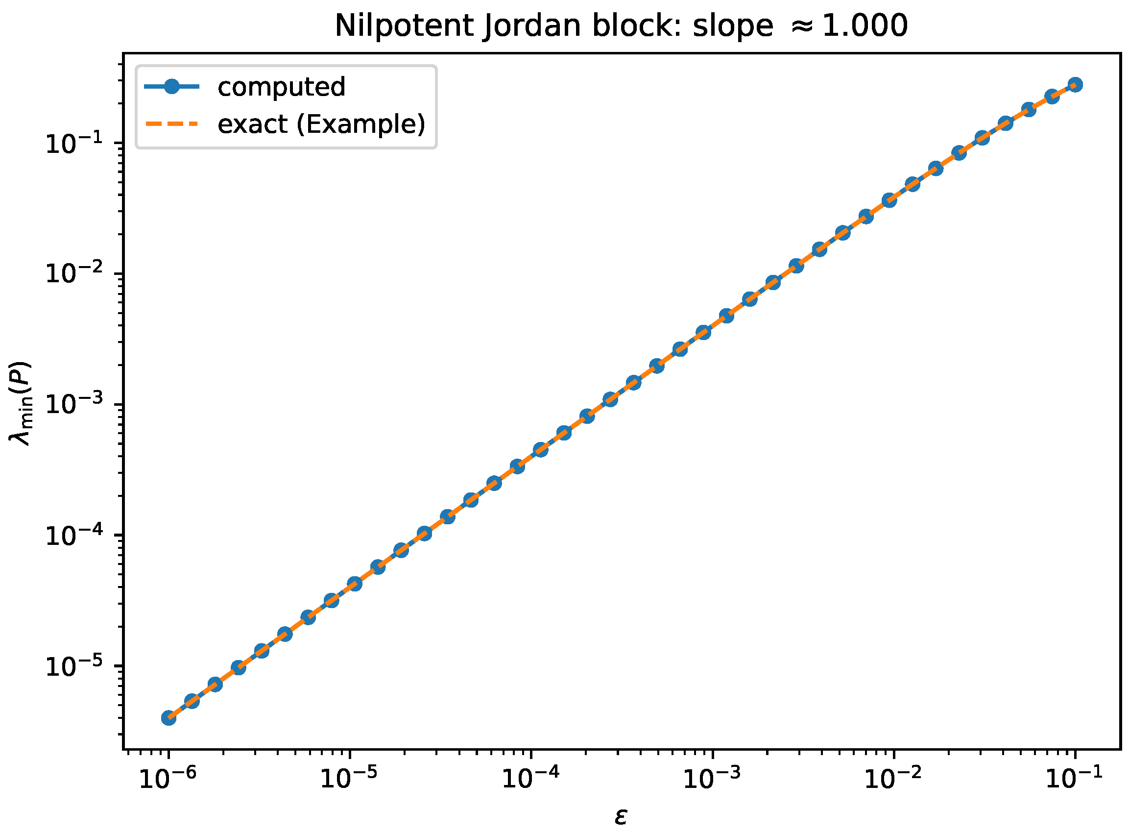
- Experiment 1: exact linear rate for the nilpotent Jordan block. We revisit Example 3 with and the disk exhaustion , . Writing , one has the exact formula , hence linear degeneracy as . Figure 1 compares the computed smallest eigenvalue to the exact expression.
Figure 1.
Nilpotent Jordan block (Example 3): log–log plot of versus , illustrating the predicted linear scaling.
Figure 1.
Nilpotent Jordan block (Example 3): log–log plot of versus , illustrating the predicted linear scaling.
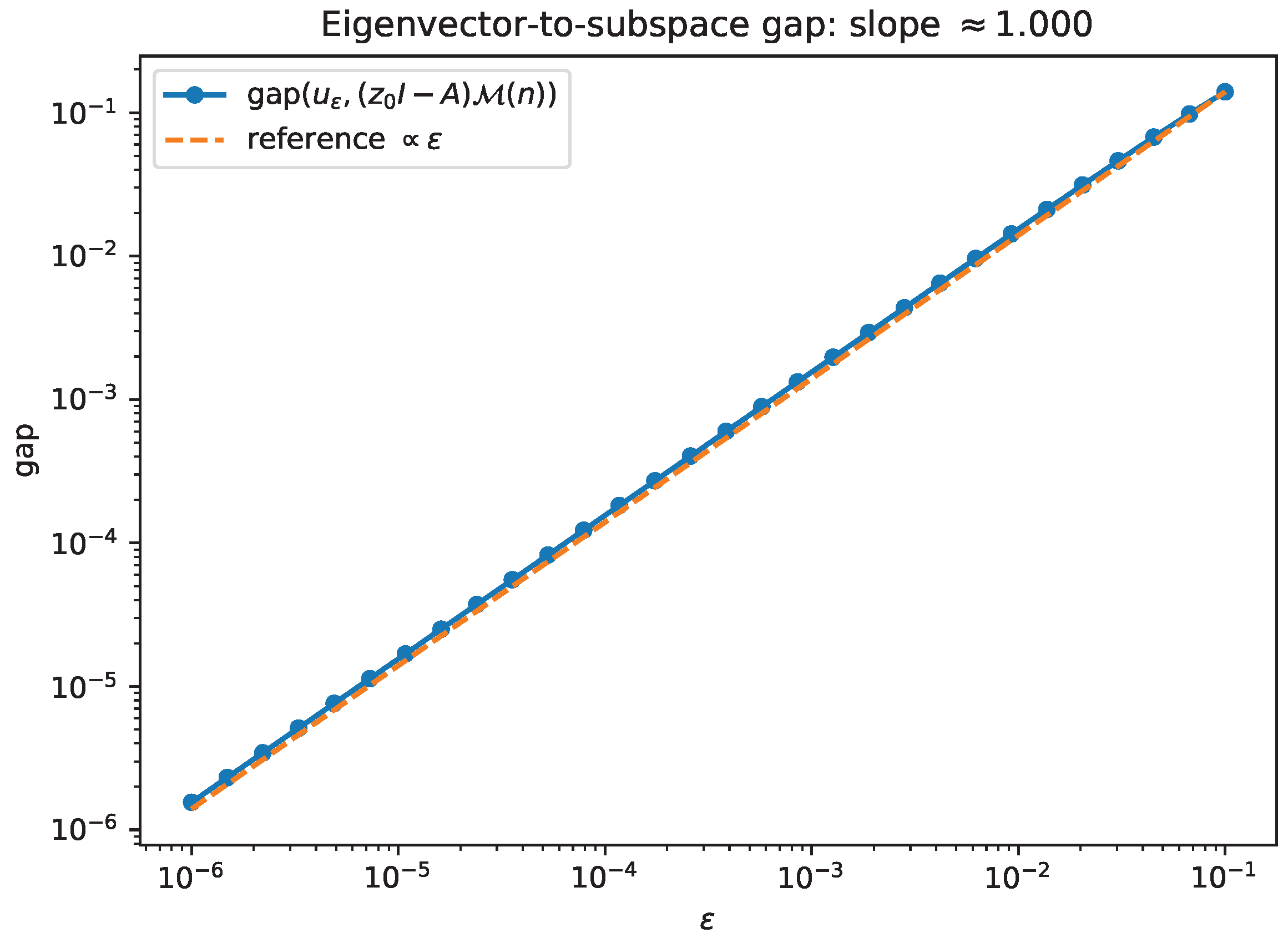
- Experiment 2: generic nonnormal matrix—linear degeneracy and eigenvector convergence. We generate a fixed random complex matrix (seeded for reproducibility), fix one direction , and form as above. Figure 2 shows against on a log–log scale, together with a reference line; the observed slope is on the plotted range. Figure 3 tracks the distance of a min-eigenvector of to the predicted limiting subspace , quantified by where is the orthogonal projector onto (consistent with Theorem 1).
Figure 2.
Random nonnormal (fixed seed) and fixed direction n: scales linearly with (Corollary 3).
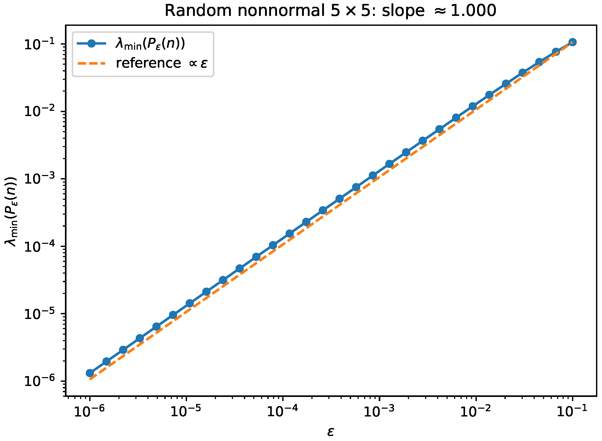
Figure 3.
Same setup as Figure 2: the direction of a min-eigenvector converges to as (Theorem 1). The plotted “gap” is .
Figure 3.
Same setup as Figure 2: the direction of a min-eigenvector converges to as (Theorem 1). The plotted “gap” is .
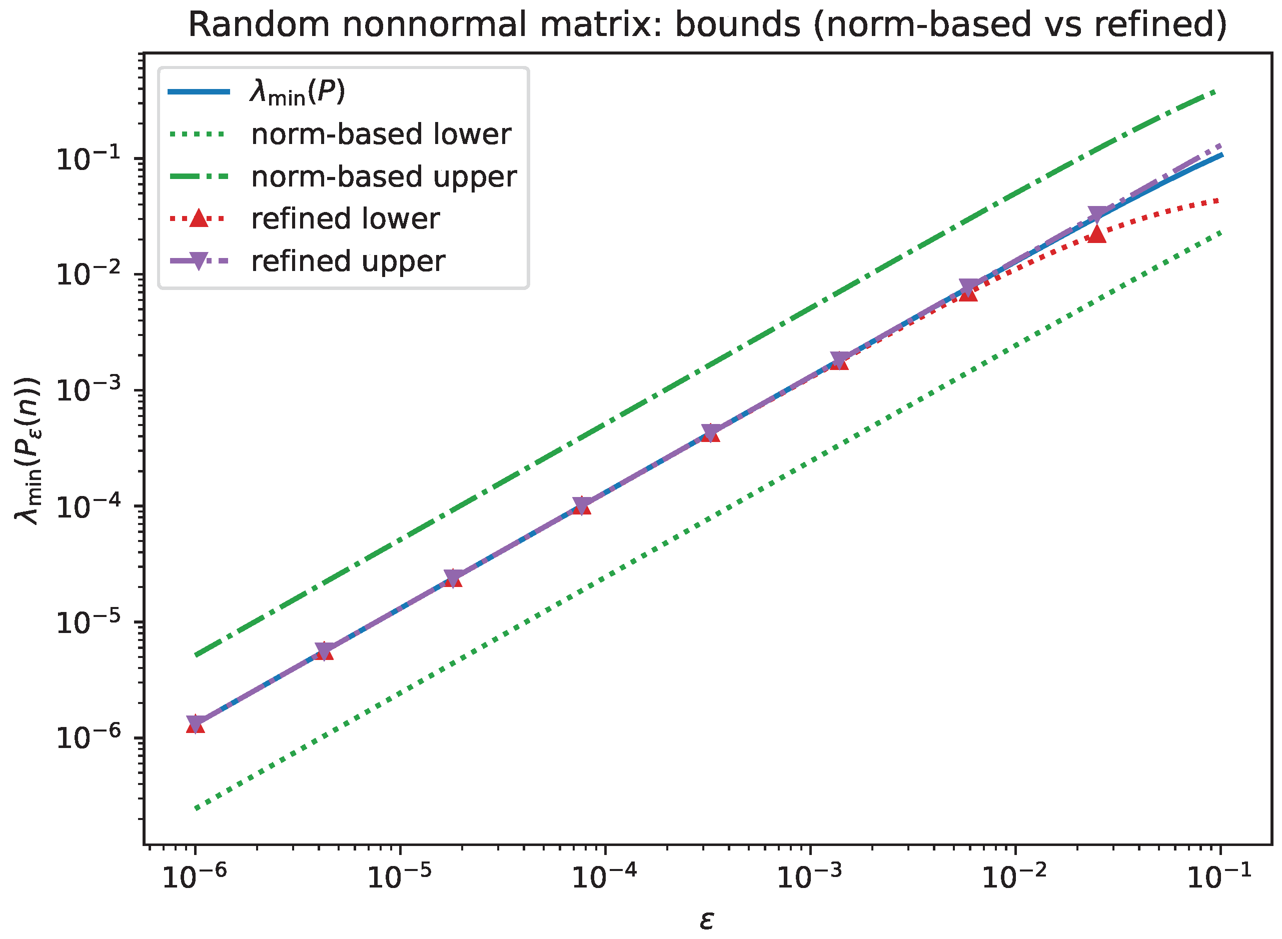
- Experiment 2b: local sharpness of norm-based versus refined bounds. We compare the norm-based bounds from Lemma 3 (c) with the refined bounds of Proposition 5. For the Jordan block, Figure 4 shows that the refined bounds track the exact eigenvalue closely and are asymptotically sharp, while the norm-based upper bound is typically much looser. For the random nonnormal matrix, Figure 5 shows the same qualitative behavior.
Figure 4.
Nilpotent Jordan block: comparison of with the norm-based bounds from Lemma 3 (c) and the refined bounds from Proposition 5.
Figure 4.
Nilpotent Jordan block: comparison of with the norm-based bounds from Lemma 3 (c) and the refined bounds from Proposition 5.
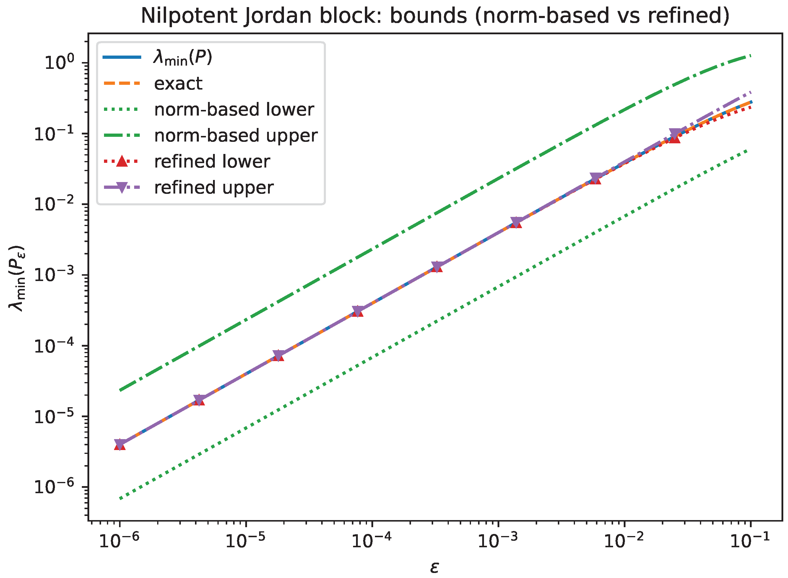
Figure 5.
Random nonnormal , fixed direction n: comparison of with the norm-based and refined bounds. The refined bounds recover the correct first-order constant as .
Figure 5.
Random nonnormal , fixed direction n: comparison of with the norm-based and refined bounds. The refined bounds recover the correct first-order constant as .
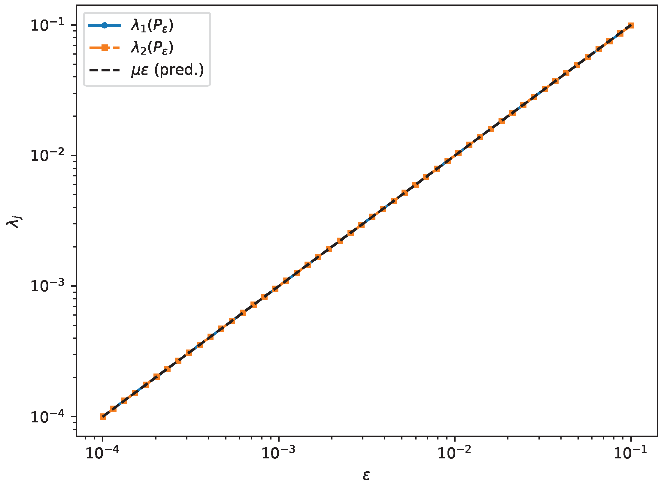
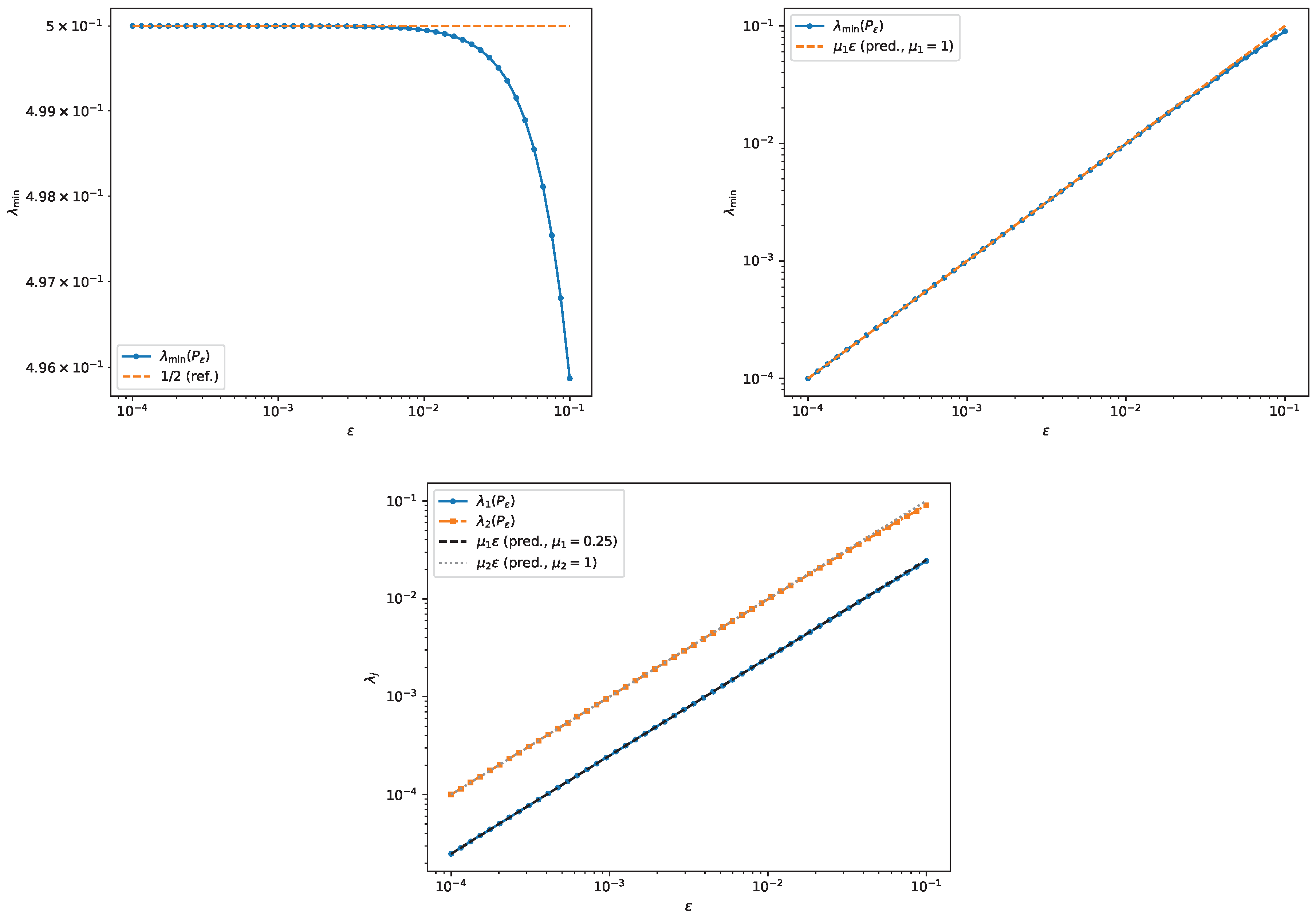
- Experiment 2c: full slope spectrum at a flat face (). Proposition 7 predicts a two-dimensional collapsing cluster when the supporting pencil has a two-dimensional maximal eigenspace and the chosen support point lies in the interior of the corresponding face. To isolate this mechanism in a fully explicit setting, we take a normal diagonal matrixso that has with multiplicity and . With , the associated support point is , lying in the relative interior of the face joining 1 and . In this basis, restricts to on , hence and the predicted slope spectrum is . Numerically we observe and as , and the face-detector count in Corollary 5 stabilizes at .
Figure 6.
Experiment 2c: two collapsing eigenvalues and their rescaled slopes in the flat-face normal example.
Figure 6.
Experiment 2c: two collapsing eigenvalues and their rescaled slopes in the flat-face normal example.
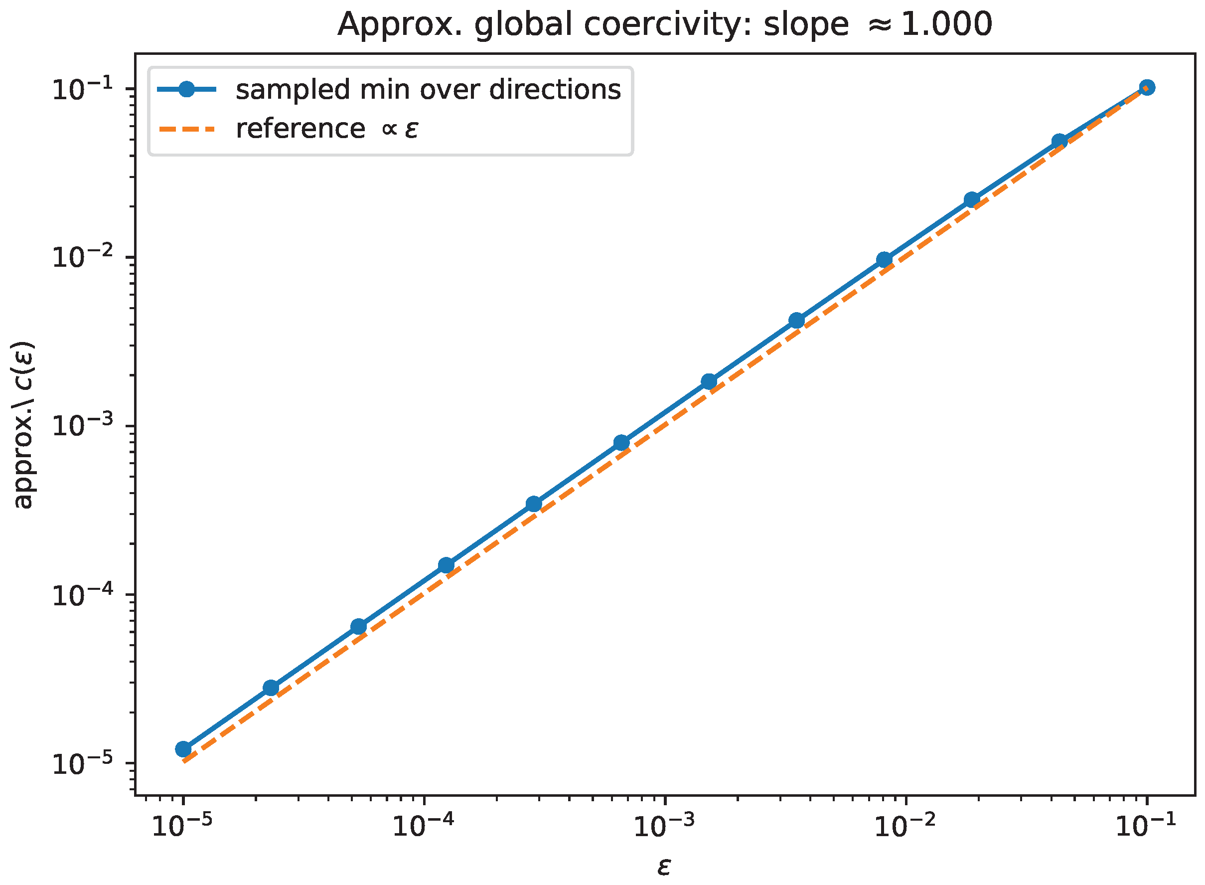
- Experiment 3: approximate global coercivity collapse. For the same random nonnormal matrix A as in Experiment 2, we approximate the global coercivity constantby sampling a fine grid of directions and using the offset model . Figure 7 plots the sampled minimum versus , illustrating the collapse asserted by Corollary 2. (Here the offset model has , so Corollary 1 also predicts that uniform coercivity cannot persist as .)
Figure 7.
Approximate global coercivity constant computed by sampling directions and using the offset model . The sampled minimum tends to 0 as (Corollary 2).
Figure 7.
Approximate global coercivity constant computed by sampling directions and using the offset model . The sampled minimum tends to 0 as (Corollary 2).
- Experiment 3b: local slope profile across directions. For the same random nonnormal matrix and the offset model, Corollary 4 predicts the local first-order constant as . Figure 8 compares the empirically observed slope at a small fixed to the prediction across directions , while Figure 9 plots the relative error.
Figure 8.
Random nonnormal matrix: direction-wise comparison of the empirical slope with the predicted limit (Corollary 4).
Figure 8.
Random nonnormal matrix: direction-wise comparison of the empirical slope with the predicted limit (Corollary 4).
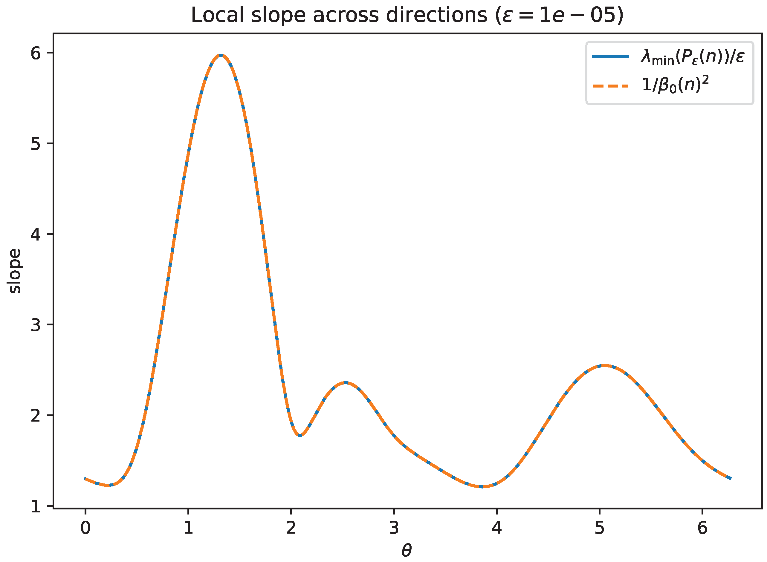
Figure 9.
Random nonnormal matrix: relative error of the prediction in Figure 8. The error decreases as the test value of is reduced.
Figure 9.
Random nonnormal matrix: relative error of the prediction in Figure 8. The error decreases as the test value of is reduced.
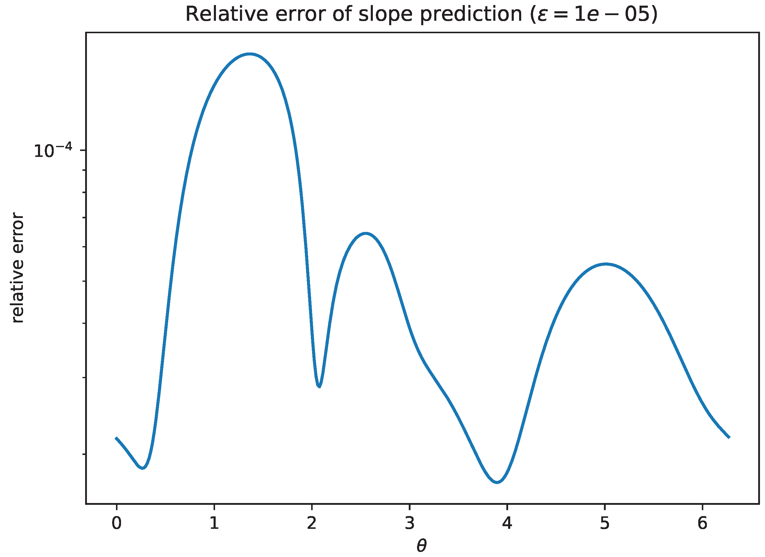
Figure 10.
Random nonnormal matrix: profile of . The global slope constant is set by the maximum of this profile (Proposition 6).
Figure 10.
Random nonnormal matrix: profile of . The global slope constant is set by the maximum of this profile (Proposition 6).
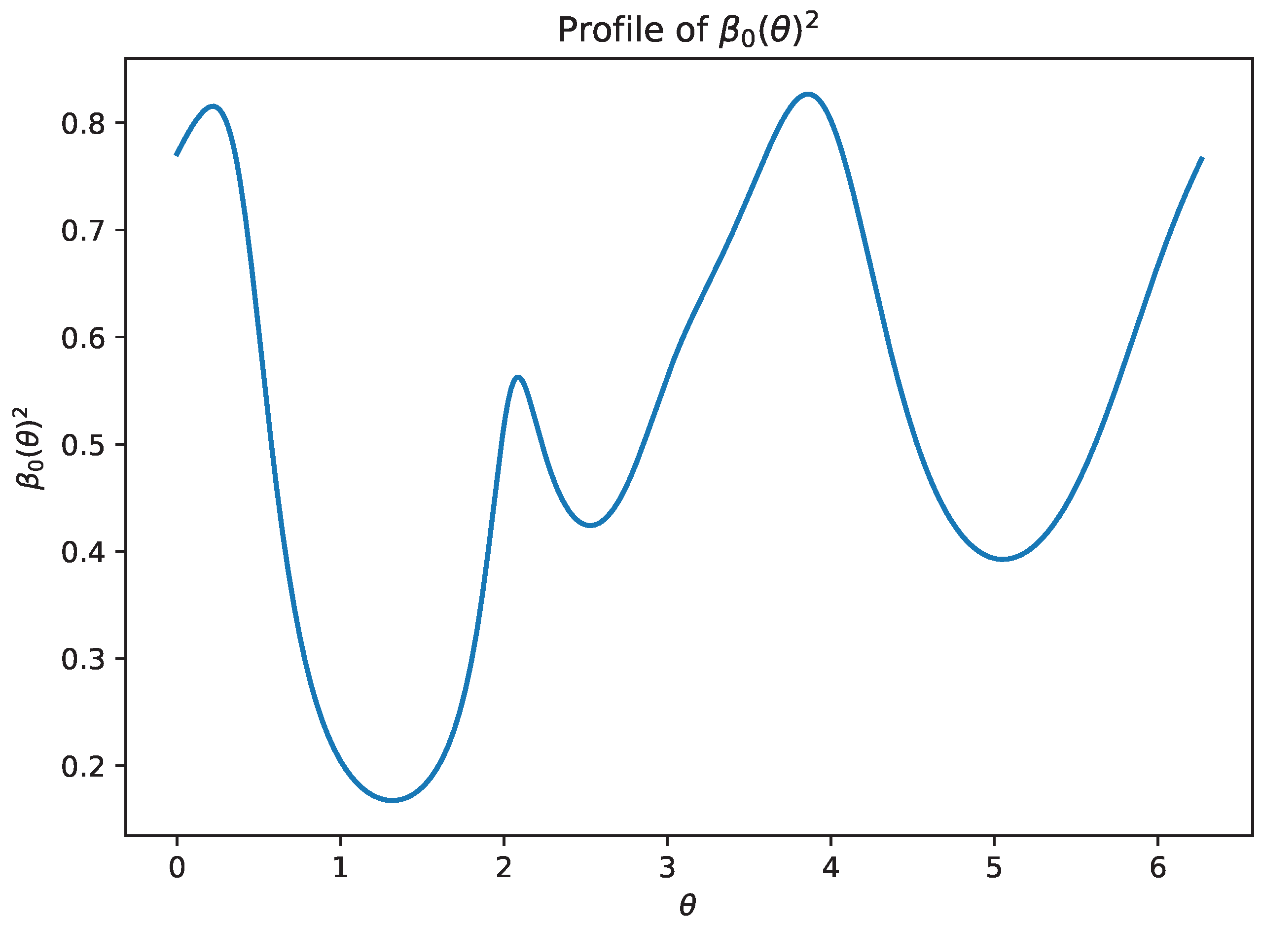
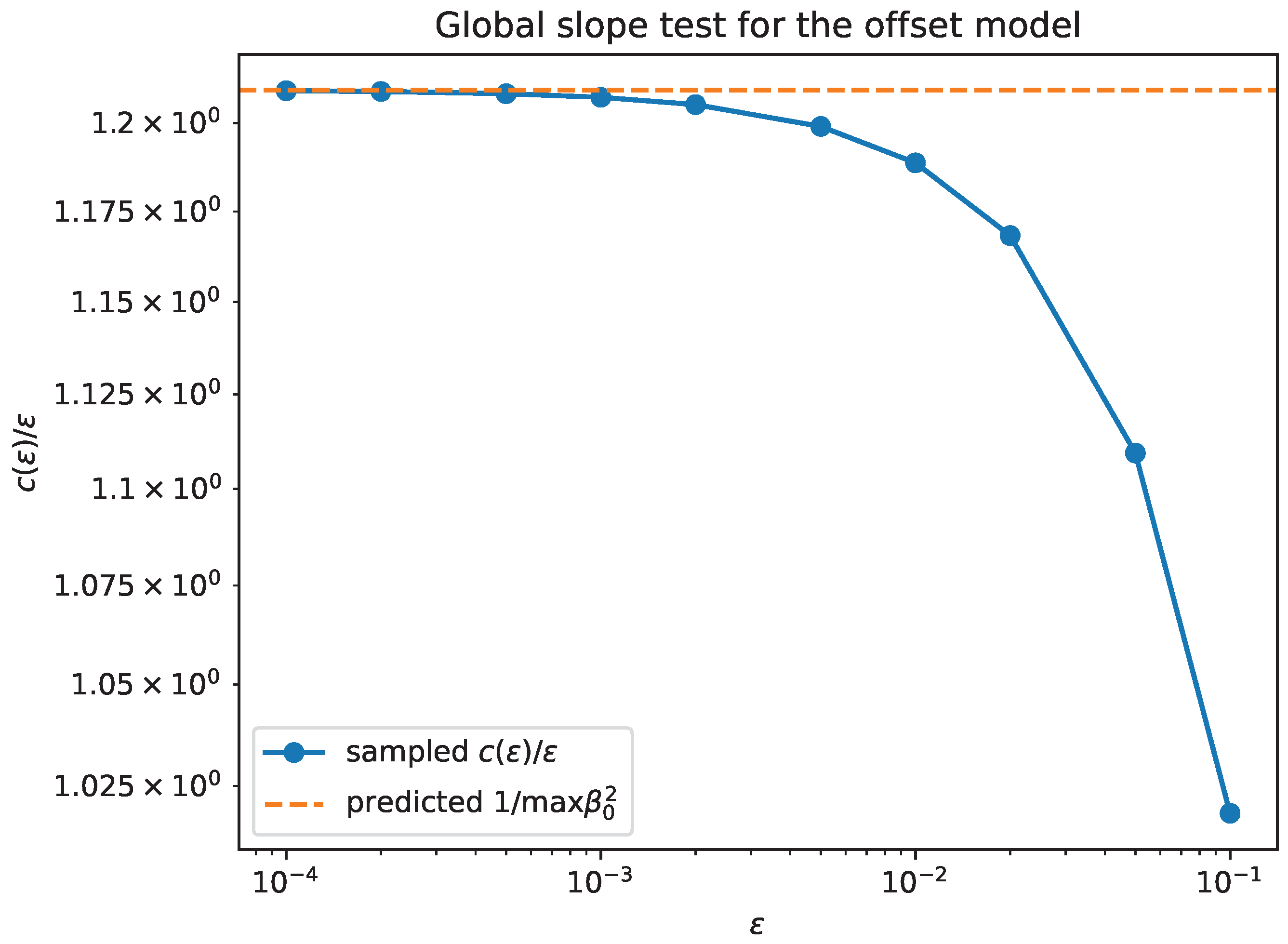
Figure 11.
Random nonnormal matrix: the sampled ratio versus , together with the predicted limit (Proposition 6).
Figure 11.
Random nonnormal matrix: the sampled ratio versus , together with the predicted limit (Proposition 6).
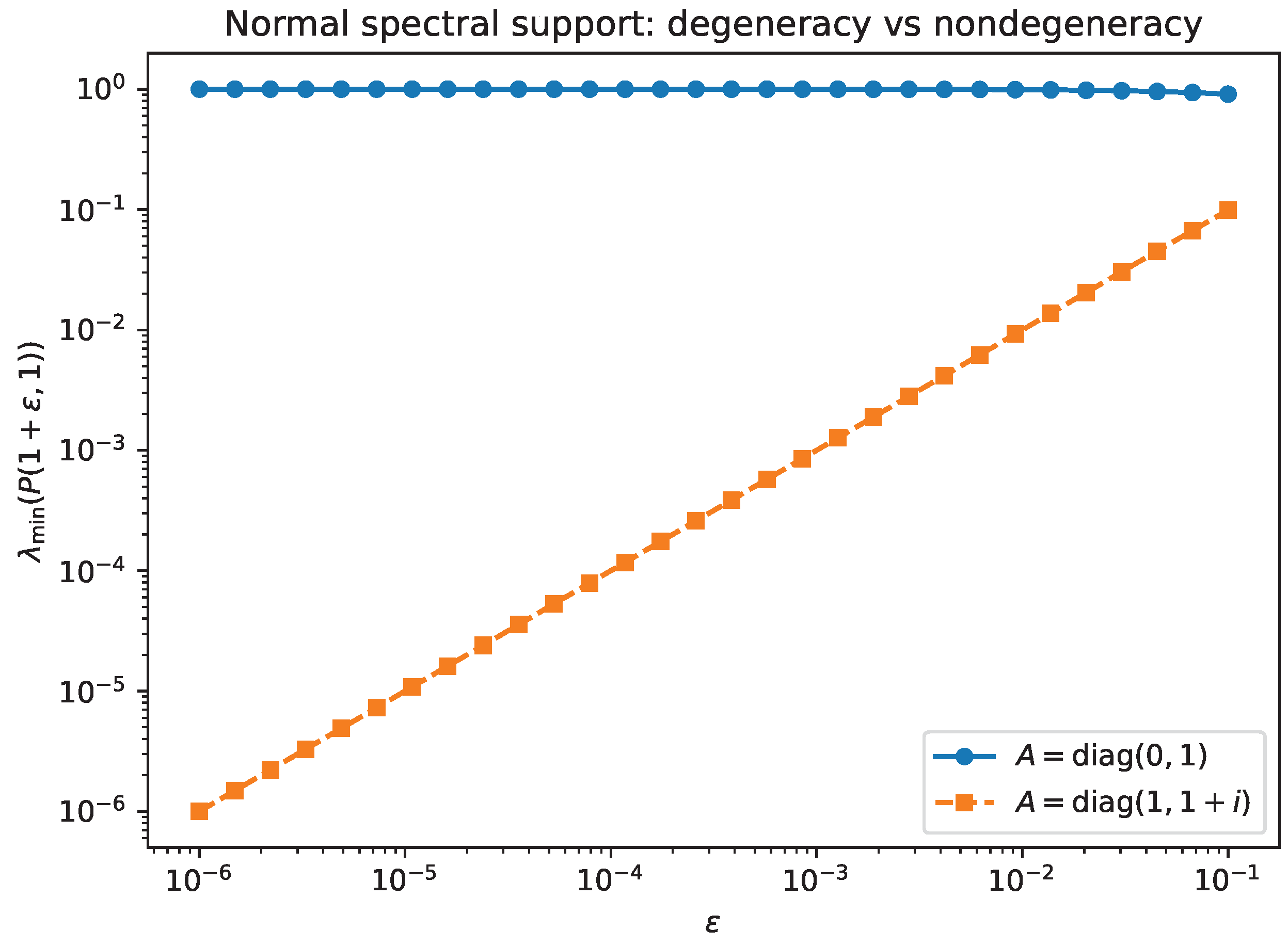
- Experiment 4: normal matrices at spectral support points. We reproduce the contrasting behavior in Examples 1–2 by evaluating for two diagonal (hence normal) matrices: and . Figure 12 shows that the former remains bounded away from 0 as , while the latter degenerates linearly, consistent with Proposition 11.
Figure 12.
Normal matrices at a spectral support point: remains bounded away from 0, whereas degenerates linearly, consistent with Proposition 11.
Figure 12.
Normal matrices at a spectral support point: remains bounded away from 0, whereas degenerates linearly, consistent with Proposition 11.
-
Experiment 4b: three-scale splitting at spectral support points (nonnormal). Proposition 12 predicts a three-scale structure at under non-tangential offsets : an exact blow-up on the geometric eigenspace , an collapsing cluster of dimension on , and an bulk bounded away from 0. We test this on three small nonnormal examples with and :
- (SS1)
- , for which (blow-up only; no cluster);
- (SS2)
- , for which and (one collapsing slope);
- (SS3)
- with and , , for which and (two collapsing slopes).
In each case we observe the predicted behavior: the largest eigenvalue scales as , the smallest eigenvalues scale linearly in with slopes given by , and the next eigenvalue remains separated from 0 uniformly in .
- Reproducibility. All figures are generated by the accompanying scripts poisson_utils.py and run_numerical_experiments.py, which require only NumPy and Matplotlib and save PDF figures into a figs/ folder.
Figure 13.
Experiment 4b: three-scale splitting at spectral support points (SS0–SS2). Each panel shows the blow-up eigenvalue(s), the collapsing cluster, and the bulk.
Figure 13.
Experiment 4b: three-scale splitting at spectral support points (SS0–SS2). Each panel shows the blow-up eigenvalue(s), the collapsing cluster, and the bulk.
4.10. A Curvature Surrogate Question at Smooth Exposed Points
The direction-dependent slope data in Corollary 4 and Proposition 7 suggest that the rescaled Poisson degeneracy rate can be viewed as a quantitative “stiffness” of the numerical range boundary in a given direction.
Let and consider the support function
where . At directions where the maximal eigenvalue is simple, choose the corresponding unit eigenvector and set the exposed support point
For the non-tangential offset family , define . When , Proposition 7 gives the explicit slope
A natural question is how compares to geometric curvature data of . In convex geometry, the support function determines the boundary, and for strictly convex curves the radius of curvature can be expressed in terms of h and its second derivative (see, e.g., [12]). For numerical ranges, is an algebraic curve determined by the Kippenhahn polynomial [14], with corners and flat portions corresponding to eigenvalue multiplicities and supporting-face degeneracies.
Question. At smooth exposed boundary points where , is the slope in (4.37) comparable (in an appropriate quantitative sense) to the curvature (or radius of curvature) of at ? Numerically, plots of (Experiment 3b) show sharp spikes near directions associated with nearly-flat faces, suggesting that may serve as an easily computable curvature surrogate.
4.11. Discussion and Remaining Open Problems
Remark 9
(Beyond the geometric three-scale picture). The bounded-resolvent regime is treated in Theorem 1 and quantified by the slope spectra in Section 4.4. At spectral support points , Proposition 11 and Corollary 7 give a complete normal-matrix description, and Proposition 12 provides a three-scale splitting for general matrices under a gap hypothesis for the supporting pencil .
Several aspects of the nonnormal spectral-support regime remain open:
- (i)
- Defective eigenvalues. When has nontrivial Jordan chains, generalized eigenvectors may exhibit higher-order resolvent blow-up (typically for a length-p Jordan block). A systematic description of how Jordan structure and the support pencil interact to determine the full singular-value/eigenvalue profile of is closely related to pseudospectral growth; see [13].
- (ii)
- Tangential approach geometry. Our slope spectra are derived for non-tangential offsets and for general exhaustions after normalization by the scalar support gap δ. Understanding when the scaling persists under more tangential approach, or when higher-order scalings appear, is largely open.
- (iii)
- Loss of spectral isolation. The explicit slope spectra rely on a gap separating from the rest of the spectrum. When this gap closes, the associated projectors become ill-conditioned and new multi-scale behaviors may appear.
References
- O. Toeplitz, Das algebraische Analogon zu einem Satze von Fejér, Math. Z. 2 (1918), no. 1–2, 187–197. [CrossRef]
- F. Hausdorff, Der Wertevorrat einer Bilinearform, Math. Z. 3 (1919), no. 1, 314–316. [CrossRef]
- M. Crouzeix, Bounds for analytical functions of matrices, Integr. Equ. Oper. Theory 48 (2004), 461–477. [CrossRef]
- M. Crouzeix, Numerical range and functional calculus in Hilbert space, J. Funct. Anal. 244 (2007), no. 2, 668–690. [CrossRef]
- M. Crouzeix and C. Palencia, The numerical range is a (1+√2)-spectral set, SIAM J. Matrix Anal. Appl. 38 (2017), no. 2, 649–655. [CrossRef]
- B. Delyon and F. Delyon, Generalization of von Neumann’s spectral sets and integral representation of operators, Bull. Soc. Math. France 127 (1999), no. 1, 25–41. [CrossRef]
- C. Badea, M. Crouzeix, and B. Delyon, Convex domains and K-spectral sets, Math. Z. 252 (2006), no. 2, 345–365. [CrossRef]
- F. L. Schwenninger and J. de Vries, The double-layer potential for spectral constants revisited, Integr. Equ. Oper. Theory 97 (2025), 13. [CrossRef]
- M. Crouzeix and A. Greenbaum, Spectral Sets: Numerical Range and Beyond, SIAM J. Matrix Anal. Appl. 40 (2019), no. 3, 1087–1101. [CrossRef]
- T. Kato, Perturbation Theory for Linear Operators, 2nd ed., Classics in Mathematics, Springer, 1995. [CrossRef]
- C. Davis and W. M. Kahan, The rotation of eigenvectors by a perturbation. III, SIAM J. Numer. Anal. 7 (1970), 1–46. [CrossRef]
- R. Schneider, Convex Bodies: The Brunn–Minkowski Theory, 2nd ed., Encyclopedia of Mathematics and its Applications, Cambridge University Press, 2014. [CrossRef]
- L. N. Trefethen and M. Embree, Spectra and Pseudospectra: The Behavior of Nonnormal Matrices and Operators, Princeton University Press, 2005. [CrossRef]
- R. Kippenhahn, Über den Wertevorrat einer Matrix, Math. Nachr. 6 (1951), 193–228. [CrossRef]
Disclaimer/Publisher’s Note: The statements, opinions and data contained in all publications are solely those of the individual author(s) and contributor(s) and not of MDPI and/or the editor(s). MDPI and/or the editor(s) disclaim responsibility for any injury to people or property resulting from any ideas, methods, instructions or products referred to in the content. |
© 2026 by the authors. Licensee MDPI, Basel, Switzerland. This article is an open access article distributed under the terms and conditions of the Creative Commons Attribution (CC BY) license (http://creativecommons.org/licenses/by/4.0/).
Copyright: This open access article is published under a Creative Commons CC BY 4.0 license, which permit the free download, distribution, and reuse, provided that the author and preprint are cited in any reuse.


