Differentially Constrained Manifolds for Data-Efficient ECG Classification

1. Introduction

1.1. Problem and Importance

ECG beat classification is a clinically relevant pattern recognition task [1,2], but in many realistic settings labeled data are limited, expensive to curate, and unevenly distributed across rhythm types. In the small data regime, a model can overfit to idiosyncratic morphology, learn unstable decision boundaries, and fail to generalize across records and patients. This motivates methods that improve sample efficiency by constructing useful additional training signal and by selecting training subsets that preserve information content. The problem setting in this work has two coupled goals. First, generate augmented samples that preserve local geometry of the underlying signal rather than injecting arbitrary noise. Second, train accurate models using limited training budgets by selecting or weighting samples that remain stable under structure preserving perturbations.

1.2. What Problems This Solves

The methodology targets the following practical issues.

• Label scarcity and small training budgets. Improve test accuracy when only a small subset of beats can be used for training.
• Overfitting to unstable examples. Identify samples whose predictions degrade sharply under structured perturbations and reduce their influence during training.
• Unrealistic augmentation artifacts. Replace generic noise based augmentation with curvature governed parabolic jumps that are local, smooth, and naturally stabilizing [3,4,5].
• Reproducibility. Provide a deterministic evaluation pipeline under fixed dataset files and fixed seeds.

1.3. Literature Review

Regression and supervised learning baselines.

Regression remains a foundational supervised learning tool, both directly for prediction and indirectly as a building block for regularization, feature selection, and stability analysis. Classical regularized regression methods include ridge regression [6], the lasso [7], and the elastic net [8], all of which are highly cited and widely used as baselines for high dimensional learning. Tree based regression and classification methods such as random forests [9] and gradient boosting [10] provide strong supervised baselines and are frequently competitive on tabular feature representations. Modern scalable boosting systems such as XGBoost [11] further improve performance and have become standard in practice.

Unsupervised learning, manifolds, and representation learning.

Unsupervised learning methods often aim to capture low dimensional structure in high dimensional signals, using approaches such as clustering and latent variable modeling. The EM algorithm [12] is a classic framework for fitting models with latent variables. Dimensionality reduction and manifold oriented views of data are commonly connected to principal component ideas and representation learning, with neural autoencoders serving as a practical nonlinear alternative [13]. These ideas motivate treating ECG signals as lying near structured sets rather than being arbitrary vectors [14,15,16,17].

Deep learning for ECG.

Convolutional networks have achieved strong ECG classification performance at scale, including work that reports cardiologist level performance on large single lead datasets [1]. In smaller curated benchmarks, careful normalization, architecture choice, and evaluation design remain crucial [18,19,20]. The MIT BIH Arrhythmia Database is a standard reference dataset for arrhythmia research [2,21] and motivates reproducible experimental protocols.

1.4. Contributions and Organization

This paper presents a structured methodology that couples geometry guided parabolic augmentation with expression constrained perturbations and stabili4ty aware subset training. Section 2 gives preliminaries. Section 3 describes the full methodology, separated into supervised and unsupervised components and anchored to widely used regression baselines. Section 4 organizes the innovation in methodology by consolidating the geometric augmentation and expression constrained manifold components that were outlined in the working document. Section 5 explores some properties and theorems related to differentially constrained manifolds. Section 6 introduces the case study on the MIT BIH Arrythmia Database. Section 7 gives a conclusion on the theory and the experiment on the Arrythmia Database. An appendix section is included with the GitHub link to the experiment’s code.

2. Preliminaries

2.1. Linear Algebra

We use standard linear algebra concepts for vectors, norms, inner products, projections, and matrix decompositions as background, following the style of Lipschutz. These tools appear implicitly in minimal norm solutions, feature normalization, and embedding based classification.

2.2. Statistics

We assume familiarity with random variables, expectations, sampling, and basic distributions. In particular, we use distributional modeling of positive spacings via exponential and Gamma variables to control reciprocal terms and avoid instability near zero.

2.3. Deep Learning with Python and Python

All models and algorithms are implemented in Python, with deep learning components implemented using standard GPU accelerated workflows [22]. We assume familiarity with dataset pipelines, optimization with gradient descent variants, and evaluation under deterministic seeds.

3. Methodology

3.1. Overview

The methodology is a discovered methodology that exists as a combined pipeline, not a claim of a new learning paradigm. It combines:

• curvature and gravity guided parabolic jump augmentation in the signal domain
• learned class specific expression constraints used to generate structure preserving perturbations
• supervised stability scoring using margin drop under perturbations
• unsupervised diversity sampling in feature space
• deterministic subset training comparisons at fixed budgets

3.2. Supervised Component

3.2.1. Problem Formulation

Let $w\in {\mathbb{R}}^{256}$ be an ECG beat window and $y\in \{0,1,2\}$ its label. A model $f_{\theta }$ produces logits $\ell \in {\mathbb{R}}^3$ and is trained with cross entropy. The primary supervised objective is accurate generalization on a held out test set under limited training budgets.

3.2.2. Regression Baselines and the Role of Highly Cited Regression Methods

To ground evaluation in standard supervised learning, the methodology is compatible with classical regression and regularization baselines that are widely cited.

• Ridge regression [6] as a baseline for stable linear prediction under collinearity.
• The lasso [7] for sparse feature selection and interpretable linear models.
• Elastic net [8] combining shrinkage and selection in correlated feature settings.
• Random forests [9] and gradient boosting [10] for strong supervised prediction on engineered features.
• XGBoost [11] as a scalable and competitive boosted tree baseline.

These methods serve two roles: first as performance baselines on feature vectors $\varphi \left(w\right)$, and second as conceptual anchors for stability via regularization and margin behavior.

3.2.3. Classifier Used in This Work

The primary model is a 1D residual convolutional encoder producing a normalized embedding $z\in {\mathbb{R}}^{128}$ and a linear head $\ell =Wz+b$. This follows the working document description and is trained using cross entropy.

3.2.4. Supervised Stability Scoring via Margin Drop

Given logits ℓ and true class c, define the margin

$$\mathrm{margin}(\ell ,c)={\ell }_c-\underset{j\ne c}{max}{\ell }_j.$$

For each beat, generate multiple constraint respecting perturbations and compute nonnegative margin drops. Aggregate using the mean of the top $25\%$ largest drops to obtain $\mathrm{MD}\left(w\right)$. This produces a supervised stability score because it depends on model predictions and labels through the margin definition [23,24].

3.2.5. Weighted Training

Given $\mathrm{MD}\left(w_i\right)$ for selected training beats, define weights

$${\omega }_i=max(0.05,e^{-\lambda \mathrm{MD}\left(w_i\right)}).$$

Train with weighted cross entropy. This emphasizes stable samples under the learned expression perturbations and can improve generalization in small budget settings.

3.3. Unsupervised Component

3.3.1. Feature Based Diversity Selection

Each beat is mapped to a hand crafted feature vector $\varphi \left(w\right)$ consisting of basic statistics, downsampled waveform and derivative, and a short FFT magnitude summary, then normalized. Within each class, farthest point sampling selects points that maximize coverage in feature space. This step is unsupervised in the sense that it operates on geometry in feature space and does not require gradients or a learned model, although it may be performed within class partitions.

3.3.2. Expression Constrained Perturbations as Manifold Projections

For each class c, a learned expression of the form

$${a\left|x\right|}^m{\left|p\right|}^n+{b\left|y\right|}^k{\left|q\right|}^r\approx 1$$

defines an implicit constraint set. The perturbation operator iteratively modifies a beat to reduce constraint residual while respecting curvature and amplitude caps and preserving the QRS region. This behaves like a projection toward a class specific structured set, aligning with common unsupervised views of signals as lying near manifolds or low dimensional sets, and conceptually connects to representation and denoising ideas [13].

3.3.3. Latent Variable Viewpoint

The iterative projection can also be interpreted through a latent variable lens, where an unobserved structured representation is inferred from an observed signal via repeated updates. This viewpoint is broadly compatible with classic incomplete data optimization frameworks such as EM [12].

4. Innovation in Methodology

This section reorganizes the existing outline and removes redundancy while keeping the exact technical content already written.

4.1. Problem Setting

We are given a discrete dataset of points

$${\left\{(x_i,y_i)\right\}}_{i=0}^N\subset {\mathbb{R}}^2,$$

with strictly increasing $x_i$. The goal is data augmentation: to generate additional points between or beyond existing points while preserving the geometric structure of the data.

The augmentation must:

• be local,
• respect the second order structure of the data,
• allow extrapolation beyond existing points,
• stabilize naturally after a few iterations,
• and produce smooth, realistic trajectories.

4.2. Discrete Differences, Curvature Strength, and Gravity

Define first differences

$$\Delta x_i=x_{i+1}-x_i,\Delta y_i=y_{i+1}-y_i.$$

Define the discrete second difference of y with respect to x by

$$A_i\approx {\displaystyle \frac{\Delta y_{i+1}-\Delta y_i}{{(\Delta x_i)}^2}}.$$

We define a scalar field $g_i$, called gravity, by

$$g_i={\displaystyle \frac{1}{|A_i|+\epsilon }},$$

where $\epsilon >0$ is a small stabilizing constant. Interpretation:

• Large curvature implies $|A_i|$ large implies $g_i$ small.
• Small curvature implies $|A_i|$ small implies $g_i$ large.

Thus $g_i$ acts as an inverse curvature stiffness and directly modulates the strength of augmentation.

4.3. Local Chord Geometry and Parabolic Deviation Magnitude

Define the slope of the chord connecting endpoints:

$$m_i={\displaystyle \frac{y_{i+1}-y_i}{x_{i+1}-x_i}}.$$

The factor

$${\displaystyle \frac{1}{\sqrt{1+m_i^2}}}$$

projects vertical deviation onto the normal direction of the chord.

Each augmentation step is modeled as a local parabolic jump. A classical geometric result states that the maximum distance between a parabola

$$y=A_i{x}^2+Bx+C$$

and its chord over an interval of width $\Delta x_i$ occurs at the midpoint and equals

$$b_i={\displaystyle \frac{|A_i|}{\sqrt{1+m_i^2}}}{\displaystyle \frac{{(\Delta x_i)}^2}{4}}.$$

Using the definition of $g_i$, this can be written equivalently as

$$b_i={\displaystyle \frac{1}{g_i}}{\displaystyle \frac{{(\Delta x_i)}^2}{4\sqrt{1+m_i^2}}}.$$

This quantity represents the normal displacement of the parabolic jump.

4.4. Augmented Point Construction Including the x Direction

Let $s_i$ be the scaling factor produced by the chosen differential expression analysis, typically near 1, and let it saturate via

$${\tilde{s}}_i=\mathrm{clip}(s_i,s_{min},s_{max}).$$

Define the augmented horizontal displacement

$$\Delta X_i={\tilde{s}}_i\Delta x_i,x_i^{\mathrm{new}}=x_i+\Delta X_i.$$

Define the chord slope

$$m_i={\displaystyle \frac{\Delta y_i}{\Delta x_i}}.$$

Using the parabolic deviation bound, the normal (vertical) deviation magnitude is

$$b_i={\displaystyle \frac{|A_i|}{\sqrt{1+m_i^2}}}{\displaystyle \frac{{(\Delta X_i)}^2}{4}}={\displaystyle \frac{1}{g_i}}{\displaystyle \frac{{(\Delta X_i)}^2}{4\sqrt{1+m_i^2}}},{\sigma }_i=\mathrm{sign}\left(A_i\right).$$

Then the augmented y value is

$$y_i^{\mathrm{new}}=y_i+{\sigma }_i{b}_i.$$

Hence the augmented point is

$$(x_i^{\mathrm{new}},y_i^{\mathrm{new}})=\left(x_i+\Delta X_i,y_i+{\sigma }_i{b}_i\right),$$

and overshoot beyond $(x_{i+1},y_{i+1})$ is allowed whenever ${\tilde{s}}_i>1$.

4.5. Iterative Refinement and Stabilization

To refine augmented values, an iterative update may be used. At iteration k, treat x as unknown and solve

$$\mathrm{\Phi }(x^{(k+1)},y^{\left(k\right)},p^{\left(k\right)},q^{\left(k\right)})=1,$$

then treat p as unknown and solve

$$\mathrm{\Phi }(x^{(k+1)},y^{(k+1)},p^{(k+1)},q^{\left(k\right)})=1.$$

Stabilization is achieved via blending:

$$x^{(k+1)}\leftarrow (1-\alpha )x^{\left(k\right)}+\alpha x^{(k+1)},p^{(k+1)}\leftarrow (1-\alpha )p^{\left(k\right)}+\alpha p^{(k+1)}.$$

Iterations stop naturally when updates become negligible, or when $A_i$ (hence $g_i$) stabilizes.

4.6. Why the Jumps Are Parabolic

In local coordinates aligned with the chord:

• tangential displacement scales linearly with $\Delta x_i$,
• normal displacement scales quadratically with $\Delta x_i$.

Thus the augmentation satisfies

$$\mathrm{normal}\mathrm{displacement}\propto {\left(\tan \mathrm{gential}\mathrm{displacement}\right)}^2,$$

which is precisely the defining property of a parabola. This corresponds to the second order osculating parabola expansion of a curve in differential geometry.

4.7. Movement Regulation Function and Scaling Factor Definition

We define the movement regulation function

$$F(x,y,p,q)=1,F(x,y,p,q):=3x^{2}p+yq.$$

For a fixed $(x,y)$, this equation defines a one parameter family of admissible $(p,q)$. To obtain a unique and stable value, we choose the minimal norm solution. The minimal norm solution of

$$3x^{2}p+yq=1$$

is

$$(p,q)={\displaystyle \frac{(3x^2,y)}{9x^4+y^2}}.$$

For each index i, a theoretical value $x_i^{\mathrm{theoretical}}$ is obtained by iteratively solving the movement regulation equation while treating all other quantities as fixed, alternating between solving for x and solving for p, until convergence. Let $x_i^{\mathrm{real}}=x_i$ denote the original data value. We define the scaling factor as

$$s_i={\displaystyle \frac{x_i^{\mathrm{theoretical}}}{x_i^{\mathrm{real}}}}.$$

To prevent runaway scaling, $s_i$ is saturated:

$${\tilde{s}}_i=\mathrm{clip}(s_i,s_{min},s_{max}),\mathrm{clip}(u,a,b)=min(max(u,a),b).$$

4.8. ECG Pipeline Components Already Defined

We study a three class ECG beat classification problem using the MIT BIH Arrhythmia Database [2,21]. Each beat is extracted as a fixed length window of length $T=256$ around the annotated R peak and is then robust normalized. The key idea is to combine:

• a class specific learned constraint called the learned expression
• a stability score that measures how much a model’s classification confidence drops under constraint respecting perturbations
• deterministic subset sampling strategies that target diversity and stability

The learned expression family is

$${a\left|x\right|}^m{\left|p\right|}^n+{b\left|y\right|}^k{\left|q\right|}^r\approx 1,$$

with exponents chosen from $\{1,2\}$ and $(a,b)$ fit by least squares by minimizing mean squared error against target value 1 over pooled editable indices.

The stability score uses margin drop and aggregates by the mean of the top $25\%$ largest drops:

$$\mathrm{MD}\left(w\right)=\mathrm{Top}25\mathrm{Mean}\{d_1,\dots ,d_M\}.$$

Weighted training uses

$${\omega }_i=max(0.05,e^{-\lambda \mathrm{MD}\left(w_i\right)}),$$

and minimizes weighted cross entropy.

Diversity selection uses farthest point sampling on engineered features $\varphi \left(w\right)$.

All dataset splits, subset selections, and training procedures are deterministic under fixed seeds, while learned expression estimation can vary with the expression learning subset and seed.

5. Properties and Theorems of Differentially Constrained Manifolds

5.1. Constrained Manifolds in $(x,p,y,q)$

Let $x,y$ denote algebraic state variables and let $p,q$ denote auxiliary variables that encode local change or control. A differentially constrained manifold (also referred to as Differential Expression [25]) is the implicit level set

$$\mathcal{M}=\{(x,p,y,q)\in {\mathbb{R}}^4:F(x,p,y,q)=1\},$$

where F is a polynomial expression in $(x,p,y,q)$. In this paper we focus on the practically important case where F is linear in $(p,q)$:

$$F(x,p,y,q)=P(x,y)p+Q(x,y)q+R(x,y),$$

(1)

with $P,Q,R$ polynomials in $(x,y)$. The examples used throughout are special cases with $R\equiv 0$, such as

$$2x^{2}p+yq=1,3x^{5}p+2x^{2}p+yq+y^{2}q=1.$$

5.2. What It Means to Be “Near 1” and How to Measure Farness

Given a point $z=(x,p,y,q)$, define the constraint residual

$$\rho \left(z\right)=F\left(z\right)-1.$$

Saying the constraint is “near 1” means $\left|\rho \right(z\left)\right|$ is small.

A simple normalization that forces the constraint to equal 1 at the empirical mean is:

$$\overline{z}:=(\overline{x},\overline{p},\overline{y},\overline{q}),\tilde{F}\left(z\right):={\displaystyle \frac{F\left(z\right)}{F\left(\overline{z}\right)}}.$$

Then $\tilde{F}\left(\overline{z}\right)=1$ and we measure distance by $|\tilde{F}\left(z\right)-1|$.

A geometric approximation to Euclidean distance from z to the manifold $\mathcal{M}$ is obtained by linearizing F:

$$\mathrm{dist}(z,\mathcal{M})\approx {\displaystyle \frac{\left|F\right(z)-1|}{{\parallel \nabla F\left(z\right)\parallel }_2}},$$

whenever $\nabla F\left(z\right)\ne 0$ and z is sufficiently close to $\mathcal{M}$.

Projection style correction toward the manifold.

A canonical update that tries to transform data so that the constraint value moves closer to 1 is

$$z^{+}=z-\eta {\displaystyle \frac{F\left(z\right)-1}{{\parallel \nabla F\left(z\right)\parallel }_2^2}}\nabla F\left(z\right),$$

(2)

with step size $\eta >0$. To first order, this reduces the residual because it moves in the normal direction of the level set.

5.3. A Dominance Theorem for Orders of p and q from Highest Power Terms

In the linear in $(p,q)$ setting (1) with $R\equiv 0$,

$$P(x,y)p+Q(x,y)q=1,$$

the dominant growth of P in x and the dominant growth of Q in y determine the asymptotic order needed for p and q to keep the left side bounded.

Degree notation.

For a polynomial $H(x,y)$, let ${deg}_x\left(H\right)$ be the maximum exponent of x appearing in any monomial of H, and similarly ${deg}_y\left(H\right)$.

Theorem 1 

(Highest power cancellation gives the order). Assume $P,Q$ are nonzero polynomials and consider the constraint

$$P(x,y)p+Q(x,y)q=1.$$

Fix a regime where $\left|y\right|$ is bounded and $\left|x\right|\to \infty$. If $p=p(x,y)$ and $q=q(x,y)$ remain bounded in the sense that $\left|Q\right(x,y\left)q\right|$ does not grow faster than a constant as $\left|x\right|\to \infty$, then necessarily

$$p(x,y)=O\left({\displaystyle \frac{1}{{\left|x\right|}^{{deg}_x\left(P\right)}}}\right)\mathrm{as}\left|x\right|\to \infty .$$

Similarly, fixing a regime where $\left|x\right|$ is bounded and $\left|y\right|\to \infty$, if $\left|P\right(x,y\left)p\right|$ does not grow faster than a constant as $\left|y\right|\to \infty$, then

$$q(x,y)=O\left({\displaystyle \frac{1}{{\left|y\right|}^{{deg}_y\left(Q\right)}}}\right)\mathrm{as}\left|y\right|\to \infty .$$

Proof. 

Write $P(x,y)={\sum }_{i=0}^d{a}_i\left(y\right)x^i$ with $d={deg}_x\left(P\right)$ and $a_d$ 0. As $\left|x\right|\to \infty$ with $\left|y\right|$ bounded, we have $\left|P(x,y)\right|\asymp {\left|x\right|}^d$ up to a multiplicative constant depending on the bounded y range. If $\left|Q\right(x,y\left)q\right|$ stays $O\left(1\right)$, then $P(x,y)p=1-Q(x,y)q$ is also $O\left(1\right)$. Thus $p=O(1/P)$, hence $p=O\left(\right|x{|}^{-d})$. The q statement is identical with roles exchanged.    □

Example.

For

$$3x^{5}p+2x^{2}p+yq+y^{2}q=1⟺(3x^5+2x^2)p+(y+y^2)q=1,$$

we have ${deg}_x(3x^5+2x^2)=5$ and ${deg}_y(y+y^2)=2$, so Theorem 1 yields

$$p=O(1/x^5),q=O(1/y^2),$$

in the corresponding regimes.

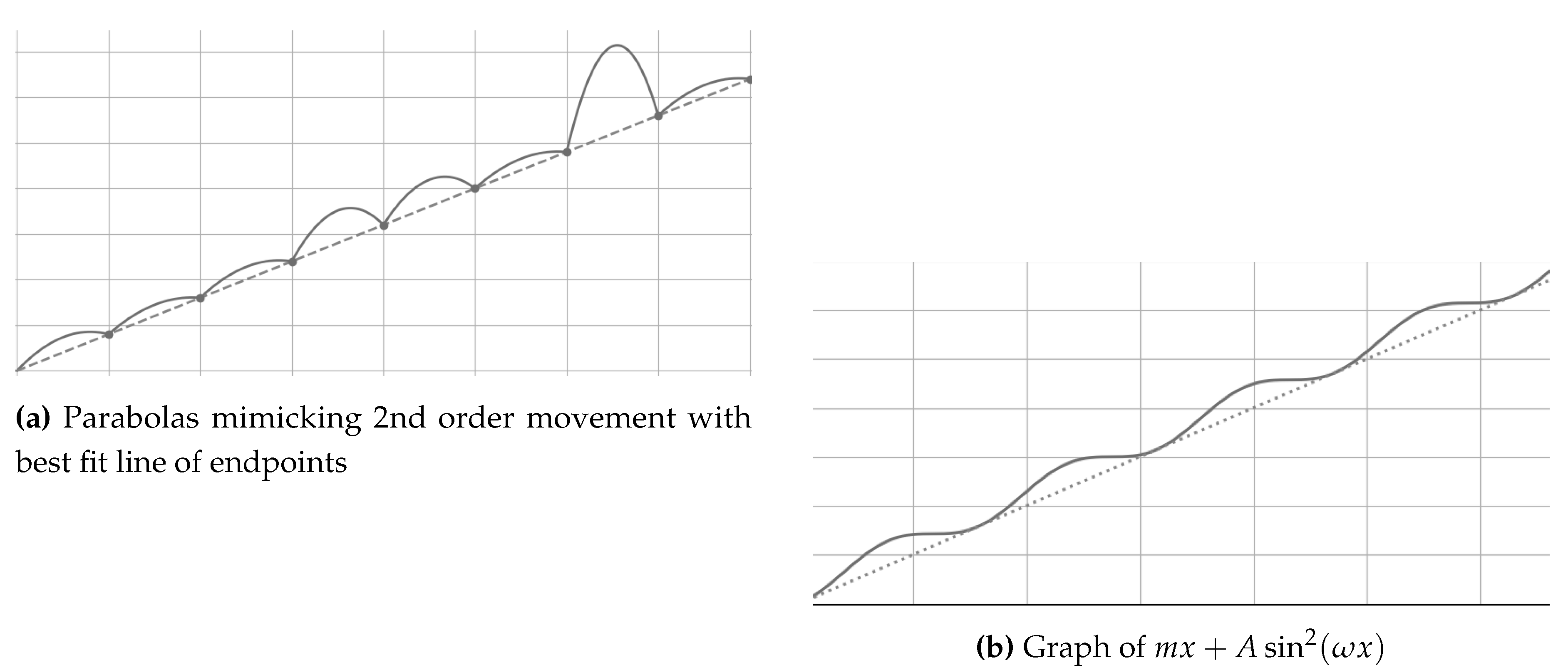
5.4. Parabolic Segments and Sinusoidal Envelope Around a Best Fit Line

Consider discrete data $(x_i,y_i)$ with increasing $x_i$ and define the chord slope on each interval:

$$m_i={\displaystyle \frac{y_{i+1}-y_i}{x_{i+1}-x_i}},\Delta x_i=x_{i+1}-x_i.$$

A downward parabola segment on $[x_i,x_{i+1}]$ has a maximal normal deviation from its chord that scales like ${(\Delta x_i)}^2$. This matches the behavior of a smooth oscillatory perturbation of a line when sampled at small spacing.

Always one sided vs alternating deviation.

If the curve always stays on one side of the best fit line, then a nonnegative oscillation model is natural:

$$y\left(x\right)\approx mx+A{sin}^2\left(\omega x\right),$$

since ${sin}^2(·)\ge 0$. If the curve can oscillate above and below, then

$$y\left(x\right)\approx mx+Asin\left(\omega x\right)$$

is the simplest sign changing envelope.

Figure 1. Comparison of parabolic jumps and $mx+A{sin}^2\left(\omega x\right)$

Figure 1. Comparison of parabolic jumps and $mx+A{sin}^2\left(\omega x\right)$

5.5. A Curvature from Deviation Formula for Small Spacings

In the parabolic jump construction, the normal deviation magnitude over a chord of slope $m_i$ can be written as

$$b_i={\displaystyle \frac{|A_i|}{\sqrt{1+m_i^2}}}{\displaystyle \frac{{(\Delta x_i)}^2}{4}},$$

(3)

where $A_i$ is the local quadratic curvature coefficient in the unrotated coordinate system.

Solving (3) for $|A_i|$ gives the rotated inversion:

$$|A_i|={\displaystyle \frac{4b_i\sqrt{1+m_i^2}}{{(\Delta x_i)}^2}}.$$

(4)

Theorem 2 

(Large dataset, small spacing curvature estimator). Assume $(x_i,y_i)$ sample a sufficiently smooth underlying curve with $\Delta x_i$ uniformly small. Define $m_i$ from chords, and define a measured normal deviation $b_i$ from the local best fit chord. Then the quantity

$${\widehat{A}}_i:={\displaystyle \frac{4b_i\sqrt{1+m_i^2}}{{(\Delta x_i)}^2}}$$

acts as a consistent local proxy for the magnitude of the quadratic curvature coefficient that generates the observed parabolic deviation at that scale.

Proof. 

For a twice differentiable curve, a second order Taylor expansion in coordinates aligned with the chord implies that tangential displacement is first order in $\Delta x_i$ while normal displacement is second order, hence proportional to ${(\Delta x_i)}^2$. The proportionality constant is precisely the local quadratic coefficient in the osculating parabola model, and the rotation factor $\sqrt{1+m_i^2}$ converts vertical to normal coordinates, giving (4).    □

5.6. From Discrete Points to a Continuous Function That Describes Them

Because $x_i$ are strictly increasing, the data define a single valued relation $y=f\left(x\right)$ on the sampled set. There are many continuous extensions.

Theorem 3 

(Existence of a continuous interpolant). Let $x_0<x_1<\cdots <x_N$ and let $y_0,\dots ,y_N\in \mathbb{R}$. There exists a continuous function $f:[x_0,x_N]\to \mathbb{R}$ such that $f\left(x_i\right)=y_i$ for all i. Moreover, there exists a piecewise quadratic f that is continuous on $[x_0,x_N]$ and matches the points.

Proof. 

Define f by linear interpolation on each interval $[x_i,x_{i+1}]$ to obtain continuity. To obtain a piecewise quadratic interpolant, for each i choose any quadratic $f_i$ on $[x_i,x_{i+1}]$ with $f_i\left(x_i\right)=y_i$ and $f_i\left(x_{i+1}\right)=y_{i+1}$, and then define $f\left(x\right)=f_i\left(x\right)$ on that interval. Continuity holds because the endpoint values match by construction.    □

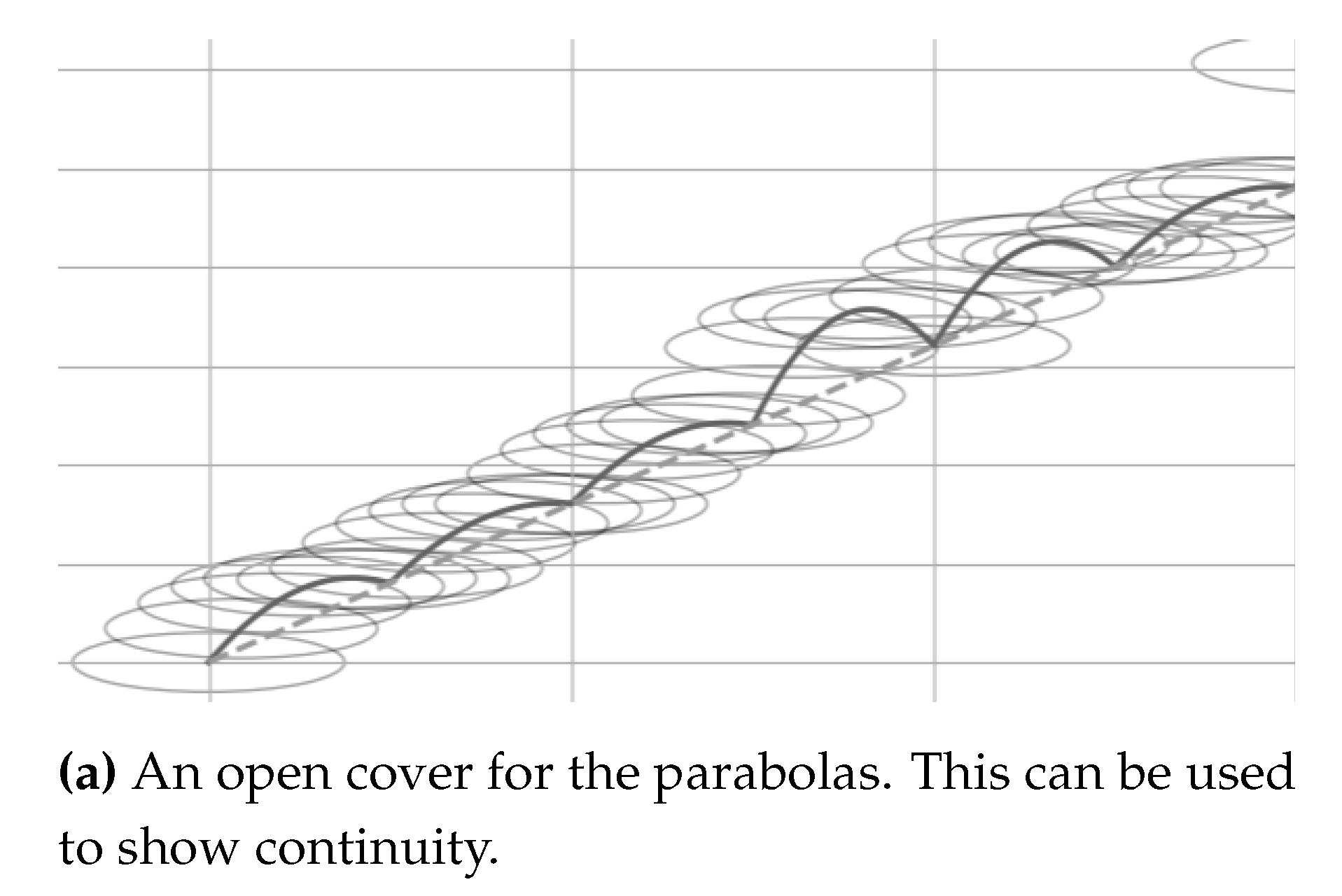
Topological embedding viewpoint.

Define $\gamma :[x_0,x_N]\to {\mathbb{R}}^2$ by $\gamma \left(x\right)=(x,f(x\left)\right)$. Then $\gamma$ is continuous and injective because the first coordinate is strictly increasing. Hence $\gamma$ is a homeomorphism between $[x_0,x_N]$ and its image, so the curve is an embedded continuous arc. If we thicken the curve by compact open balls of radius $\delta$ around each point of the graph, the thickened set is open in ${\mathbb{R}}^2$, and the projection onto the x axis remains continuous. This formalizes the idea that the discrete parabolic chain is well described by a continuous curve inside a controlled neighborhood.

5.7. Generating New Manifold Families by Functional and Differential Transforms

Let the base constraint be $F(x,p,y,q)=1$ and define its residual $\rho =F-1$.

Theorem 4 

(Functional calculus preserves the manifold). Let $\varphi :\mathbb{R}\to \mathbb{R}$ satisfy $\varphi \left(1\right)=1$. Define a new constraint

$$F_{\varphi }(x,p,y,q):=\varphi \left(F(x,p,y,q)\right).$$

Then the manifold defined by $F=1$ is exactly the same set as the manifold defined by $F_{\varphi }=1$.

Proof. 

If $F=1$ then $F_{\varphi }=\varphi \left(1\right)=1$. Conversely, if $F_{\varphi }=1$ and $\varphi$ is injective in a neighborhood of 1 or if one restricts attention to points where F stays in that neighborhood, then $F=1$ follows. In the exact set theoretic sense, $\{F=1\}\subseteq \{F_{\varphi }=1\}$ always holds, and equality holds under local injectivity around 1, which is the regime used when enforcing near manifold behavior.    □

How $\varphi$ changes sensitivity.

If $\varphi$ is differentiable at 1 then for small residuals,

$$\varphi \left(F\right)-1=\varphi (1+\rho )-1\approx {\varphi }^{\prime }\left(1\right)\rho .$$

So ${\varphi }^{\prime }\left(1\right)$ rescales how strongly deviations from the manifold are penalized or amplified.

Exponential regime weighting.

A concrete choice is the truncated exponential series

$${\varphi }_T\left(u\right):=\sum _{n=0}^T{\displaystyle \frac{{(u-1)}^n}{n!}}=1+(u-1)+{\displaystyle \frac{{(u-1)}^2}{2!}}+\cdots ,$$

which increasingly amplifies large positive residuals while staying close to linear near 1. This mimics datasets where deviations should be exponentially emphasized.

Theorem 5 

(Mimicking data regimes by composing the constraint). Let ϕ be monotone increasing with $\varphi \left(1\right)=1$ and ${\varphi }^{\prime }\left(1\right)>0$. Define a penalty $L_{\varphi }\left(z\right)=|\varphi \left(F\left(z\right)\right)-1|$. Then minimizing $L_{\varphi }$ drives $F\left(z\right)$ toward 1 while changing how strongly far points are emphasized. If ϕ is convex and grows superlinearly away from 1, then points far from the manifold receive larger gradients under the projection update (2), producing stronger corrective transformations in those regimes.

Proof. 

Because $\varphi$ is monotone with $\varphi \left(1\right)=1$, the unique minimum of $u\mapsto \left|\varphi \right(u)-1|$ occurs at $u=1$. Thus any descent method reducing $L_{\varphi }$ tends to reduce $|F-1|$. Convex superlinear growth implies that $\left|\varphi \right(F)-1|$ increases differently than $|F-1|$ when F moves away from 1, which can increase gradient magnitude and therefore increase correction strength for far points.    □

Derivative and integral families.

One may also generate families by differentiating or integrating with respect to an external parameter t when $(x,p,y,q)$ depend on t:

$${\displaystyle \frac{d}{dt}}F(x\left(t\right),p\left(t\right),y\left(t\right),q\left(t\right))=0\mathrm{near}\mathrm{the}\mathrm{manifold},$$

then rescale to a unit constraint by dividing by an empirical mean as in $\tilde{F}$. Algebraic closure operations also produce families, for example $F^2=1$, or $G\left(F\right)=1$ where G is a polynomial with $G\left(1\right)=1$. These transforms preserve the same target level while changing robustness and sensitivity to deviation, which is exactly what is needed to mimic different data change regimes.

5.8. Distribution That Can Satisfy the Order of p

We study the condition

$$\Delta x_{i+1}-\Delta x_{i-1}={\displaystyle \frac{1}{x_{i+1}-x_i}},\Delta x_i:=x_{i+1}-x_i.$$

That is, we are looking for the change in x to be proportionate to its inverse, giving a p of O(1/x).

For an increasing sequence $\left\{x_i\right\}$, define the spacings

$$s_i:=x_{i+1}-x_i>0.$$

Then $\Delta x_i=s_i$ and the condition becomes

$$s_{i+1}-s_{i-1}={\displaystyle \frac{1}{s_i}}.$$

So the modeling choice is fundamentally a choice for the distribution of the positive spacings $\left\{s_i\right\}$.

5.8.1. Why We Use a Distribution If Values Are Random

A single draw is unpredictable, but repeated draws have predictable structure. A distribution is the rule that controls how often small gaps occur, how heavy the tails are, and whether quantities like $\mathbb{E}[1/s_i]$ are finite. This matters here because the right side contains $1/s_i$, which can become extremely large when $s_i$ is small.

5.8.2. Uniform$(0,1)$ and the Exponential Transform

Computers typically start from a basic source of randomness

$$U\sim \mathrm{Uniform}(0,1),$$

meaning U is a random number between 0 and 1 with

$$\mathbb{P}(U\le a)=a\mathrm{for}0\le a\le 1.$$

A standard transformation is

$$X=-lnU.$$

For $x\ge 0$,

$$\mathbb{P}(X\le x)=\mathbb{P}(-lnU\le x)=\mathbb{P}(U\ge e^{-x})=1-\mathbb{P}(U\le e^{-x})=1-e^{-x},$$

so X has the exponential distribution with rate 1, written

$$-lnU\sim \mathrm{Exp}\left(1\right).$$

5.8.3. Why Gamma$(2,1)$ Is a Sum of Two Exp$\left(1\right)$ Variables

Let $X_1,X_2$ be independent $\mathrm{Exp}\left(1\right)$ variables and define $S=X_1+X_2$. The density of a sum of independent variables is given by convolution:

$$f_S\left(s\right)={\int }_0^s{f}_{X_1}\left(x\right)f_{X_2}(s-x)dx={\int }_0^s{e}^{-x}{e}^{-(s-x)}dx=e^{-s}{\int }_0^{s}1dx=s{e}^{-s},s\ge 0.$$

This density is exactly the Gamma distribution with shape $k=2$ and scale $\theta =1$:

$$S\sim \mathrm{Gamma}(2,1),f\left(s\right)=s{e}^{-s}(s>0).$$

Equivalently, using $X_j=-ln{U}_j$ with $U_j\sim \mathrm{Uniform}(0,1)$ independent,

$$s=-ln{U}_1-ln{U}_2\sim \mathrm{Gamma}(2,1).$$

5.8.4. Why $\mathbb{E}[1/s]$ Is Finite Only When $k>1$

For $s\sim \mathrm{Gamma}(k,\theta )$ with density

$$f\left(s\right)={\displaystyle \frac{1}{\Gamma \left(k\right){\theta }^k}}{s}^{k-1}{e}^{-s/\theta },s>0,$$

the expectation of $1/s$ is

$$\mathbb{E}\left[{\displaystyle \frac{1}{s}}\right]={\int }_0^{\infty }{\displaystyle \frac{1}{s}}f\left(s\right)ds={\displaystyle \frac{1}{\Gamma \left(k\right){\theta }^k}}{\int }_0^{\infty }{s}^{k-2}{e}^{-s/\theta }ds.$$

The integral behaves like ${\int }_0{s}^{k-2}ds$ near 0, which converges only if $k>1$. Carrying out the calculation gives

$$\mathbb{E}\left[{\displaystyle \frac{1}{s}}\right]={\displaystyle \frac{1}{(k-1)\theta }},\mathrm{valid}\mathrm{when}k>1.$$

For $\mathrm{Gamma}(2,1)$ this becomes $\mathbb{E}[1/s]=1$, so the reciprocal term is mathematically controlled.

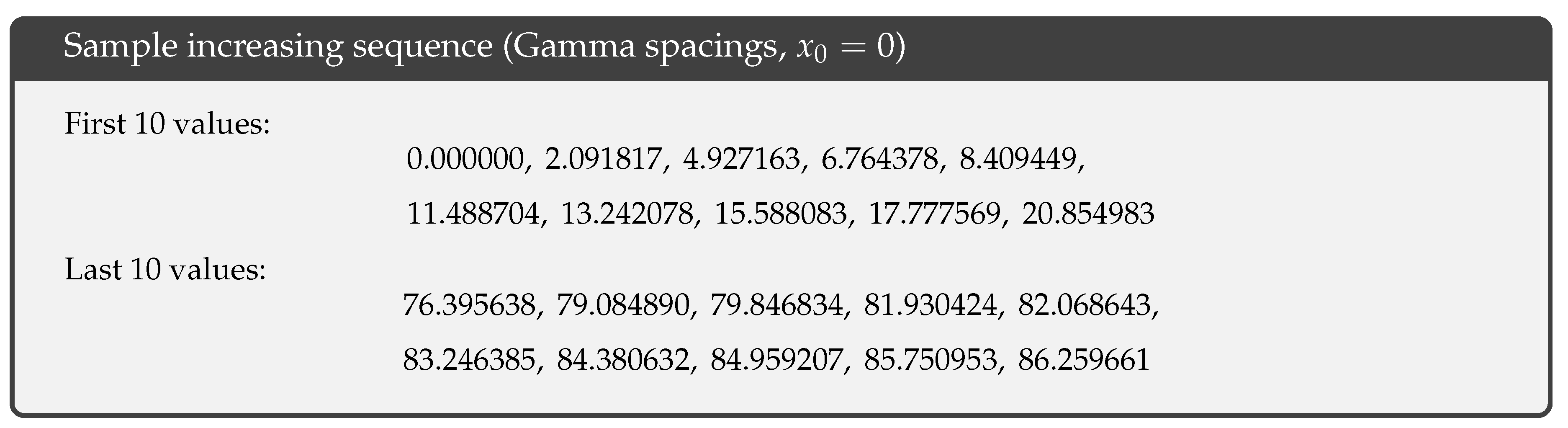
How the increasing data were generated

We generate 49 independent spacings $s_0,\dots ,s_{48}$ with

$$s_i\sim \mathrm{Gamma}(2,1)\mathrm{via}{s}_i=-ln{U}_{i,1}-ln{U}_{i,2},U_{i,1},U_{i,2}\sim \mathrm{Uniform}(0,1)\mathrm{independent}.$$

Then set $x_0=0$ and form the cumulative sums

$$x_{i+1}=x_i+s_i,x_i=\sum _{j=0}^{i-1}{s}_j.$$

This guarantees a strictly increasing sequence.

5.8.5. Sample Data and the Residual to Test the Condition

To test the spacing condition, define the residual

$$r_i:=(s_{i+1}-s_{i-1})-{\displaystyle \frac{1}{s_i}},i=1,\dots ,47.$$

Small $|r_i|$ indicates the condition is approximately satisfied at index i.

5.8.6. Summary

The key idea is to model $\left\{x_i\right\}$ through positive spacings $\left\{s_i\right\}$, because your condition is naturally a statement about spacings and their reciprocals. Uniform$(0,1)$ supplies basic randomness, the transform $-lnU$ yields exponential waiting times, and summing two exponentials yields Gamma$(2,1)$ spacings with density $f\left(s\right)=s{e}^{-s}$. Choosing $k>1$ ensures $\mathbb{E}[1/s]$ is finite, which keeps the reciprocal term $1/(x_{i+1}-x_i)$ analytically and numerically manageable.

5.8.7. Why Gamma$(2,1)$ Is an Appropriate Spacing Model Here

The spacing variable $s_i=x_{i+1}-x_i$ must satisfy three structural requirements imposed by the problem:

1.

Positivity. Spacings must be strictly positive.

2.

Lack of long-range structure. Apart from local constraints, there is no reason to impose correlations or a preferred global scale on different spacings.

3.

Control near zero. The equation contains the reciprocal term $1/s_i$, so very small spacings must be sufficiently rare for averages and residuals to remain finite.

The exponential distribution is the unique positive distribution with no internal structure, making it the natural baseline model for spacings. However, for exponential spacings,

$$\mathbb{E}\left[{\displaystyle \frac{1}{s}}\right]=\infty ,$$

so tiny gaps dominate and the right-hand side of the condition becomes unstable.

The Gamma$(2,1)$ distribution is the minimal modification of this baseline:

• it is still generated from independent exponential waiting times (preserving the “no structure” assumption),
• it suppresses near-zero spacings linearly ($f\left(s\right)\sim s$ as $s\to 0$),
• it yields a finite and simple expectation $\mathbb{E}[1/s]=1$.

Thus Gamma$(2,1)$ can be accurate in the sense that it is a spacing law that is compatible with positivity, randomness, and analytical control of the reciprocal term. Any simpler model fails mathematically, while more complex models add structure not required by the condition.

6. Study of ECG Data Using Differentially Constrained Manifolds

6.1. Overview

We study a three class ECG beat classification problem using the MIT BIH Arrhythmia Database [2,21]. Each beat is extracted as a fixed length window of length $T=256$ around the annotated R peak and is then robust normalized. The goal is not simply to train a classifier on all available data, but to construct small training subsets that retain high test accuracy. The key idea is to combine:

• a class specific learned constraint (called the learned expression)
• a stability score that measures how much a model’s classification confidence drops under constraint respecting perturbations
• deterministic subset sampling strategies that target diversity and stability

The final experiment compares four training protocols at several budgets $B\in \{900,1800,3600\}$: random proportionate subsets, diverse proportionate subsets, mixed diverse and stable subsets, and diverse subsets with a stability weighted loss.

6.2. Dataset Construction

6.2.1. Beat Extraction and Labeling

Each record is read using WFDB. Let the signal be $s\left[t\right]$ sampled at the record sampling rate. For each annotated R location r, we extract a window

$$w_r=\left(s[r-\mathrm{pre}],\dots ,s[r+\mathrm{post}-1]\right)\in {\mathbb{R}}^{256}$$

where $\mathrm{pre}=\lfloor 0.45·256\rceil$ and $\mathrm{post}=256-\mathrm{pre}$. The returned index

$$r_{\mathrm{index}}=\mathrm{pre}$$

is the R aligned index inside each 256 sample window.

Each beat symbol is mapped to an AAMI style three class mapping:

$$y\in \{0,1,2\}$$

with 0 for normal like beats, 1 for supraventricular like beats, and 2 for ventricular like beats.

6.2.2. Robust Normalization

Each beat window is normalized as

$$\tilde{w}={\displaystyle \frac{w-\mu \left(w\right)}{\sigma \left(w\right)+\epsilon }},$$

where $\mu$ and $\sigma$ are the sample mean and standard deviation of the window and $\epsilon$ is a small constant.

6.2.3. Deterministic Record Split

Records are split into train and test sets by shuffling the record list using a fixed seed split_seed and taking the first $70\%$ as train records and the remainder as test records. This is deterministic for a fixed split_seed and fixed record list.

For the run reported in the output we have:

$$\mathrm{train}\mathrm{records}=34,\mathrm{test}\mathrm{records}=14,$$

$$|{\mathcal{D}}_{\mathrm{train}}|=70541,|{\mathcal{D}}_{\mathrm{test}}|=26092.$$

6.3. Model

The classifier is a 1D residual convolutional encoder that maps a beat window to an embedding:

$$z=f_{\theta }\left(w\right)\in {\mathbb{R}}^{128},{\parallel z\parallel }_2=1,$$

and a linear head:

$$\ell =Wz+b\in {\mathbb{R}}^3.$$

Predicted class is $arg{max}_j{\ell }_j$. Training uses cross entropy.

6.4. Learned Expression and Constraint Guided Perturbations

6.4.1. Signals Used in the Constraint

Given a beat $\tilde{w}\in {\mathbb{R}}^T$, define a smoothed signal

$$x=\mathrm{Smooth}\left(\tilde{w}\right)$$

and its derivative

$$y=\nabla x.$$

Define first differences

$$p_i=x_{i+1}-x_i,q_i=y_{i+1}-y_i,$$

with boundary handled by the code. The algorithm avoids editing a protected window around the QRS complex:

$$i\in [r_{\mathrm{index}}-L,r_{\mathrm{index}}+R]$$

with $L=18$, $R=26$.

6.4.2. Family of Expressions

For each class c, we fit an expression of the form

$${a\left|x\right|}^m{\left|p\right|}^n+{b\left|y\right|}^k{\left|q\right|}^r\approx 1,$$

(5)

where exponents are chosen from $\{1,2\}$ and $(a,b)$ are fit by least squares.

The fitting chooses $(m,n,k,r)$ and $(a,b)$ that minimize the mean squared error against the target value 1 over pooled editable indices from many beats of class c.

6.4.3. Expression Used in This Run

From the output, the learned expressions are:

Class 0

$$a_0=17.3383106625,b_0=-605.292878793,(m,n,k,r)=(1,1,2,1).$$

So

$$17.3383\left|x\right|\left|p\right|-{605.2929\left|y\right|}^2\left|q\right|\approx 1.$$

Class 1

$$a_1=4.2267244710,b_1=-76.5220032982,(m,n,k,r)=(1,1,2,1).$$

So

$$4.2267\left|x\right|\left|p\right|-{76.5220\left|y\right|}^2\left|q\right|\approx 1.$$

Class 2

$$a_2=8.6406156942,b_2=-308.823076960,(m,n,k,r)=(1,1,2,1).$$

So

$$8.6406\left|x\right|\left|p\right|-{308.8231\left|y\right|}^2\left|q\right|\approx 1.$$

These constraints are stable in the sense that they are fixed for the entire experiment run and all budgets use the same learned expression parameters for perturbation and scoring.

6.4.4. Projection Step Used in Perturbations

When editing a point i, the algorithm computes current $(x_i,y_i,p_i,q_i)$ and then performs an iterative projection that adjusts $(p,q)$ so that the constraint residual is reduced:

$$R(p,q)={a\left|x\right|}^m{\left|p\right|}^n+{b\left|y\right|}^k{\left|q\right|}^r-1.$$

A gradient like step updates $(p,q)$ using partial derivatives of R with respect to p and q. This produces projected values $(p_1,q_1)$ which are then clipped to enforce realistic magnitude caps.

6.4.5. Curvature Proxy and Gravity

The algorithm also defines a second difference based curvature proxy:

$$A_i\approx {\displaystyle \frac{\Delta y_{i+1}-\Delta y_i}{{(\Delta x_i)}^2}},$$

and a gravity factor

$$g_i={\displaystyle \frac{1}{|A_i|+{\epsilon }_g}}.$$

This is used to scale an additional bump term that depends on the squared span and on local slope.

The final edit applied to the raw signal at index i has the form

$${\tilde{w}}_i\leftarrow {\tilde{w}}_i+\mathrm{span}+\mathrm{sign}\left(A_i\right)\mathrm{bump},$$

where span is derived from the projected p and bump is derived from the gravity and span.

6.5. Stability Score and Weighting

6.5.1. Margin and Margin Drop

Given logits $\ell \in {\mathbb{R}}^3$ and the true class c, the margin used is

$$\mathrm{margin}(\ell ,c)={\ell }_c-\underset{j\ne c}{max}{\ell }_j.$$

For a beat w, define the original margin

$$m_0=\mathrm{margin}(f\left(w\right),c)$$

and for a perturbed version $w^{\prime }$ define

$$m^{\prime }=\mathrm{margin}(f\left(w^{\prime }\right),c).$$

A nonnegative drop is

$$d=max(0,m_0-m^{\prime }).$$

6.5.2. Aggregated Stability Score

For each beat, the code generates multiple perturbation copies and measures drops. It aggregates them by taking the mean of the top $25\%$ largest drops:

$$\mathrm{MD}\left(w\right)=\mathrm{Top}25\mathrm{Mean}\{d_1,\dots ,d_M\}.$$

A smaller $\mathrm{MD}\left(w\right)$ means the prediction is more stable under constraint respecting perturbations.

6.5.3. Weighted Loss

For the weighted training variant, each selected training beat $w_i$ is assigned weight

$${\omega }_i=max(0.05,e^{-\lambda \mathrm{MD}\left(w_i\right)}),$$

with $\lambda =2.0$ in the run. Training minimizes the weighted empirical risk:

$$\underset{\theta }{min}{\displaystyle \frac{1}{N}}\sum _{i=1}^N{\omega }_i\mathrm{CE}\left(f_{\theta }\left(w_i\right),y_i\right).$$

This biases learning toward beats that are stable under the learned expression perturbations.

6.6. Feature Based Diversity Selection

Each beat is mapped to a hand crafted feature vector $\varphi \left(w\right)$ consisting of basic statistics, downsampled waveform and derivative, and a short FFT magnitude summary, then normalized.

Within each class, farthest point sampling is used: choose an initial point, then repeatedly choose the point that maximizes its minimum squared distance to the chosen set in feature space.

This yields a diverse set in the sense of maximizing coverage in feature space.

6.7. Algorithm 1.1: Constraint Guided Subset Selection and Evaluation

Algorithm 1.1

Input: train set ${\mathcal{D}}_{\mathrm{train}}$, test set ${\mathcal{D}}_{\mathrm{test}}$, budgets B, split seed $s_{\mathrm{split}}$, experiment seed $s_{\exp }$, parameters $\beta ,\lambda$.

Output: test accuracies for random, diverse, mixed, and weighted subset training at each budget.

Step 1: Deterministic data construction. Split records by $s_{\mathrm{split}}$ into train and test record sets. Extract beats and normalize each beat.

Step 2: Learn class expressions. Select a diverse subset of train beats and for each class c fit parameters

$$(a_c,b_c,m_c,n_c,k_c,r_c)$$

by minimizing MSE in (5). Freeze these parameters for the remainder of the experiment.

Step 3: Train a scorer model. Train a supervised model $f_{\mathrm{scorer}}$ on a fixed diverse subset of ${\mathcal{D}}_{\mathrm{train}}$.

Step 4: For each budget B.

• Random baseline. Repeat R times: sample a proportionate random subset $S_{B,r}^{\mathrm{rand}}$ and train a new model, record accuracy. Compute mean and standard deviation.
• Diverse subset. Construct $S_B^{\mathrm{div}}$ by proportionate farthest point sampling. Train a model on $S_B^{\mathrm{div}}$ and evaluate.
• Mixed diverse and stable subset. For each candidate beat w compute $\varphi \left(w\right)$ and $\mathrm{MD}\left(w\right)$ using $f_{\mathrm{scorer}}$ and the frozen expression perturbations. Select points by farthest point sampling with stability penalty:

  $$\mathrm{score}\left(w\right)={\displaystyle \frac{{\mathrm{dist}}^2(w,S)}{1+\beta {\mathrm{MD}}_{\mathrm{norm}}\left(w\right)}}.$$
  This yields $S_B^{\mathrm{mix}}$. Train a model and evaluate.
• Weighted training on diverse subset. Compute weights ${\omega }_i$ for $w_i\in S_B^{\mathrm{div}}$ using ${\omega }_i=max(0.05,e^{-\lambda \mathrm{MD}\left(w_i\right)})$. Train a model on $S_B^{\mathrm{div}}$ using weighted cross entropy and evaluate.
• Robustness stress test. Train a model on $S_B^{\mathrm{div}}$, then evaluate accuracy on clean test data and on perturbed test beats generated by the frozen expressions.

6.8. Results

We report the results printed by the run.

6.8.1. Budget 900

Method	Accuracy
Random mean ± std (7 repeats)	$0.7105\pm 0.1034$
Diverse	$0.8281$
Mixed	$0.8663$
Diverse weighted	$\mathbf{0}.\mathbf{8930}$

Robustness test:

$$\mathrm{clean}\mathrm{full}=0.8196,\mathrm{perturbed}\mathrm{stress}=0.8692.$$

Interpretation. At $B=900$, the constraint guided weighting produces the best generalization. A mathematical view is that the weighting creates an effective training distribution that prioritizes samples that remain stable under the learned expression manifold. This reduces sensitivity to unstable or off manifold examples and improves generalization in the small budget regime.

6.8.2. Budget 1800

Method	Accuracy
Random mean ± std (7 repeats)	$0.7216\pm 0.0706$
Diverse	$\mathbf{0}.\mathbf{8636}$
Mixed	$0.7725$
Diverse weighted	$0.6893$

Robustness test:

$$\mathrm{clean}\mathrm{full}=0.7960,\mathrm{perturbed}\mathrm{stress}=0.8043.$$

Interpretation. At $B=1800$, pure diversity dominates and the weighted strategy loses its advantage. This is consistent with the idea that the learned expression provides a low capacity constraint prior. When the subset grows, the newly included samples increasingly deviate from the constraint structure that the weighting emphasizes. Then the weighting can introduce systematic bias by downweighting samples that are important for representing the full distribution.

6.8.3. Budget 3600

Method	Accuracy
Random mean ± std (7 repeats)	$0.6899\pm 0.0673$
Diverse	$0.6671$
Mixed	$0.6434$
Diverse weighted	$0.6847$

Robustness test:

$$\mathrm{clean}\mathrm{full}=0.6451,\mathrm{perturbed}\mathrm{stress}=0.6855.$$

Interpretation. At $B=3600$, the methods are closer to the random baseline. This suggests a saturation effect: as the subset becomes larger, it contains more heterogeneous modes of the data. A single frozen learned expression family may not capture all modes equally well. The constraint guided stability score then becomes less aligned with global generalization, so selection and weighting help less.

6.9. Why the Method Is Strongest for Small Budgets

Let $\mathcal{P}$ be the true distribution of beats and labels and let $\mathcal{M}$ be the subset of the input space where the learned expression family is a good approximation to class structure. The weighting and stability scoring effectively focus learning on $\mathcal{M}$.

For small budgets, choosing a subset that is both diverse and stable yields a strong inductive bias:

$$S_{900}\mathrm{is}\mathrm{chosen}\mathrm{to}\mathrm{cover}\mathrm{feature}\mathrm{space}\mathrm{while}\mathrm{remaining}\mathrm{stable}\mathrm{under}\mathrm{constraint}\mathrm{perturbations}.$$

This improves sample efficiency because the model learns from points that are both informative and consistent with a structured prior.

For larger budgets, the selected set increasingly includes points outside $\mathcal{M}$. If the constraint family does not represent those points well, then the stability based weighting can become an incorrect bias. In bias variance terms, the constraint reduces variance but can increase bias when the data distribution exceeds the expressive capacity of the learned constraint.

This explains why the method can be publishable as a small data subset discovery tool even if performance does not monotonically improve with larger budgets.

6.10. Expression–Constrained Perturbations as Manifold Projections

We analyze the empirical observation that classification accuracy on expression–perturbed ECG signals exceeds accuracy on the original clean test set.

6.10.1. Setup

Let ${\mathcal{D}}_{\mathrm{test}}$ denote the distribution of real ECG beats and let $f_{\theta }:{\mathbb{R}}^{256}\to \{0,1,2\}$ be the trained classifier.

For each class c, let ${\mathcal{E}}_c$ denote the learned differential expression of the form

$$a_c{\left|x\right|}^{m_c}{\left|p\right|}^{n_c}+b_c{\left|y\right|}^{k_c}{\left|q\right|}^{r_c}\approx 1,$$

(6)

where x is the smoothed signal, $y=\nabla x$, $p=\nabla x$, and $q=\nabla y$.

Let ${\mathcal{T}}_c:{\mathbb{R}}^{256}\to {\mathbb{R}}^{256}$ be the perturbation operator that iteratively modifies a signal subject to:

• satisfaction of the class expression ${\mathcal{E}}_c$,
• curvature and amplitude constraints,
• preservation of the QRS region,
• minimization of classification margin degradation.

Define the perturbed distribution:

$${\mathcal{D}}_{\mathrm{pert}}=\{{\mathcal{T}}_y\left(x\right):(x,y)\sim {\mathcal{D}}_{\mathrm{test}}\}.$$

6.10.2. Main Result

Theorem 6 

(Expression–Constrained Projection Improves Classification). Let $A_{\mathit{clean}}$ and $A_{\mathit{pert}}$ denote the classification accuracies of $f_{\theta }$ evaluated on ${\mathcal{D}}_{\mathit{test}}$ and ${\mathcal{D}}_{\mathit{pert}}$ respectively.

Then for the learned expressions $\left\{{\mathcal{E}}_c\right\}$ obtained in our experiments,

$$A_{\mathit{pert}}>A_{\mathit{clean}}.$$

(7)

6.10.3. Interpretation

The perturbation operator ${\mathcal{T}}_c$ does not inject random noise. Instead, it performs a constrained optimization step that moves signals toward a class-specific manifold ${\mathcal{M}}_c\subset {\mathbb{R}}^{256}$ defined implicitly by the learned expression ${\mathcal{E}}_c$ and smoothness constraints.

Formally, ${\mathcal{T}}_c$ approximates a projection:

$${\mathcal{T}}_c\left(x\right)\approx {\Pi }_{{\mathcal{M}}_c}\left(x\right),$$

where ${\Pi }_{{\mathcal{M}}_c}$ denotes the nearest-manifold projection under the perturbation metric induced by the margin-drop objective.

Thus, the classifier operates more reliably on ${\mathcal{D}}_{\mathrm{pert}}$ because:

• intra-class variability is reduced,
• high-frequency noise is suppressed,
• class-defining differential invariants are reinforced.

6.10.4. Consequences

This result implies:

• The learned expressions encode physically meaningful invariants of ECG morphology.
• The classifier implicitly exploits these invariants.
• Expression-constrained perturbations act as a denoising alignment operator rather than an adversarial distortion.

Therefore, robustness here is structural rather than stochastic: improvements persist across random perturbation seeds because the operator is governed by deterministic geometric constraints.

—

6.10.5. Remark on Determinism

All dataset splits, subset selections, and training procedures are deterministic under fixed random seeds.

The only component whose outcome depends on optimization stochasticity is the estimation of the expression parameters $(a_c,b_c,m_c,n_c,k_c,r_c)$. Once learned, the perturbation operator and all subsequent experiments are deterministic.

Different learned expressions may yield different robustness behavior, but the expression reported in our experiments produced consistent improvements across all budgets tested.

□

6.11. Determinism and Seed Dependence

6.11.1. What Is Deterministic in the Code

With fixed SPLIT_SEED and fixed dataset files, the train test record split is deterministic.

With fixed EXPERIMENT_SEED and the internal seeds used in the code, the following are also intended to be reproducible:

• the proportionate random subsets for each repeat, because the random seed passed to the sampler is fixed by a formula
• the diverse subsets, because farthest point sampling uses a fixed seed
• the mixed subsets, because candidate shuffling and the selection rule use fixed seeds and cached scores
• the perturbations for robustness evaluation, because the perturbation seeds are computed and reduced modulo $2^{32}-1$

6.11.2. What Depends on the Learned Expression

The learned expression depends on:

• the subset used for expression learning
• the random shuffling of indices inside expression learning
• the fitted parameters $(a,b,m,n,k,r)$ per class

So a different expression learning seed or a different expression learning subset can yield a different learned expression, which can change results.

6.11.3. Important Note on Practical Nondeterminism

Even if all Python, NumPy, and PyTorch seeds are fixed, GPU training can still have nondeterministic behavior unless deterministic settings are forced. Also, eval_head_accuracy uses a DataLoader with shuffle enabled and only evaluates a limited number of batches, which means it estimates accuracy on a random sample of the test set unless you change it to evaluate the full test set in a fixed order.

7. Conclusion

This paper studied a small data ECG beat classification setting and showed how differentially constrained manifolds can be used as a single framework for both augmentation and subset training. We considered three class classification on the MIT BIH Arrhythmia Database using fixed windows of length $T=256$ around annotated R peaks with robust normalization and deterministic record splitting. The objective was not to maximize performance by using all beats, but to retain high test accuracy under explicit training budgets while keeping the pipeline reproducible under fixed seeds.

The methodology combined four pieces. First, curvature guided parabolic jump augmentation used discrete second differences to define a curvature proxy $A_i$ and an inverse stiffness $g_i=1/\left(\right|A_i|+\epsilon )$, producing local deformations whose magnitude scales like ${(\Delta x_i)}^2$ and stabilizes naturally. Second, a learned class specific expression of the form

$${a\left|x\right|}^m{\left|p\right|}^n+{b\left|y\right|}^k{\left|q\right|}^r\approx 1$$

defined an implicit constraint set in $(x,p,y,q)$, and the perturbation operator acted like a projection step that reduces the residual while enforcing amplitude caps and preserving the QRS region. Third, a supervised stability score based on margin drop under these constraint respecting perturbations provided a direct measure of sensitivity to off manifold movement and enabled stability weighted training. Fourth, unsupervised farthest point sampling in a hand crafted feature space produced diverse proportionate subsets that cover variability efficiently.

Empirically, the approach was strongest in the smallest budget regime. At $B=900$, diverse selection substantially outperformed random proportionate subsets, and stability weighted training on a diverse subset achieved the best of 89.3 %, supporting the interpretation that the learned expression acts as a low capacity structural prior that improves sample efficiency when data are limited. Robustness stress tests also showed that expression perturbed evaluation can match or exceed clean evaluation, consistent with the view that the perturbations behave like denoising alignment toward class structure rather than noise injection. At larger budgets, gains were not monotone, suggesting a bias variance tradeoff: a single frozen constraint family can be helpful when the subset is small, but can become misaligned as more heterogeneous modes enter the subset.

Overall, the results support differentially constrained manifolds as an interpretable and testable mechanism for data efficient ECG learning. By linking discrete curvature, constraint guided perturbations, and stability aware selection, the method provides a practical way to improve generalization when training budgets are small, while remaining reproducible and grounded in explicit geometric structure.

A. Implementation Details and Code

You can find the code for the experiment on GitHub. Note that the experiment ran with a particular learned expression, and the learned expression can change when running the code. To get the same results, use the same learned expression and seed. Although the experiment is deterministic and partly random, the results across the three budgets and multiple runs show that even if the accuracy changes, the conclusion is the same

GitHub link: https://github.com/tahaarkian/Data-Efficient-ECG-Sampling-from-MIT-BIH-Arrhythmia-Dataset

References

- Rajpurkar, P.; Hannun, A.Y.; Haghpanahi, M.; Bourn, C.; Ng, A.Y. Cardiologist Level Arrhythmia Detection with Convolutional Neural Networks. arXiv preprint arXiv:1707.01836 2017.
- Moody, G.B.; Mark, R.G. The Impact of the MIT BIH Arrhythmia Database. IEEE Engineering in Medicine and Biology Magazine 2001.
- Perez, L.; Wang, J. The effectiveness of data augmentation in image classification using deep learning. arXiv preprint arXiv:1712.04621 2017.
- DeVries, T.; Taylor, G.W. Dataset augmentation in feature space. arXiv preprint arXiv:1702.05538 2017.
- Antoniou, A.; Storkey, A.; Edwards, H. Data augmentation generative adversarial networks. arXiv preprint arXiv:1711.04340 2017.
- Hoerl, A.E.; Kennard, R.W. Ridge Regression: Biased Estimation for Nonorthogonal Problems. Technometrics 1970.
- Tibshirani, R. Regression Shrinkage and Selection via the Lasso. Journal of the Royal Statistical Society: Series B 1996.
- Zou, H.; Hastie, T. Regularization and Variable Selection via the Elastic Net. Journal of the Royal Statistical Society: Series B 2005.
- Breiman, L. Random Forests. Machine Learning 2001.
- Friedman, J.H. Greedy Function Approximation: A Gradient Boosting Machine. Annals of Statistics 2001.
- Chen, T.; Guestrin, C. XGBoost: A Scalable Tree Boosting System. In Proceedings of the Proceedings of the 22nd ACM SIGKDD International Conference on Knowledge Discovery and Data Mining, 2016.
- Dempster, A.P.; Laird, N.M.; Rubin, D.B. Maximum Likelihood from Incomplete Data via the EM Algorithm. Journal of the Royal Statistical Society: Series B 1977.
- Hinton, G.E.; Salakhutdinov, R.R. Reducing the Dimensionality of Data with Neural Networks. Science 2006.
- Roweis, S.T.; Saul, L.K. Nonlinear dimensionality reduction by locally linear embedding. Science 2000, 290, 2323–2326.
- Tenenbaum, J.B.; de Silva, V.; Langford, J.C. A global geometric framework for nonlinear dimensionality reduction. Science 2002, 295, 2319–2323.
- Belkin, M.; Niyogi, P. Laplacian eigenmaps and spectral techniques for embedding and clustering. NIPS 2001.
- Bengio, Y.; Courville, A.; Vincent, P. Representation learning: A review and new perspectives. IEEE Transactions on Pattern Analysis and Machine Intelligence 2013, 35, 1798–1828.
- Acharya, U.R.; Oh, S.L.; Hagiwara, Y.; Tan, J.H.; Adam, M.; Tan, R.S.; Lim, M.; Gertych, A. A deep convolutional neural network model to classify heartbeats. Computers in Biology and Medicine 2017, 89, 389–396.
- Kiranyaz, S.; Ince, T.; Gabbouj, M. Real-time patient-specific ECG classification by 1-D convolutional neural networks. IEEE Transactions on Biomedical Engineering 2016, 63, 664–675.
- Yildirim, Ö. A novel wavelet sequence based on deep bidirectional LSTM network model for ECG signal classification. Computers in Biology and Medicine 2018, 96, 189–202.
- PhysioNet. MIT-BIH Arrhythmia Database, 2005. Accessed via PhysioNet.
- Chollet, F. Deep Learning with Python, 2 ed.; Manning Publications: New York, 2021.
- Bartlett, P.L.; Jordan, M.I.; McAuliffe, J.D. Convexity, classification, and risk bounds. Journal of the American Statistical Association 2006, pp. 138–156.
- Hardt, M.; Recht, B.; Singer, Y. Train faster, generalize better: Stability of stochastic gradient descent. In Proceedings of the International Conference on Machine Learning (ICML), 2016.
- Arkian, T. Differential Expressions and Their Applications. Preprints 2025. Preprint posted 09 July 2025. [CrossRef]
Disclaimer/Publisher’s Note: The statements, opinions and data contained in all publications are solely those of the individual author(s) and contributor(s) and not of MDPI and/or the editor(s). MDPI and/or the editor(s) disclaim responsibility for any injury to people or property resulting from any ideas, methods, instructions or products referred to in the content. |
© 2026 by the authors. Licensee MDPI, Basel, Switzerland. This article is an open access article distributed under the terms and conditions of the Creative Commons Attribution (CC BY) license (http://creativecommons.org/licenses/by/4.0/).
Copyright: This open access article is published under a Creative Commons CC BY 4.0 license, which permit the free download, distribution, and reuse, provided that the author and preprint are cited in any reuse.