
Submitted:
05 February 2026
Posted:
06 February 2026
You are already at the latest version
Abstract
Accurate Land Use and Land Cover (LULC) mapping in high-latitude mountain regions faces critical challenges from persistent cloud cover and complex topography, factors which limit the utility of passive optical sensors. To address the lack of operational guidelines for these data-scarce environments, this study establishes a transferable geospatial workflow based on a systematic ablation design to quantify the marginal and synergistic contributions of optical data (Sentinel-2), Synthetic Aperture Radar (Sentinel-1 SAR), topography, and intra-seasonal phenological metrics within the Aysén River basin, Chilean Patagonia. Using a Random Forest classifier, we implemented a progressive integration framework to compare a seasonal optical baseline model (A) against configurations incorporating intra-seasonal percentiles (A+P), topography (A+T), SAR (A+R), and their full integration (A+P+T+R). While the baseline model achieved an Overall Accuracy (OA) of 89.2% and a Macro-F1 of 80.5%, the fully integrated model reached an OA of 92.5% and a Macro-F1 of 86.0%. Notably, the inclusion of structural information from SAR and topography was decisive in improving the discrimination of complex vegetation classes, contributing to a net increase of +5.5 percentage points in the Macro-F1 score. Furthermore, the analysis revealed that annual SAR composites offer superior spatial consistency compared to seasonal aggregations, which introduce geometric artifacts despite high statistical metrics. These results demonstrate that the proposed structural–spectral integration framework resolves persistent ambiguities in transitional zones, providing a robust, replicable solution for ecosystem monitoring in complex high-latitude environments.
Keywords:
cloud computing
; Google Earth Engine
; sentinel-1/sentinel-2 fusion
; random forest
; intra-seasonal phenology
; persistent cloud cover
; Andean ecosystems
; Patagonia
1. Introduction
Accurate monitoring of Land Use and Land Cover (LULC) dynamics is essential for achieving the Sustainable Development Goals (SDGs) and supporting climate mitigation strategies advanced by the Intergovernmental Panel on Climate Change (IPCC) [1]. Over the past decade, the open-data policies of Earth observation missions such as Landsat and Copernicus Sentinel, together with the democratization of high-performance cloud computing through platforms like Google Earth Engine (GEE), have transformed global observation capabilities and enabled large-scale, multi-temporal analyses across spatial scales [2].
Despite these advances, the production of systematic LULC maps in mountainous ecosystems remains severely constrained, even when machine-learning classifiers are employed [3,4]. Persistent cloud cover creates substantial data gaps in optical time series, while complex topography introduces radiometric distortions that degrade model performance [5].
This observational deficit has produced a critical geographic and thematic bias within the national literature. A recent systematic review [6] shows that LULC research in Chile is disproportionately concentrated in the central region, whereas areas such as Aysén and Magallanes account for less than 2% of published studies. This gap is particularly concerning given that the Chilean Patagonia represents a globally significant natural laboratory, characterized by a pronounced west–east ecological gradient encompassing temperate forests, shrublands, steppes, and wetlands [7,8]. Moreover, the limited monitoring efforts conducted to date have primarily focused on forest dynamics, leaving substantial gaps in the characterization of transitional land-cover classes. These classes are frequently misclassified in official static inventories and global products [6,9,10,11].
To overcome these limitations, it is necessary to move beyond traditional optical-only approaches. The combined use of robust statistics derived from the temporal distribution (e.g., medians and percentiles such as and ) has become an effective strategy for mitigating atmospheric noise and capturing phenological variability in optical time series, even under limited observation availability [12]. Nevertheless, exclusive reliance on optical data remains a vulnerability at austral latitudes [13]. Consequently, the integration of Synthetic Aperture Radar (SAR), particularly Sentinel-1, emerges as a critical complementary solution by providing information on physical structure and surface roughness that is independent of atmospheric conditions [14]. In environments characterized by abrupt relief, however, effective SAR use requires the explicit incorporation of topographic variables, not only to contextualize the radar signal as a function of terrain geometry but also to represent ecologically relevant altitudinal gradients [15].
Within this context, the present study implements a systematic ablation experimental design in the Aysén River Basin to quantify the relative and complementary contributions of the optical, topographic, and radar domains to LULC classification. Three working hypotheses are formulated, linking sensor physical properties to landscape structure:
1.Phenological Hypothesis (H1): Distribution-based percentile metrics are expected to capture the amplitude of phenological signals more effectively than measures of central tendency, enabling the discrimination of spectrally similar land covers with contrasting intra-annual dynamics (e.g., deciduous versus evergreen vegetation).
2. Structural Hypothesis (H2): The inclusion of SAR backscatter from Sentinel-1 is hypothesized to provide information orthogonal to optical reflectance, facilitating land-cover discrimination based on surface roughness and volumetric structure, particularly for classes with contrasting architectures (e.g., urban areas versus bare soil).
3.Topo-Ecological Hypothesis (H3): Topographic variables are anticipated to act as environmental proxies of the altitudinal gradient, constraining the spatial probability of class occurrence and reducing thematic confusion in Andean transition zones (e.g., vegetation, snow, and wetland distributions).
2. Materials and Methods
2.1. Study Area
The Aysén River basin is located in the Aysén del General Carlos Ibáñez del Campo Region of southern Chilean Patagonia, situated approximately between 45°00′–46°16′ S and 71°20′–73°00′ W (Figure 1). According to the official delimitation by the General Water Directorate’s (DGA) National Inventory of Hydrographic Basins, the basin covers a total area of 1,142,537 ha.
The territory is characterized by rugged topography, extending from sea level at the Aysén Fjord to the Andean summits. The basin’s relief rises progressively from the eastern valleys to the Andes Mountains in the west, where the highest altitudes and steepest slopes occur. Elevations in this sector reach 2,227 m a.s.l., with a mean slope of 32% [16].
Climatically, the basin exhibits a marked west-to-east gradient. In the western sector, annual precipitation exceeds 3,000–4,000 mm, accompanied by persistent cloud cover, which fosters the development of temperate evergreen forests and Lenga (Nothofagus pumilio) stands [16,17]. Eastward, precipitation drops to 621 mm annually in Balmaceda, where Patagonian steppes predominate under a cold, dry climate [7]. This environmental contrast drives an ecologically significant biogeographical transition from coastal rainforests to inland semi-arid environments.
Furthermore, the current landscape configuration of the Aysén River basin is the direct result of massive and singular anthropogenic disturbance. Historically, during the agro-livestock colonization period (late 19th to mid-20th century), the basin underwent massive and systematic burning of native forest to clear land for pasture [18]. It is estimated that nearly 60% of the original forest was destroyed, causing severe fragmentation and loss of landscape connectivity [7,16]. The western sector was the most severely affected; here, the loss of vegetation cover promotes soil erosion and prompted reforestation programs using exotic species, primarily Pinus spp. These plantations altered the landscape structure and evolved into a relevant productive component for the region [16]. This legacy of degradation has generated vast transition zones or anthropogenic ecotones, composed of dense secondary shrublands (Nothofagus antarctica), degraded grasslands, and matrices of standing deadwood.
As a result of the interaction between these natural and anthropogenic factors, the Aysén River basin currently exhibits a highly heterogeneous environmental mosaic. Temperate rainforests, peatlands, shrublands, agricultural grasslands, rocky areas, snow, and glaciers coexist within the territory alongside productive zones and dispersed settlements. This topographical, climatic, and historical diversity reflects the environmental and socio-ecological transformations of the 20th century, rendering the basin a representative landscape of Chilean Patagonia where processes of conservation, productive use, and ecological regeneration converge [7,18].
2.2. Data Acquisition
The satellite and topographic data employed in this study consist of public products from the Sentinel-2, Sentinel-1, and SRTM missions, accessed and processed via the Google Earth Engine platform [19].
2.2.1. Sentinel-2 (Optical)
We employed images from the Multispectral Instrument (MSI) onboard the Sentinel-2A and Sentinel-2B satellites, part of the European Space Agency’s (ESA) Copernicus program. The products used correspond to Level-2A (Surface Reflectance), obtained via Sen2Cor atmospheric correction from Level-1C data [20]. This processing level provides surface reflectance suitable for land use and land cover analysis [21]. Each image consists of 13 spectral bands with spatial resolutions of 10, 20, and 60 m. In this study, we employed the 10 m bands (B2–B4, B8) and the 20 m SWIR bands (B11, B12), the latter resampled to 10 m to maintain spatial consistency. The SWIR bands are particularly useful for discriminating between snow and clouds due to the strong absorption of snow in the shortwave infrared region, in contrast to the high reflectance of clouds in this spectral range [22], a key aspect in the context of the high cloud cover typical of Patagonia.
2.2.2. Sentinel 1 (SAR)
We incorporated C-band (5.405 GHz) Synthetic Aperture Radar (SAR) data acquired by the Sentinel-1 system, which operates as an active dual-polarization sensor providing observations in VV (vertical transmit/vertical receive) and VH (vertical transmit/horizontal receive) polarizations [23]. Sentinel-1 allows for systematic image acquisition every six days, independent of weather conditions or time of day. Specifically, we used Ground Range Detected (GRD) products in Interferometric Wide Swath (IW) mode from the COPERNICUS/S1_GRD collection. These products are radiometrically calibrated, orthorectified, and have a spatial resolution of 10 m. SAR data were used to complement optical information given their sensitivity to physical surface properties such as structure, roughness, and moisture content, which are especially relevant in mountainous and environmentally complex landscapes [23,24].
2.2.3. Digital Elevation Model
The Digital Elevation Model (DEM) from the Shuttle Radar Topography Mission (SRTM) was used as the source of topographic information, with a spatial resolution of 30 m. This model was generated from C-band radar interferometry data and has a reported vertical accuracy of ±16 m [25]. Although SRTM may exhibit higher uncertainties in areas of rugged relief due to radar shadow or decorrelation over snow-covered and glacial surfaces, Version 3 (used in this study) incorporates a void-filling process based on auxiliary data, providing nearly global, gap-free coverage [25,26]. The product is available in the GEE catalog under the identifier USGS/SRTMGL1_00314 [27].
2.2.4. Auxiliary Data
a)PlanetScope High-Resolution Imagery
In the absence of field data, very high-resolution satellite imagery can serve as reference data for accuracy assessment [28]. In this study, reference information was obtained from PlanetScope (3 m spatial resolution), which was visually interpreted to validate land use and land cover classes. These data were used exclusively for independent validation and were not included in the classifier training set.
b)CONAF Land Use Cadastre
The “Vegetational Resources and Land Use Cadastre” by CONAF constitutes official cartography at a 1:50,000 scale, generated through multi-temporal satellite image analysis, GIS-assisted photointerpretation, and field verification. In this study, the 2020–2022 update was used as auxiliary information to support the thematic validation and spatial consistency of coinciding LULC classes, particularly in forest ecosystems and areas of anthropogenic transition [10].
c)Copernicus Land Cover products
Land cover products from the Copernicus program, developed within the Copernicus Global Land Service framework, provide a harmonized first-order classification at regional and global scales based on multi-temporal analysis of 10-meter resolution optical satellite imagery [9]. In this study, Copernicus Land Cover maps were employed as auxiliary information to establish a general thematic reference framework. Upon this framework, we developed a more detailed, regionally focused classification that incorporates specific classes from the Patagonian context both ecological and productive such as Patagonian steppes and forage grasslands.
2.3. Pre-processing and Composite Generation
2.3.1. Temporal Filtering and Masking
All Sentinel-2 SR scenes from 2021 intersecting the study basin were retrieved. Given the persistent cloud cover characteristic of Chilean Patagonia, a scene-level inclusion threshold of 70% was applied to ensure sufficient temporal observation availability. Subsequently, clouds, cirrus, and shadows were masked at the pixel level using the Cloud Score+ (CS+) algorithm. This algorithm, developed by the Google Earth Engine team as an extension of the method by [29], , estimates atmospheric visibility via weakly supervised deep learning and has demonstrated robust performance in recent LULC classification applications [30].
2.3.2. Image Compositing
Following masking, multi-temporal mosaics were constructed at different aggregation scales to represent both the mean surface state and its temporal dynamics. The hierarchical compositing strategy is detailed below:
- a)
- Seasonal Composites
Valid Sentinel-2 scenes were grouped by austral quarter, corresponding to summer (DJF), autumn (MAM), winter (JJA), and spring (SON). For each period, the median reflectance per pixel was calculated. The use of the median reduces the influence of outliers and avoids biases associated with extreme phenological peaks, providing stable and comparable seasonal representations [31,32]. Each composite integrated between 5 and 15 observations per pixel, depending on temporal availability and cloud persistence. Key spectral indices (NDVI, EVI2, NDWI, NDSI, and NBR) were calculated from the reflectance composites, generating a multi-band set of seasonal composites.
- b)
- Percentile Composites
To characterize intra-seasonal variability, the 25th () and 75th () percentiles were calculated for the spectral indices NDVI, EVI2, NDWI, NDSI, and NBR. These percentiles describe the temporal amplitude of the phenological and hydrological signals and complement the seasonal median by providing additional information on relative conditions within the analyzed period. This complementary approach has been shown to improve the separability of dynamic classes in heterogeneous environments [33]
- c)
- Annual Composite and Gap-filling
An annual composite for 2021 was generated using the median of all valid post-masking observations from the year. This product was used exclusively to fill data gaps in the seasonal mosaics caused by persistent cloud cover or shadows. This hierarchical compositing scheme, which prioritizes the seasonal level over the annual level, ensures spatial continuity without sacrificing the dominant phenological signal. This strategy is consistent with “best-available-pixel” algorithms described by [34] and aligns methodologically with global products such as ESA WorldCover [35].
- d)
- Annual SAR Composites
Since Synthetic Aperture Radar (SAR) is unaffected by cloud cover, gap-filling strategies were unnecessary, unlike in the optical case. In this study, Sentinel-1 data were integrated via an annual composite, calculated as the temporal median of the VV and VH backscatter coefficients, as well as the derived SAR indices.
2.4. Predictor Variable Extraction
Based on the generated composites, a multitemporal data cube was constructed at a 10 m spatial resolution. To evaluate the complementarity of the different information sources, variables were organized into four thematic blocks (A, P, T, R); their detailed mathematical formulations are presented in Table 1.
2.4.1. Block A – Multispectral Optical (Baseline)
This block represents the mean phenological state and spectral composition of the surface. It integrates Sentinel-2 bands (B2, B3, B4, B8, B11, B12) and a set of spectral indices calculated for each season. In addition to standard vegetation (NDVI, EVI2), water (NDWI), and snow (NDSI) indices, specific indices for arid and anthropized zones were incorporated: SAVI to minimize soil background noise in sparse steppes, BSI to characterize bare soils, and NDBI for built-up areas. (Total: 56 layers).
2.4.2. Block P – Percentile (Temporal Dynamics)
Designed to capture the intra-seasonal variability that the median tends to smooth out [6], this block consists of the 25th 25th () and 75th () percentiles calculated for the full set of eight spectral indices (NDVI, EVI2, SAVI, NDWI, NDSI, NBR, BSI, and NDBI) [7]. These metrics describe the amplitude of the phenological signal, enabling discrimination between stable covers (e.g., evergreen forest) and those with high temporal variance (e.g., crops or ephemeral wetlands). (Total: 40 layers).
2.4.3. Block T – Topographic (Geomorphological Context)
Four static variables were derived from the elevation model (SRTM, resampled): elevation, slope, and the aspect components Northness and Eastness. These variables act as proxies for the thermal and insolation gradients that condition vegetation distribution in Andean environments. (Total: 4 layers).
2.4.4. Block R – Polarimetric Radar (Structure and Roughness)
Derived from annual Sentinel-1 composites, this block provides information on target geometry, independent of solar illumination. It includes backscatter intensities (VV, VH), local incidence angle, and a set of advanced polarimetric indices sensitive to canopy structure: the Cross-Polarization Ratio (CR), Degree of Polarization (DOP), dual-pol Radar Vegetation Index (RVI), and Normalized Polarimetric RVI (NPRVI). These variables allow for the characterization of biomass and structural complexity under any atmospheric condition. (Total: 8 layers).

Table 1.
Mathematical definitions and references for the predictor variables.
| Block |
Variable | Name | Mathematical formulation | Reference |
|---|---|---|---|---|
| OPTICAL (A) | NDVI | Norm. Difference Veg. Index | [36] | |
| EVI2 | Enhanced Veg. Index (2-band) | [37] | ||
| SAVI | Soil Adjusted Veg. Index | [38] | ||
| NDWI | Norm. Difference Water Index | [39] | ||
| NDSI | Norm. Difference Snow Index | [40] | ||
| NBR | Normalized Burn Ratio | [41] | ||
| NDBI | Norm. Difference Built-up Index | [42] | ||
| BSI | Bare Soil Index | [43] | ||
| TOPOGRAPHY (T). | Elev | Elevation (SRTM) | Surface elevation above mean sea level (m) derived from the Shuttle Radar Topography Mission digital elevation model. | [25] |
| Slope | Slope Gradient | First derivative of a continuous elevation surface, expressing the maximum rate of elevation change per unit horizontal distance. | [44] | |
| North | Northness (Aspect Component) | Continuous transformation of slope aspect expressing the degree to which a surface is oriented toward the north–south direction. | [45] | |
| East | Eastness (Aspect Component) | Continuous transformation of slope aspect expressing the degree to which a surface is oriented toward the east–west direction. | [45] | |
| RADAR (R) | VV y VH | Backscatter Intensity | Normalized radar cross-section (σ0) derived from SAR image intensity | [46] |
| CR | Cross-Polarization Ratio | [47] | ||
| DOP | Degree of Polarization | [48] | ||
| RVI | Radar Veg. Index (Dual-Pol) | [49] | ||
| NPRVI | Normalized Polarimetric RVI | [48] |
2.5. Experimental Design: Modular Contribution Assessment
To quantify the specific contribution of the different information sources, we implemented a modular contribution assessment experimental design. The objective was to measure the performance gain provided by each individual thematic block (modules P, T, R described in Section 2.4) when integrated into a backbone configuration.
The experiment was structured by defining a Baseline (Model A), composed exclusively of standard phenological information. Additional information modules were added to this base in a controlled manner. This approach allows for isolating the discriminative capacity of temporal dynamics, topography, and radar, unlike simple stacking strategies where the individual contribution of each source tends to be diluted or masked.
- Reference: The optical baseline (A).
- Marginal Contribution: Augmented models (A+P, A+T, A+R) to evaluate the specific complementarity of each module.
- Total Synergy: Full integration (Full) to evaluate the maximum multi-sensor scenario.
Table 2.
Experimental configurations for the modular contribution assessment.
| Model | Feature Set Description | Conceptual Role of the Block | Examples of Potentially Discriminated Covers |
|---|---|---|---|
| A (Seasonal Optical) | Multispectral variables and indices derived from Sentinel-2 (seasonal medians). | Represents the reference optical spectral and phenological information. | Vegetation vs. soil; deciduous vs. evergreen. |
| A + P (Optical + Percentiles) | A + P25 and P75 percentiles for each band/index. | Captures intra-seasonal variability of the optical signal (temporal dynamics). | Crops and grasslands; temporary vs. permanent water. |
| A + T (optical + Topography) | A + variables derived from the DEM (elevation, slope, Northness, Eastness). | Incorporates static environmental gradients associated with relief and insolation. | High-Andean vegetation; forest vs. shrubland. |
| A + R (Optico + Radar SAR) | A + VV, VH backscatter and annual derived SAR metrics. | Adds structural and moisture information independent of clouds. | Wetlands; wet soils; dense vegetation. |
| Full (A + P + T + R) | Full integration of all variables. | Evaluates the complete multi-sensor synergy of the system. | Fine-grained discrimination among the total set of classes. |
To ensure statistical comparability, the classification algorithm (Random Forest), hyperparameters, and training and validation sets were held constant across all runs. Consequently, variations in accuracy metrics (OA, F1-score) are attributable solely to the information contributed by the specific module under evaluation.
2.6. Sampling and Class Definition
Reference data were generated using a convergent evidence strategy that integrated three information sources. The year 2021 was selected as the study period to align with the most recent update of the Native Vegetational Resources Cadastre, ensuring maximum temporal synchrony between the validation data and the satellite signal.
The sources used were: (i) visual interpretation of high-spatial-resolution PlanetScope imagery (3 m/pixel), (ii) reference vectors from the aforementioned CONAF Cadastre, and (iii) Copernicus Global Land Cover products. Based on the delimitation of validated homogeneous polygons, we applied stratified random sampling, selecting 1,500 points per class to create a robust dataset of 16,500 samples.
To ensure statistical independence and minimize the effect of spatial autocorrelation, a spatial hold-out partition strategy was implemented. The total dataset was randomly divided into two disjoint subsets: 70% allocated for model training and 30% reserved exclusively for external validation.
The resulting classification scheme comprises 11 Land Use and Land Cover (LULC) classes; their biophysical definitions are detailed in Table 3.
2.7. Classifier Configuration
Supervised classification was performed using the Random Forest (RF) algorithm, an ensemble learning method based on the aggregation of multiple decision trees. RF was selected for its ability to model nonlinear relationships and its robustness to noise in high-dimensional feature spaces [50].
Systematic reviews have shown that RF consistently outperforms traditional parametric classifiers (e.g., Maximum Likelihood) and achieves accuracy that is comparable to or higher than more complex machine-learning methods such as Support Vector Machines (SVM). These advantages are coupled with reduced requirements for parameter tuning and lower computational cost [21,51].
Model implementation relied on the following hyperparameter settings to stabilize generalization error:
- Number of trees (ntree): A total of 200 decision trees were grown.
- Variables per split (mtry): The number of predictor variables evaluated at each node split was set to the square root of the total number of predictors .
- Splitting criterion: Entropy (information gain) was used to optimize node partitioning.
Under this configuration, five independent models were trained, corresponding to the experimental blocks defined in Section 2.5 (A, A+P, A+T, A+R, A+P+T+R). In all cases, a fixed random seed was used to ensure full reproducibility of the experiments.
2.8. Accuracy Assessment and Performance Metrics
Model reliability was assessed using an independent validation dataset (30%). For each experimental configuration, a confusion matrix was computed, from which accuracy metrics were derived following standard validation protocols [28].
The following metrics were calculated:
- Overall Accuracy (OA): The proportion of correctly classified samples relative to the total number of validation samples.
- Kappa coefficient (κ): A chance-corrected measure of agreement, reported for historical comparability and interpreted in a complementary manner, given the recent debate regarding its suitability for thematic map evaluation [52].
- Producer’s Accuracy (PA) and User’s Accuracy (UA): Class-specific metrics used to quantify omission and commission errors, respectively.
In addition, given the class imbalance inherent to the study area, robust metrics recently recommended to reduce evaluation bias were also computed [53]:
- 4.
- Balanced Accuracy (BA): The arithmetic mean of class-wise sensitivity (recall), a critical metric to ensure that dominant classes do not mask errors associated with minority classes.
- 5.
- Macro F1-score: The harmonic mean of precision and recall, averaged across all classes, assigning equal weight to each category in the final model evaluation.
Finally, a comparative analysis was conducted by quantifying the absolute differences in these metrics between the multisensor models (A+P, A+T, A+R, and Full) and the optical baseline model (A).
The integration of the methodological components described in Section 2.2, Section 2.3, Section 2.4, Section 2.5, Section 2.6, Section 2.7 and Section 2.8, structuring the complete workflow from data acquisition to model validation, is illustrated in Figure 2.
3. Results
3.1. Global Performance of the Ablation Models
Overall LULC classification performance improved progressively as additional variable blocks were incorporated into the seasonal optical baseline model (A). Table 4 summarizes the global accuracy metrics obtained for each experimental configuration.
The optical baseline model (A), based exclusively on seasonal spectral information, achieved an Overall Accuracy (OA) of 89.2%, with a κ coefficient of 0.871, a Balanced Accuracy (BA) of 86.1%, and a Macro-F1 of 80.5%. Although these values indicate strong overall performance, the contrast between OA and Macro-F1 reveals heterogeneous class-wise performance, consistent with a land-cover imbalance scenario.
The subsequent inclusion of multi-temporal percentiles (A+P) yielded modest but consistent improvements relative to the baseline, with gains of +0.4% in OA and +1.2% in Macro-F1. This result indicates that intra-annual information contributes to stabilizing spectral responses across land covers, although its isolated impact on overall performance remains limited. In contrast, adding topographic variables (A+T) produced more pronounced improvements, particularly in metrics sensitive to class-level performance, such as BA (+1.3%) and Macro-F1 (+3.8%). This pattern suggests enhanced discrimination of land covers conditioned by topographic gradients.
The largest single contribution, however, was observed with the incorporation of radar information (A+R). Relative to the baseline model, A+R improved OA by 2.5%, κ by 0.028, and Macro-F1 by 3.8%, highlighting the substantial role of SAR data in separating structurally complex land covers that are spectrally similar.
Finally, the Full model (A+P+T+R) integrated all data sources and achieved the best overall performance across all evaluated metrics, with an OA of 92.5%, a BA of 89.0%, and a Macro-F1 of 86.0%. The cumulative gain of +5.5 percentage points in Macro-F1 relative to the optical baseline demonstrates that multisensor integration is both highly effective and synergistic. The contributions of topography and radar are not redundant but complementary, correcting misclassification in different underrepresented classes.
To visualize the marginal impact of each variable domain, Figure 3 presents the relative gains with respect to the baseline model.
Taken together, Figure 3 highlights the progressive and incremental nature of the observed performance gains, underscoring the dominant contribution of topographic information and, in particular, radar data, as well as the cumulative effect achieved by the Full model. These results establish the quantitative basis for the detailed class-wise analysis presented in the following subsection.
3.2. Class-wise Metrics and Confusion Patterns
The class-wise analysis reveals that the impact of the different variable blocks varies markedly across land-cover categories, as summarized in Figure 4.
Classes with well-defined spectral signatures, such as Water, Snow/Ice, and forest covers, exhibit high F1 values (≥90%). In contrast, classes characterized by greater spectral and structural heterogeneity show substantially lower performance, most notably Natural Grasslands/Shrublands (48.4% F1) and Bare Soil/Alluvial Beaches (53.4% F1), followed by Forage Grassland (72.9% F1) and Wetlands (75.2% F1). For Natural Grasslands/Shrublands, the combination of high PA and very low UA indicates a predominance of commission errors, consistent with over-assignment of this class.
The inclusion of multi-temporal percentiles (A+P) results in limited and class-specific improvements, with a clear increase for Forage Grassland (+6.6 percentage points in F1) and a moderate improvement for the Urban class (+2.9 percentage points in F1). For the remaining categories, changes are minor and do not substantially alter the confusion patterns observed in the optical baseline model.
In contrast, the topographic block (A+T) produces more consistent gains for relief-conditioned classes, particularly Bare Soil/Alluvial Beaches (+15.6 percentage points in F1), Natural Grasslands/Shrublands (+13.7), and Rocky Terrain (+7.4), as well as moderate improvements for Wetlands (+6.3). Classes that were already well classified remain relatively stable.
Similarly, the addition of radar information (A+R) contributes to reducing persistent confusion among structurally complex classes. Under this configuration, Natural Grasslands/Shrublands shows the largest relative gain in F1 (≈+16 percentage points), while the Urban class (≈ +6 percentage points) and Forage Grassland (+4 percentage points) exhibit moderate improvements. Bare Soil/Alluvial Beaches shows a smaller gain (≈+3 percentage points), whereas Wetlands display an intermediate increase (≈+4 percentage points). In contrast, Water and Snow/Ice remain virtually unchanged, consistent with their high separability already achieved using optical information.
Finally, the Full model (A+P+T+R) consolidates the observed improvements, achieving high F1 values for most classes and substantially reducing the performance gaps of the baseline model. Nevertheless, Natural Grasslands/Shrublands remains the lowest-performing class (F1 ≈ 70%), followed by Bare Soil/Alluvial Beaches (F1 ≈ 76%) and Forage Grassland (F1 ≈ 81%).
3.3. Variable Importance
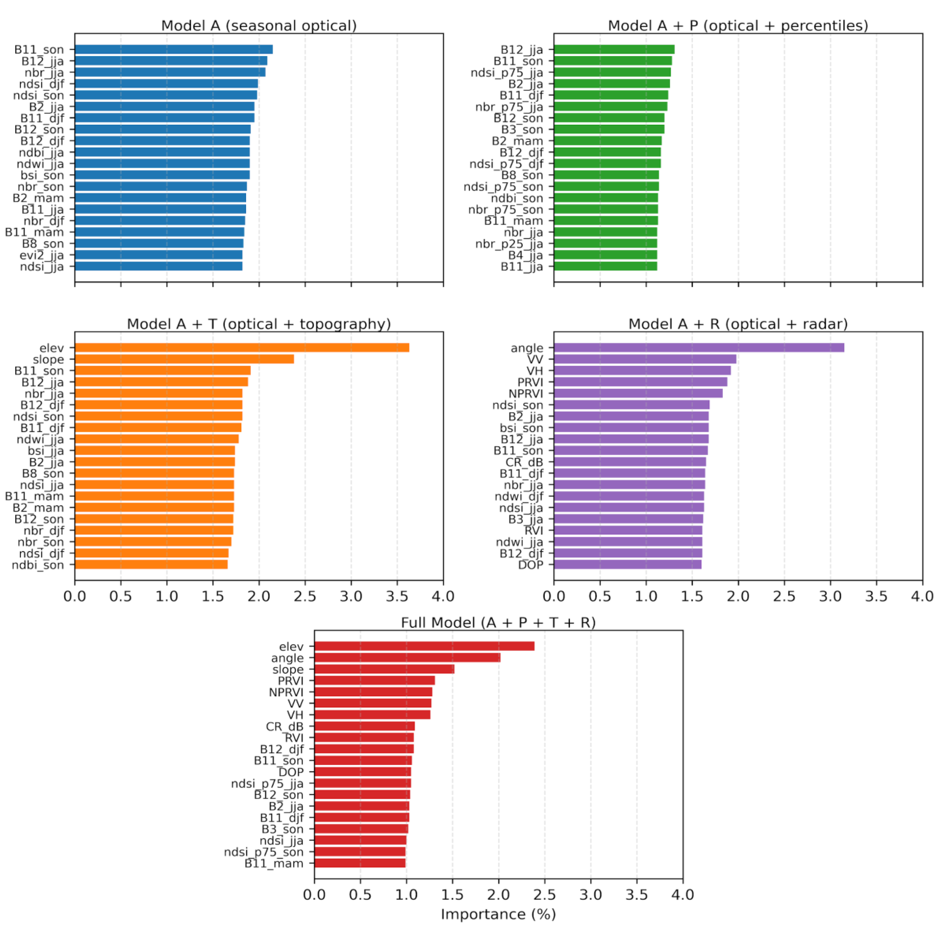
Variable importance analysis using the Random Forest classifier allowed for the identification of the most influential predictors in each model configuration and an evaluation of how their hierarchy shifts across the incremental scheme. To facilitate comparison between configurations, Figure 5 presents the 15 variables with the highest relative importance for each case, estimated using the Mean Decrease in Gini Index.
In the seasonal optical baseline model (A), the importance hierarchy is dominated by short-wave infrared (SWIR) bands, specifically B11_son and B12_jja. These are accompanied by spectral indices associated with snow, moisture, and the contrast between vegetated and non-vegetated surfaces (NDSI, NBR, NDWI, NDBI y BSI). This pattern indicates that the classification relies primarily on spectral contrasts related to surface moisture conditions, seasonal snow presence, and the differentiation of land cover states.
The incorporation of multi-temporal percentiles (A+P) maintains the SWIR bands as pillars but introduces statistical metrics of intra-annual extremes. In particular, the high percentiles of indices related to snow and surface/vegetation cover state (such as NDSI_p75 and NBR_p75) gain greater relevance. This suggests that the persistence or maximum intensity of certain events throughout the year provides critical information that complements the data contained in seasonal medians.
In the model with topography (A+T), a marked shift in the importance hierarchy is observed, with elevation and slope occupying the top-ranking positions and significantly outperforming individual spectral predictors. Although seasonal optical variables remain in the list, their relative weight decreases. This pattern confirms the foundational role of relief and the altitudinal gradient in the spatial distribution of land covers within the study area.
Analysis of the radar-integrated model (A+R) shows that the importance hierarchy is headed by the acquisition geometry variable (angle), followed by VV and VH backscatter intensities, and derived SAR indices sensitive to structure and scattering, such as PRVI and NPRVI. These variables exceed the importance of the optical bands, which remain in intermediate ranking positions. This pattern suggests that, in this configuration, the primary contribution of SAR is linked to capturing the geometric and structural information of the terrain.
Finally, in the Full model (A+P+T+R), the set of most influential variables is dominated by physical landscape descriptors, with elevation and slope among the highest-weighted predictors, alongside the acquisition geometry variable (angle). In this context, there is a prominent presence of SAR variables within the top 10, including PRVI, NPRVI, VV, VH, CR, and RVI. Optical variables appear starting from the seventh position in the ranking (e.g., B12_djf and B11_son). Taken together, this pattern highlights the integrated contribution of topographic gradients, observation geometry, and SAR descriptors in achieving the highest global performance.
For further details, the complete list of the top 20 variables for each model configuration is provided in Appendix A.
3.4. Spatial Consistency of the Mapping
The spatial distribution of land use and land cover produced by the best-performing configuration (Full model, A+P+T+R) for the entire study area is shown in Figure 6. At the basin scale, the map adequately reproduces the main ecological and land-use gradients characteristic of the region, capturing the transition from steppe and shrubland in the eastern sector, through an intermediate agricultural–forestry mosaic, to evergreen forests in the western sector, as well as the location of the main urban centers
a) Case 1: Lacustrine–steppe transition in the Lago Misterioso sector
In the reference image, the interface between native forest and forest plantations is clearly distinguishable, associated with the reddish tones of native forest during its autumn phenological phase and the more homogeneous texture and regular geometry of evergreen plantations. This pattern is consistently reproduced in the classification maps.
In the optical baseline model (A) and the A+P configuration, persistent commission errors are observed for the Urban class, reflected in low User’s Accuracy values (UA = 72.0% and 75.4%, respectively), together with an over-assignment of the Wetlands class at higher elevations, consistent with UA = 73.4% in both configurations. These confusions are visually expressed as spurious Urban and Wetlands assignments in areas where such covers are not expected according to ground reference information.
The incorporation of topographic variables (A+T) leads to a clear reduction of Wetlands at higher elevations, with an increase in UA to 81.6% and in F1 to 81.5%, consistent with the visual removal of spurious wetlands on slopes and steep terrain. In this configuration, greater spatial stability is also observed for classes such as Steppe and Bare Soil; however, this improvement does not translate into a reduction of commission errors for the Urban class, whose UA decreases to 68.8%.
The inclusion of radar information (A+R) produces a clear reduction in Urban commission errors, with UA increasing to 77.6% and F1 to 86.8%, consistent with a more accurate delineation of lacustrine–terrestrial transitions. For Wetlands, improvements are more moderate (UA = 80.4%; F1 = 79.5%).
Finally, the Full model (A+P+T+R) consolidates the observed reductions, achieving UA = 88.9% and F1 = 93.0% for the Urban class, and UA = 83.8% and F1 = 83.1% for Wetlands, while classes that were already well characterized (e.g., Water, Native Forest, and Forest Plantations) remain stable (F1 ≥ 93%). Overall, these results are reflected in enhanced spatial stability of lacustrine–terrestrial interfaces within the analyzed area.
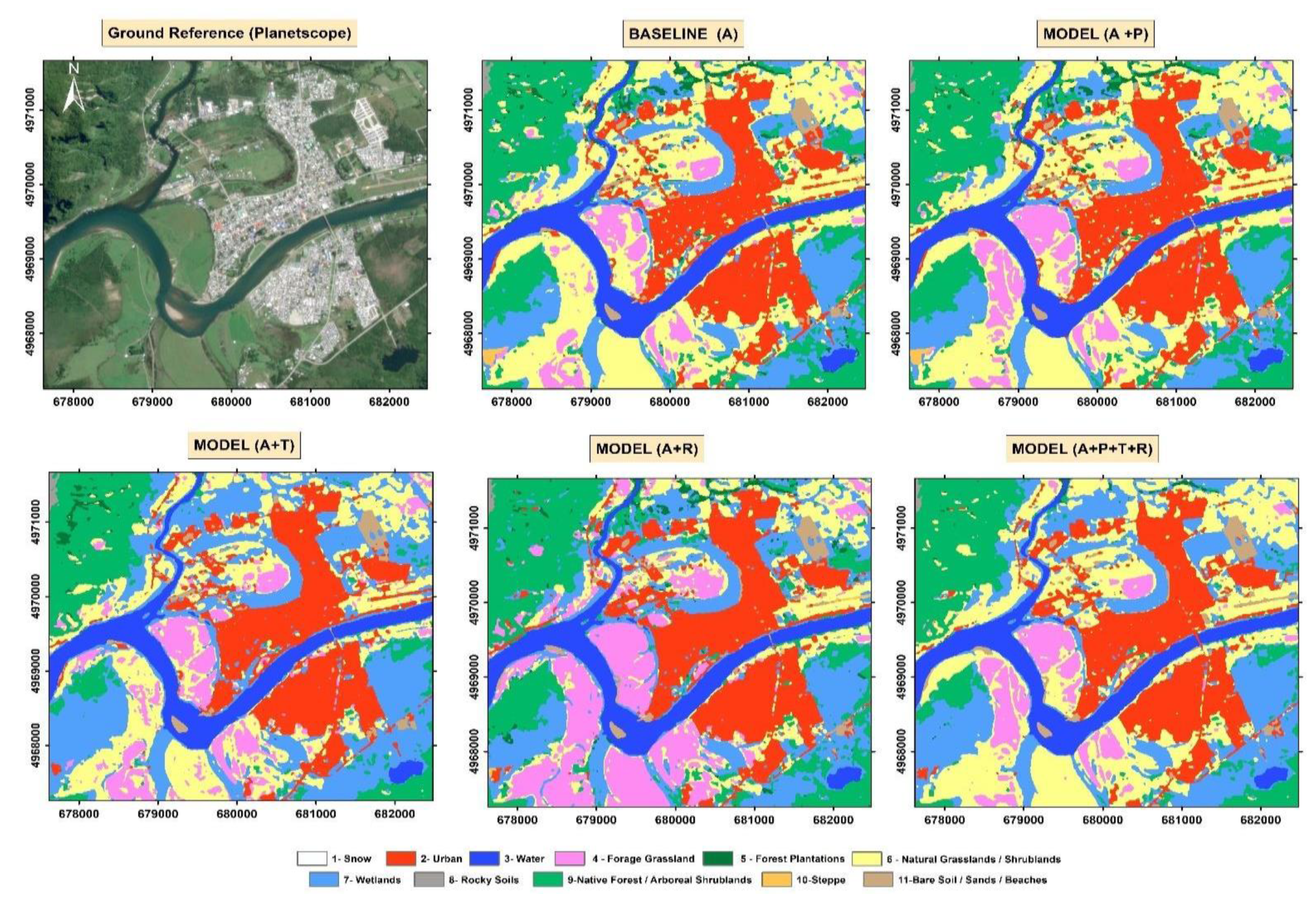
b) Case 2: Urban–fluvial environment of the city of Puerto Aysén
This case examines the spatial consistency of the mapping in a complex urban–fluvial setting characterized by compact urban areas, active alluvial plains, riparian wetlands, and bare-soil surfaces linked to fluvial bars.
In configurations A and A+P, persistent commission errors are observed for the Urban class, manifested as spurious expansion into riparian sectors and non-built surfaces, consistent with the low UA values reported (72.0% and 75.4%, respectively). These confusions are mainly concentrated along urban–fluvial interfaces and in transitions with Bare Soil/Sands and Wetlands. The incorporation of topography (A+T) contributes to greater spatial coherence of the fluvial corridor and adjacent alluvial surfaces but does not reduce Urban commission errors (UA = 68.8%), indicating that topographic information stabilizes the geomorphological context without directly discriminating urban cover.
In contrast, the A+R configuration shows a clear reduction in Urban commission errors, with UA increasing to 77.6% and F1 to 86.8%, reflected in a more precise delineation of the urban footprint. For Wetlands, improvements are moderate (UA = 80.4%; F1 = 79.5%), associated with a progressive stabilization of their spatial distribution. The Full model (A+P+T+R) consolidates these improvements, achieving the highest accuracy values for the Urban class (UA = 88.9%; F1 = 93.0%) and enhanced spatial stability along urban–riparian interfaces.
3.5. Sensitivity to the Temporal Aggregation of SAR Variables
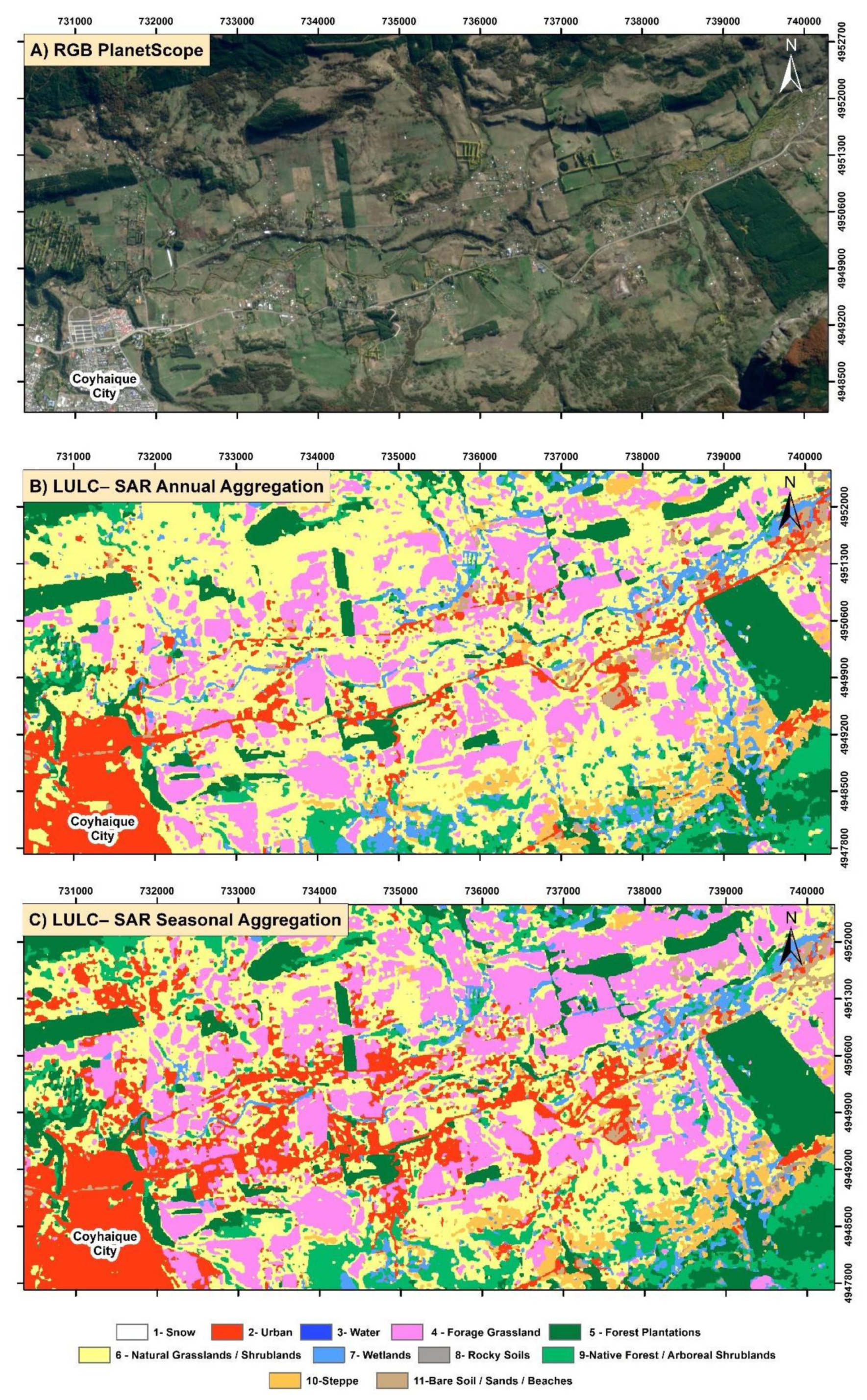
As a complementary analysis, the sensitivity of the integrated model (A+P+T+R) to the temporal aggregation scheme of SAR variables was evaluated by comparing the annual aggregation used in the main experimental design with an alternative seasonal aggregation.
From a quantitative perspective, the SAR seasonal-aggregation variant yielded additional gains in global metrics relative to the Full model with annual aggregation (OA = 92.5%; Macro-F1 = 86.0%), reaching an OA of 92.9% and a Macro-F1 of 89.5%. These values correspond to increases of +0.4 and +3.5 percentage points, respectively.
However, qualitative inspection of spatial consistency reveals contrasting behavior. Figure 7 illustrates this effect in the urban–periurban environment of Coyhaique, comparing the optical reference (Figure 7A) with the Full model using annual SAR aggregation (Figure 7B) and its seasonal-aggregation variant (Figure 7C). While annual aggregation preserves a compact urban delineation that is consistent with the reference, seasonal aggregation induces spurious expansion of the Urban class into rural and periurban areas.
Figure 8.
Spatial comparison between the reference image (RGB composite acquired on 08 April 2021) and the classification maps corresponding to configurations A, A+P, A+T, A+R, and Full (A+P+T+R) in the urban–fluvial environment of the city of Puerto Aysén, characterized by the coexistence of compact urban areas, active alluvial plains, riparian wetlands, and bare-soil surfaces associated with fluvial bars.
A similar, though less pronounced, pattern is observed for Forage Grasslands, which exhibit increased spatial fragmentation under seasonal aggregation.
4. Discussion
The results demonstrate that the synergy between multi-seasonal optical data, multi-temporal SAR observations, and topographic variables significantly enhances LULC classification in complex Andean ecosystems. The performance of the Full model (OA: 92.5%; Macro-F1: 86.0%) confirms that multisensor integration is not merely additive but genuinely complementary, particularly in mitigating the effects of class imbalance (Table 4).
4.1. Multisensor Synergy and Model Performance
The integration of optical, radar, and topographic data proved decisive for accurate LULC mapping within the complex orography of the Aysén basin. Overall Accuracy increased progressively from 89.2% in the optical baseline model to 92.5% in the Full model. This performance gain is especially relevant when contrasted with national-scale mapping efforts in Chile, where a systematic decline in accuracy toward austral latitudes has been reported due to persistent cloud cover and complex terrain [13]. By surpassing these previously reported regional standards, the present results demonstrate that the complementarity of multiple data domains can resolve ambiguities that are otherwise intractable when relying on a single sensor. Moreover, the observed gain of +5.5 percentage points in Macro-F1 is consistent with previous studies conducted in heterogeneous landscapes, which have shown that the fusion of optical and radar information systematically improves the discrimination of complex land-cover classes compared to single-source approaches [54,55].
Although optical data (Sentinel-2) effectively captured phenological variability, as reflected by the dominance of SWIR bands (B11, B12) and snow- and vegetation-related indices in the baseline model, this information alone was insufficient to differentiate classes with similar spectral responses but distinct geometric or structural configurations. In this context, the incorporation of Sentinel-1 SAR backscatter (A+R configuration) yielded the largest marginal performance gain (+2.5% in OA). This improvement is attributed to the ability of radar data to introduce descriptors sensitive to surface roughness and three-dimensional canopy organization, thereby facilitating the separation of structurally complex classes such as urban areas, bare soil, and shrublands [55].
4.2. The role of Topography and SAR in Structural Discrimination
Our findings highlight topography as a key structuring factor of the landscape. The dominance of elevation and slope in the variable-importance ranking (Figure 5) is consistent with the environmental gradients of the Aysén River Basin, where altitude governs wetland distribution and the upper treeline. In this context, the inclusion of topographic variables (A+T) effectively corrected commission errors associated with wetlands on steep slopes (Figure 7), a recurrent issue in classifications based exclusively on optical information, where topographic shadows or surfaces with high soil moisture can mimic wetland spectral signatures [56].
However, the results also indicate that topography, while a robust predictor for natural land covers, is insufficient for urban discrimination in the complex environments of Patagonia. Under the A+T configuration, relief variables introduced a systematic bias, reducing the User’s Accuracy (UA) of the Urban class from 72.0% to 68.8% (Figure 4). This limitation is consistent with findings from national-scale mapping efforts in Chile, where austral topographic complexity hampers land-cover separation even when digital elevation models and multi-temporal optical data are integrated [13]. This behavior can be explained by geographic covariance, whereby low slope acts as a positional predictor of settlements. In the Aysén River Basin, urban centers such as Puerto Aysén and Coyhaique are located on fluvial terraces and alluvial plains, sharing this geomorphological niche with forage grasslands and sand bars. This ambiguity underscores that topographic variables operate as environmental proxies but lack the physical discriminatory power required to separate spectrally similar classes within the same altitudinal domain [54].
Resolution of this bias is achieved through the incorporation of Sentinel-1 SAR signals (A+R). Radar sensitivity to surface roughness and double-bounce scattering mechanisms enables effective separation of built infrastructure from natural substrates, as documented in previous SAR–optical fusion studies for urban mapping [57,58]. Furthermore, the high importance of the acquisition geometry variable (angle) in the Full model indicates effective integration of the sensor–terrain relationship, allowing compensation for radiometric distortions inherent to SAR acquisition in mountainous terrain [59].
4.3. Spatial Consistency Versus Statistical Metrics
The sensitivity analysis of SAR temporal aggregation revealed a critical discrepancy between statistical performance metrics and cartographic quality. Although the seasonal-SAR variant of the Full model (A+P+T+R) numerically outperformed the annual aggregation (Macro-F1: 89.5% vs. 86.0%), visual inspection demonstrated that this metric gain masked a degradation in spatial coherence through the introduction of significant artifacts, such as spurious urban expansion (Figure 9). This behavior suggests that high-frequency SAR variability, associated with management dynamics in forage grasslands and seasonal changes in soil moisture, can induce transient increases in backscatter that mimic the high returns typically associated with urban infrastructure. Such radiometric ambiguity between built-up surfaces and natural substrates with high surface roughness or rocky components is a well-documented challenge in Sentinel-1–based mapping, particularly in heterogeneous and topographically complex environments where distinct land covers may produce similar signal response [59].
In this context, the use of seasonal aggregations increases the likelihood that the classifier incorporates transient radiometric variability linked to short-term environmental conditions rather than to the permanent structure of land covers. Methodological studies on SAR preprocessing have emphasized that decisions regarding temporal aggregation and radiometric stabilization directly affect the robustness of derived products and the suppression of spurious artifacts [60]. By contrast, the annual median composite acted as a robust temporal filter, smoothing transient noise and prioritizing the geographic consistency of permanent structures over marginal gains in global statistical metrics.
4.4. Persistent Challenges in Natural Grasslands
The Natural Grasslands/Shrublands class represented the primary challenge within the classification scheme, exhibiting the lowest performance in the Full model (F1 = 70.4%). In the seasonal optical baseline model, this class showed systematic overestimation, associated with its high spectral and phenological similarity to forage grasslands, which limits discrimination based solely on optical reflectance [61].
The incorporation of topographic and radar information reduced commission errors, increasing User’s Accuracy (UA = 67.3%). However, this improvement was accompanied by reduced sensitivity, reflecting a characteristic trade-off for transitional land covers with high internal heterogeneity. From a biophysical perspective, this limitation can be explained by phenological overlap in the optical domain [62] and by the limited ability of C-band SAR to resolve fine-scale structural differences. At the pixel scale, the volumetric scattering response of sparse shrublands is comparable to that generated by dense, managed grasslands [56].
In this context, surpassing the current accuracy threshold will likely require future approaches that explicitly incorporate spatial context, such as object-based image analysis (GEOBIA) or deep learning architectures. These methods have demonstrated potential for addressing persistent confusion among land-cover classes with similar physical signatures [56,63].
Figure 9.
Sensitivity of the Full model to SAR temporal aggregation at the urban–periurban interface of Coyhaique. (A) Optical reference image from PlanetScope (RGB composite acquired on 08 April 2021). (B) Full model with annual SAR aggregation, showing a compact and spatially coherent urban delineation. (C) Full model variant with seasonal SAR aggregation, characterized by spurious urban expansion and increased spatial fragmentation.
5. Conclusions
The implemented ablation design demonstrated that multisensor fusion is indispensable for overcoming the limitations of optical remote sensing in complex Andean landscapes. Beyond improving global performance, this approach allowed for the decoupling and quantification of contributions from complementary information domains. While the central tendency baseline proved insufficient for capturing compositional heterogeneity (Macro-F1 = 80.5%), the inclusion of phenological metrics (P) refined vegetation discrimination, and the subsequent integration of topographic (T) and radar (R) variables generated critical, non-redundant gains (+3.8 points each), acting as geomorphological filters and structural descriptors. The integrated model (A+P+T+R) maximized global performance (OA = 92.5%; Macro-F1 = 86.0%), validating the hypotheses regarding the necessary complementarity between phenological dynamics (H1), physical structure (H2), and topographic landscape context (H3).
Methodologically, this study cautions against optimizing statistical metrics at the expense of the spatial plausibility of cartographic products. It was shown that although seasonal SAR data aggregation improved numerical metrics, it introduced noise and geometric artifacts; in contrast, annual composites operated as robust temporal regularizers, prioritizing cartographic coherence over marginal metric gains. Nonetheless, challenges persist in transitional classes such as Grasslands/Shrublands (F1 ≈ 70%), suggesting a future need to incorporate explicit spatial context (e.g., Deep Learning or GEOBIA) to resolve fine-scale ambiguities. From an operational perspective, the developed workflow based entirely on open data from the Copernicus program and cloud-based processing constitutes a cost-effective and scalable solution for the systematic production of LULC maps in vast and inaccessible regions. This approach is directly transferable to land management agencies, enabling frequent updates of land cover data, a key input for watershed management, fire monitoring, and planning under climate change scenarios.
Author Contributions
Conceptualization, methodology, investigation, formal analysis, software, resources, data curation, validation, visualization, writing—original draft preparation, writing—review and editing, K.E.; J.V; G.O; data curation, visualization, writing—review and editing, V.S.
Funding
Funded by the European Union under grant agreement No.101131859. Views and opinions expressed are however those of the author(s) only and do not necessarily reflect those of the European Union or EUSPA. Neither the European Union nor the granting authority can be held responsible for them.
Acknowledgments
The authors would like to thank Planet Labs for providing PlanetScope data via the E&R Program to KE.:.
Conflicts of Interest
Declare conflicts of interest or state “The authors declare no conflicts of interest.” Authors must identify and declare any personal circumstances or interest that may be perceived as inappropriately influencing the representation or interpretation of reported research results. Any role of the funders in the design of the study; in the collection, analyses or interpretation of data; in the writing of the manuscript; or in the decision to publish the results must be declared in this section. If there is no role, please state “The funders had no role in the design of the study; in the collection, analyses, or interpretation of data; in the writing of the manuscript; or in the decision to publish the results”.
Appendix A
Figure A1.
Ranking of the 20 most influential variables for each classification model configuration (A, A+P, A+T, A+R, and Full), based on the Mean Decrease in Gini Index.
Figure A1.
Ranking of the 20 most influential variables for each classification model configuration (A, A+P, A+T, A+R, and Full), based on the Mean Decrease in Gini Index.
References
- Shukla, P.R.; Skeg, J.; Buendia, E.C.; Masson-Delmotte, V.; Pörtner, H.-O.; Roberts, D.; Zhai, P.; Slade, R.; Connors, S.; Van Diemen, S. Climate Change and Land: an IPCC special report on climate change, desertification, land degradation, sustainable land management, food security, and greenhouse gas fluxes in terrestrial ecosystems. 2019. [Google Scholar]
- Velastegui-Montoya, A.; Montalván-Burbano, N.; Carrión-Mero, P.; Rivera-Torres, H.; Sadeck, L.; Adami, M. Google Earth Engine: a global analysis and future trends. Remote Sensing 2023, 15, 3675. [Google Scholar] [CrossRef]
- Amin, G.; Imtiaz, I.; Haroon, E.; Saqib, N.u.; Shahzad, M.I.; Nazeer, M. Assessment of machine learning algorithms for land cover classification in a complex mountainous landscape. Journal of Geovisualization and Spatial Analysis 2024, 8, 34. [Google Scholar] [CrossRef]
- Talukdar, S.; Singha, P.; Mahato, S.; Pal, S.; Liou, Y.-A.; Rahman, A. Land-use land-cover classification by machine learning classifiers for satellite observations—A review. Remote sensing 2020, 12, 1135. [Google Scholar] [CrossRef]
- Belcore, E.; Piras, M.; Wozniak, E. Specific alpine environment land cover classification methodology: Google earth engine processing for sentinel-2 data. The International Archives of the Photogrammetry, Remote Sensing and Spatial Information Sciences 2020, 43, 663–670. [Google Scholar] [CrossRef]
- Argandoña-Castro, F.; Peña-Cortés, F. A Systematic Review of Developments in Farmland Cover in Chile: Dynamics and Implications for a Sustainable Future in Land Use. Sustainability 2025, 17, 3905. [Google Scholar] [CrossRef]
- Bizama, G.; Torrejón, F.; Aguayo, M.; Muñoz, M.D.; Echeverría, C.; Urrutia, R. Pérdida y fragmentación del bosque nativo en la cuenca del río Aysén (Patagonia-Chile) durante el siglo XX. Revista de Geografía Norte Grande 2011, 125–138. [Google Scholar] [CrossRef]
- Castilla, J.C.; Armesto, J.J.; Martínez-Harms, M.J. Conservación en la Patagonia chilena: evaluación del conocimiento, oportunidades y desafíos; Ediciones UC, 2021. [Google Scholar]
- Buchhorn, M.; Lesiv, M.; Tsendbazar, N.-E.; Herold, M.; Bertels, L.; Smets, B. Copernicus global land cover layers—collection 2. Remote Sensing 2020, 12, 1044. [Google Scholar] [CrossRef]
- CONAF, C.N.F. Catastro de los recursos vegetacionales y uso de la tierra de la Región de Aysén del General Carlos Ibáñez del Campo, actualización 2020–2022. 2024. [Google Scholar]
- MapBiomas Chile. Algorithm Theoretical Basis Document (ATBD): Colección 1.0. Available online: https://chile.mapbiomas.org/wp-content/uploads/sites/13/2024/04/ATBD_Chile-Coll-1.pdf (accessed on.
- Azzari, G.; Lobell, D. Landsat-based classification in the cloud: An opportunity for a paradigm shift in land cover monitoring. Remote Sensing of Environment 2017, 202, 64–74. [Google Scholar] [CrossRef]
- Zhao, Y.; Feng, D.; Yu, L.; Wang, X.; Chen, Y.; Bai, Y.; Hernández, H.J.; Galleguillos, M.; Estades, C.; Biging, G.S. Detailed dynamic land cover mapping of Chile: Accuracy improvement by integrating multi-temporal data. Remote Sensing of Environment 2016, 183, 170–185. [Google Scholar] [CrossRef]
- Clerici, N.; Valbuena Calderón, C.A.; Posada, J.M. Fusion of Sentinel-1A and Sentinel-2A data for land cover mapping: a case study in the lower Magdalena region, Colombia. Journal of Maps 2017, 13, 718–726. [Google Scholar] [CrossRef]
- Hethcoat, M.G.; Edwards, D.P.; Carreiras, J.M.; Bryant, R.G.; Franca, F.M.; Quegan, S. A machine learning approach to map tropical selective logging. Remote sensing of environment 2019, 221, 569–582. [Google Scholar] [CrossRef]
- Torres-Gómez, M.; Delgado, L.E.; Marín, V.H.; Bustamante, R.O. Estructura del paisaje a lo largo de gradientes urbano-rurales en la cuenca del río Aisén (Región de Aisén, Chile). Revista chilena de historia natural 2009, 82, 73–82. [Google Scholar] [CrossRef]
- Pérez, T.; Mattar, C.; Fuster, R. Decrease in snow cover over the Aysén river catchment in Patagonia, Chile. Water 2018, 10, 619. [Google Scholar] [CrossRef]
- Sade, K.; Pérez, L. El impacto humano sobre el paisaje arqueológico en la Cuenca del Río Aysén. In Proceedings of the ctas del VIII Congreso de Historia Social y Política de la Patagonia argentino chilena, Rawson 2009. pp. 266–274., 2011.
- Gorelick, N.; Hancher, M.; Dixon, M.; Ilyushchenko, S.; Thau, D.; Moore, R. Google Earth Engine: Planetary-scale geospatial analysis for everyone. Remote sensing of Environment 2017, 202, 18–27. [Google Scholar] [CrossRef]
- Louis, J.; Pflug, B.; Main-Knorn, M.; Debaecker, V.; Mueller-Wilm, U.; Iannone, R.Q.; Cadau, E.G.; Boccia, V.; Gascon, F. Sentinel-2 global surface reflectance level-2A product generated with Sen2Cor. In Proceedings of the IGARSS 2019-2019 IEEE International Geoscience and Remote Sensing Symposium, 2019; pp. 8522–8525.
- Phiri, D.; Simwanda, M.; Salekin, S.; Nyirenda, V.R.; Murayama, Y.; Ranagalage, M. Sentinel-2 data for land cover/use mapping: A review. Remote sensing 2020, 12, 2291. [Google Scholar] [CrossRef]
- Hall, D.K.; Riggs, G.A. Normalized-difference snow index (NDSI). Encyclopedia of snow, ice and glaciers 2010. [Google Scholar]
- Marzi, D.; Sorriso, A.; Gamba, P. Automatic wide area land cover mapping using Sentinel-1 multitemporal data. Frontiers in Remote Sensing 2023, 4, 1148328. [Google Scholar] [CrossRef]
- Schulz, D.; Yin, H.; Tischbein, B.; Verleysdonk, S.; Adamou, R.; Kumar, N. Land use mapping using Sentinel-1 and Sentinel-2 time series in a heterogeneous landscape in Niger, Sahel. ISPRS Journal of Photogrammetry and Remote Sensing 2021, 178, 97–111. [Google Scholar] [CrossRef]
- Farr, T.G.; Rosen, P.A.; Caro, E.; Crippen, R.; Duren, R.; Hensley, S.; Kobrick, M.; Paller, M.; Rodriguez, E.; Roth, L. The shuttle radar topography mission. Reviews of geophysics 2007, 45. [Google Scholar] [CrossRef]
- Uuemaa, E.; Ahi, S.; Montibeller, B.; Muru, M.; Kmoch, A. Vertical accuracy of freely available global digital elevation models (ASTER, AW3D30, MERIT, TanDEM-X, SRTM, and NASADEM). Remote Sensing 2020, 12, 3482. [Google Scholar] [CrossRef]
- Jpl, N. NASA Shuttle Radar Topography Mission Global 3 arc second number NetCDF. NASA EOSDIS Land Processes Distributed Active Archive Center (DAAC) data set 2013, SRTMGL3_NUMNC. 003.
- Olofsson, P.; Foody, G.M.; Stehman, S.V.; Woodcock, C.E. Making better use of accuracy data in land change studies: Estimating accuracy and area and quantifying uncertainty using stratified estimation. Remote sensing of environment 2013, 129, 122–131. [Google Scholar] [CrossRef]
- Hollstein, A.; Segl, K.; Guanter, L.; Brell, M.; Enesco, M. Ready-to-use methods for the detection of clouds, cirrus, snow, shadow, water and clear sky pixels in Sentinel-2 MSI images. Remote Sensing 2016, 8, 666. [Google Scholar] [CrossRef]
- Rifai, M. Integration of Cloud Score+ with Sentinel-2 Harmonized for land use and land cover classification using machine learning algorithms. In Proceedings of the IOP Conference Series: Earth and Environmental Science, 2024; p. 012039. [Google Scholar]
- Flood, N. Seasonal composite Landsat TM/ETM+ images using the medoid (a multi-dimensional median). Remote Sensing 2013, 5, 6481–6500. [Google Scholar] [CrossRef]
- Griffiths, P.; Hostert, P.; Gruebner, O.; van der Linden, S. Mapping megacity growth with multi-sensor data. Remote sensing of Environment 2010, 114, 426–439. [Google Scholar] [CrossRef]
- Phan, T.N.; Kuch, V.; Lehnert, L.W. Land cover classification using Google Earth Engine and random forest classifier—The role of image composition. Remote Sensing 2020, 12, 2411. [Google Scholar] [CrossRef]
- Griffiths, P.; van der Linden, S.; Kuemmerle, T.; Hostert, P. A pixel-based Landsat compositing algorithm for large area land cover mapping. IEEE Journal of Selected Topics in Applied Earth Observations and Remote Sensing 2013, 6, 2088–2101. [Google Scholar] [CrossRef]
- Zanaga, D.; Van De Kerchove, R.; Daems, D.; De Keersmaecker, W.; Brockmann, C.; Kirches, G.; Wevers, J.; Cartus, O.; Santoro, M.; Fritz, S. ESA WorldCover 10 m 2021 v200. 2022. [Google Scholar]
- Rouse Jr, J.W.; Haas, R.H.; Schell, J.; Deering, D. Monitoring the vernal advancement and retrogradation (green wave effect) of natural vegetation; 1973.
- Jiang, Z.; Huete, A.R.; Didan, K.; Miura, T. Development of a two-band enhanced vegetation index without a blue band. Remote sensing of Environment 2008, 112, 3833–3845. [Google Scholar] [CrossRef]
- Huete, A.R. A soil-adjusted vegetation index (SAVI). Remote sensing of environment 1988, 25, 295–309. [Google Scholar] [CrossRef]
- McFeeters, S.K. The use of the Normalized Difference Water Index (NDWI) in the delineation of open water features. International journal of remote sensing 1996, 17, 1425–1432. [Google Scholar] [CrossRef]
- Hall, D.K.; Riggs, G.A.; Salomonson, V.V. Development of methods for mapping global snow cover using moderate resolution imaging spectroradiometer data. Remote sensing of Environment 1995, 54, 127–140. [Google Scholar] [CrossRef]
- Key, C.H.; Benson, N.C. Landscape assessment (LA). In: Lutes, Duncan C.; Keane, Robert E.; Caratti, John F.; Key, Carl H.; Benson, Nathan C.; Sutherland, Steve; Gangi, Larry J. 2006. FIREMON: Fire effects monitoring and inventory system. Gen. Tech. Rep. RMRS-GTR-164-CD. Fort Collins, CO: US Department of Agriculture, Forest Service, Rocky Mountain Research Station. p. LA-1-55 2006, 164.
- Zha, Y.; Gao, J.; Ni, S. Use of normalized difference built-up index in automatically mapping urban areas from TM imagery. International journal of remote sensing 2003, 24, 583–594. [Google Scholar] [CrossRef]
- Rikimaru, A.; Roy, P.S.; Miyatake, S. Tropical forest cover density mapping. Tropical ecology 2002, 43, 39–47. [Google Scholar]
- Burrough, P.A. Principles of geographical. Information systems for land resource assessment; Clarendon Press: Oxford, 1986. [Google Scholar]
- Beers, T.W.; Dress, P.E.; Wensel, L.C. Notes and observations: aspect transformation in site productivity research. Journal of Forestry 1966, 64, 691–692. [Google Scholar] [CrossRef]
- Torres, R.; Snoeij, P.; Geudtner, D.; Bibby, D.; Davidson, M.; Attema, E.; Potin, P.; Rommen, B.; Floury, N.; Brown, M. GMES Sentinel-1 mission. Remote sensing of environment 2012, 120, 9–24. [Google Scholar] [CrossRef]
- Lee, J.-S.; Pottier, E. Polarimetric radar imaging: from basics to applications; CRC press, 2017. [Google Scholar]
- Chang, J.G.; Kraatz, S.; Anderson, M.; Gao, F. Enhanced polarimetric radar vegetation index and integration with optical index for biomass estimation in grazing lands across the contiguous United States. Remote Sensing 2024, 16, 4476. [Google Scholar] [CrossRef]
- Mandal, D.; Kumar, V.; Ratha, D.; Dey, S.; Bhattacharya, A.; Lopez-Sanchez, J.M.; McNairn, H.; Rao, Y.S. Dual polarimetric radar vegetation index for crop growth monitoring using sentinel-1 SAR data. Remote Sensing of Environment 2020, 247, 111954. [Google Scholar] [CrossRef]
- Maxwell, A.E.; Warner, T.A.; Fang, F. Implementation of machine-learning classification in remote sensing: An applied review. International journal of remote sensing 2018, 39, 2784–2817. [Google Scholar] [CrossRef]
- Belgiu, M.; Drăguţ, L. Random forest in remote sensing: A review of applications and future directions. ISPRS journal of photogrammetry and remote sensing 2016, 114, 24–31. [Google Scholar] [CrossRef]
- Foody, G.M. Explaining the unsuitability of the kappa coefficient in the assessment and comparison of the accuracy of thematic maps obtained by image classification. Remote sensing of environment 2020, 239, 111630. [Google Scholar] [CrossRef]
- Farhadpour, S.; Warner, T.A.; Maxwell, A.E. Selecting and interpreting multiclass loss and accuracy assessment metrics for classifications with class imbalance: Guidance and best practices. Remote Sensing 2024, 16, 533. [Google Scholar] [CrossRef]
- Joshi, N.; Baumann, M.; Ehammer, A.; Fensholt, R.; Grogan, K.; Hostert, P.; Jepsen, M.R.; Kuemmerle, T.; Meyfroidt, P.; Mitchard, E.T. A review of the application of optical and radar remote sensing data fusion to land use mapping and monitoring. Remote Sensing 2016, 8, 70. [Google Scholar] [CrossRef]
- Steinhausen, M.J.; Wagner, P.D.; Narasimhan, B.; Waske, B. Combining Sentinel-1 and Sentinel-2 data for improved land use and land cover mapping of monsoon regions. International journal of applied earth observation and geoinformation 2018, 73, 595–604. [Google Scholar] [CrossRef]
- Tassi, A.; Vizzari, M. Object-oriented lulc classification in google earth engine combining snic, glcm, and machine learning algorithms. Remote Sensing 2020, 12, 3776. [Google Scholar] [CrossRef]
- Carrasco, L.; O’Neil, A.W.; Morton, R.D.; Rowland, C.S. Evaluating combinations of temporally aggregated Sentinel-1, Sentinel-2 and Landsat 8 for land cover mapping with Google Earth Engine. Remote Sensing 2019, 11, 288. [Google Scholar] [CrossRef]
- Vizzari, M. PlanetScope, Sentinel-2, and Sentinel-1 data integration for object-based land cover classification in Google Earth Engine. Remote Sensing 2022, 14, 2628. [Google Scholar] [CrossRef]
- Small, D. Flattening gamma: Radiometric terrain correction for SAR imagery. IEEE Transactions on Geoscience and Remote Sensing 2011, 49, 3081–3093. [Google Scholar] [CrossRef]
- Mullissa, A.; Vollrath, A.; Odongo-Braun, C.; Slagter, B.; Balling, J.; Gou, Y.; Gorelick, N.; Reiche, J. Sentinel-1 sar backscatter analysis ready data preparation in google earth engine. Remote Sensing 2021, 13, 1954. [Google Scholar] [CrossRef]
- Fassnacht, F.E.; Latifi, H.; Stereńczak, K.; Modzelewska, A.; Lefsky, M.; Waser, L.T.; Straub, C.; Ghosh, A. Review of studies on tree species classification from remotely sensed data. Remote sensing of environment 2016, 186, 64–87. [Google Scholar] [CrossRef]
- Griffiths, P.; Müller, D.; Kuemmerle, T.; Hostert, P. Agricultural land change in the Carpathian ecoregion after the breakdown of socialism and expansion of the European Union. Environmental Research Letters 2013, 8, 045024. [Google Scholar] [CrossRef]
- Ma, L.; Liu, Y.; Zhang, X.; Ye, Y.; Yin, G.; Johnson, B.A. Deep learning in remote sensing applications: A meta-analysis and review. ISPRS journal of photogrammetry and remote sensing 2019, 152, 166–177. [Google Scholar] [CrossRef]
Figure 1.
Location of the study area in southern Chile. (A) Regional context showing the Aysén Region of Chile highlighted in red along the Pacific coast. (B) Administrative and geographic context of the study basin within the Aysén Region. (C) Topographic overview of the study basin, including elevation, the main subantarctic river network, and urban areas.
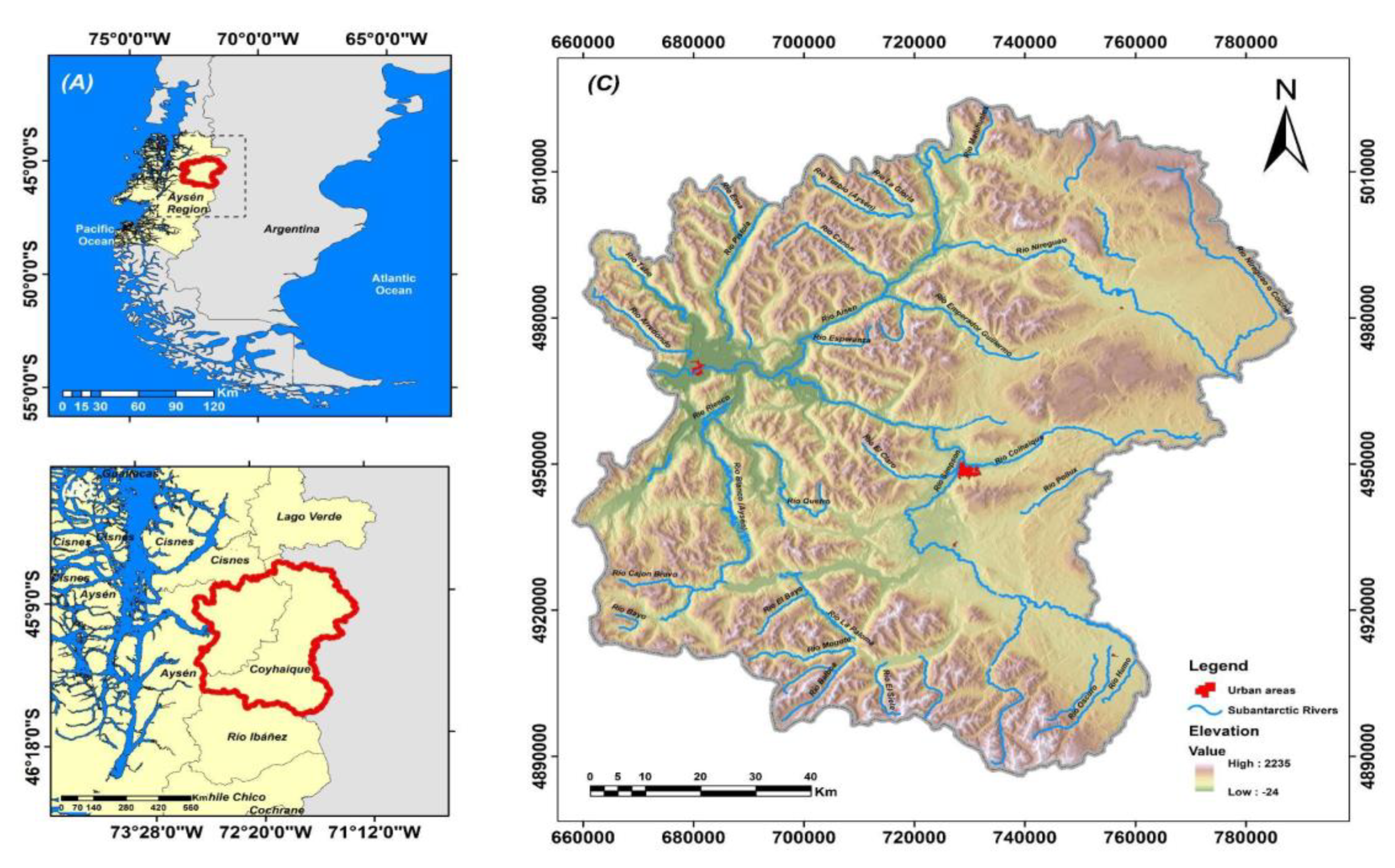
Figure 2.
Workflow for LULC classification using Random Forest and block-wise variable evaluation (optical A, percentiles P, topography T, and radar R) in the Aysén River Basin.
Figure 2.
Workflow for LULC classification using Random Forest and block-wise variable evaluation (optical A, percentiles P, topography T, and radar R) in the Aysén River Basin.
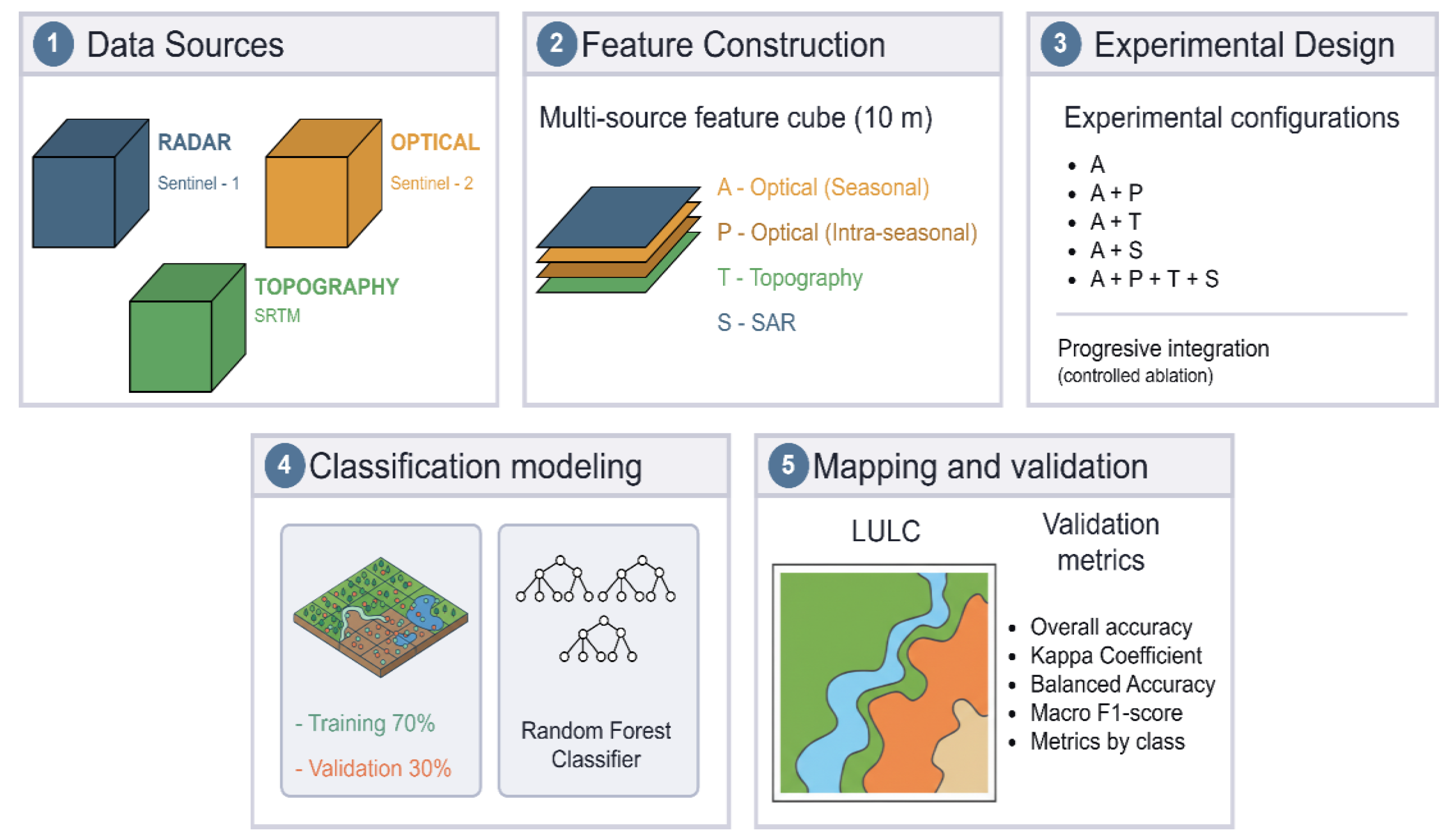
Figure 3.
Performance gains relative to the optical baseline model (A) for the different experimental configurations. Bars represent improvements in Overall Accuracy (OA), Balanced Accuracy (BA), and Macro-F1 score.
Figure 3.
Performance gains relative to the optical baseline model (A) for the different experimental configurations. Bars represent improvements in Overall Accuracy (OA), Balanced Accuracy (BA), and Macro-F1 score.
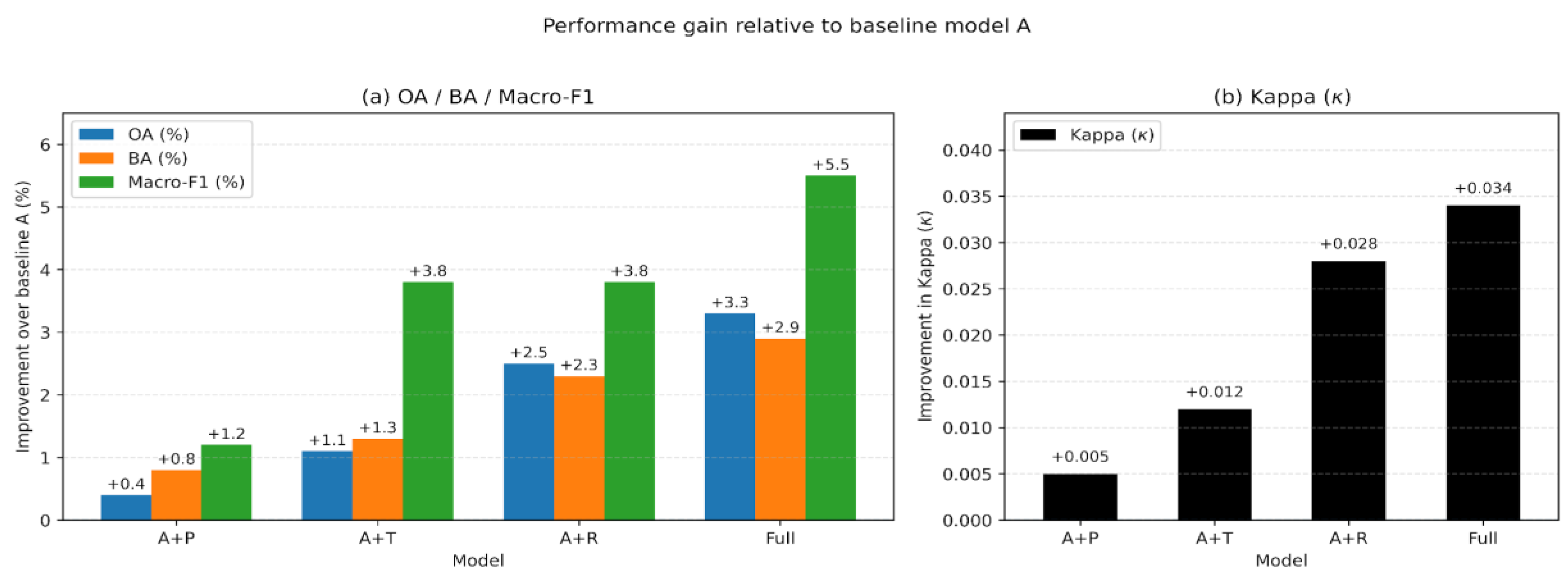
Figure 4.
Heatmap of accuracy metrics (Producer’s Accuracy—PA, User’s Accuracy—UA, and F1 score) by land-cover class and evaluated model (A, A+P, A+T, A+R, and Full).
Figure 4.
Heatmap of accuracy metrics (Producer’s Accuracy—PA, User’s Accuracy—UA, and F1 score) by land-cover class and evaluated model (A, A+P, A+T, A+R, and Full).
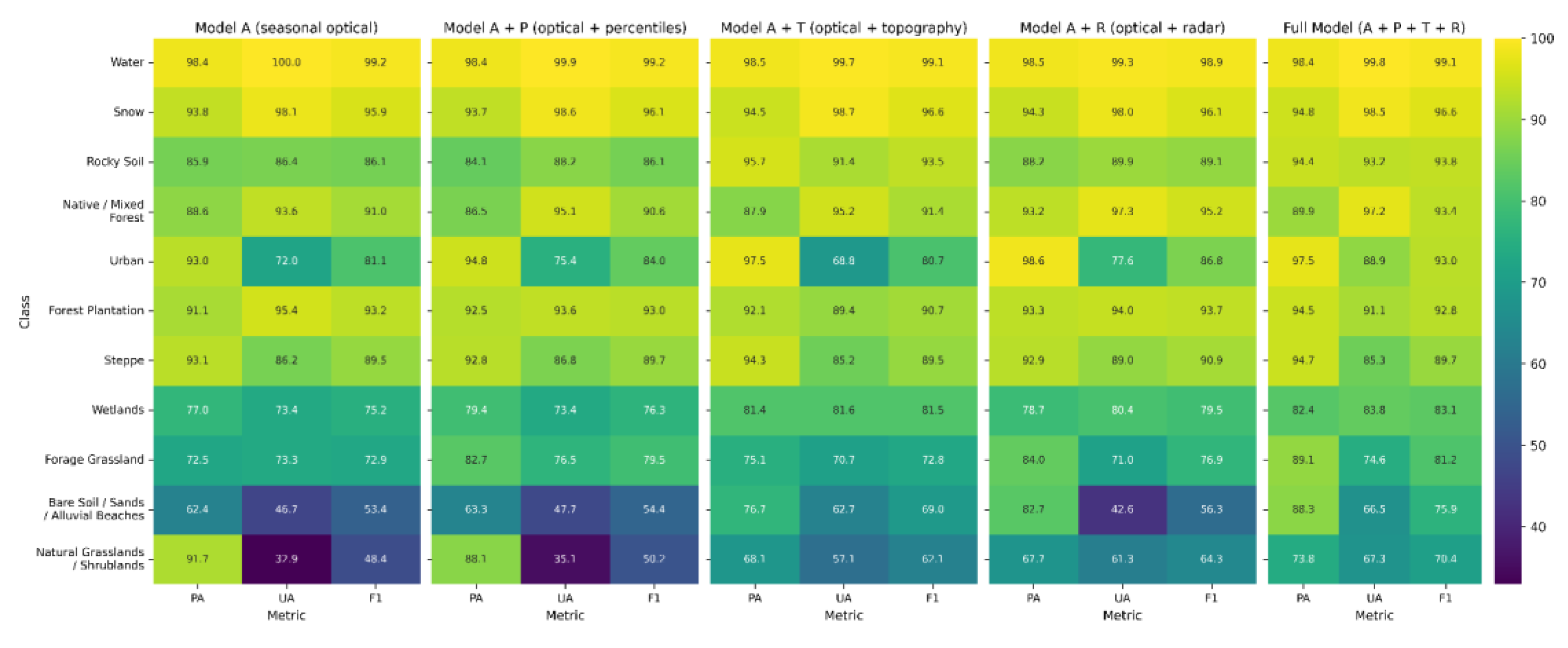
Figure 5.
Ranking of the 15 most influential variables for each classification model configuration (A, A+P, A+T, A+R, and Full), based on the Mean Decrease in Gini Index.
Figure 5.
Ranking of the 15 most influential variables for each classification model configuration (A, A+P, A+T, A+R, and Full), based on the Mean Decrease in Gini Index.
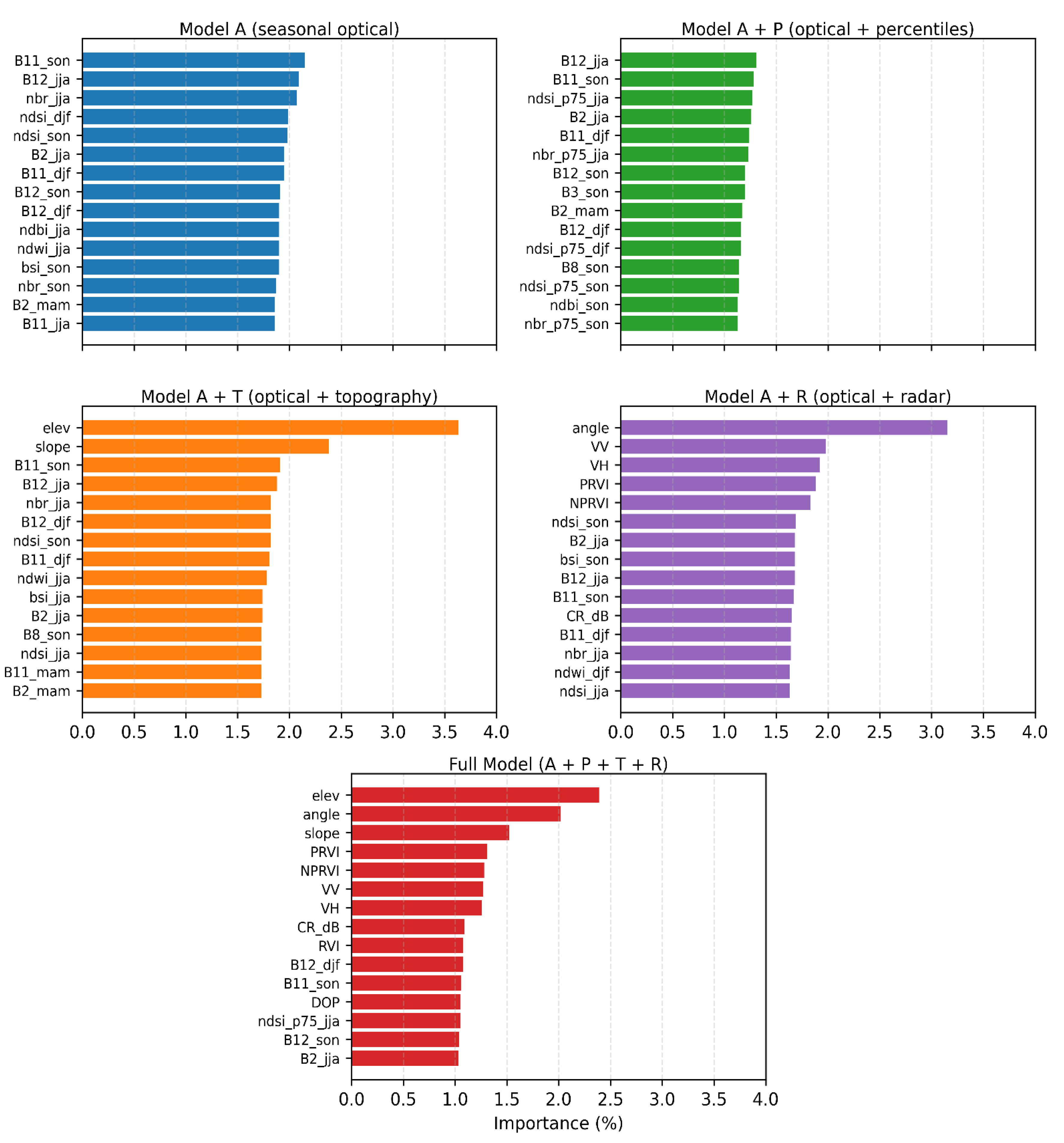
Figure 6.
Spatial distribution of land use and land cover (LULC, 2021) in the Aysén River Basin derived from the best-performing configuration (Full model, A+P+T+R).
Figure 6.
Spatial distribution of land use and land cover (LULC, 2021) in the Aysén River Basin derived from the best-performing configuration (Full model, A+P+T+R).
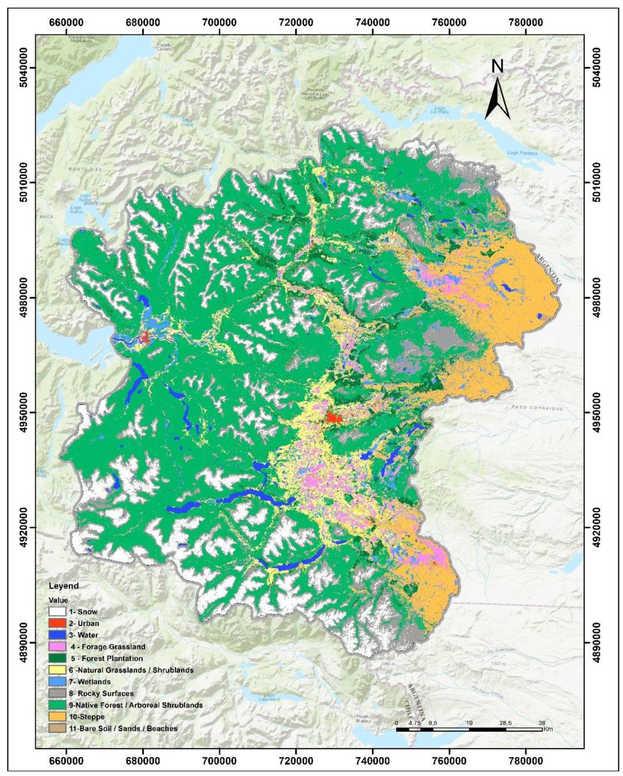
Figure 7.
Spatial comparison between the reference image (RGB composite acquired on 08 April 2021) and the classification maps corresponding to configurations A, A+P, A+T, A+R, and Full (A+P+T+R) in the Lago Misterioso sector, characterized by a highly heterogeneous lacustrine–terrestrial mosaic (wetlands, steppe, native forest, and forest plantations).
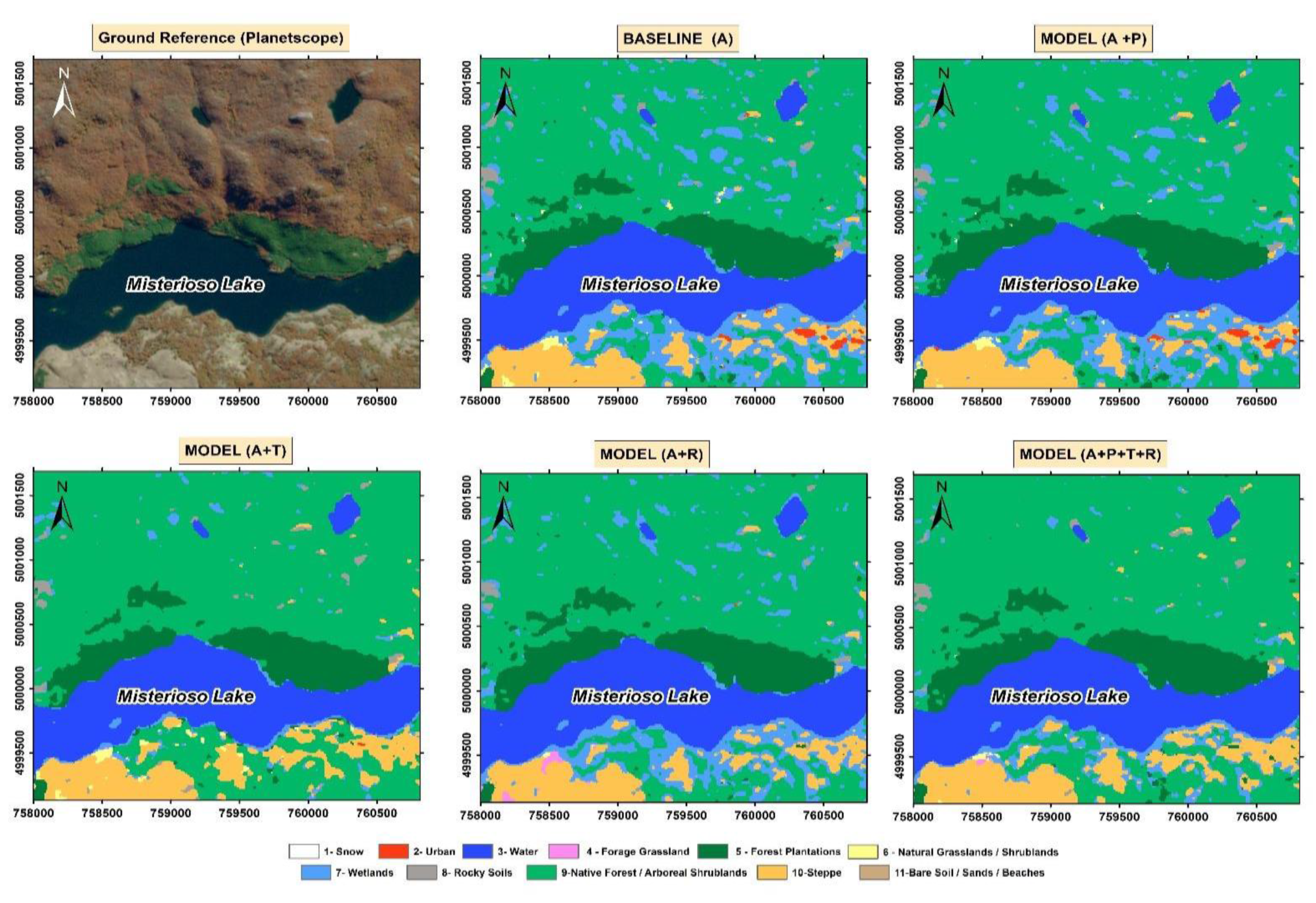
Table 3.
Definition of land use and land cover classes.
| Class | General description | |
|---|---|---|
| 1 | Snow | Surfaces of persistent snow or ice (glaciers/ice fields). |
| 2 | Urban | Built-up areas, road infrastructure, and artificial surfaces. |
| 3 | Water | Inland water bodies (lakes, rivers, reservoirs). |
| 4 | Forage grassland | Managed herbaceous vegetation for livestock production (rotational pastures). |
| 5 | Forest plantation | Exotic fast-growing monocultures (pine, eucalyptus, or other species). |
| 6 | Natural grasslands / shrublands | Transitional natural shrub and herbaceous vegetation. |
| 7 | Wetlands | Areas saturated or flooded part of the year (wet meadows, peatlands, marshes, swamps) with hydrophilic vegetation. |
| 8 | Rocky terrain | Slopes, outcrops, and rocky massifs with sparse or absent vegetation; high reflectance and rough texture. |
| 9 | Native / mixed forest | Forest formations dominated by native species with dense canopy cover. |
| 10 | Steppe | Discontinuous xerophytic vegetation (coirón grass) associated with semi-arid conditions. |
| 11 | Bare soil / sands / alluvial beaches | Sediments, sand flats, fluvial beaches, and eroded areas lacking vegetation cover. |
Table 4.
Summary of global performance metrics (Overall Accuracy, Kappa coefficient, Balanced Accuracy, and Macro-F1) obtained for the five evaluated classification model configurations (A, A+P, A+T, A+R, and Full).
Table 4.
Summary of global performance metrics (Overall Accuracy, Kappa coefficient, Balanced Accuracy, and Macro-F1) obtained for the five evaluated classification model configurations (A, A+P, A+T, A+R, and Full).
| Model | OA (%) | κ | BA (%) | Macro-F1 (%) |
|---|---|---|---|---|
| A (optical) | 89.2 | 0.871 | 86.1 | 80.5 |
| A+P (optical+P) | 89.6 (+0.4) | 0.876 (+0.005) | 86.9 (+0.8) | 81.7 (+1.2) |
| A+T (optical+T) | 90.3 (+1.1) | 0.883 (+0.012) | 87.4 (+1.3) | 84.3 (+3.8) |
| A+R (optical+R) | 91.7 (+2.5) | 0.899 (+0.028) | 88.4 (+2.3) | 84.3 (+3.8) |
| Full (A+P+T+R) | 92.5 (+3.3) | 0.905 (+0.034) | 89.0 (+2.9) | 86.0 (+5.5) |
Disclaimer/Publisher’s Note: The statements, opinions and data contained in all publications are solely those of the individual author(s) and contributor(s) and not of MDPI and/or the editor(s). MDPI and/or the editor(s) disclaim responsibility for any injury to people or property resulting from any ideas, methods, instructions or products referred to in the content. |
© 2026 by the authors. Licensee MDPI, Basel, Switzerland. This article is an open access article distributed under the terms and conditions of the Creative Commons Attribution (CC BY) license (http://creativecommons.org/licenses/by/4.0/).
Copyright: This open access article is published under a Creative Commons CC BY 4.0 license, which permit the free download, distribution, and reuse, provided that the author and preprint are cited in any reuse.


