Electromagnetic Induction Back-Action as a Passive Mechanical Memory Kernel: From Lumped RL Maxwell Elements to Conducting Half-Space Diffusion (and Flux-Quantized Superconducting Rings)

1. Introduction

1.1. The Point: Induction Back-Action Is Generically a Passive Memory Kernel

A moving permanent magnet near a conductor induces currents. Those currents act back on the magnet. This is commonly reduced to one of two idealizations:

1.

Conservative approximation: an added stiffness derived from magnetostatic energy;

2.

Viscous approximation: an added damping coefficient proportional to velocity (eddy-current braking).

• Both approximations are correct only in restricted limits. The more universal phenomenological fact is:

• Induction back-action is causal and history dependent. Finite inductive storage and diffusion imply that the induced current pattern cannot respond instantaneously to motion. Therefore the force is not a function of the instantaneous state alone but is a convolutional functional of motion history. Because the underlying electrodynamics is passive (resistors dissipate; inductors store), the resulting mechanical kernel is passive as well.

1.2. Why This Is Often “Overlooked” in Practice

The kernel is not conceptually exotic—it is enforced by Maxwell–Faraday and passivity—but it is often operationally overlooked because:

1.

The limiting laws (stiffness-only or damping-only) are convenient and often numerically adequate in narrow bands.

2.

In many engineering contexts one measures only an effective k and c at a single frequency, which hides the phase-lag structure.

3.

Distributed conductors (plates, housings, cryostats) produce broad relaxation spectra; a single $(R,L)$ fit misses the continuum and can mis-predict phase and scaling.

This paper aims to make the kernel explicit in a way that is (i) energy-consistent (passive), (ii) geometry-calibrated, and (iii) extensible from lumped loops to diffusion continua.

1.3. Model Ladder and Contributions

We develop the idea through three levels:

Level 0: general passive two-port.

A coupling coefficient G and an electrical impedance $Z\left(s\right)$ determine a mechanical kernel via

$$K_{\mathrm{em}}\left(s\right)={\displaystyle \frac{G^{2}s}{Z\left(s\right)}}.$$

This is the most compact statement of “electromagnetic back-action as a network-synthesizable mechanical memory kernel.”

Level 1: dipole–lumped loop (single pole).

For $Z\left(s\right)=R+sL$ one obtains the exact Maxwell element kernel $K_{\mathrm{em}}\left(\omega \right)=G^{2}i\omega /(R+i\omega L)$, including a passivity/energy identity and parameter identification.

Level 2: dipole above a conducting half-space (diffusion).

A real plate is not a single RL mode. We derive an explicit spectral (Hankel-transform) kernel for a dipole oscillating normal to a conducting half-space. The result is a passive diffusion branch-cut kernel controlled by $\mathrm{\Omega }=s\mu \sigma h^2$ and with correct viscous and image-spring asymptotes.

Optional: superconducting ring (fluxoid quantization).

Flux quantization yields piecewise-conservative force laws and flux jumps that create discrete-state memory (hysteresis).

2. General Electromechanical Kernel from Impedance (Passive Two-Port)

2.1. Small-Signal Kinematics and the Induced Emf

We use a scalar mechanical coordinate $x\left(t\right)$ (e.g., axial position). Linearize around a bias point $x_0$:

$$x\left(t\right)=x_0+\xi \left(t\right),\left|\xi \right|\ll (\mathrm{geometric}\mathrm{scale}).$$

Let $\mathrm{\Lambda }\left(x\right)$ denote flux linkage between the moving magnet and a chosen electrical generalized coordinate (a loop current, a modal eddy-current coordinate, etc.).

Define the coupling gradient

$$G:={\mathrm{\Lambda }}^{\prime }\left(x_0\right).$$

(1)

To first order,

$$\mathrm{\Lambda }\left(x\left(t\right)\right)\approx \mathrm{\Lambda }\left(x_0\right)+G\xi \left(t\right).$$

(2)

Maxwell–Faraday implies the induced emf

$$e\left(t\right)=-\dot{\mathrm{\Lambda }}\left(t\right)\approx -G\dot{\xi }\left(t\right).$$

(3)

2.2. Co-Energy Transduction: Force Proportional to Current

For a linear electromechanical transducer in this one-degree coupling, magnetic co-energy gives

$$F_{\mathrm{em}}\left(t\right)=Gi\left(t\right),$$

(4)

where i is the electrical generalized current conjugate to $\mathrm{\Lambda }$.

2.3. Impedance Form: Kernel from $Z\left(s\right)$

Let the electrical environment seen by the induced emf be characterized (in Laplace domain) by a causal impedance $Z\left(s\right)$, so that

$$I\left(s\right)={\displaystyle \frac{E\left(s\right)}{Z\left(s\right)}}.$$

Using (3) and (4),

$$F_{\mathrm{em}}\left(s\right)=GI\left(s\right)=-{\displaystyle \frac{G^{2}s}{Z\left(s\right)}}\mathrm{\Xi }\left(s\right).$$

Define the (complex) dynamic stiffness

$$K_{\mathrm{em}}\left(s\right):=-{\displaystyle \frac{F_{\mathrm{em}}\left(s\right)}{\mathrm{\Xi }\left(s\right)}}={\displaystyle \frac{G^{2}s}{Z\left(s\right)}}.$$

(5)

2.4. Passivity Statement

If $Z\left(s\right)$ is positive real (PR), i.e., realizable by a passive electrical network, then the admittance $Y\left(s\right)=1/Z\left(s\right)$ is PR. Define the induced mechanical impedance (force/velocity)

$$Z_{\mathrm{mech}}\left(s\right):={\displaystyle \frac{F}{V}}={\displaystyle \frac{K_{\mathrm{em}}\left(s\right)}{s}}=G^{2}Y\left(s\right).$$

A nonnegative scalar multiple of a PR function is PR, hence $Z_{\mathrm{mech}}$ is PR: the induced mechanical element is passive.

This is the core structural constraint that the “stiffness-only” and “damping-only” approximations can violate if used outside their asymptotic regimes.

3. Baseline Example: Dipole–Lumped Loop (Single RL Pole)

This section is the cleanest case and fixes notation. It is also the local building block of generalized-Maxwell (multi-mode) fits.

3.1. Dipole–Loop Flux Linkage and Coupling Gradient

Consider a magnetic dipole moment $m=m\widehat{z}$ on the symmetry axis of a circular loop of radius a lying in the plane $z=0$. Let x be the dipole axial coordinate measured from the loop center.

Under the dipole approximation, the azimuthal vector potential is

$$A_{\phi }(\rho ,z)={\displaystyle \frac{{\mu }_{0}m\rho }{4\pi {({\rho }^2+z^2)}^{3/2}}}.$$

(6)

The flux through one turn is

$$\mathrm{\Phi }\left(x\right)=\oint A·dl=2\pi a{A}_{\phi }(a,x)={\displaystyle \frac{{\mu }_{0}m{a}^2}{2{(a^2+x^2)}^{3/2}}}.$$

(7)

Differentiating,

$${\mathrm{\Phi }}^{\prime }\left(x\right)=-{\displaystyle \frac{3{\mu }_{0}m{a}^{2}x}{2{(a^2+x^2)}^{5/2}}}.$$

(8)

For an N-turn loop, $\mathrm{\Lambda }\left(x\right)=N\mathrm{\Phi }\left(x\right)$ and

$$G={\mathrm{\Lambda }}^{\prime }\left(x_0\right)=N{\mathrm{\Phi }}^{\prime }\left(x_0\right).$$

(9)

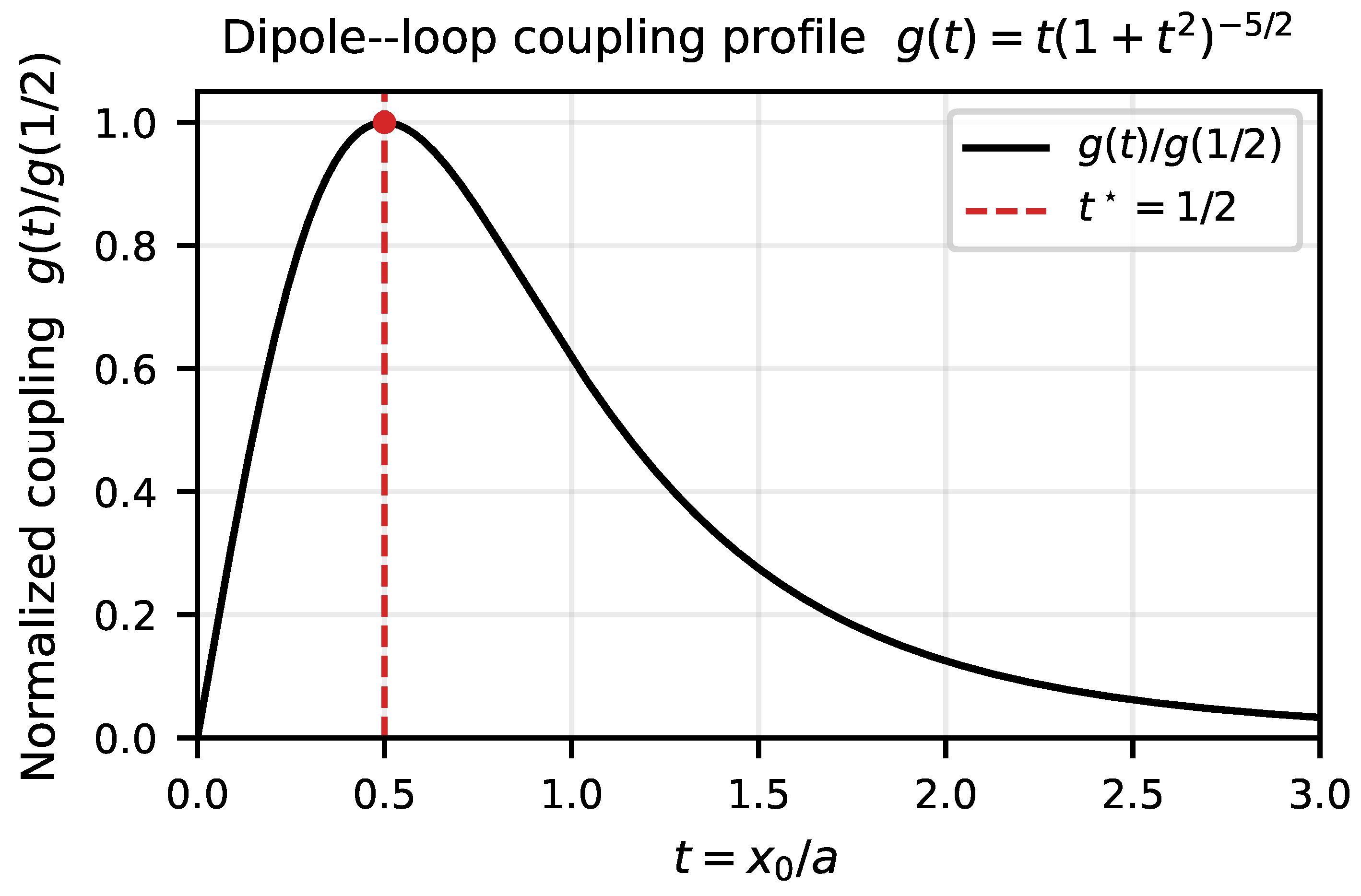
3.2. Design Rule (Dipole–Loop): Maximal Coupling at $x_0=a/2$

From (8), $\left|G\right|\propto |x_0|/{(a^2+x_0^2)}^{5/2}$. Setting $t=x_0/a$, maximizing $t/{(1+t^2)}^{5/2}$ yields a maximum at $t^{★}=1/2$:

$$x_0^{★}={\displaystyle \frac{a}{2}}.$$

(10)

Figure 1. (From your original draft.) Normalized dipole–loop coupling profile proportional to $\left|G\right|$, maximized at $x_0/a=1/2$.

Figure 1. (From your original draft.) Normalized dipole–loop coupling profile proportional to $\left|G\right|$, maximized at $x_0/a=1/2$.

3.3. Circuit + Force Law and Maxwell-Element Kernel

For a lumped loop with resistance R and inductance L, the total linkage is

$$\lambda \left(t\right)=Li\left(t\right)+\mathrm{\Lambda }\left(x\right(t\left)\right).$$

Faraday + Ohm give

$$L\dot{i}+Ri=-{\mathrm{\Lambda }}^{\prime }\left(x\right)\dot{x}.$$

(11)

Linearizing about $x_0$ gives

$$L\dot{i}+Ri=-G\dot{\xi },F_{\mathrm{em}}=Gi.$$

(12)

Eliminating i yields an internal-state force law:

$${\dot{F}}_{\mathrm{em}}+{\displaystyle \frac{1}{\tau }}{F}_{\mathrm{em}}=-k_{\infty }\dot{\xi },\tau \equiv {\displaystyle \frac{L}{R}},k_{\infty }\equiv {\displaystyle \frac{G^2}{L}}.$$

(13)

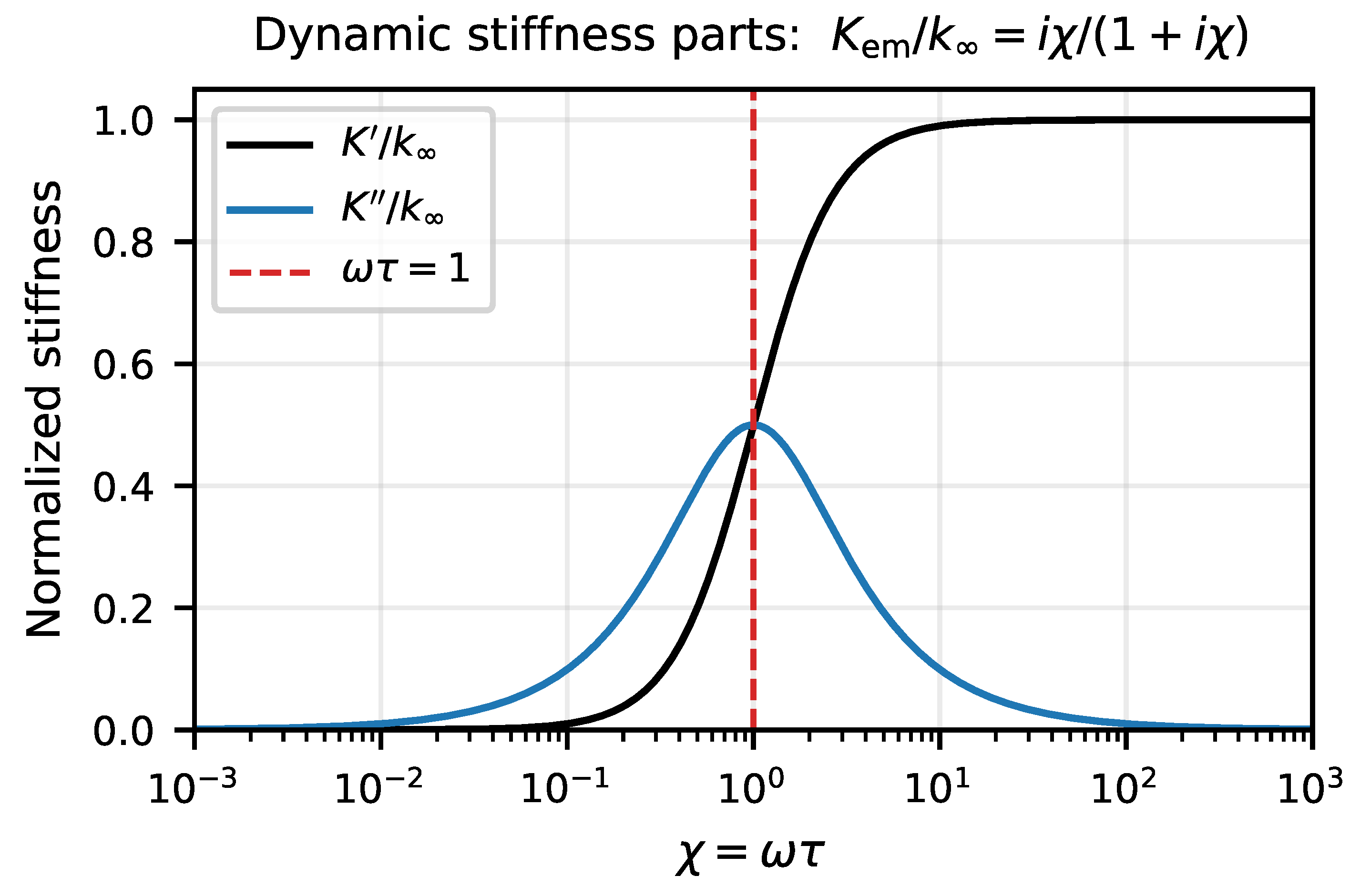
Under harmonic motion $\xi \left(t\right)=\Re \left[X{e}^{i\omega t}\right]$, the dynamic stiffness is

$$K_{\mathrm{em}}\left(\omega \right)={\displaystyle \frac{G^{2}i\omega }{R+i\omega L}}=k_{\infty }{\displaystyle \frac{i\omega \tau }{1+i\omega \tau }}.$$

(14)

This is exactly the dynamic stiffness of a mechanical Maxwell element (spring $k_{\infty }$ in series with dashpot $c_0=k_{\infty }\tau =G^2/R$).

3.4. Passivity/Energy Identity (Lumped RL)

Embed the coupling in a mechanical resonator

$$M\ddot{\xi }+c_m\dot{\xi }+k_m\xi =F_{\mathrm{em}}+F_{\mathrm{drv}}.$$

Define stored energy

$$E\left(t\right)=\frac{1}{2}M{\dot{\xi }}^2+\frac{1}{2}{k}_m{\xi }^2+\frac{1}{2}L{i}^2.$$

Multiplying the mechanical equation by $\dot{\xi }$ and the circuit equation by i yields

$$\dot{E}\left(t\right)=-c_m{\dot{\xi }}^2-R{i}^2+\dot{\xi }{F}_{\mathrm{drv}}\left(t\right),$$

(15)

so for $F_{\mathrm{drv}}=0$, $c_m\ge 0$, $R\ge 0$, the coupled system is passive.

3.5. Identification from Complex Stiffness (Single Pole)

If $K_{\mathrm{em}}\left(\omega \right)=K^{\prime }\left(\omega \right)+i{K}^{\prime \prime }\left(\omega \right)$ is measured and follows (14), then

$$\omega \tau ={\displaystyle \frac{K^{\prime }}{K^{\prime \prime }}}\Rightarrow \tau ={\displaystyle \frac{1}{\omega }}{\displaystyle \frac{K^{\prime }}{K^{\prime \prime }}},$$

(16)

and

$$k_{\infty }={\displaystyle \frac{{\left(K^{\prime }\right)}^2+{\left(K^{\prime \prime }\right)}^2}{K^{\prime }}}.$$

(17)

These identities will be used later as a controlled approximation when fitting diffusion continua by an “effective Maxwell” kernel.

Figure 2. (From your original draft.) Normalized RL-loop dynamic stiffness decomposition.

Figure 2. (From your original draft.) Normalized RL-loop dynamic stiffness decomposition.

4. Where Single-Pole RL Breaks: Distributed Conductors

A real conductor (plate, shield, cryostat wall) does not behave as a single lumped loop with fixed $(R,L)$. Eddy currents are spatially distributed; the magnetic field diffuses into the conductor with diffusivity

$$D={\displaystyle \frac{1}{\mu \sigma }}.$$

This produces:

• a broad relaxation spectrum (multi-mode / continuum),
• a branch-cut frequency response (square-root structure), and
• geometry-controlled crossovers governed by h (distance) and the diffusion time $\mu \sigma h^2$.

The next section (Part 2 of this draft) derives the exact passive kernel for the canonical geometry: a vertical magnetic dipole oscillating normal to a conducting half-space.

5. Dipole Above a Conducting Half-Space: Exact Diffusion Kernel

5.1. Geometry, Assumptions, and What Is Being Computed

Consider a nonmagnetic conducting half-space occupying $z<0$ with conductivity $\sigma$ and permeability $\mu$ (typically $\mu \approx {\mu }_0$ for Cu/Al). The region $z>0$ is vacuum (or air) with permeability ${\mu }_0$ and negligible conductivity.

A point magnetic dipole of fixed moment

$$m=m\widehat{z}$$

is located on the symmetry axis at height

$$h\left(t\right)=h_0+\xi \left(t\right),\left|\xi \right|\ll h_0,$$

above the interface $z=0$. The mechanical coordinate is the height perturbation $\xi \left(t\right)$.

We seek the linearized electromagnetic back-action force

$$F_{\mathrm{em}}\left(t\right)\approx -\left(k_{\mathrm{add}}*\xi \right)\left(t\right)$$

and, equivalently, the Laplace/frequency-domain dynamic stiffness

$$K_{\mathrm{em}}\left(s\right):=-{\displaystyle \frac{F_{\mathrm{em}}\left(s\right)}{\mathrm{\Xi }\left(s\right)}}.$$

Quasi-static validity.

We use the magnetoquasistatic approximation: displacement current is negligible in Ampère’s law, while Faraday induction is retained. A standard sufficient condition in the conductor is $\omega ϵ/\sigma \ll 1$ and length scales small relative to $c/\omega$.

Because the source and geometry are axisymmetric and the dipole is normal to the surface, the fields may be represented by an azimuthal vector potential

$$A(\rho ,z,t)=A_{\phi }(\rho ,z,t)\widehat{\phi }.$$

Then $B=\nabla \times A$ has components

$$B_{\rho }=-{\displaystyle \frac{\partial A_{\phi }}{\partial z}},B_z={\displaystyle \frac{1}{\rho }}{\displaystyle \frac{\partial }{\partial \rho }}\left(\rho A_{\phi }\right).$$

(18)

In the vacuum region ($z>0$), there are no conduction currents, and in Coulomb gauge one has Laplace’s equation for the scattered field:

$$\left({\nabla }^2-{\rho }^{-2}\right)A_{\phi }=0(z>0,\mathrm{away}\mathrm{from}\mathrm{the}\mathrm{dipole}\mathrm{source}).$$

(19)

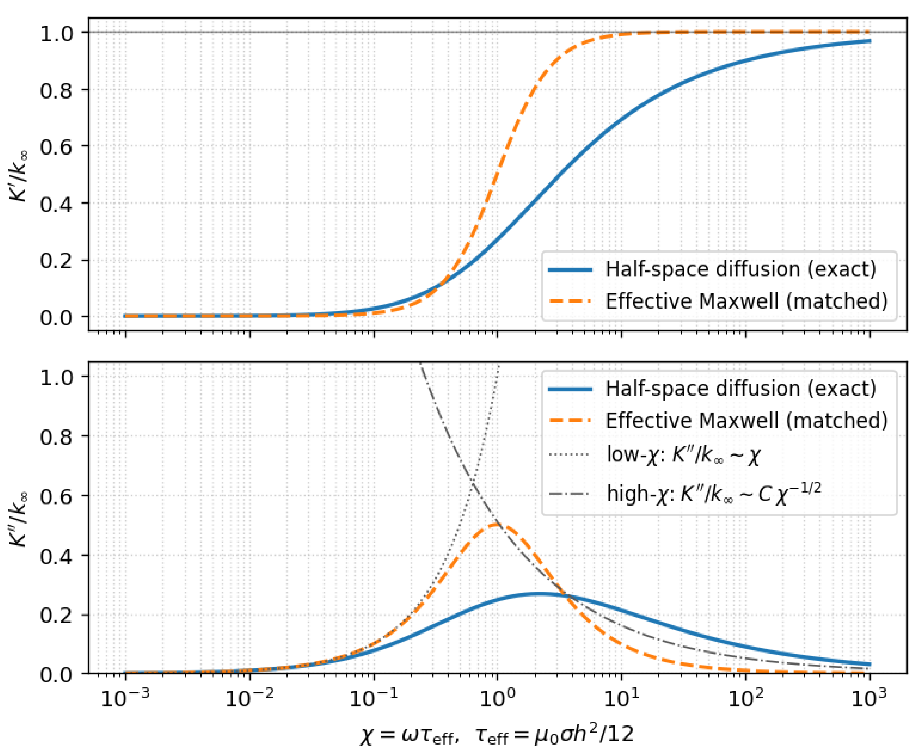
Figure 3. Normalized complex stiffness for a vertical dipole above a conducting half-space. Solid: exact diffusion kernel from (42) evaluated at $\mathrm{\Omega }=ı12\chi$. Dashed: effective Maxwell fit with ${\tau }_{\mathrm{eff}}={\mu }_0\sigma h^2/12$. The diffusion kernel exhibits a ${\chi }^{-1/2}$ high-frequency loss tail, unlike the $1/\chi$ decay of a single pole.

Figure 3. Normalized complex stiffness for a vertical dipole above a conducting half-space. Solid: exact diffusion kernel from (42) evaluated at $\mathrm{\Omega }=ı12\chi$. Dashed: effective Maxwell fit with ${\tau }_{\mathrm{eff}}={\mu }_0\sigma h^2/12$. The diffusion kernel exhibits a ${\chi }^{-1/2}$ high-frequency loss tail, unlike the $1/\chi$ decay of a single pole.

In the conductor ($z<0$), Ohm’s law and Faraday’s law give an eddy current density

$$J=\sigma E\approx -\sigma {\displaystyle \frac{\partial A}{\partial t}},$$

and Ampère’s law (without displacement current) yields the diffusion equation

$$\left({\nabla }^2-{\rho }^{-2}\right)A_{\phi }=\mu \sigma {\displaystyle \frac{\partial A_{\phi }}{\partial t}}(z<0).$$

(20)

In Laplace domain (with variable s),

$$\left({\nabla }^2-{\rho }^{-2}\right)A_{\phi }(\rho ,z;s)=\mu \sigma s{A}_{\phi }(\rho ,z;s)(z<0).$$

(21)

5.2. Hankel (Sommerfeld) spectral representation

We use the order-1 Hankel transform pair (cylindrical symmetry):

$$A_{\phi }(\rho ,z;s)={\int }_0^{\infty }\tilde{A}(k,z;s)J_1\left(k\rho \right)kdk.$$

(22)

Substituting (22) into (19)–(21) reduces the PDEs to ODEs in z for each spectral wavenumber k.

Vacuum ($z>0$).

Each mode satisfies

$${\displaystyle \frac{{\partial }^2\tilde{A}}{\partial z^2}}-k^2\tilde{A}=0,z>0,$$

(23)

so scattered components decay as $e^{-kz}$.

Conductor ($z<0$).

Each mode satisfies

$${\displaystyle \frac{{\partial }^2\tilde{A}}{\partial z^2}}-q^2(k,s)\tilde{A}=0,q(k,s):=\sqrt{k^2+\mu \sigma s},z<0,$$

(24)

and the physical solution is $\tilde{A}\propto e^{qz}$, which decays as $z\to -\infty$. We choose the principal square root branch with Re $q(k,s)>0$ for Re $s>0$.

5.3. Incident Dipole Field in HANKEL Form

For a vertical point dipole at height h in free space, the azimuthal vector potential is

$$A_{\phi }^{\mathrm{dip}}(\rho ,z;h)={\displaystyle \frac{{\mu }_{0}m\rho }{4\pi {\left({\rho }^2+{(z-h)}^2\right)}^{3/2}}}.$$

Using the standard identity

$${\displaystyle \frac{\rho }{{\left({\rho }^2+a^2\right)}^{3/2}}}={\int }_0^{\infty }{J}_1\left(k\rho \right)k{e}^{-k\left|a\right|}dk,$$

we obtain the Hankel representation

$$A_{\phi }^{\mathrm{dip}}(\rho ,z;h)={\displaystyle \frac{{\mu }_{0}m}{4\pi }}{\int }_0^{\infty }{e}^{-k|z-h|}{J}_1\left(k\rho \right)kdk.$$

(25)

Therefore, the incident spectral amplitude is simply

$${\tilde{A}}_{\mathrm{inc}}(k,z;h)={\displaystyle \frac{{\mu }_{0}m}{4\pi }}{e}^{-k|z-h|}.$$

(26)

In particular, the incident amplitude at the interface $z=0^{+}$ is

$${\tilde{A}}_{\mathrm{inc}}(k,0^{+};h)={\displaystyle \frac{{\mu }_{0}m}{4\pi }}{e}^{-kh}.$$

(27)

5.4. Interface Matching and the Diffusion Reflection Coefficient

Write the total vacuum-side field as incident plus reflected:

$${\tilde{A}}_{+}(k,z;s)={\tilde{A}}_{\mathrm{inc}}(k,z;h_0)+{\tilde{A}}_{\mathrm{ref}}(k,z;s),z>0,$$

and the conductor field as

$${\tilde{A}}_{-}(k,z;s)={\tilde{A}}_{\mathrm{cond}}(k,z;s),z<0.$$

At $z=0$ we impose the standard magnetoquasistatic boundary conditions: continuity of $A_{\phi }$ and continuity of tangential H (equivalently $(1/\mu ){\partial }_z{A}_{\phi }$ for this polarization). This yields, for each k,

$${\tilde{A}}_{+}(k,0^{+};s)={\tilde{A}}_{-}(k,0^{-};s),{\displaystyle \frac{1}{{\mu }_0}}{\displaystyle \frac{\partial {\tilde{A}}_{+}}{\partial z}}(k,0^{+};s)={\displaystyle \frac{1}{\mu }}{\displaystyle \frac{\partial {\tilde{A}}_{-}}{\partial z}}(k,0^{-};s).$$

(28)

Because ${\tilde{A}}_{\mathrm{ref}}(k,z;s)\propto e^{-kz}$ and ${\tilde{A}}_{\mathrm{cond}}(k,z;s)\propto e^{qz}$, one obtains the standard diffusion reflection coefficient

$$r(k,s)={\displaystyle \frac{{\displaystyle \frac{k}{{\mu }_0}-\frac{q(k,s)}{\mu }}}{{\displaystyle \frac{k}{{\mu }_0}+\frac{q(k,s)}{\mu }}}}={\displaystyle \frac{\mu k-{\mu }_{0}q(k,s)}{\mu k+{\mu }_{0}q(k,s)}}.$$

(29)

For the common nonmagnetic case $\mu ={\mu }_0$, this simplifies to

$$r(k,s)={\displaystyle \frac{k-q(k,s)}{k+q(k,s)}},q(k,s)=\sqrt{k^2+{\mu }_0\sigma s}.$$

(30)

As expected:

$$r(k,0)=0\left(\mathrm{no}\mathrm{DC}\mathrm{eddy}\mathrm{currents}\right),r(k,s)\to -1\mathrm{as}\left|s\right|\to \infty (\mathrm{AC}\mathrm{exclusion}/\mathrm{skin}\mathrm{effect}).$$

5.5. Linearization with Respect to Vertical Motion

The only time dependence is through the height $h\left(t\right)=h_0+\xi \left(t\right)$. From (27), the incident boundary amplitude is

$${\tilde{A}}_{\mathrm{inc}}(k,0^{+};t)={\displaystyle \frac{{\mu }_{0}m}{4\pi }}{e}^{-k(h_0+\xi \left(t\right))}\approx {\displaystyle \frac{{\mu }_{0}m}{4\pi }}{e}^{-k{h}_0}\left(1-k\xi \left(t\right)\right).$$

The constant term ($\propto 1$) produces no reflected field because $r(k,0)=0$. Thus the dynamic boundary drive is

$$\delta {\tilde{A}}_{\mathrm{inc}}(k,0^{+};s)=-{\displaystyle \frac{{\mu }_{0}m}{4\pi }}k{e}^{-k{h}_0}\mathrm{\Xi }\left(s\right).$$

(31)

The reflected spectral field in vacuum is then

$$\delta {\tilde{A}}_{\mathrm{ref}}(k,z;s)=r(k,s)\delta {\tilde{A}}_{\mathrm{inc}}(k,0^{+};s)e^{-kz}=-{\displaystyle \frac{{\mu }_{0}m}{4\pi }}kr(k,s)e^{-k(h_0+z)}\mathrm{\Xi }\left(s\right).$$

(32)

Evaluated at the dipole location $z=h_0$,

$$\delta {\tilde{A}}_{\mathrm{ref}}(k,h_0;s)=-{\displaystyle \frac{{\mu }_{0}m}{4\pi }}kr(k,s)e^{-2k{h}_0}\mathrm{\Xi }\left(s\right).$$

(33)

5.6. Force on the Dipole and the Exact Dynamic Stiffness Integral

We compute the induced $B_z$ on the axis using (18). From (22), one finds (using $(1/\rho ){\partial }_{\rho }\left(\rho J_1\left(k\rho \right)\right)=k{J}_0\left(k\rho \right)$)

$$B_z(\rho ,z;s)={\int }_0^{\infty }\tilde{A}(k,z;s)k^2{J}_0\left(k\rho \right)dk.$$

(34)

On the axis $\rho =0$ (where $J_0\left(0\right)=1$),

$$B_z(0,z;s)={\int }_0^{\infty }\tilde{A}(k,z;s)k^{2}dk.$$

(35)

Using (32), the reflected (induced) axial field at the dipole is

$$\delta B_z^{\mathrm{ref}}(0,h_0;s)={\int }_0^{\infty }\delta {\tilde{A}}_{\mathrm{ref}}(k,h_0;s)k^{2}dk=-{\displaystyle \frac{{\mu }_{0}m}{4\pi }}\mathrm{\Xi }\left(s\right){\int }_0^{\infty }r(k,s)k^3{e}^{-2k{h}_0}dk.$$

(36)

For a dipole with fixed moment $m=m\widehat{z}$ in an external field, the force is

$$F_z={\displaystyle \frac{\partial }{\partial z}}\left(m{B}_z\right)=m{\displaystyle \frac{\partial B_z}{\partial z}}.$$

Differentiate (36) with respect to the observation coordinate z (equivalently, use ${\partial }_z{e}^{-k(h_0+z)}=-k{e}^{-k(h_0+z)}$ in (32)):

$$F_{\mathrm{em}}\left(s\right)=m{\left.{\displaystyle \frac{\partial }{\partial z}}\delta B_z^{\mathrm{ref}}(0,z;s)\right|}_{z=h_0}={\displaystyle \frac{{\mu }_0{m}^2}{4\pi }}\mathrm{\Xi }\left(s\right){\int }_0^{\infty }r(k,s)k^4{e}^{-2k{h}_0}dk.$$

(37)

Therefore the exact small-signal dynamic stiffness is

$$K_{\mathrm{em}}\left(s\right):=-{\displaystyle \frac{F_{\mathrm{em}}\left(s\right)}{\mathrm{\Xi }\left(s\right)}}=-{\displaystyle \frac{{\mu }_0{m}^2}{4\pi }}{\int }_0^{\infty }r(k,s)k^4{e}^{-2k{h}_0}dk.$$

(38)

Using (30) (nonmagnetic conductor, $\mu ={\mu }_0$) and writing $-r=(q-k)/(q+k)$, we obtain the explicit diffusion form

$$K_{\mathrm{em}}\left(s\right)={\displaystyle \frac{{\mu }_0{m}^2}{4\pi }}{\int }_0^{\infty }{k}^4{e}^{-2k{h}_0}{\displaystyle \frac{q(k,s)-k}{q(k,s)+k}}dk,q(k,s)=\sqrt{k^2+{\mu }_0\sigma s}.$$

(39)

Structural point.

Equation (39) is not rational in s because $q=\sqrt{k^2+{\mu }_0\sigma s}$. The half-space is therefore not representable by any finite number of RL poles; it is a diffusion (branch-cut) kernel, equivalent to an infinite RL ladder / continuous relaxation spectrum.

5.7. Nondimensionalization: The Single Governing Diffusion Parameter

Let $p=k{h}_0$ and define the dimensionless diffusion frequency

$$\mathrm{\Omega }:={\mu }_0\sigma s{h}_0^2.$$

(40)

Then (39) becomes

$$K_{\mathrm{em}}\left(s\right)={\displaystyle \frac{{\mu }_0{m}^2}{4\pi h_0^5}}\mathcal{K}\left(\mathrm{\Omega }\right),$$

(41)

with the dimensionless kernel

$$\mathcal{K}\left(\mathrm{\Omega }\right)={\int }_0^{\infty }{p}^4{e}^{-2p}{\displaystyle \frac{\sqrt{p^2+\mathrm{\Omega }}-p}{\sqrt{p^2+\mathrm{\Omega }}+p}}dp.$$

(42)

Thus the entire frequency dependence is governed by $\mathrm{\Omega }=s\left({\mu }_0\sigma h_0^2\right)$, i.e. the diffusion time scale

$${\tau }_D\sim {\mu }_0\sigma h_0^2.$$

5.8. Asymptotic Limits and the “Effective Maxwell” Time Constant

Although (42) is a diffusion kernel (branch cut), its low- and high-frequency limits reduce to the familiar damping-only and stiffness-only laws.

5.8.1. Low Frequency: Viscous Limit (Dashpot)

For $\left|\mathrm{\Omega }\right|\ll 1$, one has $\sqrt{p^2+\mathrm{\Omega }}=p+\mathrm{\Omega }/\left(2p\right)+O({\mathrm{\Omega }}^2/p^3)$ for fixed $p>0$, hence

$${\displaystyle \frac{\sqrt{p^2+\mathrm{\Omega }}-p}{\sqrt{p^2+\mathrm{\Omega }}+p}}={\displaystyle \frac{\mathrm{\Omega }/\left(2p\right)+\dots }{2p+\dots }}={\displaystyle \frac{\mathrm{\Omega }}{4p^2}}+O\left({\mathrm{\Omega }}^2\right).$$

Substitute into (42):

$$\mathcal{K}\left(\mathrm{\Omega }\right)={\displaystyle \frac{\mathrm{\Omega }}{4}}{\int }_0^{\infty }{p}^2{e}^{-2p}dp+O\left({\mathrm{\Omega }}^2\right)={\displaystyle \frac{\mathrm{\Omega }}{4}}·{\displaystyle \frac{1}{4}}+O\left({\mathrm{\Omega }}^2\right)={\displaystyle \frac{\mathrm{\Omega }}{16}}+O\left({\mathrm{\Omega }}^2\right),$$

(43)

since ${\int }_0^{\infty }{p}^2{e}^{-2p}dp=2!/2^3=1/4$. Therefore,

$$K_{\mathrm{em}}\left(s\right)={\displaystyle \frac{{\mu }_0{m}^2}{4\pi h_0^5}}\left({\displaystyle \frac{\mathrm{\Omega }}{16}}+O\left({\mathrm{\Omega }}^2\right)\right)=c_{0}s+O\left(s^2\right),$$

(44)

with viscous coefficient

$$c_0={\displaystyle \frac{{\mu }_0{m}^2}{4\pi h_0^5}}·{\displaystyle \frac{{\mu }_0\sigma h_0^2}{16}}={\displaystyle \frac{{\mu }_0^2\sigma m^2}{64\pi h_0^3}}.$$

(45)

Thus for slow motion ($\omega {\tau }_D\ll 1$),

$$F_{\mathrm{em}}\left(t\right)\approx -c_0\dot{\xi }\left(t\right).$$

5.8.2. High Frequency: Image-Spring Limit (Elastic Stiffness)

For $\left|\mathrm{\Omega }\right|\gg 1$, $\sqrt{p^2+\mathrm{\Omega }}=\sqrt{\mathrm{\Omega }}\sqrt{1+p^2/\mathrm{\Omega }}$ and the ratio tends to 1 for each fixed p:

$${\displaystyle \frac{\sqrt{p^2+\mathrm{\Omega }}-p}{\sqrt{p^2+\mathrm{\Omega }}+p}}\to 1.$$

Hence

$$\mathcal{K}\left(\mathrm{\Omega }\right)\to {\int }_0^{\infty }{p}^4{e}^{-2p}dp={\displaystyle \frac{4!}{2^5}}={\displaystyle \frac{24}{32}}={\displaystyle \frac{3}{4}}.$$

(46)

Therefore the high-frequency stiffness is

$$k_{\infty }:=\underset{\left|s\right|\to \infty }{lim}{K}_{\mathrm{em}}\left(s\right)={\displaystyle \frac{{\mu }_0{m}^2}{4\pi h_0^5}}·{\displaystyle \frac{3}{4}}={\displaystyle \frac{3{\mu }_0{m}^2}{16\pi h_0^5}}.$$

(47)

This is the “image-spring” limit: the conductor excludes the AC component of the field, generating an approximately conservative restoring force about the bias height.

5.8.3. High-Frequency Diffusion Correction: Fractional $s^{-1/2}$ Tail

The diffusion nature appears strongly in the approach to $k_{\infty }$. For large $\left|\mathrm{\Omega }\right|$, expand

$${\displaystyle \frac{\sqrt{p^2+\mathrm{\Omega }}-p}{\sqrt{p^2+\mathrm{\Omega }}+p}}=1-{\displaystyle \frac{2p}{\sqrt{p^2+\mathrm{\Omega }}+p}}\sim 1-{\displaystyle \frac{2p}{\sqrt{\mathrm{\Omega }}}}+O\left({\mathrm{\Omega }}^{-1}\right).$$

Substituting into (42) gives

$$\mathcal{K}\left(\mathrm{\Omega }\right)={\displaystyle \frac{3}{4}}-{\displaystyle \frac{2}{\sqrt{\mathrm{\Omega }}}}{\int }_0^{\infty }{p}^5{e}^{-2p}dp+O\left({\mathrm{\Omega }}^{-1}\right)={\displaystyle \frac{3}{4}}-{\displaystyle \frac{2}{\sqrt{\mathrm{\Omega }}}}·{\displaystyle \frac{5!}{2^6}}+O\left({\mathrm{\Omega }}^{-1}\right)={\displaystyle \frac{3}{4}}-{\displaystyle \frac{15}{8}}{\mathrm{\Omega }}^{-1/2}+O\left({\mathrm{\Omega }}^{-1}\right).$$

(48)

Thus

$$K_{\mathrm{em}}\left(s\right)=k_{\infty }-{\displaystyle \frac{{\mu }_0{m}^2}{4\pi h_0^5}}·{\displaystyle \frac{15}{8}}{\mathrm{\Omega }}^{-1/2}+O\left({\mathrm{\Omega }}^{-1}\right).$$

(49)

Because ${\mathrm{\Omega }}^{-1/2}\propto s^{-1/2}$, this is a fractional diffusion tail (a branch-cut signature). For harmonic $s=i\omega$,

$${\left(i\omega \right)}^{-1/2}={\omega }^{-1/2}{e}^{-i\pi /4},$$

so $K^{\prime }\left(\omega \right)$ approaches $k_{\infty }$ from below while $K^{\prime \prime }\left(\omega \right)$ decays as ${\omega }^{-1/2}$ with a fixed ${45}^{\circ }$ phase contribution.

5.8.4. A Controlled Single-Pole Approximation (Effective Maxwell Element)

Even though the half-space kernel is not single-pole, one can define an effective Maxwell element by matching the two asymptotes:

$$K_{\mathrm{Maxwell}}\left(s\right)=k_{\infty }{\displaystyle \frac{s{\tau }_{\mathrm{eff}}}{1+s{\tau }_{\mathrm{eff}}}},K_{\mathrm{Maxwell}}\left(s\right)\sim \left(k_{\infty }{\tau }_{\mathrm{eff}}\right)s\mathrm{as}s\to 0.$$

Matching the low-frequency dashpot coefficient $c_0$ in (45) gives

$${\tau }_{\mathrm{eff}}:={\displaystyle \frac{c_0}{k_{\infty }}}={\displaystyle \frac{{\displaystyle \frac{{\mu }_0^2\sigma m^2}{64\pi h_0^3}}}{{\displaystyle \frac{3{\mu }_0{m}^2}{16\pi h_0^5}}}}={\displaystyle \frac{{\mu }_0\sigma h_0^2}{12}}.$$

(50)

5.8.4.1. Interpretation.

${\tau }_{\mathrm{eff}}$ is (up to the factor $1/12$) the magnetic diffusion time across the geometric distance $h_0$. It provides a useful order-of-magnitude crossover frequency,

$${\omega }_{\mathrm{c}}\sim {\tau }_{\mathrm{eff}}^{-1}\sim {\displaystyle \frac{12}{{\mu }_0\sigma h_0^2}},$$

but it does not imply that the half-space is truly single-relaxation-time; the exact kernel has a continuous spectrum (Part 3).

5.9. Summary of the Half-Space Result

For a vertical dipole oscillating normally above a conducting half-space, the exact small-signal electromagnetic back-action stiffness is the diffusion integral

$$K_{\mathrm{em}}\left(s\right)={\displaystyle \frac{{\mu }_0{m}^2}{4\pi }}{\int }_0^{\infty }{k}^4{e}^{-2k{h}_0}{\displaystyle \frac{\sqrt{k^2+{\mu }_0\sigma s}-k}{\sqrt{k^2+{\mu }_0\sigma s}+k}}dk.$$

It is passive, causal, and controlled by the single dimensionless parameter $\mathrm{\Omega }={\mu }_0\sigma s{h}_0^2$. Its limits recover:

$$K_{\mathrm{em}}\left(s\right)\sim c_{0}s\left(\right|\mathrm{\Omega }|\ll 1),K_{\mathrm{em}}\left(s\right)\to k_{\infty }\left(\right|\mathrm{\Omega }|\gg 1),$$

with

$$c_0={\displaystyle \frac{{\mu }_0^2\sigma m^2}{64\pi h_0^3}},k_{\infty }={\displaystyle \frac{3{\mu }_0{m}^2}{16\pi h_0^5}},{\tau }_{\mathrm{eff}}={\displaystyle \frac{{\mu }_0\sigma h_0^2}{12}}.$$

6. Diffusion Kernel as a Continuous Relaxation Spectrum (Generalized Maxwell / RL Ladder)

6.1. Why Diffusion Implies a Continuum of Relaxation Times

The conductor half-space is governed (in the conductor) by the diffusion equation

$${\partial }_t{A}_{\phi }=D({\nabla }^2-{\rho }^{-2})A_{\phi },D={\displaystyle \frac{1}{\mu \sigma }}.$$

After Hankel transform in $\rho$, each lateral wavenumber k contributes a depth diffusion operator with eigenvalue $k^2$. Thus even before enforcing the boundary coupling to the dipole, the half-space already contains a continuum of characteristic rates

$${\lambda }_k\sim D{k}^2={\displaystyle \frac{k^2}{\mu \sigma }}.$$

This is the physical origin of the non-rational square-root dependence $q(k,s)=\sqrt{k^2+\mu \sigma s}$ and the branch-cut structure of the exact stiffness integral (39).

In network language: diffusion is equivalent to an infinite RL ladder (a distributed impedance), not a finite $(R,L)$.

6.2. A Key Scalar Identity: Square-Root Reflection as a Mixture of Debye Relaxations

For the nonmagnetic case $\mu ={\mu }_0$, the half-space stiffness (39) involves the scalar factor

$${\displaystyle \frac{\sqrt{k^2+\alpha s}-k}{\sqrt{k^2+\alpha s}+k}},\alpha :={\mu }_0\sigma .$$

Write

$$\sqrt{k^2+\alpha s}=k\sqrt{1+u},u:={\displaystyle \frac{\alpha s}{k^2}},$$

and define

$$f\left(u\right):={\displaystyle \frac{\sqrt{1+u}-1}{\sqrt{1+u}+1}}.$$

(51)

Then the reflection factor is exactly $f(\alpha s/k^2)$.

The following representation makes the continuous Maxwell spectrum explicit.

Proposition (continuous Debye/Maxwell mixture).

For Re $u>0$,

$$f\left(u\right)={\int }_1^{\infty }{\displaystyle \frac{u}{u+t}}\rho \left(t\right)dt,\rho \left(t\right)={\displaystyle \frac{2}{\pi }}{\displaystyle \frac{\sqrt{t-1}}{t^2}}.$$

(52)

Moreover, $\rho \left(t\right)\ge 0$ and ${\int }_1^{\infty }\rho \left(t\right)dt=1$.

Interpretation.

Each factor ${\displaystyle \frac{u}{u+t}}$ is a single-pole Debye relaxation in u. Thus $f\left(u\right)$ is a continuum of single-pole relaxations with a positive density $\rho \left(t\right)$ supported on $t\ge 1$. This is exactly the structure of a generalized Maxwell (Prony-series) element in the continuum limit.

Sketch of verification.

The identity (52) can be checked by evaluating both sides on the imaginary axis and using the Stieltjes inversion formula for the representation

$$f\left(u\right)={\int }_0^{\infty }{\displaystyle \frac{u}{u+t}}\nu \left(dt\right)\Rightarrow {\nu }^{\prime }\left(t\right)={\displaystyle \frac{1}{\pi t}}Imf(-t+i0).$$

For (51), the branch cut starts at $u\le -1$, so $\nu$ is supported on $t\ge 1$ and yields the stated density.

6.3. Continuous-Maxwell Form of the Half-Space Stiffness

Insert (52) into the exact stiffness integral (39). Using $u=\alpha s/k^2$,

$$f\left({\displaystyle \frac{\alpha s}{k^2}}\right)={\int }_1^{\infty }{\displaystyle \frac{s}{s+\frac{k^2}{\alpha }t}}\rho \left(t\right)dt.$$

Therefore the half-space stiffness can be written as the two-layer continuum

$$K_{\mathrm{em}}\left(s\right)={\displaystyle \frac{{\mu }_0{m}^2}{4\pi }}{\int }_0^{\infty }{k}^4{e}^{-2k{h}_0}\left({\int }_1^{\infty }{\displaystyle \frac{s}{s+\frac{k^2}{\alpha }t}}\rho \left(t\right)dt\right)dk,\alpha ={\mu }_0\sigma .$$

(53)

Network/viscoelastic analogy.

Equation (53) is a generalized Maxwell representation:

$$K_{\mathrm{em}}\left(s\right)=\int {\displaystyle \frac{s}{s+\lambda }}d\nu \left(\lambda \right),$$

with a positive measure $\nu$ induced by the geometry weight $k^4{e}^{-2k{h}_0}$ and the diffusion density $\rho \left(t\right)$. Any finite RL-ladder / finite generalized-Maxwell approximation corresponds to quadrature of the $(k,t)$ continuum.

6.4. Why a Finite Derivative Expansion Fails (Nonanalyticity and Memory Tails)

In Sec. 5 we found the low-frequency expansion

$$K_{\mathrm{em}}\left(s\right)=c_{0}s-c_1{s}^2+\dots ,c_0={\displaystyle \frac{{\mu }_0^2\sigma m^2}{64\pi h_0^3}},c_1={\displaystyle \frac{{\mu }_0^3{\sigma }^2{m}^2}{64\pi h_0}}.$$

Attempting to extend this to $O\left(s^3\right)$ produces a divergent coefficient: the integral that would generate the $s^3$ term is not integrable near $k\to 0$. This is the analytic fingerprint of diffusion: the true function has a branch cut and therefore contains noninteger powers (and/or logarithmic terms) in its asymptotics.

Equivalently: diffusion produces long memory (broad relaxation spectrum), so no finite-order local differential operator can represent it outside a narrow band.

7. Practical Evaluation, Fitting, and Identification

7.1. Fast Numerical Evaluation of the Exact Kernel

The scaled form (41)–(42) is convenient:

$$K_{\mathrm{em}}\left(s\right)={\displaystyle \frac{{\mu }_0{m}^2}{4\pi h_0^5}}\mathcal{K}\left(\mathrm{\Omega }\right),\mathrm{\Omega }={\mu }_0\sigma s{h}_0^2,$$

$$\mathcal{K}\left(\mathrm{\Omega }\right)={\int }_0^{\infty }{p}^4{e}^{-2p}{\displaystyle \frac{\sqrt{p^2+\mathrm{\Omega }}-p}{\sqrt{p^2+\mathrm{\Omega }}+p}}dp.$$

Because of the $e^{-2p}$ factor, one may truncate at $p_{max}\approx 10$–15 for high accuracy. For harmonic response $s=i\omega$, use the principal square root for $\sqrt{p^2+i\omega {\mu }_0\sigma h_0^2}$.

7.2. Two-Parameter Similarity Form and Collapse

The half-space model has a strict two-parameter similarity structure:

$$K_{\mathrm{em}}\left(i\omega \right)=A\mathcal{K}\left(i\omega T\right),A:={\displaystyle \frac{{\mu }_0{m}^2}{4\pi h_0^5}},T:={\mu }_0\sigma h_0^2.$$

(54)

Thus all frequency responses collapse onto a universal curve $\mathcal{K}\left(ix\right)$ after rescaling frequency by T and stiffness by A.

7.3. Asymptote-Based Extraction of $(m,\sigma )$ When Frequency Range Is Broad

If measurements reach the asymptotic regimes:

1.

at high frequency, $K^{\prime }\left(\omega \right)\to k_{\infty }$ with

$$k_{\infty }={\displaystyle \frac{3{\mu }_0{m}^2}{16\pi h_0^5}},$$

2.

at low frequency, $K\left(i\omega \right)\sim i\omega c_0$ so $c_{\mathrm{add}}\left(\omega \right)=K^{\prime \prime }\left(\omega \right)/\omega \to c_0$ with

$$c_0={\displaystyle \frac{{\mu }_0^2\sigma m^2}{64\pi h_0^3}},$$

then:

$$m^2={\displaystyle \frac{16\pi h_0^5}{3{\mu }_0}}{k}_{\infty },\sigma ={\displaystyle \frac{64\pi h_0^3}{{\mu }_0^2{m}^2}}{c}_0.$$

(55)

Alternatively, the ratio yields the diffusion time scale (independent of m):

$${\tau }_{\mathrm{eff}}={\displaystyle \frac{c_0}{k_{\infty }}}={\displaystyle \frac{{\mu }_0\sigma h_0^2}{12}}.$$

(56)

7.4. Full-Curve Fitting When Asymptotes Are Not Accessible

If the measured band does not reach the viscous or elastic plateau, fit the full complex curve to the similarity form (54) by treating $(A,T)$ as free parameters. Then reconstruct:

$$m=\sqrt{{\displaystyle \frac{4\pi h_0^5}{{\mu }_0}}A},\sigma ={\displaystyle \frac{T}{{\mu }_0{h}_0^2}}.$$

This can be done by complex least squares on $K\left(i\omega \right)$, or by fitting separately to $K^{\prime }\left(\omega \right)$ and $K^{\prime \prime }\left(\omega \right)$ with shared parameters.

7.5. Finite-Mode Generalized-Maxwell Approximation (Passive Rational Fit)

If a reduced-order model is required (e.g., for time-domain simulation in a mechanical controller), fit the diffusion kernel by a passive Prony series:

$$K_{\mathrm{em}}\left(s\right)\approx \sum _{n=1}^{N_m}{k}_n{\displaystyle \frac{s{\tau }_n}{1+s{\tau }_n}},k_n\ge 0,{\tau }_n>0.$$

(57)

This is a generalized Maxwell element (parallel sum of Maxwell branches). The representation (53) guarantees that such an approximation exists with nonnegative weights. A convenient practical choice is to fix ${\tau }_n$ logarithmically spaced around ${\tau }_{\mathrm{eff}}$ and solve for $k_n\ge 0$ by nonnegative least squares on complex frequency-response data.

Caution.

A single Maxwell element can match $c_0$ and $k_{\infty }$ via ${\tau }_{\mathrm{eff}}=c_0/k_{\infty }$, but it will not reproduce the square-root branch-cut phase behavior. Use (57) with multiple modes if phase accuracy matters.

8. Superconducting Rings: Fluxoid Quantization and Discrete-State Magnetomechanical Memory

This section is logically independent of the conducting half-space, but it illustrates the same “kernel/constraint” thesis: electromagnetic back-action is a constrained passive response, and in superconductors the constraint is topological (fluxoid quantization), producing a qualitatively different kind of memory.

8.1. Fluxoid Quantization Constraint

For a superconducting loop with inductance L magnetically coupled to a moving magnet with linkage $\mathrm{\Lambda }\left(x\right)$, fluxoid quantization imposes (in the simplest lumped description)

$$Li\left(t\right)+\mathrm{\Lambda }\left(x\right(t\left)\right)=n\mathrm{\Phi }0,n\in \mathbb{Z}.$$

(58)

Here $\mathrm{\Phi }0=h/\left(2e\right)\approx 2.07e-15$ Wb is the superconducting flux quantum.

Between phase slips, n is constant and (58) is algebraic:

$$i_n\left(x\right)={\displaystyle \frac{n\mathrm{\Phi }0-\mathrm{\Lambda }\left(x\right)}{L}}.$$

(59)

The electromagnetic force is still $F=i{\mathrm{\Lambda }}^{\prime }\left(x\right)$, hence

$$F_n\left(x\right)={\displaystyle \frac{(n\mathrm{\Phi }0-\mathrm{\Lambda }\left(x\right)){\mathrm{\Lambda }}^{\prime }\left(x\right)}{L}}.$$

(60)

This is conservative with potential energy

$$U_n\left(x\right)={\displaystyle \frac{{(n\mathrm{\Phi }0-\mathrm{\Lambda }\left(x\right))}^2}{2L}},F_n\left(x\right)=-d{U}_{n}x.$$

(61)

8.2. Small-Signal Stiffness in a Fixed Fluxoid Sector

Linearizing about a bias point $x_0$ in a fixed n gives

$$K_{\mathrm{sc}}\left(x_0\right):=-{\left.d{F}_{n}x\right|}_{x_0}={\displaystyle \frac{{\mathrm{\Lambda }}^{\prime }{\left(x_0\right)}^2}{L}}-{\displaystyle \frac{(n\mathrm{\Phi }0-\mathrm{\Lambda }\left(x_0\right)){\mathrm{\Lambda }}^{\prime \prime }\left(x_0\right)}{L}}.$$

(62)

If the trapped fluxoid n is such that $n\mathrm{\Phi }0\approx \mathrm{\Lambda }\left(x_0\right)$, then

$$K_{\mathrm{sc}}\left(x_0\right)\approx {\displaystyle \frac{{\mathrm{\Lambda }}^{\prime }{\left(x_0\right)}^2}{L}},$$

a purely elastic back-action (no dissipation), which may be viewed as the “$R\to 0$” limit of the lumped RL Maxwell element but with the crucial added constraint that the state is confined to discrete fluxoid sectors.

8.3. Phase Slips / Flux Jumps: Discrete-State Hysteresis and Force Steps

In real superconducting rings, n can change by $\pm 1$ via phase slips (vortex crossings) when the supercurrent approaches a critical value $I_c$ or when activation over a barrier occurs. A minimal hybrid-state model is:

• continuous state $i\left(t\right)$, discrete state $n\left(t\right)\in \mathbb{Z}$,
• between events: $Li+\mathrm{\Lambda }\left(x\right)=n\mathrm{\Phi }0$,
• event: $n\leftarrow n\pm 1$, which produces a current jump $\Delta i=\mp \mathrm{\Phi }0/L$.

The corresponding force jump (using $F=i{\mathrm{\Lambda }}^{\prime }\left(x\right)$) is

$$\Delta F={\mathrm{\Lambda }}^{\prime }\left(x\right)\Delta i=\mp {\displaystyle \frac{{\mathrm{\Lambda }}^{\prime }\left(x\right)\mathrm{\Phi }0}{L}}.$$

(63)

Thus the mechanical observability of a flux jump is controlled by $|{\mathrm{\Lambda }}^{\prime }\left(x\right)|$, exactly the same coupling-gradient quantity that controls the linear kernel strength in normal conductors. This connects directly to your dipole–loop design rule: choosing the bias point that maximizes $\left|G\right|$ also maximizes $\left|\Delta F\right|$.

If the thresholds for $n\mapsto n\pm 1$ differ depending on the direction of motion (metastability), the resulting F–x relation is hysteretic: a genuine electromagnetic memory not representable by any linear time-invariant kernel.

9. Discussion and Conclusions

9.1. What the “Passive Memory Kernel” Viewpoint Buys You

The central statement is not “a particular transfer function,” but a structural constraint:

Electromagnetic induction back-action is generically a passive, causal mechanical memory kernel whose form is dictated by the impedance/diffusion physics of the induced currents.

For a lumped loop, that kernel is a single Maxwell element. For a conducting half-space, the kernel is a diffusion branch-cut function with a continuum of relaxation times, which can be expressed explicitly as a continuous generalized-Maxwell spectrum. For superconducting rings, fluxoid quantization replaces linear dissipation by discrete-state conservative sectors punctuated by flux-jump events, producing nonlinear hysteretic memory.

9.2. Summary of Main Results

1.

A general small-signal electromechanical kernel formula:

$$K_{\mathrm{em}}\left(s\right)={\displaystyle \frac{G^{2}s}{Z\left(s\right)}},$$

which makes passivity and causality transparent when $Z\left(s\right)$ is passive.

2.

For a vertical dipole above a conducting half-space, an exact diffusion stiffness integral:

$$K_{\mathrm{em}}\left(s\right)={\displaystyle \frac{{\mu }_0{m}^2}{4\pi }}{\int }_0^{\infty }{k}^4{e}^{-2k{h}_0}{\displaystyle \frac{\sqrt{k^2+{\mu }_0\sigma s}-k}{\sqrt{k^2+{\mu }_0\sigma s}+k}}dk,$$

and its similarity reduction to a universal dimensionless function of $\mathrm{\Omega }={\mu }_0\sigma s{h}_0^2$.

3.

Closed-form asymptotes:

$$K\left(s\right)\sim c_{0}s,c_0={\displaystyle \frac{{\mu }_0^2\sigma m^2}{64\pi h_0^3}}(\omega {\tau }_D\ll 1),$$

$$K\left(s\right)\to k_{\infty },k_{\infty }={\displaystyle \frac{3{\mu }_0{m}^2}{16\pi h_0^5}}(\omega {\tau }_D\gg 1),$$

and the effective crossover time ${\tau }_{\mathrm{eff}}={\mu }_0\sigma h_0^2/12$.

4.

A continuous generalized-Maxwell representation of the square-root reflection factor, exhibiting a positive relaxation density and proving that diffusion corresponds to an infinite passive ladder.

5.

For superconducting rings, fluxoid quantization yields piecewise-conservative force laws and flux jumps with force step magnitude $\left|\Delta F\right|=|{\mathrm{\Lambda }}^{\prime }|{\mathrm{\Phi }}_0/L$.

9.3. Future Extensions

Natural next steps are: (i) finite-thickness plates and multilayers (which replace the half-space diffusion factor by a thickness-dependent coth/tanh factor and introduce additional crossovers), (ii) non-axisymmetric motion (lateral drag) and dipole orientations parallel to the surface, (iii) finite-size magnets (beyond point dipole), and (iv) experimental validation with complex stiffness measurement and parameter extraction.

References

- Jackson, J. D. Classical Electrodynamics, 3rd ed.; Wiley, 1998. [Google Scholar]
- Griffiths, D. J. Introduction to Electrodynamics, 4th ed.; Pearson, 2012. [Google Scholar]
- Stratton, J. A. Electromagnetic Theory; McGraw–Hill, 1941. [Google Scholar]
- Landau, L. D.; Lifshitz, E. M. Electrodynamics of Continuous Media, 2nd ed.; Pergamon, 1984. [Google Scholar]
- Reitz, J. R. Forces on moving magnets due to eddy currents. Journal of Applied Physics 1970, vol. 41, 2067–2071. [Google Scholar] [CrossRef]
- Saslow, W. M. Maxwell’s theory of eddy currents in a conducting cylinder. American Journal of Physics 1992, vol. 60(no. 8), 693–711. [Google Scholar] [CrossRef]
- Wait, J. R. Electromagnetic Waves in Stratified Media, 2nd ed.; Pergamon, 1970. [Google Scholar]
- Lakes, R. S. Viscoelastic Materials; Cambridge University Press, 2009. [Google Scholar]
- Tinkham, M. Introduction to Superconductivity, 2nd ed.; McGraw–Hill, 1996. [Google Scholar]
- Deaver, B. S.; Fairbank, W. M. Experimental evidence for quantized flux in superconducting cylinders. Physical Review Letters 1961, vol. 7, 43–46. [Google Scholar] [CrossRef]
- Doll, R.; Näbauer, M. Experimental proof of magnetic flux quantization in a superconducting ring. Physical Review Letters 1961, vol. 7, 51–52. [Google Scholar] [CrossRef]
- Likharev, K. K. Dynamics of Josephson Junctions and Circuits; Gordon and Breach, 1986. [Google Scholar]
Disclaimer/Publisher’s Note: The statements, opinions and data contained in all publications are solely those of the individual author(s) and contributor(s) and not of MDPI and/or the editor(s). MDPI and/or the editor(s) disclaim responsibility for any injury to people or property resulting from any ideas, methods, instructions or products referred to in the content. |
© 2026 by the authors. Licensee MDPI, Basel, Switzerland. This article is an open access article distributed under the terms and conditions of the Creative Commons Attribution (CC BY) license (http://creativecommons.org/licenses/by/4.0/).
Copyright: This open access article is published under a Creative Commons CC BY 4.0 license, which permit the free download, distribution, and reuse, provided that the author and preprint are cited in any reuse.